The role of galaxies and AGN in reionising the IGM - II: metal-tracing the faint sources of reionisation at $5\lesssim z\lesssim 6$

Abstract

We present a new method to study the contribution of faint sources to the UV background using the 1D correlation of metal absorbers with the intergalactic medium (IGM) transmission in a Quasi Stellar Object (QSO) sightline. We take advantage of a sample of $25$ high signal-to-noise ratio QSO spectra to retrieve $150$ triply-ionised carbon (C IV) absorbers at $4.5\lesssim z\lesssim 6.2$, of which $37$ systems whose expected H I absorption lie in the Lyman-$\alpha$ forest. We derive improved constraints on the cosmic density of C IV at $4.3<z<6.2$ and infer from abundance-matching that C IV absorbers trace $M_{\text{UV}}\lesssim-16$ galaxies. Correlation with the Lyman-$\alpha$ forest of the QSOs indicates that these objects are surrounded by a highly opaque region at $r\lesssim 5$ cMpc/h followed by an excess of transmission at $r\gtrsim 10$ cMpc/h detected at $2.7\sigma$. This is in contrast to equivalent measurements at lower redshifts where only the opaque trough is detected. We interpret this excess as a statistical enhancement of the local photoionisation rate due to clustered faint galaxies around the C IV absorbers. Using the analytical framework described in Paper I of this series, we derive a constraint on the average product of the escape fraction and the Lyman continuum photon production efficiency of the galaxy population clustered around the C IV absorbers, $\log\langle f_{\text{esc}}\xi_{\text{ion}}\rangle/[{\rm erg^{-1}~{}Hz}]=25.01^{+0.30}_{-0.19}$. This implies that faint galaxies beyond the reach of current facilities may have harder radiation fields and/or larger escape fractions than currently detected objects at the end of the reionisation epoch.

1 Introduction

Cosmic reionisation has been the object of much scrutiny in the last decades, resulting in remarkable progress on the determination of its timing. The period during which most of the cosmic neutral hydrogen gas was reionised is now constrained to lie in the redshift interval $6\lesssim z\lesssim 15$ (Planck Collaboration et al., 2016). Evidence suggests that during this time it is actively star-forming galaxies that produced most of the required ionising photons (e.g. Robertson et al., 2013; Puchwein et al., 2018), although some debate currently exists around a possible contribution of active galactic nuclei (AGN) at $z\sim 6$ (Giallongo et al., 2015; D’Aloisio et al., 2017; Chardin et al., 2017; Parsa et al., 2018).

The major challenge in investigating the physical processes governing cosmic reionisation is the difficulty of probing the nature of the ionising radiation from sources at $z>7$. Deep surveys with the Hubble Space Telescope combined with the magnification of gravitational lensing by large clusters have recently pushed the census of galaxies to $z\sim 10$ (e.g. Bouwens et al., 2007; Ellis et al., 2013; Bouwens et al., 2015; Atek et al., 2015; Ishigaki et al., 2015; McLeod et al., 2015; Livermore et al., 2017; Ishigaki et al., 2018; Atek et al., 2018). However, at redshifts beyond $z\gtrsim 7$, only a handful of galaxies and active galactic nuclei have been spectroscopically confirmed and studied in any detail (e.g. Mortlock et al., 2011; Laporte et al., 2015; Roberts-Borsani et al., 2016; Laporte et al., 2017a, b; Bañados et al., 2018). A major impasse in understanding the role of star-forming galaxies is the uncertain fraction of ionising photons that can escape into the intergalactic medium (IGM). Using the demographics of galaxies observed out to redshifts $z\simeq$10 and the likely spectral energy distributions of young, metal-poor stellar populations, Robertson et al. (2015) estimate an average escape fraction of $f_{\text{esc}}\simeq$10-20% is required. Direct measures of the escape fraction are only possible at redshifts below $z\simeq$3 because Lyman continuum (LyC) photons emitted from star-forming galaxies are increasingly absorbed by the IGM at higher redshift.

In the meantime, the number and quality of quasi-stellar object (QSO) sightlines probing the IGM at the end of the reionisation era has multiplied quickly following systematic searches in the Sloan Digital Sky Survey (SDSS, Jiang et al., 2016), Panoramic Survey Telescope and Rapid Response System data(Pan-STARSS, Kaiser et al., 2010; Bañados et al., 2016), Dark Energy Survey - Visible and Infrared Survey Telescope for Astronomy (VISTA) Hemisphere Survey (DES-VHS, Reed et al., 2015), Subaru High-$z$ Exploration of Low-Luminosity Quasars survey (SHELLQS, Matsuoka et al., 2016) VISTA Kilo-Degree Infrared Galaxy Survey (VIKING, Venemans et al., 2013; Carnall et al., 2015) and UKIRT Infrared Deep Sky Survey (UKIDSS, Venemans et al., 2007; Mortlock et al., 2009, 2011). QSO sightlines offer a powerful tool to study the IGM at the end of the reionisation era (e.g. Fan et al., 2006; Becker et al., 2015) and the cosmic metal enrichment history (e.g. Ryan-Weber et al., 2009; Becker et al., 2009; D’Odorico et al., 2010, 2013). As a result of the increased number of sightlines now available (Bosman et al., 2018), a large scatter in the IGM opacity at $z\sim 6$ has been revealed with individual cases showing unexpected large opaque regions (Becker et al., 2015, 2018). The physical origin of these features remains unclear, although a late reionization model powered by galaxies claims to address these (Kulkarni et al., 2018).

In Kakiichi et al. (2018) (thereafter Paper I), we proposed a new method to directly measure the escape fraction of faint galaxies based on their clustering around luminous spectroscopically-confirmed galaxies which provide a local enhancement of transmission in the Lyman-$\alpha$ forest. By charting the distribution of galaxies close to the sightline of a bright QSO we constructed the cross-correlation with the IGM transmission, revealing a tentative indication of a statistical ‘proximity effect’. In the present study, we aim at measuring a similar correlation of galaxies to the IGM transmission but using a different tracer. Triply-ionised carbon (C IV) is the most common metal absorbing species in QSO spectra (Becker et al., 2009; D’Odorico et al., 2013, , thereafter DO13) and, at low redshifts, associated with the metal-enriched halos of galaxies (e.g. Adelberger et al., 2003, 2005; Steidel et al., 2010; Ford et al., 2013; Turner et al., 2014). At higher-redshift, little is known about the appropriate host galaxies, although some estimate these objects to have quite faint ultraviolet (UV) luminosities (Becker et al., 2015). It is however expected that C IV  absorbers lie $\lesssim 100$ pkpc from their host (e.g. Oppenheimer et al., 2009; Bird et al., 2016; Keating et al., 2016). More recently, (D’Odorico et al., 2018) reported the recent detection of a galaxy $40$ pkpc away from a DLA at $z\simeq 5.94$. Although there is no evidence for a consistent link between DLAs and C IV  absorbers at that redshift, the authors also report the potential detection of a weak associated C IV  absorption. This would support the idea that potential host galaxies can be found indeed very close to C IV  absorbers. Metal-tracing these faint sources should, in principle, allow us to probe the ionising capability of intrinsically faint galaxies well beyond reach of current spectroscopic facilities. Moreover, because metal absorbers lie directly on the QSO sightline, we can probe the IGM transmission around their hosts on the scales of $0.1\lesssim r\lesssim 1$ pMpc unattainable in the approach introduced in Paper I which uses nearby LBGs.

In this second paper in the series, we take advantage of a large sample of $z>5.4$ QSO spectra to study the abundance and distribution of C IV absorbers. We then study the 1D correlation of these absorbers with the IGM transmission measured in the Lyman-$\alpha$ forest of the QSO to assess their impact on the IGM. Our study focuses on C IV absorbers at $4.3<z<6.2$, but future possibilities include other metals and potentially studies of the redshift evolution of such correlations.

The plan for this paper is as follows. Section 2.1 introduces our observational sample of QSO spectra and the initial data reduction. Section 2.3 details our semi-automated search for C IV absorbers and the result of our search. We present in section 3 the new constraints on the $4.3<z<6.2$ C IV cosmic density derived from our large sample. We also present our measurement of the C IV-IGM transmission 1D correlation. Section 4 presents two models of the said correlation. In Section 5 we then discuss the nature of the C IV  absorbers host galaxies, and our evidence for an enhanced transmission in the IGM surrounding C IV absorbers. We put a constraint on the product of the escape fraction and the LyC photon production efficiency. We conclude in Section 6 with a brief summary of our findings and future prospects for this new method measuring the escape fraction at the end of the reionisation era.

Throughout this paper we adopt the Planck 2015 cosmology $(\Omega_{m},\Omega_{\Lambda},\Omega_{b},h,\sigma_{8},n_{s})=(0.3089,0.6911,0.04860,0.6774,0.8159,0.9667)$ (Planck Collaboration et al., 2016). We use pkpc and pMpc (ckpc and cMpc) to indicate distances in proper (comoving) units.

2 Methods

2.1 Observations

Table 1: QSO sightlines used in this work. References: (1) McGreer et al. (2015); (2) Bosman et al. (2018); (3) Becker et al. (2015); (4) Becker et al. (2006); (5) Eilers et al. (2017); (6) reduced from online archives in this work (see Table 2).

QSO name	$z$	Instrument	SNR	ref.
J1148+0702	6.419	HIRES	29.7	(1)
J0100+2802	6.30	XShooter	85.2	(2)
J1030+0524	6.28	XShooter	28.0	(1)
J0050+3445	6.25	ESI	24.4	(3)
J1048+4637	6.198	HIRES	29.2	(4)
J1319+0950	6.132	XShooter	96.8	(3)
J1509–1749	6.12	XShooter	88.9	(1)
J2315–0023	6.117	ESI	29.8	(3)
J1602+4228	6.09	ESI	33.3	(2)
J0353+0104	6.072	ESI	80.7	(3)
J0842+1218	6.07	ESI	18.0	(6)
J2054–0005	6.062	ESI	39.5	(3)
J1306+0356	6.016	XShooter	55.8	(1)
J1137+3549	6.01	ESI	31.7	(2)
J0818+1722	6.00	XShooter	114.0	(6)
J1411+1217	5.927	ESI	15.9	(1)
J0148+0600	5.923	XShooter	128.0	(3)
J0005–0006	5.85	ESI	28.8	(5)
J0840+5624	5.844	ESI	17.6	(1)
J0836+0054	5.81	XShooter	93.4	(1)
J0002+2550	5.80	ESI	121.0	(6)
J1044–0125	5.782	ESI	49.2	(3)
J0927+2001	5.772	XShooter	73.7	(3)
J1022+2252	5.47	ESI	19.0	(6)
J0231–0728	5.42	XShooter	115.0	(6)

Table 2: QSO sightlines in addition to those listed in Bosman et al. (2018). These spectra were reduced either from Keck Observatory Archive (KOA) data for the ESI spectrograph, or from the XShooter archive.

QSO name	$z$	Instrument	$t_{\text{total}}(s)$	SNR	ref.	PID	P.I.
J0842+1218	6.07	ESI	2400	18	De Rosa et al. (2011)	U085E	R. Becker
J0002+2550	5.80	ESI	22200	121	Fan et al. (2004)	H31aE	A. Cowie
						H46aE	Kakazu
J1022+2252	5.47	ESI	6000	19	–	U130Ei	G. Becker
J0818+1722	6.00	XShooter	20750	114	Fan et al. (2006),	084A-0550	D’Odorico
					D’Odorico et al. (2011)	086A-0574	De Rosa
						088A-0897	De Rosa
J0231–0728	5.42	XShooter	21600	115	Becker et al. (2012)	084A-0574	G. Becker

Our sample consists of $25$ optical spectra of quasars with $z_{\text{source}}>5.4$ originating from the Echellette Spectrograph and Imager (ESI) on the Keck II telescope (Sheinis et al., 2002), the XShooter instrument on Cassegrain UT2 (Vernet et al., 2011), and the High Resolution Echelle Spectrometer (HIRES, Vogt et al. 1994) as shown in Table 1. Out of these, 20 spectra are re-used from the quasar sample of Bosman et al. (2018). These spectra were selected for their high signal-to-noise ratios (SNR $>17$) measured over the $1265<\lambda<1275$ Å range via

$$\text{SNR}=\left<\frac{F}{\epsilon}\right>\cdot\sqrt{N_{60}}\,\text{,}$$ (1)

where $F$ is the flux, $\epsilon$ is the error, and $N_{60}$ is the number of spectral bins covering $60$ km s^-1 . An exception is the quasar J1411+1217 which is included despite its relatively poor SNR ($=15.9$) due to the presence of a particularly broad C IV absorber. Out of these objects, 7 originate in a study from McGreer et al. (2015) (3 of which were independently re-reduced), 6 from Becker et al. (2015), one from Becker et al. (2006), one from Eilers et al. (2017) (re-reduced), and 5 from Bosman et al. (2018) (of which 2 are archival).

Together with these $20$ sightlines, we reduced 5 additional spectra from the Keck Observatory Archive and the XShooter search tool for the ESO Science Archive Facility as summarised in Table 2. The spectra were extracted optimally making use of the calibration files (flat fields and standard star exposures) available in the archives for each set of observations. After performing sky subtraction, different observations of the same sightline are combined when necessary. The implementations of optimal extraction, sky subtraction, and telluric correction used herein are outlined in more detail in Horne (1986), Kelson (2003) and Becker et al. (2012) respectively. Our final sample contains ESI spectra with either $55.9$ km/s or $74.6$ km/s resolution depending on the slit, while XShooter spectra have either a $28.0$ km/s or $34.1$ km/s resolution and HIRES spectra have $6$ km/s resolution. We have re-binned the HIRES spectra by a factor $5$ to match the XShooter resolution to facilitate the search for C IV  absorbers redwards of Lyman-$\alpha$.

To measure transmitted Lyman-$\alpha$ fluxes bluewards of the Lyman-$\alpha$ emission line, we fit each spectrum with a power-law continuum. This power-law is fitted over the relatively featureless wavelength interval $1270$ Å–$1450$ Å in the rest frame. We exclude pixels affected by sky lines and use two rounds of sigma-clipping with thresholds of $|F_{\text{PL}}-F_{\text{obs}}|<2\epsilon$ and $1.5\epsilon$, where $\epsilon$ is the observational error and $F_{\text{PL}},F_{\text{obs}}$ are the values of the power-law fit and the quasar flux, respectively.

The Lyman-$\alpha$ forest of $z\gtrsim 5$ is characterised by high absorption at all wavelengths, making the continuum notoriously difficult to determine or model. Due to the sparsity of transmitted flux, we make no attempt at modelling the continuum bluewards of the Lyman-$\alpha$ emission line beyond a power-law. At lower redshift, more advanced techniques have been used and include subtracting profiles of weak intrinsic absorption and emission lines (e.g. Crighton et al. 2011). When comparing to such studies, a potential worry is a bias in the Lyman-$\alpha$ forest self-correlation on the scales of such features that are not removed by a simple power-law. We however verified that the self-correlation was not deviated from unity by more than 1$\sigma$ on any scale (see Bosman et al., 2018).

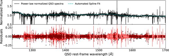
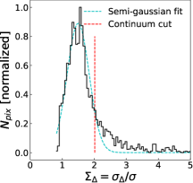
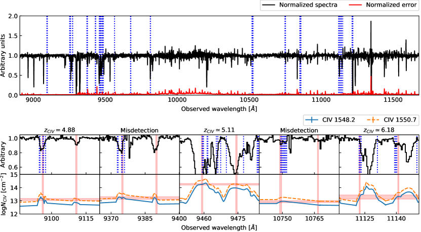
Figure 1: Illustration of our automated search procedure for C IV  absorbers as demonstrated for the QSO J0100+2802. Upper left panel: Measured (power-law normalized) flux in black, fitted continuum in cyan. The residuals present very little to no slow-varying residual trend and are consistent within the $2\sigma$ errors (red). Upper right panel: Histogram (black) of the $\Delta F$ variance $\sigma_{\Delta}$ divided by the “error array” variance $\sigma$, and the associated threshold (red line) for non-continuum pixels, taken to be a $1.5\sigma$ cut away from the mean of a Gaussian (cyan) fitted to the values lower than the expected mean of $\sqrt{2}$. Middle panel: The intrinsic continuum normalized flux (black) and noise (red) are overlaid with the algorithm-identified C IV  absorbers (indicated by blue dotted lines) (see Section 2.3 for the search strategy). Lower panel: Zoom-in on some flagged C IV  candidates from the middle panel. The algorithm computes the column density for both C IV  1548 Å, 1550 Å  at every pixel, and flags every pair with matching column density at the correct separation, with the tolerance indicated in red. False detections and misalignments due to sigma-clipping can be easily removed by eye or when fitting with vpfit.

2.2 QSO Broad Emission Lines and continuum fitting

Previous systematic searches for C IV or metal absorptions in the continuum of $z\simeq 6$ QSO (e.g. Ryan-Weber et al., 2009; Becker et al., 2011; Simcoe et al., 2011; D’Odorico et al., 2013; Bosman et al., 2017; Codoreanu et al., 2018) proceed by removing first the power-law continuum of the QSO and secondly fitting the Broad Emission Lines (BEL). The BEL fit is usually performed with splines in an iterative “by-eye” process where the user supervises the selection of knot points. Since our sample contains $25$ QSO spectra, we developed an automated QSO continuum spline fitting (redwards of Lyman-$\alpha$ only) further described below. The first step is to determine which part of the spectra are devoid of narrow emission lines or Broad Absorption Lines. A “fit-by-eye" procedure would select such regions as representative of the QSO continuum. In fact, human users select regions where the pixel-to-pixel flux variation is consistent with the error array. Mathematically, we expect that for a slowly varying spectrum with high enough resolution, the pixel-to-pixel flux difference is distributed as

$$\Delta F_{i}=F_{i}-F_{i+1}\sim\mathcal{N}(0,2\sigma_{i}^{2})\,\text{ , }$$ (2)

where $F_{i}$ is the flux recorded at pixel $i$, $\sigma_{i}$ the corresponding error, and $\mathcal{N}(\mu,\sigma^{2})$ the normal distribution with mean $\mu$ and variance $\sigma^{2}$. We thus estimate the variance of the flux difference $\sigma_{\Delta}$ by simply computing a running variance on the flux variation $\Delta F_{i}$. The running variance is taken as the square of the standard deviation of $\Delta F$ in a 40 pixel wide window centered on pixel $i$. We then take the ratio between the $\sigma_{\Delta}$ and the error array $\sigma$ at each pixel $i$. The distribution of the resulting variable, $\Sigma_{\Delta}=\sigma_{\Delta}/\sigma$ is a Gaussian distribution of mean $\sqrt{2}$ with a tail of larger values, as expected (see upper right corner of Fig. 1). We fit a Gaussian to the low-value wing of the distribution of $\Sigma_{\Delta}$ and exclude all pixels at $>N\sigma$ from the mean of the fitted Gaussian from the “continuum pixels”. $N$ is a parameter chosen by the user, and $1\leq N\leq 3$ is used for all our spectra. We note however that in large, completely absorbed features, the pixel-to-pixel variation differs from the noise distribution array only in the wings of the absorption. To remove pixels at the bottom of these absorption troughs, we run a matched-filter with a Gaussian kernel with a width of $5$ Å. Any pixel with $S/N_{\text{matched-filter}}$ greater than a chosen threshold (here $>3$) should be rejected from the continuum.

The second step of the algorithm is based on the idea that the BEL that provide the complexity of the QSO continuum fitting are not a nuisance but rather a powerful indicator of where the splines knot points should be located. Based on a BEL rest-frame wavelength list given by the user, we assign a knot point on top of each BEL with some tolerance (provided by the user as well, but $\sim 10$ Å is a reasonable choice), and another intermediate knot point in between each BEL knots. We minimize the $\chi^{2}$ of the spline fit on the previously selected continuum pixels by moving the knot points in the assigned tolerance regions to yield our final fit. An example of a resulting fit is shown in Fig. 1. The automated continuum method successfully fits the BEL features as well as avoiding the regions contaminated by skylines. The quicfit (QUasar Intrinsic Continuum FITter) code is publicly available at https://github.com/rameyer/QUICFit.

2.3 C IV  identification

It is possible to search for many metal absorber species redwards of the QSO Lyman-$\alpha$ emission at high-redshift, including amongst other O I, C II, Si II, N V, Si IV, Al II, Al III. However C IV  is the most useful due to its ubiquity and the fact that it is reliably identifiable as a doublet. Once the BEL and power-law continuum of the QSO are subtracted, the processed spectrum is searched for C IV  doublets. We use a semi-automated identification algorithm.

Following Bosman et al. (2017), we fit an inverted Gaussian profile to the optical depth $\tau=-\log F$ every $\Delta v\sim 10$ km s^-1 interval, and apply $3$ iterations of 2-$\sigma$ clipping to fit the most prominent feature only. We then estimate the column density for each C IV  transition following the apparent optical depth method (Savage & Sembach, 1991)

$$N_{\text{C{\tiny IV}}}=\frac{m_{e}c}{\pi e^{2}f\lambda}\int\ln G(v)\text{d}v\,\text{ , }$$ (3)

where $G(v)$ is the fitted inverted Gaussian profile, $f=0.095$ or $0.19$ is the oscillator strength for the $\lambda=1548.2,1550.8$ Å transitions, respectively.

We select all pairs of Gaussian absorption profiles with $\log N_{\text{C{\tiny IV}}}>12.5$ and with a discrepancy in redshift $\Delta z<R/c$, where $R$ is the resolution in km s^-1 and a discrepancy in column density $\Delta\log N_{\text{C{\tiny IV}}}$ within $2\sigma$ of the Gaussian fitting errors. We demonstrate in Fig. 1 the full fitting and search procedure on the sightline towards J0100+2802. The discrete nature of the search in wavelength space and the $\sigma$-clipping operations sometimes produces false detections or unreliable estimates of the column density of our absorbers. In order to account for these issues, these flagged candidates are then fitted with vpfit (Carswell & Webb, 2014) to confirm their nature and derive precise column densities.

To estimate the completeness of our search, we insert $1000$ mock C IV  absorbers for each of $b=10,20,30$ km s^-1 Doppler parameters and 0.2 dex increments in column density from $N_{\text{C{\tiny IV}}}=10^{12}$ to $10^{14}$ cm^-2. We achieve a $90$% completeness level around $\log N_{\text{C{\tiny IV}}}\simeq 14.0$ for all $3$ instruments, assuming a Doppler parameter of $b=30$ km s^-1 (see Fig. 2). This completeness is in good agreement with previous C IV  searches cited beforehand given the resolution and SNR of the QSO spectra at hand.

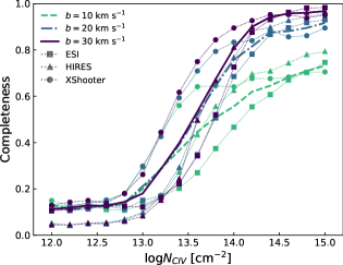
Figure 2: Completeness of our C IV  semi-automated retrieval computed by the insertion of $1000$ C IV  doublets at random redshifts in the ESI (squares), HIRES (triangles) and XShooter (dots) for different Doppler parameters $b=10,20,30$ km s^-1 (green, blue, purple). The thin lines represent the average values per instrument, whereas the bold lines represent the weighted average values for our sample.

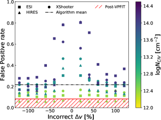
Figure 3: False positive rate of the algorithmic detection rate of C IV  candidates for various velocity displacements, instruments and column densities (coloured dots according to the right hand scale bar). The higher densities are more contaminated due to the tolerance on the optical fitting and the broad absorption wings of theses systems. The weighted mean false positive rate for our particular sample is indicated in dotted black, whereas the allowed values of the final false positive rate in our sample after visual inspection is shown in hatched red.

Table 3: Average completeness for the C IV  search. The completeness is a weighted average of the completeness values of Fig. 2 with $b=20$km/s for our specific set of QSO sightlines (HIRES:2, ESI:12, XShooter:13).

$\log N_{\text{C{\tiny IV}}}/[\text{cm}^{-2}]$	$13.0$	$13.2$	$13.4$	$13.6$	$13.8$	$14$
Completeness	$0.18$	$0.27$	$0.36$	$0.49$	$0.60$	$0.70$
$\log N_{\text{C{\tiny IV}}}/[\text{cm}^{-2}]$	$14.2$	$14.4$	$14.6$	$14.8$	$15.0$
Completeness	$0.78$	$0.82$	$0.84$	$0.85$	$0.87$

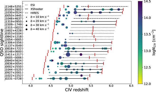
Figure 4: Redshift distribution of C IV  absorbers for $25$ QSO sightlines. The black lines show the full range of the Lyman-$\alpha$ forest for each QSO and the style of the line indicates the instrument. The red bars indicate the redshift range of our CIV search. The absorbers are shown as coloured dots whose size and colour coding reflect their Doppler $b$ parameter and column density, respectively.

An important issue is the possibility of false positives which would weaken the sought-after correlation. To assess the fraction of false positives in the candidates flagged by our algorithm, we first run the algorithm to search for doublet emission lines instead of absorption lines. This procedure should record no detections, but we sometimes recorded one or two detections per sightline due to glitches in the spectra or large residuals from continuum correction. Both kind of false positives were rejected when fitting with a Voigt profile with vpfit as they do not show the characteristic shape of genuine C IV  absorbers. We also insert mock absorbers with incorrect velocity spacing to assess the sensitivity of our algorithm to spuriously aligned absorption lines. We show in Fig. 3 the false positive rate for different velocity offsets of the two C IV  transitions from $25\%$ to $150\%$ relative error on the correct velocity spacing $\Delta v$ of the doublet. We find that the mean false positive rate is $\simeq 22\%$ for the algorithm search. We compute the mean false positive rate by weighting the false positive rates of each instrument by the number of QSO observed. Given that the candidates are inspected by eye while being fitted with vpfit, we expect the final false positive rate to be lower because some false positives are discarded. However, assessing the efficiency of a visual inspection is difficult. We compare our search with DO13 on $6$ matching sightlines where we found $56$ C IV  absorbers detections (see Section 2.4). Although we were more cautious than DO13 and rejected some of their absorbers, the fact that we found only two additional detections also argues against our technique generating false positives. Thus if the remainder of the $150$ C IV  sample is pure at the algorithm level ($<22\%$), then the false positive rate of our final sample is expected to be $\lesssim 8\%$.

Finally, our search results in $150$ C IV  absorber detections at $4.5<z<6.3$. Fig. 4 shows a graphical representation of the C IV  absorbers found. Appendix A presents a complete list of our detected C IV  absorbers.

2.4 Comparison with previous C IV  searches

We briefly compare our results for those QSO sightlines already searched for C IV  by previous authors to assess the purity of our method. All other detections on other sightlines are new detections and are listed in Table A as well as velocity plots in Appendix B for the reduced sample lying in the Lyman-$\alpha$ forest. Based on this comparison, we estimate our search to be in agreement, if somewhat more conservative, than previous C IV  searches. We note that small differences in the column densities (up to $\sim 0.2-0.3$) are easily explained by the continuum fitting differences. We also sometimes fit fewer components than previous searches. The excellent agreement in the total cosmic density of C IV  between previous studies and our measurement shows these are minor issues driven by noise and different spectra.

J0818+1722

: We retrieve all C IV  absorbers found previously by DO13 between $4.5<z<5.3$, with $\Delta z<0.01$. We note however that we fitted one component less to the C IV  system at $z\simeq 4.726$. This however has no impact on our analysis as we cluster systems with $\Delta z<0.01$.

J0836+0054

: We detect the same systems at $z=4.68,4.99$,$z=5.12$ and $z=5.32$ as DO13. We fit two components less for the $z=4.99$ to keep only the clear detections.

J0840+5624

: We report $3$ new systems at $z=4.49,4.53,4.55$, which were not in the redshift range searched by Ryan-Weber et al. (2009).

J1030+0524 / J1319+0950

: We detect the same systems between $4.65<z<5.6$ as DO13, to which we add new detections at $z=5.11$ in the sightline of J1030+0524 and at $z=5.34$ in the sightline of J1319+0950. We believe the detections were made possible by the quality of our XShooter spectra.

J1306+0356

: We detect the same systems between $4.5<z<5$, with the exception of $z=4.723$ and $z\simeq 4.885$, which were both blended with sky lines in DO13 and that were not retained here.

J1509-1749

: We recover the same systems between $4.6<z<6$, with the exception of $z=5.7690$ that we consider to be blended with a sky line in DO13’s analysis. We also find that the $z=5.915$ absorber is probably due a spurious alignment of lines.

3 Results

3.1 Cosmic mass density of C IV

The first physical result that can be readily derived from any sample of metal absorbers line is the comoving cosmic mass density as a function of redshift. This measurement provides valuable insight into the history of the metal enrichment of the Universe. Our large sample of C IV  absorbers is used to place new constraints on the cosmic density of C IV  at $5<z<6$. The comoving mass density of C IV is computed as

$$\Omega_{\text{C{\tiny IV}}}=\frac{H_{0}m_{\text{C{\tiny IV}}}}{c\rho_{\text{crit}}}\int N_{\text{C{\tiny IV}}}f(N_{\text{C{\tiny IV}}})\text{d}N_{\text{C{\tiny IV}}}\approx\frac{H_{0}m_{\text{C{\tiny IV}}}}{c\rho_{\text{crit}}}\frac{\sum N_{\text{C{\tiny IV}}}}{\Delta X},$$ (4)

where $f(N_{\text{C{\tiny IV}}})$ is the C IV  column density function, $m_{\text{C{\tiny IV}}}$ is the mass of C IV  ion and $\rho_{\rm crit}=1.88\times 10^{-29}h^{2}~{}\text{g cm}^{-3}$ is the critical density of the Universe, $\Delta X$ is the total absorption path length searched by our survey. The summation runs over all C IV  absorbers in the range of column densities of interest. The error is estimated as the fractional variance (Storrie-Lombardi et al., 1996)

$$\left(\frac{\delta\Omega_{\text{C{\tiny IV}}}}{\Omega_{\text{C{\tiny IV}}}}\right)=\frac{\sum(N_{\text{C{\tiny IV}}})^{2}}{(\sum N_{\text{C{\tiny IV}}})^{2}}\,\text{ . }$$ (5)

Table 4: C IV  number line densities and corresponding cosmic densities for the $2$ redshift-selected samples. Columns refer to: (1) redshift interval of sample (2) C IV  column density (3) Comoving path length (4) incidence rate per path length (5) cosmic mass density with completeness correction (see Fig. 2 and Table 3).

Redshift	$\log N_{\text{C{\tiny IV}}}$	$\Delta X$	$\text{d}\mathcal{N}/\text{d}X^{\rm a}$	$\Omega_{\text{C{\tiny IV}}}[\times 10^{-8}]^{\rm a}$
$4.3-5.3$	$13.8-15.0$	$76.3$	$0.60~{}(0.39)$	$1.06\pm 0.18~{}(0.75\pm 0.16)$
$5.3-6.2$	$13.8-15.0$	$21.6$	$0.34~{}(0.28)$	$0.72\pm 0.32~{}(0.62\pm 0.31)$
a The bracketed values are without completeness correction.

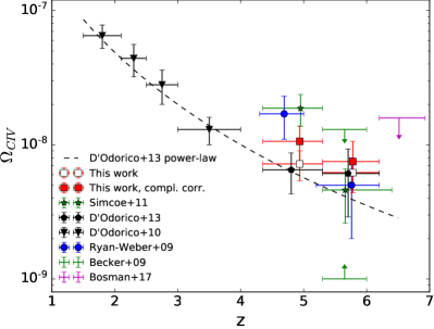
Figure 5: Evolution of the cosmic density of C IV  at $1.5\lesssim z\lesssim 6.2$ (D’Odorico et al., 2010, 2013, black triangles,black pentagons) and the corresponding power-law fit $\Omega_{\text{C{\tiny IV}}}=(2\pm 1)\times 10^{-8}[(1+z)/4]^{-3.1\pm 0.1}$ (black dotted line). Our measurements (filled and empty red squares, with and without completeness correction) are in good agreement with D’Odorico et al. (2013) as well as other previous studies: Ryan-Weber et al. (2009, blue dots), Becker et al. (2009, green $95\%$ confidence interval), Simcoe et al. (2011, dark green stars) and Bosman et al. (2017, magenta upper limit). The density error bars indicate $1\sigma$ confidence intervals.

We present our measurement on Fig. 5 alongside previous results in the literature. We chose a C IV  absorber sample with selection criteria $13.8\leq\log N_{\text{C{\tiny IV}}}<15.0$ at the two redshift intervals, $4.3<z<5.3$ and $5.3<z<6.2$, to facilitate a fair comparison with DO13’s extensive dataset across all redshifts. We note the agreement with their evolution which indicates a general decline in cosmic density with redshift. We note that although different observations and recovery pipelines differ on the exact list of absorbers between studies, the cosmic density measurements are very similar. We list the values with and without complete correction (Table 3) for different redshift intervals in Table 4. The completeness correction does not significantly change the overall decline of the cosmic density in our redshift interval.

This decline of $\Omega_{\text{C{\tiny IV}}}$ reflects both (i) the build up of total carbon budget at decreasing redshifts, as more metal is ejected into the circum-/inter-galactic medium around star-forming galaxies by outflows, and (ii) the changing ionisation state of carbon due to the evolving spectral shape of the UV background (see e.g. Becker et al., 2015, for a review and references therein). We will discuss the chemical enrichment and other properties of C IV-host in Section 5 after presenting their 1D correlation with the IGM transmission.

3.2 The observed 1D correlation of C IV  with IGM transmission

The main result of this paper is the 1D correlation between our C IV  absorbers and the IGM transmission shown in Fig. 7. We compute the correlation using Davis & Peebles (1983) estimator

$$\hat{\xi}_{\text{C{\tiny IV}}-\rm Ly\alpha}(r)=\frac{D_{\text{C{\tiny IV}}}D_{\text{T}}}{R_{\text{C{\tiny IV}}}D_{\text{T}}}-1\,=\frac{\langle T(r)\rangle_{\text{C{\tiny IV}}}}{\overline{T}}-1\text{ , }$$ (6)

where the $D_{\text{C{\tiny IV}}}$ is the pixel corresponding to the H I Lyman-$\alpha$ absorption at the redshift of a detected C IV  absorber, and $D_{T}=\langle T(r)\rangle_{\Delta r}$, is the transmission in the forest of the QSOs at a distance $r$ from the C IV  absorber. To make the comparison with previous studies easier, we provide a equivalent formulation where $\langle T(r)\rangle_{\text{C{\tiny IV}}}$ is the average Lyman-$\alpha$ transmission $T$ at a distance $r$ of the redshift C IV  absorbers, and $\overline{T}$ is the average transmission at the redshift $z$ in the QSO line-of-sight (LOS) studied. Operationally, for each $D_{\text{C{\tiny IV}}}$, we take the transmission in neighbouring pixels $D_{T}$ and compute the LOS Hubble distance. Similarly, the average transmission is estimated from a random distribution of absorbers with redshifts $R_{\text{C{\tiny IV}}}$. The random redshifts $R_{\text{C{\tiny IV}}}$ are generated by oversampling $50$ times the redshift interval $z_{\text{C{\tiny IV}}}\pm 0.1$ around each observed C IV  absorber detected at $z_{\text{C{\tiny IV}}}$ in each LOS, so as to reproduce the observed redshift distribution and sightline-to-sightline transmission variance. We note that the conversion from velocity space to Hubble distance is subject to a caveat due to peculiar velocities on small scales further discussed in Section 5.3. We weight the pixels with the inverse variance as we perform the mean to bin the correlation function linearly or logarithmically depending on the analysis, and we bin the observed and random absorbers in a consistent manner. In order to have sensible values of the transmission and correct for any misfits of the power-law continuum (see Section 2.1), we remove pixel artifacts by excluding those with $T<-2e$ and $T-e>1$, where $T$ is the transmission and $e$ the corresponding measurement error. We also only use pixels between $1045$ and $1176\,$ Å  in the QSO rest-frame to avoid the QSO Lyman-$\beta$ and -$\alpha$ intrinsic emission. To estimate the error we choose a Jackknife test given our modest sample of sightlines. We draw $500$ subsets of half of the C IV  sample, generate accordingly the random samples and compute the correlation for these subsets. The variance of the $500$ draws is then used as an estimate of our errors. We note that this method is more conservative than Poisson or bootstrap errors, and converges with an increasing sample size.

Not all C IV  absorbers detected in the sightline of the QSOs are suitable for this measurement. We define here the sample of C IV  absorbers redshifts used for the correlation with the IGM transmission, named Sample $\alpha$. First and foremost, the corresponding H I Lyman-$\alpha$ should be between $1045$ and $1176\,$ Å  in the QSO rest-frame to avoid the QSO Lyman-$\beta$ and -$\alpha$ intrinsic emission. Secondly, as we are using C IV  as a tracer of galaxies we take only the redshift of the strongest absorber for systems with multiple components when they are $\delta v<100$ km s^-1 apart. This avoids systems with multiple components multiply sampling the same part of the QSO forest and thus biasing the measurement. Finally, as our estimator requires a proper measurement of the transmission in the Lyman-$\alpha$, it cannot produce a sensible measurement where the average flux in the Lyman-$\alpha$ forest falls below the sensitivity of the spectrograph , producing lower limits on the correlation that are not easily interpreted. We hence remove C IV  absorbers lying in saturated end regions of the Lyman$-\alpha$ forest where the average transmission over $\Delta z=0.1$ is less than the average $1\sigma$ error level of the flux measurement. We emphasize that this last step only removes the end part of two QSO forests in which C IV  absorbers sit, and exclude only $\sim 10\%$ of Sample $\alpha$.

The selection described above leaves $37$ C IV  systems absorbers suitable for the correlation measurement to which we add the $z=5.738$ absorber on the LOS of J1148+3549 from Ryan-Weber et al. (2009), which was detected in a NIRSPEC spectra in wavelengths unaccessible to our ESI spectra. The average redshift of Sample $\alpha$ is $\langle z_{\text{C{\tiny IV}}}\rangle=5.18$ and the average column density $\log\langle N_{\text{C{\tiny IV}}}\rangle\simeq 13.8$. We show the 6 lower-redshift detections of Sample $\alpha$ on Fig. 6. The whole sample is presented in Appendix B.

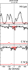
Figure 6: First lower-redshift detections of our C IV  sample detected with a corresponding H I Lyman-$\alpha$ absorption in the QSO Lyman-$\alpha$ forest. The entire sample of $37$ such absorbers is presented in Fig. 10.

The 1D correlation signal reveals an excess absorption at $r_{c}\lesssim 5$ cMpc/h around C IV  absorbers at $4.5<z<6$. This excess absorption is also found around $z\sim 3$ Lyman Break Galaxies (LBGs) (Adelberger et al., 2003, 2005; Bielby et al., 2017) (see Figure 7 for a comparison). The excess absorption is detected on the same scales ($\sim 5$ cMpc/h) for both $z\sim 3$ LBGs and $z\sim 5.2$ C IVs, but the excess absorption seems much stronger in the latter objects. The absorption excess is perhaps emerging more clearly due the overall opaqueness Lyman-$\alpha$ forest at $z\sim 5.2$. The trough also shows the expected co-spatiality of C IV  and Lyman-$\alpha$ absorption. There is also an excess of transmission at $10\lesssim r\lesssim 30$ cMpc/h around C IV . This excess on large scales was detected around spectroscopically confirmed LBGs in Paper I. The significance of the excess on $10-30$ cMpc/h scales is $2.7\sigma$ for the average transmission $T\simeq 0.14$ versus a null mean flux. We note that the signal goes to zero at large distances, indicating that the excess is unlikely to be caused by the wrong normalisation of the 1D C IV-IGM correlation. We discuss the physical implications in Section 5.

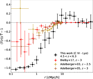
Figure 7: The measured 1D correlation between C IV  absorbers and the IGM transmission (black) is compared to previous studies on LBG-IGM correlation: Adelberger et al. (2003, 2005, yellow, orange crosses), studies at $z\sim 2.5$ and $z\sim 3$ and the VLT LBG survey at $z\sim 3$ (Bielby et al., 2017, red crosses). The central trough is enhanced at high redshift and the excess on the large scales is in contrast to the flat profile seen in low-redshift data.

4 Modelling the C IV-IGM correlation

In order to interpret the data, we use the linearised version of the model introduced and discussed in detail in Paper I. The precepts for the LBG-IGM cross-correlation discussed in Paper I can be easily modified for any tracer of galaxies, and the dense, ionised C IV  gas is an ideal candidate.

Supposing that galaxies hosted by dark matter haloes eject their material by galactic winds, chemically enriching the surrounding IGM environment. C IV  absorbers act as a tracer of galaxies. At $z\gtrsim 5$, patchy reionisation can produce the fluctuations in the UV background affecting the Ly$\alpha$ forest transmission around galaxies. Therefore, the C IV-IGM correlation will reflect both (i) the correlation between matter and galaxies and (ii) the enhanced UV background around the C IV-host galaxies. Following Appendix B of Paper I, we showed the expected flux transmission at a comoving distance $r$ from the position of a C IV  absorber is

$$T(r)=\exp(-\tau_{\alpha}(r))=\overline{T}(1+\xi_{\text{C{\tiny IV}}-\rm Ly\alpha}(r))\text{ , }$$ (7)

where $\overline{T}$ is the average transmitted flux in the Lyman-$\alpha$ forest at the redshift of interest, and the C IV-IGM correlation along the LOS is then given by

$$\xi_{\text{C{\tiny IV}}-\rm Ly\alpha}(r)\approx b_{\text{C{\tiny IV}}}b_{\alpha}\xi_{\rm m}^{\text{lin}}(r,\mu=1)+b_{\text{C{\tiny IV}}}b_{\Gamma}\xi_{\Gamma}^{\rm lin}(r)\,\text{ . }$$ (8)

The contribution of the matter correlation around galaxies is quantified with the two bias factors of C IV-host galaxies $b_{\text{C{\tiny IV}}}$ and the Lyman-$\alpha$ forest $b_{\alpha}$. The redshift-space sightline linear matter correlation function $\xi^{\rm lin}_{m}(r,\mu=1)$ follows from the real-space matter correlation function (Hamilton, 1992),

$$\xi^{\rm lin}_{m}(r,\mu=1)=\xi_{0}(r)P_{0}(\mu)+\xi_{2}(r)P_{2}(\mu)+\xi_{4}(r)P_{4}(\mu)$$ (9)

with $\xi_{0}(r)=[1+(\beta_{\text{C{\tiny IV}}}+\beta_{\alpha})/3+\beta_{\text{C{\tiny IV}}}\beta_{\alpha}/5]\xi(r)$, $\xi_{2}(r)=[(2/3)(\beta_{\text{C{\tiny IV}}}+\beta_{\alpha})+(4/7)\beta_{\text{C{\tiny IV}}}\beta_{\alpha}][\xi(r)-\bar{\xi}(r)]$, and $\xi_{4}(r)=(8/35)\beta_{\text{C{\tiny IV}}}\beta_{\alpha}[\xi(r)+(5/2)\bar{\xi}(r)-(7/2)\bar{\bar{\xi}}(r)]$ where $\xi(r)$ is the linear matter correlation function in real space, and $\beta_{\text{C{\tiny IV}}}$ and $\beta_{\alpha}$ are the redshift space distortion (RSD) parameters (Kaiser, 1987). The RSD parameter of C IV  is set to $\beta_{\text{C{\tiny IV}}}\approx\Omega_{m}^{0.6}(z)/b_{\text{C{\tiny IV}}}\approx 1/b_{\text{C{\tiny IV}}}$. The Lyman-$\alpha$ forest RSD parameter $\beta_{\alpha}$ is found to be relatively constant at lower redshift from observations in the range $\beta\simeq 1.2-1.7$ (Slosar et al., 2011; Blomqvist et al., 2015; Bautista et al., 2017). We set $\beta_{\alpha}=1.5$ as a fiducial value. The Ly$\alpha$ forest bias is chosen such that the model 1D Ly$\alpha$ forest power spectrum is consistent with observations from Viel et al. (2013), which leads to the fiducial value of $b_{\alpha}=-1.3$.

On large scales, the contribution of the enhanced UV background becomes increasingly important. The mean photoionisation rate $\bar{\Gamma}$ of the IGM from star-forming galaxies depends on the the population average of the product of LyC escape fraction and and LyC photon production efficiency $\langle f_{\rm esc}\xi_{\rm ion}\rangle$,

$$\bar{\Gamma}\propto\langle f_{\rm esc}\xi_{\rm ion}\rangle\lambda_{\rm mfp}\int^{M_{\rm UV}^{\rm lim}}_{-\infty}L_{\rm UV}(M_{\rm UV})\frac{dn}{dM_{\rm UV}}dM_{\rm UV}\text{ , }$$ (10)

where $dn/dM_{\rm UV}$ is the UV luminosity function (Bouwens et al., 2015) and $M_{\rm UV}^{\rm lim}$ is the limiting UV magnitude of galaxies that contribute to the UV background. We adopt the value of mean free path $\lambda_{\rm mfp}$ of Worseck et al. (2014). The effect of the UV background is then modelled through the bias factor $b_{\Gamma}$ defined by

$$b_{\Gamma}=\frac{\int\Delta_{b}P_{V}(\Delta_{b})\tau_{\alpha}(\bar{\Gamma},\Delta_{b})e^{-\tau_{\alpha}(\bar{\Gamma},\Delta_{b})}}{\int\Delta_{b}P_{V}(\Delta_{b})e^{-\tau_{\alpha}(\bar{\Gamma},\Delta_{b})}}\,\text{ , }$$ (11)

where $\tau_{\alpha}(\bar{\Gamma},\Delta_{b})\simeq 5.5\Delta_{b}^{2}(\bar{\Gamma}/10^{-12}{\rm s^{-1}})^{-1}(T/10^{4}{\rm K})^{-0.72}[(1+z)/6]^{9/2}$ is the Lyman-$\alpha$ optical depth at the mean photoionisation rate (we assume a uniform temperature of $T=10^{4}$ K), $P_{V}(\Delta_{b})$ is the volume-weighted probability distribution function of baryon overdensity $\Delta_{b}$ (Pawlik et al., 2009). The correlation function of the UV background with galaxies is

$$\xi_{\Gamma}^{\rm lin}(r)=\langle b_{g}(<M^{\rm lim}_{\rm UV})\rangle_{L}\int\frac{k^{2}\text{d}k}{2\pi^{2}}R(k\lambda_{\rm mfp})P^{\rm lin}_{m}(k)\frac{\sin kr}{kr}\,\text{ , }$$ (12)

where $R(k\lambda_{\rm mfp})=\arctan(k\lambda_{\rm mfp})/(k\lambda_{\rm mfp})$, $P_{m}^{\rm lin}(k)$ is the linear matter power spectrum, and $\langle b_{g}(<M_{\rm UV})\rangle_{L}$ is the luminosity-weighted bias of ionising sources above $M^{\rm lim}_{\rm UV}$, which is evaluated with the same procedure as in Paper I. We use the halo occupation number framework with the conditional luminosity function which parameters are fixed by simultaneously fitting the Bouwens et al. (2015) $z\sim 5$ luminosity function and the Harikane et al. (2016) LBG correlation functions, resulting in the best-fit parameters $(M_{\rm UV,0},\log M_{h}^{\ast},\gamma_{1},\gamma_{2},\sigma_{c},\log\phi_{0},\alpha_{s},\beta_{s})=(-22.29,11.90,2.39,-0.06,0.2\mbox{(fixed)},-1.49,-1.26,0.85)$ (see Paper I for more details).

Overall, the linear model used to describe the observed C IV-IGM correlation contains five parameters; two to describe the UV background $(\langle f_{\rm esc}\xi_{\rm ion}\rangle,M_{\rm UV}^{\rm lim})$, one to describe the halo bias of C IV-host galaxies $b_{\rm CIV}$, and two to describe the matter fluctuations in the Lyman-$\alpha$ forest $(b_{\alpha},\beta_{\alpha})$. Our fiducial linear model leaves the first three parameters free $(\langle f_{\rm esc}\xi_{\rm ion}\rangle,M_{\rm UV}^{\rm lim},b_{\text{C{\tiny IV}}})$, but the full five parameter model including $(b_{\alpha},\beta_{\alpha})$ is examined in Appendix C.

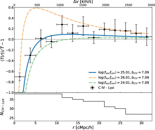
Figure 8: Upper panel: The measured correlation between C IV and the IGM transmission, linearly binned, compared to our models. We show various linear models of the correlation for illustrative purposes. Blue line (maximum likelihood model, see Fig. 9) : $(\log\langle f_{\text{esc}}\xi_{\text{ion}}\rangle/[{\rm erg^{-1}~{}Hz}]=25.01,M_{\text{UV}}^{\text{lim}}=-10.82,b_{\text{C{\tiny IV}}},b_{\alpha}=-1.3,\beta_{\alpha}=1.5)$. We then change the parameter of interest, the photon production product to show the impact on the correlation. Orange semi-dotted line: $\log\langle f_{\text{esc}}\xi_{\text{ion}}\rangle/[{\rm erg^{-1}~{}Hz}]=26.01$. Green semi-dotted line: $\log\langle f_{\text{esc}}\xi_{\text{ion}}\rangle/[{\rm erg^{-1}~{}Hz}]=24.01$. The limitation of the linear model on the scale where it produces unphysical values of $\xi_{\text{C{\tiny IV}}-{\rm Ly}\alpha}(\lesssim 3\text{cMpc/h})<-1$. In order to limit the impact on the fit, we capped the value of the linear model at $-1$ and excluded the first point from the fit. Lower panel: Number of C IV  absorbers in Sample $\alpha$ contributing to the measure at different scales.

We fit the linear model to the linearly binned correlation using the Markov chain Monte Carlo affine sampler from the emcee package (Foreman-Mackey et al., 2013). In doing so, we assume a flat prior in all three parameters in the following ranges: $23<\log\langle f_{\text{esc}}\xi_{\text{ion}}\rangle/[{\rm erg^{-1}~{}Hz}]<27$, $-20<M_{\text{UV}}^{\text{lim}}<-8$, $0<b_{\text{C{\tiny IV}}}<10^{3}$. The priors are quite broad and encompass all plausible physical values. We run the sampler for $5000$ steps with $24$ walkers, discarding $500$ steps for burn-in and fixing the scale parameter to ensure the acceptance rate stays within $0.3<r<0.5$. The walkers are initialized in a Gaussian sphere with variance $\sigma=0.1$ at different locations in the allowed parameter space, without any noticeable change to our results. We exclude the first datapoint at $r=2.5\pm 2.5$ cMpc/h from the fit and we cap the linear model at $-1$ because it does not hold on very small scales, predicting unphysical correlation values $\xi(r\lesssim 2.5\text{cMpc/h})<-1$. The model is evaluated at $\langle z_{\text{C{\tiny IV}}}\rangle=5.18$. The resulting fit and the possible inference on the three parameters is discussed in the next section.

5 Physical implications

We discuss the physical implications of our measurements of the C IV-IGM 1D correlation at $z\simeq 5$. The two main features of the correlation are (i) an excess Lyman-$\alpha$ forest absorption on small scales $r<5$ cMpc/h suggestive of the gas overdensity around C IV  absorbers and indicative evidence of the outskirt of the CGM around the $z>5$ galaxies, and (ii) an excess IGM transmission on large-scale ($r\gtrsim 10$ cMpc/h) which is consistent with an enhanced UV background around C IV  powered by galaxy clustering with a large ionising photon budget as predicted in Paper I. In Fig. 8 we show the observed C IV-IGM correlation overlaid with our linear model presented before. The large scale excess transmission of the correlation is reasonably well captured by the model despite its simplicity, confirming the foregoing interpretation. Clearly any interpretation, and subsequent inference on the exact escape fraction and spectral hardness, will be subjected to the uncertainties due to our modest sample size and theoretical model. These are addressed in Section 5.3.

We show the posterior probability distribution of the parameters for our likelihood in Fig. 9. We find that the observed large-scale IGM transmission excess requires a large population-averaged product of LyC escape fraction and spectral hardness parameter, $\log\langle f_{\text{esc}}\xi_{\text{ion}}\rangle/[{\rm erg^{-1}~{}Hz}]=25.01_{-0.19}^{+0.30}$ (for the fiducial model fit) where the quoted error is the $1\sigma$ credibility interval. Even using a conservative modelling approach using the full five parameters with flat priors, the observed level of the large-scale excess seems to indicate a large value $\log\langle f_{\text{esc}}\xi_{\text{ion}}\rangle/[{\rm erg^{-1}~{}Hz}]\gtrsim 24.7$ ($1\sigma$ limit) (see Appendix C for full details). The limiting UV magnitude of the ionising sources is unconstrained in the prior range. At face value, the best-fit value of C IV  bias $b_{\text{C{\tiny IV}}}=7.09^{+3.29}_{-2.89}$ appears somewhat large corresponding to a host halo mass of $11.3\lesssim\log M_{\rm h}/{\rm M_{\odot}}\lesssim 12.6$. However, this value is degenerate with other Lyman-$\alpha$ forest parameters unknown at $z>5.0$, permitting values as small as $b_{\text{C{\tiny IV}}}=3.5^{+2.0}_{-1.0}$. The corresponding host halo mass of $10.4\lesssim\log M_{\rm h}/{\rm M_{\odot}}\lesssim 11.6$ is then consistent with the data. Therefore, the host halo mass of C IV  absorbers is loosely constrained to lie between $10.4\lesssim\log M_{\rm h}/{\rm M_{\odot}}\lesssim 12.6$.

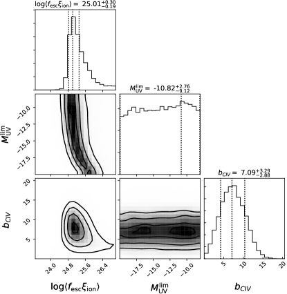
Figure 9: Posterior distribution of the parameters in our linear model of the correlation. The quoted numbers of the 1-D histogram give the $1\sigma$ credibility interval. Fitting the data with our linear model put constraints on the product $\log\langle f_{\text{esc}}\xi_{\text{ion}}\rangle/[{\rm erg^{-1}~{}Hz}]=25.01^{+0.30}_{-0.19}$ and the bias of the C IV  haloes $b_{\text{C{\tiny IV}}}=7.09^{+3.29}_{-2.86}$. The limiting UV magnitude of UV contributors is left unconstrained. It is indeed the parameter that affects the least the correlation.

5.1 The properties of C IV  hosts, faint galaxies and feedback

We can use abundance matching to compute the halo mass of the C IV  hosts. We find that the sightline number density of our sample of C IV  absorbers with $\log N_{\text{C{\tiny IV}}}>13.0$ is $\text{d}\mathcal{N}/\text{d}X=4.38\pm 0.42~{}(4.42\pm 0.85)$ for absorbers at $4.3<z<5.3\,(5.3<z<6.2)$, where the quoted errors are Poisson and we have applied a completeness correction.

We then compute the comoving density of the absorbers. As galactic outflows enrich the gas around galaxies out to a distance $R_{\text{C{\tiny IV}}}$ and with a C IV  covering fraction $f_{\rm c}$, assuming a one-to-one relation between C IV  absorbers and dark matter haloes, the incidence rate is

$$\frac{d\mathcal{N}}{dX}=\frac{c}{H_{0}}\int_{M_{\rm h}}^{\infty}\langle f_{\rm c}\pi R^{2}_{\text{C{\tiny IV}}}\rangle\frac{dn}{dM^{\prime}_{\rm h}}dM^{\prime}_{\rm h}\text{ , }$$ (13)

where $\langle f_{\rm c}\pi R^{2}_{\text{C{\tiny IV}}}\rangle$ is the population-averaged physical cross section of metal enriched gas, $dn/dM_{\rm h}$ is a halo mass function in comoving units, and the comoving density is given by $\phi\equiv\int_{M_{\rm h}}^{\infty}\frac{dn}{dM^{\prime}_{\rm h}}dM^{\prime}_{\rm h}$. A conservative maximal enrichment radius for C IV  is $r\lesssim 100$ pkpc, which has been derived from simulations of high-redshift galaxies by Oppenheimer et al. (2009). Keating et al. (2016) have found that the maximal enrichment radius could be twice as small, with most metal-rich outflows traveling less than 50 pkpc from their host galaxy. Assuming a single physical cross-section for the whole sample, we derive likely UV luminosities and masses for C IV  hosts with a conservative enrichment radius $25<R_{\text{C{\tiny IV}}}<100$ pkpc with $f_{\rm c}=1$. For our fiducial choice of $5.3<z<6.2$ absorbers, $d\mathcal{N}/dX=4.42$, and a physical cross enrichment radius of $R_{\text{C{\tiny IV}}}\simeq 100$ pkpc, we find $\phi\simeq 3.2\times 10^{-2}$ cMpc^-3.

This translates to likely halo masses of $M_{\text{h}}\gtrsim 10^{10}M_{\odot}$ (Murray et al., 2013). We can also translate the abundance to luminosities of $M_{\text{UV}}\lesssim-16$ (e.g. Bouwens et al., 2015). Clearly a smaller enrichment radius by weaker outflow and/or clumpy distribution of metal enriched gas ($f_{c}<1$) requires lower mass, more abundant haloes as the hosts of C IV . With improved measurements and analysis, in the future we hope to invert this argument such that, given an independent measure of C IV-host halo mass from the correlation, it will be possible to infer the cross-section of metal enriched gas, i.e. the properties of galactic outflows around near reionisation-era galaxies.

Our study offers an interesting new insight on C IV  absorbers as we view them in absorption with respect to the Lyman-$\alpha$ forest at $z\sim 5$. We note that all C IV  absorbers in our Sample $\alpha$ always fall into highly opaque troughs with no Lyman-$\alpha$ transmission, which is surprising given that velocity shifts can occur between the C IV  and the expected associated Lyman-$\alpha$ line, and thus in principle flux could be detected in some cases (see Fig. 6 and 10). When multiple C IV  absorbers are detected in the same trough, the separation is at least $0.002<\Delta z<0.005$. Pairs of C IV  absorbers sharing the same trough could be two distinct C IV-enriched clouds, corresponding to separations of $200-400$ ckpc/h. Alternatively this might imply outflows with speeds around $\sim 25-100$ km s^-1. The absence of Lyman-$\alpha$ transmission at the redshift of every C IV  absorber and the average separation between absorbers within the same opaque region could potentially serve as a test for models which aim at reproducing the distribution and velocity of metals in the early Universe.

5.2 Escape fraction, spectral hardness and UV background

Our inference on the mean ionising photon production rate and escape fraction product of the galaxies clustered around C IV  and likely contributing to reionisation is $\log\langle f_{\text{esc}}\xi_{\text{ion}}\rangle/[{\rm erg^{-1}~{}Hz}]=25.01^{+0.30}_{-0.19}$. This would imply a $\gtrsim 50\%$ escape fraction if adopting the “canonical” values of the LyC production efficiency of $\log\xi_{\text{ion}}/[{\rm erg^{-1}~{}Hz}]=25.2-25.4$ found for $z=4-5$ LBGs (Bouwens et al., 2016). However, recent studies of intermediate redshift Lyman-$\alpha$ Emitters (LAEs) (Nakajima et al., 2016, 2018) and CIII] emitters (Stark et al., 2015, 2017) have found higher LyC production rates in the range at $\log\xi_{\text{ion}}/[{\rm erg^{-1}~{}Hz}]\simeq 25.5-25.8$. Our estimated value for the product would still then imply a high mean escape fraction e.g. $\langle f_{\text{esc}}\rangle\simeq 0.32~{}(0.16)$ for a fiducial $\log\langle\xi_{\text{ion}}\rangle/[{\rm erg^{-1}~{}Hz}]=25.5~{}(25.8)$. Conceivably, our sub-luminous sources clustered around C IV  absorbers may have an even harder ionising spectrum if these sources are expected to have an average escape fraction of $\lesssim 10\%$ as is found at lower redshift.

In Paper I we found an escape fraction $\langle f_{\text{esc}}\rangle\gtrsim 10\%$ with a fiducial $\log\langle\xi_{\text{ion}}\rangle/[{\rm erg^{-1}~{}Hz}]=25.2$ for faint galaxies clustered around LBGs, with a $\log\langle f_{\text{esc}}\xi_{\text{ion}}\rangle$ product $1$ dex lower than our inference from the C IV-IGM 1D correlation. At face value both the escape fraction and the spectral hardness of the galaxies probed by C IV  absorbers seems to be increased with respect to the population probed by LBGs in Paper I. Meanwhile, we found several O I absorbers (Becker et al., 2006) in the vicinity of a confirmed LBGs, while none of our detected C IV  absorbers had a confirmed bright counterpart in the LOS towards J1148+5251. These two clues likely suggest that the population traced by LBGs and C IV  absorbers is different.

If C IV  systems correspond to $M_{\text{UV}}\lesssim-16$ galaxies, then by using them as tracers we are likely selecting overdensities less massive and fainter than those traced by LBGs and LAEs. A harder spectrum might then be attributed to a faint clustered population, consistent with the trend of a harder ionising spectrum $\xi_{\text{ion}}$ in fainter galaxies recently reported by Nakajima et al. (2016, 2018). We can however not exclude that a high average escape fraction is solely driving our high value of $\log\langle f_{\text{esc}}\xi_{\text{ion}}\rangle$.

Finally, our results have interesting implications for the observability of galaxies associated with C IV-hosting halos. C IV  is a highly ionised ion, indicating the presence of radiation at the $\sim$4 Ryd level in the immediate vicinity of the hosts. While at low redshift this radiation is provided by the mean UVB, at $z=5$ the large-scale excess transmission seems to indicates that the collective radiation by large-scale galaxy overdensities around C IV  absorbers becomes important. Together with our relatively large halo masses for C IV  hosts ($10.4\lesssim\log M_{\rm h}/{\rm M_{\odot}}<12.6$), this seems to indicate that C IV  absorption should be tracing galaxy overdensities. However, the independent evidence from searches for emission counterparts to metal absorbers at high redshift is sparse and conflicting (Díaz et al., 2011; Cai et al., 2017). To date, no direct emission counterparts of C IV  absorbers have been found at $z>5.0$. In spite of this, Díaz et al. (2014, 2015) found an overdensity of LAEs within 10 cMpc/h of two quasar sightlines containing C IV  absorbers. This is broadly consistent with the picture in which the strongest ionisation takes place in small galaxies, implying the likely hosts of C IV  would be fainter LAEs within overdensities of brighter objects.

5.3 Alternative interpretations and caveats

We have assumed for our analysis that C IV  absorbers are good tracers of galaxies. Due to the C IV  wind velocity and the spatial distance between the gas and the host galaxy, this assumption is however only true on somewhat large scales. The typical outflow speed (e.g. Steidel et al., 2010) is $\sim 200$ km/s, meaning that at $z\sim 5.5$, the maximum distance a metal can travel over the age of the Universe is about $\sim 0.2$ pMpc. In simulations where a more careful modelling of the distribution of metals is done, C IV  is expected to travel on average $\lesssim 100$ pkpc away from the progenitor galaxy (Oppenheimer et al., 2009; Bird et al., 2016; Keating et al., 2016). The recent detection of a galaxy at $\sim 40$ pkpc from a C IV  absorber in the sightline of J2310+1855 further strengthen this point (D’Odorico et al., 2018) . Given the expected spatial offsets ($\lesssim 0.2pMpc$), and the wind speeds involved ($\sim 200$ km/s), it is fair to argue that the redshift of C IV  is a proxy for the redshift of the host galaxy with an error $<400$ km/s. We note that this is comparable with the typical difference between the systemic redshift and the one derived from Lyman-$\alpha$ emission for galaxies in Paper I. Thus C IV  reasonably traces galaxies on scales $\gtrsim 0.6$ pMpc at redshift $z\sim 5.5$. This impacts only the two innermost bins of the correlation in Fig. 8, but the innermost bin is excluded from the fit for reasons exposed above. Hence we conclude C IV  is therefore a suitable tracer of galaxies for the purpose of the 1-D correlation with the IGM transmission where a transmission excess is expected to show a positive signal on scales much greater than the redshift-space offset between C IV  and its host ($10-30$ cMpc).

An alternative interpretation of the transmission excess seen at $r\gtrsim 10$ cMpc/h in Fig. 8 is shifted Lyman-$\alpha$ flux from a associated galaxies. This, however, would imply a mean velocity shift of $\Delta v_{\mbox{\tiny Ly}\alpha}\gtrsim 1000$ km s^-1, which is a very high value considering the results of previous studies (e.g. Adelberger et al., 2003; Steidel et al., 2010; Erb et al., 2014; Stark et al., 2017). The addition of the physical offset between C IV  gas and the progenitor galaxy could potentially add to this shift, but we have no reason to believe that spatial offsets of C IV  and velocity offsets of Lyman-$\alpha$ should conspire to influence significantly the observed flux in the Lyman-$\alpha$ forests of QSOs.

Measuring the correlation of any population with the IGM transmission is subject to uncertainties. First of all, the sample is subject to cosmic variance even with a size of $38$ objects. Indeed, some sightlines present up to $\sim 5$ C IV absorbers with $\log N_{\text{C{\tiny IV}}}>13$ where some are devoid of them in the redshift range searched (see Fig. 4). This, in conjunction with the fact that the Lyman-$\alpha$ forest at $5<z<6$ can show large deviations from the mean opacity (Bosman et al., 2018), yields a noisy correlation even with our sample.

Two other sources of errors are the possible contamination of the Lyman-$\alpha$ forest of the QSO by weak emission and/or metal absorption lines from C IV  host galaxies or nearby galaxies. The first should only contribute at most in a few bins of Fig. 8, given the $200$-$250$ km s^-1 winds of C IV clouds. As all our observations were carried out with $0.5^{\prime\prime}-1^{\prime\prime}\times 11^{\prime\prime}$ slits (XShooter) and $0.5^{\prime\prime}-1^{\prime\prime}\times 20^{\prime\prime}$ slits (ESI), the C IV  hosts most of the time do not fall in the slit if they are believed to be within $<100$ pkpc of the C IV  cloud. We hence expect no significant contamination from an associated Lyman-$\alpha$ emitting galaxy in the QSO Lyman-$\alpha$ forest. Metal absorption lines (e.g. Si III $1206$) can only reduce the signal observed and thus would not affect our claimed excess transmission on large scales. The large redshift interval sampling is likely to smear the signal as there may be a rapid evolution in the population of C IVat $z\sim 5$. If C IV  traces many distinct populations at once, the signal could be indeed mixed across species and redshifts, but the detection of an excess transmission still holds.

Although surprisingly effective for a first interpretation of the C IV-IGM correlation, our model has a number of shortcomings. It is firstly a linear model and thus the small scales may contain in large modelling uncertainties due to nonlinear effects. This shortcoming on the small scales is probably best illustrated by the unphysical values derived in the $r\lesssim 2.5$ cMpc/h region. This model also requires a measurement of the bias and RSD parameter of the Lyman-$\alpha$ forest at $z\gtrsim 5$. To illustrate this, we have left $b_{\alpha},\beta_{\alpha}$ as a free parameter with flat prior in $-3<b_{\alpha}<0,3<\beta_{\alpha}<0$ to see the effect on the inferred parameters (see Appendix C). We notice that $b_{\alpha}$ is in near perfect degeneracy with $b_{\text{C{\tiny IV}}}$ and $\log\langle f_{\text{esc}}\xi_{\text{ion}}\rangle$. Although the inferred $\log\langle f_{\text{esc}}\xi_{\text{ion}}\rangle$ using a flat prior is consistent within $1\sigma$ of our result presented above, a substantial uncertainty still remains. This linear model would hence benefit from a reliable measurement of the Lyman-$\alpha$ bias parameters at $z>5$. Clearly one possible way to circumvent this issue is to directly compare the 1D correlation measurement with hydrodynamical (radiative transfer) simulations calibrated against Lyman-$\alpha$ forest observables at the same redshift. We are planning to investigate such approach in future work, but we here limit ourselves to the linear model for the sake of brevity.

6 Conclusion and future work

The 1D correlation of metals with the IGM transmission offers a promising tool to test different models of reionisation and requires high-resolution spectroscopy of a fair number of bright sources at the redshift of interest. This measurement enables the indirect study of objects aligned with and hence outshined by $z\sim 6$ QSO. We have therefore conducted a semi-automated search for C IV absorbers in order to study how these absorbers can trace potential sources of ionising photons and gathered the largest sample of C IV  absorbers at $4.3<z<6.2$. We have updated the measurements of C IV cosmic density, confirming its rapid decline with redshift. Through abundance-matching arguments, we have identified C IV  as being associated with $M_{\rm UV}\lesssim-16$ faint galaxies in $\log M_{h}/{\rm M_{\odot}}\gtrsim 10$ haloes.

We have detected excess H I absorption in the Lyman-$\alpha$ forest at the redshift of $z\sim 5-6$ C IV absorbers, at a similar scale to that of the IGM absorption around lower redshift LBGs. We have also detected an excess transmission at $2.7\sigma$ on larger scales in the correlation of C IV  with the IGM transmission. We interpret this excess as a signal of the reionisation process driven by galaxies clustered around C IV  absorbers. Using the model developed in Paper I, we have put constraints on the product of the escape fraction and the LyC photon production efficiency $\log\langle f_{\text{esc}}\xi_{\text{ion}}\rangle=25.01^{+0.30}_{-0.19}$. Although caveats about the observation and the modelling remain, we have shown that C IV  absorbers trace different galaxies than the ones clustered around LAEs (Paper I), with either higher spectral hardness or possibly larger escape fractions.

More QSO sightlines are needed to fully sample cosmic variance and provide a better measurement of the correlation. Larger numbers of sightlines and absorbers would not only improve the statistics but also allow a study of the redshift evolution of the escape fraction and LyC production efficiency of the probed galaxies. We point out that a decrease of the cosmic density of C IV makes it more difficult to trace the same objects at all redshifts. However at higher redshift different metal absorbers such as Mg II or Si IV could be used to trace galaxies. In doing so, we would probe as well different ionising environments and possibly different galaxy populations. Eventually, the degeneracy with the spectral hardness of our measurement can be broken by harvesting our large sample of aligned metal absorbers to probe their ionisation state using forward modeling. Radiative transfer simulations with non-uniform UVB including the tracking and modelling of the different metal gas phases could reproduce the correlation, provided large enough boxes and sightlines can be produced in a reasonable amount of time. This opens new avenues into the question driving this series: the nature of the sources of reionisation.

Appendix A Properties of all retrieved C IV systems

We hereby give the tabulated fitted redshift, column density, Doppler parameter and the corresponding errors of all our detected C IV  absorbers in each QSO sightline studied.

Table 5: Complete list of C IV absorbers with redshift, Doppler parameter $b\,[\text{km s}^{-1}]$, column density $\log N\,[\text{cm}^{-2}]$ and associated errors.Fixed parameters in VPFIT are indicated with a ^†.

QSO	$z$	$\Delta z$	$b$	$\Delta b$	$\log N$	$\Delta\log N$
J0002+2550
	4.434586	0.000101	43.31	10.31	13.317	0.054
	4.440465	0.000091	31.22	8.24	13.696	0.049
	4.441937	0.000077	21.93	7.62	13.708	0.042
	4.675162	0.000042	8.22	7.25	13.184	0.099
	4.870726	0.000066	21.65	7.59	13.579	0.031
	4.872056	0.000097	5.74	3.19	13.498	0.208
	4.873713	0.000102	6.00†	–	13.109	0.080
	4.941568†	-	10.87	9.71	13.387	0.117
	4.943826	0.000090	5.00	4.16	13.356	0.267
	4.945804 †	-	43.39	10.10	13.417	0.051
	5.282356	0.000070	19.67	8.62	13.709	0.069
J0005-0006
	4.735463	0.000114	83.32	8.75	13.944	0.035
	4.812924	0.000088	6.64	3.67	13.832	0.400
J0050+3445
	4.724040	0.000057	9.78	5.43	13.664	0.178
	4.726409	0.000043	38.82	4.01	13.979	0.024
	4.824044	0.000090	51.15	7.91	13.763	0.040
	4.908403	0.000140	24.06	16.53	13.559	0.087
	5.221126	0.000196	31.09	19.24	13.935	0.132
J0100+2802
	4.875143	0.000119	44.59	9.08	13.218	0.065
	5.109066	0.000122	73.39	5.95	14.321	0.037
	5.111580	0.000412	49.73	30.36	13.530	0.255
	5.113629	0.000050	18.18	4.71	13.639	0.046
	5.338458	0.000059	42.39	3.94	13.955	0.033
	5.797501	0.000184	58.14	13.37	13.118	0.072
	5.975669	0.000158	20.63	13.10	12.742	0.120
	6.011654	0.000268	73.94	16.94	13.488	0.078
	6.184454	0.000362	31.35	22.12	13.061	0.256
	6.187095	0.000121	64.42	7.57	13.971	0.039
J0148+0600
	4.515751	0.000067	17.57	7.02	12.982	0.078
	4.571214	0.000090	23.70	8.34	13.060	0.087
	4.932220	0.000915	40.41	28.81	13.614	1.591
	5.023249	0.000056	6.00†	-	13.811	0.189
	5.124792	0.000042	27.09	3.02	14.084	0.039
J0231-0728
	4.138342	0.000017	9.32	2.88	13.315	0.037
	4.225519	0.000069	40.31	6.24	13.283	0.046
	4.267255	0.000063	28.12	6.14	13.200	0.053
	4.506147	0.000067	18.27	7.42	13.093	0.068
	4.569167	0.000224	93.48	16.61	13.407	0.066
	4.744957	0.000130	78.70	9.93	13.552	0.044
	4.883691	0.000205	111.96	14.74	13.566	0.048
	5.335394	0.000240	56.00	16.76	13.299	0.102
	5.357714	0.000044	28.37	3.55	13.749	0.031
	5.345812	0.000088	25.35	6.99	13.361	0.068
	5.348184	0.000043	21.49	3.75	13.647	0.038
J0353+0104
	4.675911	0.000078	21.61	12.12	13.638	0.063
	4.977485	0.000124	10.81	6.33	14.158	0.481
	5.036105	0.000454	15.00†	-	13.465	0.232
	5.037794	0.000222	15.00†	-	13.933	0.158
J0818+1722
	4.552517	0.000102	24.98	10.16	12.812	0.090
	4.620602	0.000073	25.99	6.99	13.048	0.062
	4.627338	0.000104	38.92	8.89	13.057	0.067
	4.727010	0.000068	31.70	3.07	14.005	0.065
	4.725780	0.000182	42.07	8.27	13.763	0.112
	4.731844	0.000033	41.16	2.57	13.672	0.020
	4.877661	0.000070	38.94	5.70	13.215	0.043
	4.936947	0.000107	32.24	9.12	12.666	0.075
	4.940176	0.000056	14.41	7.43	12.773	0.057
	4.941255	0.000071	10.00†	-	12.783	0.071
	4.942578	0.000060	40.13	5.22	13.188	0.036
	5.064643	0.000207	68.13	16.13	13.484	0.081
	5.076455	0.000082	33.61	6.51	13.563	0.056
	5.082651	0.000078	37.51	5.90	13.546	0.047
	5.308823	0.000061	16.45	6.50	13.031	0.054
	5.322429	0.000121	29.38	9.91	13.341	0.084
	5.789525	0.000111	38.43	7.49	13.339	0.062
	5.843998	0.000110	44.91	7.41	13.345	0.051
	5.877228	0.000106	39.41	7.26	13.315	0.055

Table 6: continued

Complete list of C IV absorbers and measured properties QSO $z$ $\Delta z$ $b$ $\Delta b$ $\log N$ $\Delta\log N$ J0836+0054 4.682130 0.000093 50.92 7.82 13.406 0.049 4.684465 0.000046 40.42 4.38 13.608 0.033 4.686503 0.000029 33.65 2.53 13.689 0.022 4.773175 0.000389 96.43 31.27 13.135 0.113 4.996702 0.000042 27.12 3.50 13.569 0.035 5.125071 0.000126 44.86 7.84 13.729 0.067 5.127266 0.000066 13.81 7.10 13.246 0.072 5.322763 0.000070 23.54 5.46 13.400 0.059 J0840+5624 4.486724 0.000060 16.99 9.88 13.674 0.096 4.525773 0.000144 52.80 14.54 13.519 0.058 4.546597 0.000021 30.20 4.36 15.395 0.384 J0927+2001 4.471037 0.000031 13.02 3.60 13.369 0.042 4.623510 0.000149 61.15 5.56 13.592 0.076 4.624132 0.000066 20.94 8.47 13.154 0.190 5.014445 0.000110 19.23 9.63 13.560 0.114 5.016426 0.000216 46.85 16.71 13.449 0.116 5.149170 0.000799 75.01 39.93 13.377 0.271 5.151154 0.000204 41.88 13.54 13.498 0.219 5.671001 0.000187 57.11 12.31 13.540 0.073 J1022+2252 5.264299 0.000152 52.66 12.47 14.410 0.078 J1030+0524 4.890614 0.000164 14.31 20.24 13.081 0.162 4.947967 0.000222 82.22 15.03 13.738 0.075 4.948468 0.000068 7.89 7.27 13.589 0.245 5.110703 0.000664 117.36 34.50 14.023 0.143 5.517461 0.000102 53.31 6.76 13.904 0.045 5.724374 0.000044 51.29 2.53 14.543 0.029 5.741183 0.000102 50.90 6.96 13.748 0.044 5.744256 0.000062 39.49 4.31 13.853 0.033 5.966889 0.000076 16.27 7.02 13.569 0.074 J1044-0125 4.450487 0.000027 14.28 3.52 13.456 0.035 4.898284 0.000188 78.05 9.81 13.759 0.060 4.899596 0.000035 13.63 5.40 13.612 0.060 5.075408 0.000091 14.12 9.69 13.433 0.107 5.077315 0.000042 26.74 3.42 13.847 0.033 5.167313 0.000055 10.59 6.40 13.493 0.099 5.285046 0.000147 36.47 11.42 13.477 0.089 5.481678 0.000080 22.20 6.70 13.775 0.070 J1048+4637 4.709835 0.000057 25.08 5.33 13.520 0.050 4.888006 0.000062 20.29 6.25 13.401 0.058 4.889219 0.000058 10.29 8.04 13.318 0.083 J1137+3549 4.781802 0.000182 50.43 17.36 13.622 0.072 4.841312 0.000108 53.00 10.08 14.005 0.042 4.874166 0.000134 74.27 10.78 14.033 0.044 J1148+5251 4.919028 0.000058 24.72 4.66 13.192 0.049 4.944227 0.000058 8.91 1.09 17.656 0.123 4.945228 0.000067 9.85 4.14 14.480 0.526 5.152113 0.000121 54.16 8.94 13.695 0.055 J1306+0356 4.613924 0.000790 103.30 31.35 13.250 0.225 4.614603 0.000033 29.33 3.21 13.722 0.050 4.615828 0.000045 23.36 4.28 13.465 0.075 4.668109 0.000020 8.71 1.87 13.993 0.115 4.668741 0.000081 56.99 4.05 13.892 0.035 4.711108 0.000135 35.60 11.23 13.129 0.096 4.860508 0.000044 35.43 3.46 13.952 0.031 4.862256 0.000055 28.31 5.49 13.933 0.051 4.863239 0.000043 10.18 3.83 13.881 0.091 4.864687 0.000053 56.14 5.04 14.327 0.026 4.866813 0.000025 20.73 2.13 14.009 0.029 4.868951 0.000102 51.40 8.62 13.670 0.055 4.880126 0.000061 27.59 4.35 13.873 0.047 4.881271 0.000058 17.01 4.23 13.690 0.061

Table 7: continued

Complete list of C IV absorbers and measured properties QSO $z$ $\Delta z$ $b$ $\Delta b$ $\log N$ $\Delta\log N$ J1319+0950 4.653406 0.000076 33.18 6.20 12.989 0.058 4.660650 0.000108 42.92 7.70 13.310 0.088 4.663610 0.000734 86.53 46.22 13.625 0.283 4.665107 0.000104 38.60 17.21 13.328 0.456 4.716591 0.000030 27.60 2.58 13.554 0.026 5.264302 0.000095 25.20 7.48 13.181 0.079 5.335365 0.000056 3.30 2.64 13.333 0.367 5.374931 0.000054 16.59 4.79 13.447 0.057 5.570341 0.000425 51.95 27.03 13.793 0.183 5.573751 0.000240 49.18 14.23 14.139 0.111 J1411+1217 4.930500 0.000439 211.93 26.04 13.982 0.048 4.960547 0.000100 6.41 4.33 13.715 0.364 5.250460 0.000063 73.55 4.62 14.442 0.025 J1509-1749 4.641643 0.000051 26.96 4.46 13.514 0.042 4.791660 0.000166 51.38 12.64 13.439 0.082 4.815429 0.000055 44.63 3.79 14.050 0.037 J2054-0005 4.868746 0.000079 15.81 8.89 13.804 0.143 5.213101 0.000147 8.67 5.96 13.828 0.368 J2315-0023 4.897117 0.001163 55.02 64.70 13.598 0.478 4.898876 0.000354 31.61 22.67 13.854 0.257

Appendix B Velocity plots of C IV absorbers used in the correlation measurement

We present in Fig. 10 the velocity for the $37$ C IV  systems of Sample $\alpha$. Note the consistent presence of at least of a few completely opaque pixels at the location where the Lyman-$\alpha$ absorption at the redshift of C IV  is expected. Note that we have not plotted individual detections of systems with less than $\lesssim 100$ km s^-1 separation as only one redshift for the whole system was retained for the correlation measurement. However, multiple absorbers forming a system but can be easily spotted on some plots.

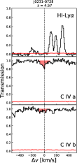
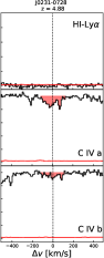
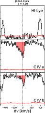
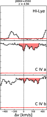
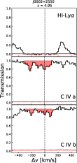
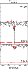
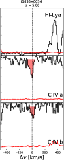
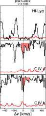
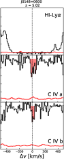
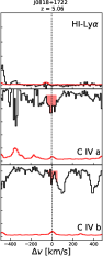
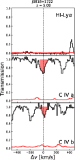
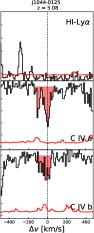
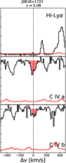
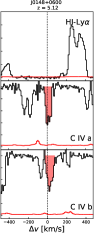
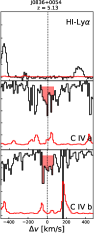
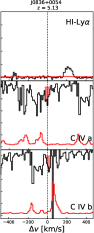
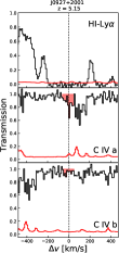
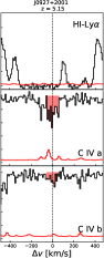
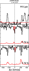
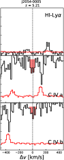
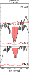
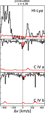
Figure 10: Velocity plots of C IV absorbers in Sample $\alpha$. For simplicity, absorbers with $\Delta v\lesssim 100$ km s^-1 were not plotted twice. They can be however be easily spotted in the lower C IV panels. All C IV absorbers land in a Lyman-$\alpha$ opaque region, often enclosed by high transmission spikes.

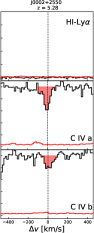
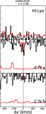
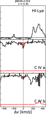
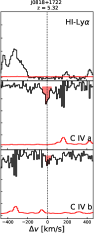
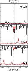
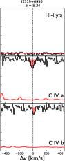
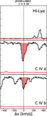
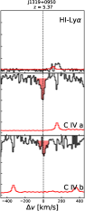
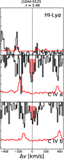
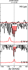
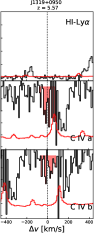
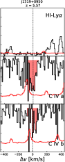
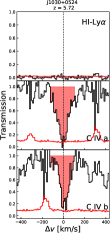
Figure 11: continued

Appendix C Relaxing the bias parameters of the Lyman-$\alpha$ forest

We present the posterior probability distribution of the parameters of our linear model including the bias of the Lyman-$\alpha$ and the associated RSD parameter as free parameters with flat priors in $-3<b_{\alpha}<0$ and $-3<\beta_{f}<0$, respectively. The result is presented in Fig. 12. The bias is in a degenerate state with all other parameters, parameters can be tuned to compensate the bias parameter changes and still produce the same fit to the data. We note that higher values of the bias than the one extrapolated from low-redshift measurements would yield in turn lower values of the host halo mass, and lower values of the escape fractions and LyC photon production product (see Table 8).

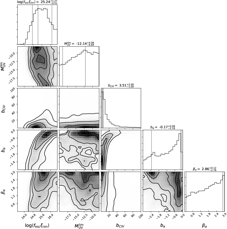
Figure 12: Posterior distribution for the $3$ original parameters of the linear model to which have been added the Lyman-$\alpha$ bias parameters $(b_{\alpha},\beta_{\alpha})$ with appropriate priors. The quoted numbers give the best-fit (maximum likelihood) and the 1-$\sigma$ credibility intervals on the marginalized distributions. The constraints on $\langle f_{\text{esc}}\xi_{\text{ion}}\rangle$ and $b_{\text{C{\tiny IV}}}$ are in good agreement with the more restricted fit presented in the main text (Fig.9). There is a clear degeneracy between these two parameters and $b_{\alpha}$. A wide variety of combinations of the $4$ parameters (excluding $M_{\text{UV}}^{\text{lim}}$) can produce a similar fit the data. Hence a choice of $(b_{\alpha},\beta_{\alpha})$ must be made in order to infer the remaining parameters.

Table 8: Inferred model parameters for different choices of Lyman-$\alpha$ bias parameters $(b_{\alpha},\beta_{\alpha})$. Notably, the choice of $b_{\alpha}=-1.3$ corresponds to our fiducial choice on the Lyman-$\alpha$ power spectrum measurement whereas $b_{\alpha}=-0.75$ corresponds the extrapolation of the evolution of the bias from low-redshift values (McDonald et al., 2006; du Mas des Bourboux et al., 2017).

$b_{\alpha}$	$\beta_{\alpha}$	$\log\langle f_{\text{esc}}\xi_{\text{ion}}\rangle$	$M_{\text{UV}}^{\text{lim}}$	$b_{\text{C{\tiny IV}}}$
-0.5	1.0	$25.55^{+0.14}_{-0.11}$	$-11.66^{+3.47}_{-8.16}$	$22.15_{-8.29}^{+7.26}$
-0.5	1.5	$25.66^{+0.21}_{-0.19}$	$-9.98^{+1.92}_{-9.96}$	$18.48_{-5.75}^{+7.67}$
-0.5	2.0	$25.66^{+0.32}_{-0.14}$	$-8.90^{+0.84}_{-10.92}$	$16.65_{-5.92}^{+6.38}$
-0.75	1.0	$25.25^{+0.19}_{-0.09}$	$-19.94^{+11.87}_{-0.00}$	$11.89_{-4.96}^{+7.80}$
-0.75	1.5	$25.35^{+0.23}_{-0.11}$	$-19.58^{+11.40}_{-0.36}$	$15.96_{-8.04}^{+2.25}$
-0.75	2.0	$25.54^{+0.22}_{-0.22}$	$-8.78^{+0.72}_{-11.16}$	$8.97_{-2.84}^{+7.95}$
-1.3	1.0	$24.92^{+0.23}_{-0.15}$	$-10.22^{+2.16}_{-9.72}$	$8.01_{-3.72}^{+2.84}$
-1.3	1.5	$25.01^{+0.30}_{-0.19}$	$-10.82^{+2.76}_{-9.12}$	$7.09_{-2.86}^{+3.29}$
-1.3	2.0	$25.17^{+0.28}_{-0.22}$	$-8.06^{+0.00}_{-11.88}$	$6.40_{-2.15}^{+2.69}$
-2.0	1.0	$24.63^{+0.15}_{-0.15}$	$-8.06^{+0.00}_{-11.87}$	$4.46_{-2.07}^{+2.85}$
-2.0	1.5	$24.80^{+0.22}_{-0.26}$	$-8.78^{+0.72}_{-11.16}$	$4.33_{-2.20}^{+1.95}$
-2.0	2.0	$24.74^{+0.55}_{-0.10}$	$-11.90^{+3.84}_{-8.04}$	$4.02_{-1.58}^{+1.69}$

References

- Adelberger et al. (2003) Adelberger, K. L., Steidel, C. C., Shapley, A. E., & Pettini, M. 2003, ApJ, 584, 45
- Adelberger et al. (2005) Adelberger, K. L., Shapley, A. E., Steidel, C. C., et al. 2005, ApJ, 629, 636
- Asplund et al. (2009) Asplund, M., Grevesse, N., Sauval, A. J., & Scott, P. 2009, ARA&A, 47, 481
- Atek et al. (2015) Atek, H., Richard, J., Jauzac, M., et al. 2015, ApJ, 814, 69
- Atek et al. (2018) Atek, H., Richard, J., Kneib, J.-P., & Schaerer, D. 2018, arXiv:1803.09747
- Bañados et al. (2016) Bañados, E., Venemans, B. P., Decarli, R., et al. 2016, ApJS, 227, 11
- Bañados et al. (2018) Bañados, E., Venemans, B. P., Mazzucchelli, C., et al. 2018, Nature, 553, 473
- Bautista et al. (2017) Bautista, J. E., Vargas-Magaña, M., Dawson, K. S., et al. 2017, arXiv:1712.08064
- Bird et al. (2016) Bird, S., Rubin, K. H. R., Suresh, J., & Hernquist, L. 2016, MNRAS, 462, 307
- Becker et al. (2015) Becker, G. D., Bolton, J. S., & Lidz, A. 2015, Publ. Astron. Soc. Australia, 32, e045
- Becker et al. (2011) Becker, G. D., Sargent, W. L. W., Rauch, M., & Calverley, A. P. 2011, ApJ, 735, 93
- Becker et al. (2012) Becker, G. D., Sargent, W. L. W., Rauch, M., & Carswell, R. F. 2012, ApJ, 744, 91
- Becker et al. (2018) Becker, G. D., Davies, F. B., Furlanetto, S. R., et al. 2018, arXiv:1803.08932
- Becker et al. (2015) Becker, G. D., Bolton, J. S., Madau, P., et al. 2015, MNRAS, 447, 3402
- Becker et al. (2009) Becker, G. D., Rauch, M., & Sargent, W. L. W. 2009, ApJ, 698, 1010
- Becker et al. (2006) Becker, G. D., Sargent, W. L. W., Rauch, M., & Simcoe, R. A. 2006, ApJ, 640, 69
- Bielby et al. (2017) Bielby, R. M., Shanks, T., Crighton, N. H. M., et al. 2017, MNRAS, 471, 2174
- Blomqvist et al. (2015) Blomqvist, M., Kirkby, D., Bautista, J. E., et al. 2015, J. Cosmology Astropart. Phys., 11, 034
- Boksenberg & Sargent (2015) Boksenberg, A., & Sargent, W. L. W. 2015, ApJS, 218, 7
- Bosman et al. (2017) Bosman, S. E. I., Becker, G. D., Haehnelt, M. G., et al. 2017, MNRAS, 470, 1919
- Bosman et al. (2018) Bosman, S. E. I., Fan, X., Jiang, L., et al. 2018, MNRAS, 479, 1055
- Bouwens et al. (2007) Bouwens, R. J., Illingworth, G. D., Franx, M., & Ford, H. 2007, ApJ, 670, 928
- Bouwens et al. (2015) Bouwens, R. J., Illingworth, G. D., Oesch, P. A., et al. 2015, ApJ, 803, 34
- Bouwens et al. (2015) Bouwens, R. J., Illingworth, G. D., Oesch, P. A., et al. 2015, ApJ, 811, 140
- Bouwens et al. (2016) Bouwens, R. J., Smit, R., Labbé, I., et al. 2016, ApJ, 831, 176
- Cai et al. (2017) Cai, Z., Fan, X., Dave, R., Finlator, K., & Oppenheimer, B. 2017, ApJ, 849, L18
- Carnall et al. (2015) Carnall, A. C., Shanks, T., Chehade, B., et al. 2015, MNRAS, 451, L16
- Carswell & Webb (2014) Carswell, R. F., & Webb, J. K. 2014, Astrophysics Source Code Library, ascl:1408.015
- Chardin et al. (2017) Chardin, J., Puchwein, E., & Haehnelt, M. G. 2017, MNRAS, 465, 3429
- Codoreanu et al. (2018) Codoreanu, A., Ryan-Weber, E. V., García, L. Á., et al. 2018, arXiv:1809.05813
- Cooper et al. (2015) Cooper, T. J., Simcoe, R. A., Cooksey, K. L., O’Meara, J. M., & Torrey, P. 2015, ApJ, 812, 58
- Crighton et al. (2011) Crighton N. H. M. et al. 2011, MNRAS, 414, 28
- D’Aloisio et al. (2017) D’Aloisio, A., Upton Sanderbeck, P. R., McQuinn, M., Trac, H., & Shapiro, P. R. 2017, MNRAS, 468, 4691
- Davies et al. (2018) Davies, F. B., Hennawi, J. F., Bañados, E., et al. 2018, arXiv:1802.06066
- De Rosa et al. (2011) De Rosa, G., Decarli, R., Walter, F., Fan, X., et al., 2011, ApJ, 739, 56
- Díaz et al. (2011) Díaz, C. G., Ryan-Weber, E. V., Cooke, J., Pettini, M., & Madau, P. 2011, MNRAS, 418, 820
- Díaz et al. (2014) Díaz, C. G., Koyama, Y., Ryan-Weber, E. V., et al. 2014, MNRAS, 442, 946
- Díaz et al. (2015) Díaz, C. G., Ryan-Weber, E. V., Cooke, J., Koyama, Y., & Ouchi, M. 2015, MNRAS, 448, 1240
- D’Odorico et al. (2010) D’Odorico, V., Calura, F., Cristiani, S., & Viel, M. 2010, MNRAS, 401, 2715
- D’Odorico et al. (2011) D’Odorico, V., Cupani, G., Cristiani, S., Maiolino, et al. 2011, Astronomische Nachrichten, 332, 315
- D’Odorico et al. (2013) D’Odorico, V., Cupani, G., Cristiani, S., et al. 2013, MNRAS, 435, 1198 (DO13)
- D’Odorico et al. (2018) D’Odorico, V., Feruglio, C., Ferrara, A., et al. 2018, ApJ, 863, L29
- du Mas des Bourboux et al. (2017) du Mas des Bourboux, H., Le Goff, J.-M., Blomqvist, M., et al. 2017, A&A, 608, A130
- Eilers et al. (2017) Eilers, A.-C., Davies, F. B., Hennawi, J. F., et al. 2017, ApJ, 840, 24
- Ellis et al. (2013) Ellis, R. S., McLure, R. J., Dunlop, J. S., et al. 2013, ApJ, 763, L7
- Erb et al. (2014) Erb, D. K., Steidel, C. C., Trainor, R. F., et al. 2014, ApJ, 795, 33
- Fan et al. (2004) Fan, X., Hennawi, J. F., Richards, Gordon T., Strauss, M. A., et al. 2004, AJ, 128, 515
- Fan et al. (2006) Fan, X., Strauss, M. A., Becker, R. H., et al. 2006, AJ, 132, 117
- Finlator et al. (2018) Finlator, K., Keating, L., Oppenheimer, B. D., Davé, R., & Zackrisson, E. 2018, arXiv:1805.00099
- Ford et al. (2013) Ford, A. B., Oppenheimer, B. D., Davé, R., et al. 2013, MNRAS, 432, 89
- Foreman-Mackey et al. (2013) Foreman-Mackey, D., Hogg, D. W., Lang, D., & Goodman, J. 2013, PASP, 125, 306
- García et al. (2017) García, L. A., Tescari, E., Ryan-Weber, E. V., & Wyithe, J. S. B. 2017, MNRAS, 469, L53
- Giallongo et al. (2015) Giallongo, E., Grazian, A., Fiore, F., et al. 2015, A&A, 578, A83
- Gill et al. (2004) Gill, S. P. D., Knebe, A., & Gibson, B. K. 2004, MNRAS, 351, 399
- Gunn & Peterson (1965) Gunn, J. E., & Peterson, B. A. 1965, ApJ, 142, 1633
- Hamilton (1992) Hamilton, A. J. S. 1992, ApJ, 385, L5
- Harikane et al. (2018) Harikane, Y., Ouchi, M., Shibuya, T., et al. 2017, ApJ, 859, 84
- Harikane et al. (2016) Harikane, Y., Ouchi, M., Ono, Y., et al. 2016, ApJ, 821, 123
- Horne (1986) Horne, K. 1986, PASP, 98, 609
- Ishigaki et al. (2015) Ishigaki, M., Kawamata, R., Ouchi, M., et al. 2015, ApJ, 799, 12
- Ishigaki et al. (2018) Ishigaki, M., Kawamata, R., Ouchi, M., et al. 2018, ApJ, 854, 73
- Izotov et al. (2016) Izotov, Y. I., Schaerer, D., Thuan, T. X., et al. 2016, MNRAS, 461, 3683
- Izotov et al. (2018) Izotov, Y. I., Schaerer, D., Worseck, G., et al. 2018, MNRAS, 474, 4514
- Jiang et al. (2016) Jiang, L., McGreer, I. D., Fan, X., et al. 2016, ApJ, 833, 222
- Kaiser (1987) Kaiser, N. 1987, MNRAS, 227, 1
- Kaiser et al. (2010) Kaiser, N., Burgett, W., Chambers, K., et al. 2010,
- Kakiichi et al. (2018) Kakiichi, K., Ellis, R. S., Laporte, N., et al. 2018, MNRAS, 479, 43, in press. (Paper I)
- Katz et al. (2018) Katz, H., Kimm, T., Haehnelt, M., et al. 2018, MNRAS, 478, 4986
- Keating et al. (2016) Keating, L. C., Puchwein, E., Haehnelt, M. G., Bird, S., & Bolton, J. S. 2016, MNRAS, 461, 606
- Kelson (2003) Kelson, D. D. 2003, PASP, 115, 688
- Knollmann & Knebe (2009) Knollmann, S. R., & Knebe, A. 2009, ApJS, 182, 608
- Kulkarni et al. (2018) Kulkarni, G., Keating, L. C., Haehnelt, M. G., et al. 2018, arXiv:1809.06374
- Landy & Szalay (1993) Landy, S. D., & Szalay, A. S. 1993, ApJ, 412, 64
- Laporte et al. (2017a) Laporte, N., Nakajima, K., Ellis, R. S., et al. 2017, ApJ, 851, 40
- Laporte et al. (2017b) Laporte, N., Ellis, R. S., Boone, F., et al. 2017, ApJ, 837, L21
- Laporte et al. (2015) Laporte, N., Streblyanska, A., Kim, S., et al. 2015, A&A, 575, A92
- Livermore et al. (2017) Livermore, R. C., Finkelstein, S. L., & Lotz, J. M. 2017, ApJ, 835, 113
- Matsuoka et al. (2016) Matsuoka, Y., Onoue, M., Kashikawa, N., et al. 2016, ApJ, 828, 26
- Matthee et al. (2017) Matthee, J., Sobral, D., Darvish, B., et al. 2017, MNRAS, 472, 772
- McDonald et al. (2006) McDonald, P., Seljak, U., Burles, S., et al. 2006, ApJS, 163, 80
- McGreer et al. (2015) McGreer, I. D., Mesinger, A., & D’Odorico, V. 2015, MNRAS, 447, 499
- McGreer et al. (2011) McGreer, I. D., Mesinger, A., & Fan, X. 2011, MNRAS, 415, 3237
- McLeod et al. (2015) McLeod, D. J., McLure, R. J., Dunlop, J. S., et al. 2015, MNRAS, 450, 3032
- McLure et al. (2009) McLure, R. J., Cirasuolo, M., Dunlop, J. S., Foucaud, S., & Almaini, O. 2009, MNRAS, 395, 2196
- Mesinger (2010) Mesinger, A. 2010, MNRAS, 407, 1328
- Mortlock et al. (2009) Mortlock, D. J., Patel, M., Warren, S. J., et al. 2009, A&A, 505, 97
- Mortlock et al. (2011) Mortlock, D. J., Warren, S. J., Venemans, B. P., et al. 2011, Nature, 474, 616
- Murray et al. (2013) Murray, S. G., Power, C., & Robotham, A. S. G. 2013, Astronomy and Computing, 3, 23
- Ouchi et al. (2018) Ouchi, M., Harikane, Y., Shibuya, T., et al. 2018, PASJ, 70, S13
- Oppenheimer et al. (2009) Oppenheimer, B. D., Davé, R., & Finlator, K. 2009, MNRAS, 396, 729
- Nakajima et al. (2016) Nakajima, K., Ellis, R. S., Iwata, I., et al. 2016, ApJ, 831, L9
- Nakajima et al. (2018) Nakajima, K., Fletcher, T., Ellis, R. S., Robertson, B. E., & Iwata, I. 2018, MNRAS, 477, 2098
- Ono et al. (2012) Ono, Y., Ouchi, M., Mobasher, B., et al. 2012, ApJ, 744, 83
- Ota et al. (2018) Ota, K., Venemans, B. P., Taniguchi, Y., et al. 2018, ApJ, 856, 109
- Parsa et al. (2018) Parsa, S., Dunlop, J. S., & McLure, R. J. 2018, MNRAS, 474, 2904
- Davis & Peebles (1983) Davis, M., & Peebles, P. J. E. 1983, ApJ, 267, 465
- Pawlik et al. (2009) Pawlik, A. H., Schaye, J., & van Scherpenzeel, E. 2009, MNRAS, 394, 1812
- Pontzen et al. (2013) Pontzen, A., Roškar, R., Stinson, G., & Woods, R. 2013, Astrophysics Source Code Library, ascl:1305.002
- Planck Collaboration et al. (2016) Planck Collaboration, Ade, P. A. R., Aghanim, N., et al. 2016, A&A, 594, A13
- Poudel et al. (2018) Poudel, S., Kulkarni, V. P., Morrison, S., et al. 2018, MNRAS, 473, 3559
- Puchwein et al. (2018) Puchwein, E., Haardt, F., Haehnelt, M. G., & Madau, P. 2018, arXiv:1801.04931
- Quiret et al. (2016) Quiret, S., Péroux, C., Zafar, T., et al. 2016, MNRAS, 458, 4074
- Rafelski et al. (2014) Rafelski, M., Neeleman, M., Fumagalli, M., Wolfe, A. M., & Prochaska, J. X. 2014, ApJ, 782, L29
- Reed et al. (2015) Reed, S. L., McMahon, R. G., Banerji, M., et al. 2015, MNRAS, 454, 3952
- Roberts-Borsani et al. (2016) Roberts-Borsani, G. W., Bouwens, R. J., Oesch, P. A., et al. 2016, ApJ, 823, 143
- Robertson et al. (2013) Robertson, B. E., Furlanetto, S. R., Schneider, E., et al. 2013, ApJ, 768, 71
- Robertson et al. (2015) Robertson, B. E., Ellis, R. S., Furlanetto, S. R., & Dunlop, J. S. 2015, ApJ, 802, L19
- Ryan-Weber et al. (2009) Ryan-Weber, E. V., Pettini, M., Madau, P., & Zych, B. J. 2009, MNRAS, 395, 1476
- Savage & Sembach (1991) Savage, B. D., & Sembach, K. R. 1991, ApJ, 379, 245
- Sheinis et al. (2002) Sheinis, A. I., Bolte, M., Epps, H. W., et al. 2002, PASP, 114, 851
- Simcoe et al. (2011) Simcoe, R. A., Cooksey, K. L., Matejek, M., et al. 2011, ApJ, 743, 21
- Shibuya et al. (2018) Shibuya, T., Ouchi, M., Harikane, Y., et al. 2018, PASJ, 70, S15
- Slosar et al. (2011) Slosar, A., Font-Ribera, A., Pieri, M. M., et al. 2011, J. Cosmology Astropart. Phys., 9, 001
- Stark et al. (2015) Stark, D. P., Walth, G., Charlot, S., et al. 2015, MNRAS, 454, 1393
- Stark et al. (2017) Stark, D. P., Ellis, R. S., Charlot, S., et al. 2017, MNRAS, 464, 469
- Steidel et al. (2010) Steidel, C. C., Erb, D. K., Shapley, A. E., et al. 2010, ApJ, 717, 289
- Storrie-Lombardi et al. (1996) Storrie-Lombardi, L. J., McMahon, R. G., Irwin, M. J., & Hazard, C. 1996, ApJ, 468, 121
- Tinker et al. (2010) Tinker, J. L., Robertson, B. E., Kravtsov, A. V., et al. 2010, ApJ, 724, 878
- Teyssier (2002) Teyssier, R. 2002, A&A, 385, 337
- Theuns et al. (1998) Theuns, T., Leonard, A., Efstathiou, G., Pearce, F. R., & Thomas, P. A. 1998, MNRAS, 301, 478
- Turner et al. (2014) Turner, M. L., Schaye, J., Steidel, C. C., Rudie, G. C., & Strom, A. L. 2014, MNRAS, 445, 794
- Venemans et al. (2007) Venemans, B. P., McMahon, R. G., Warren, S. J., et al. 2007, MNRAS, 376, L76
- Venemans et al. (2013) Venemans, B. P., Findlay, J. R., Sutherland, W. J., et al. 2013, ApJ, 779, 24
- Vernet et al. (2011) Vernet, J., Dekker, H., D’Odorico, S., et al. 2011, A&A, 536, A105
- Viel et al. (2013) Viel, M., Becker, G. D., Bolton, J. S., & Haehnelt, M. G. 2013, Phys. Rev. D, 88, 043502
- Vogt et al. (1994) Vogt, S. S., Allen, S. L., Bigelow, B. C., et al. 1994, in Proc. SPIE, Vol. 2198, Instrumentation in Astronomy VIII, ed. D. L. Crawford & E. R. Craine, 362
- Worseck et al. (2014) Worseck, G., Prochaska, J. X., O’Meara, J. M., et al. 2014, MNRAS, 445, 1745