Finite–energy Lévy–type motion through heterogeneous ensemble of Brownian particles

Abstract

Complex systems are known to display anomalous diffusion, whose signature is a space/time scaling $x\sim t^{\delta}$ with $\delta\neq 1/2$ in the Probability Density Function (PDF). Anomalous diffusion can emerge jointly with both Gaussian, e.g., fractional Brownian motion, and power-law decaying distributions, e.g., Lévy Flights (LFs) or Lévy Walks (LWs). LFs get anomalous scaling, but also infinite position variance and, being jumps of any size allowed even at short times, also infinite energy and discontinuous velocity. LWs are based on random trapping events, resemble a Lévy-type power-law distribution that is truncated in the large displacement range and have finite moments, finite energy and discontinuous velocity. However, both LFs and LWs cannot describe friction-diffusion processes and do not take into account the role of strong heterogeneity in many complex systems, such as biological transport in the crowded cell environment. We propose and discuss a model describing a Heterogeneous Ensemble of Brownian Particles (HEBP) based on a linear Langevin equation. We show that, for proper distributions of relaxation time and velocity diffusivity, the HEBP displays features similar to LWs, in particular power-law decaying PDF, long-range correlations and anomalous diffusion, at the same time keeping finite position moments and finite energy. The main differences between the HEBP model and two LWs are investigated, finding that, even if the PDFs are similar, they differ in three main aspects: (i) LWs are biscaling, while HEBP is monoscaling; (ii) a transition from anomalous ($\delta\neq 1/2$) to normal ($\delta=1/2$) diffusion in the long-time regime; (iii) the power-law index of the position PDF and the space/time diffusion scaling are independent in the HEBP, while they both depend on the scaling of the inter-event time PDF in LWs. The HEBP model is derived from a friction-diffusion process, it has finite energy and it satisfies the fluctuation-dissipation theorem.

Keywords: anomalous diffusion, heterogeneous ensemble of Brownian particles, Langevin equation, Gaussian processes, Lévy walk, fractional diffusion, multiscaling, biological transport

1 Introduction

Diffusion and transport play a central role in internal dynamical processes of many complex systems and often represent their main drivings. As an example, efficiency in the transport of chemicals and particles affects reaction rates through the probability that two or more reacting molecules “meet” each other [1, 2]. Another example is given by turbulent diffusion that is one of the main mechanisms, the other one is advection by large-scale motions, driving the dispersion of contaminants and pollutants (gas, aerosol particles, dust, seeds) in the atmosphere [3, 4, 5, 6, 7, 8].

The first observation concerning diffusive motion of particles in fluids dates back to a period between the 18th and 19th centuries [9, 10, 11, 12] (see, e.g., [13] for a interesting historical perspective). The so-called normal, Brownian or standard diffusion was firstly observed. This is defined by two conditions: (i) Mean-Squared Displacement (MSD) grows linearly in time: $\langle x^{2}\rangle=2Dt$ and (ii) Probability Density Function (PDF) of particle displacements is Gaussian .

Normal diffusion has been historically the first observed and theoretically investigated diffusive motion as it emerges in non-complex, i.e., not self-organized systems, thus without coherent structures or complex heterogeneous conditions that can affect diffusive motion in a non-trivial way (e.g., by introducing long-range correlations). This was the condition usually observed in the kind of experiments made by Brown, Perrin and others, usually a still liquid or a gas at equilibrium ([9, 10, 11, 14, 15].

On the contrary, when complex systems are considered, that is, characterized by the emergence of self-organized states, i.e., coherent large-scale, long-time lasting, structures, deviations from the linear time-dependence of the variance are typically observed [16, 17, 18]:

$$\langle x^{2}\rangle=2D_{\phi}t^{\phi}=2D_{H}t^{2H}\ \ {\rm with}\ \ \phi\neq 1\ (H\neq 1/2\ )\ .$$ (1)

$H$ is the Hurst exponent or second moment scaling and $H=1/2$ identifies the normal diffusion scaling. This condition is known as anomalous diffusion [16, 19, 20]. It is worth noting that Eq. (1) shows that not only the global efficiency of the diffusion, but also the particular kind of transport is a crucial property, being the first one measured by the generalized position diffusivity $D_{\phi}$ and the second one encoded in the diffusion scaling $\phi=2H$.

The first observed anomalous diffusion dates back to the Richardson’s t-cubed law for the relative particle diffusion in turbulence, which was already reported in 1926 [21]. Another historically important example comes from the motion of charge carriers in amorphous semiconductors, which was extensively studied by Montroll and co-workers (see, e.g., [22, 23, 24]). In the last three decades, the number of complex self-organized systems displaying anomalous diffusion has increased very rapidly [25, 26, 27, 28, 29, 30, 31]. In particular, in the field of biological transport many new experimental findings are being published every year [32, 33, 34, 35, 36, 37, 38] and this is attracting a great interest in the scientific community of theoreticians with many models being proposed and compared with data [39, 40, 41, 42]. In particular, many papers are being devoted to model the random diffusive motion of macromolecules in the cell cytoplasm and membrane [41, 43, 42, 44, 45], or in artificial in vitro environments [46, 47], such as a mixture of water, proteins and lipids, used to mimick and investigate mechanisms occurring in biology (e.g., trapping of proteins by simultaneously forming lipid vesicles) [48, 49, 50].

The first proposed model for anomalous diffusion is the Continuous Time Random Walk (CTRW), which was introduced and extensively studied and applied by Montroll and co-workers [22, 23, 24] (see [51] for a review). Its very first version is a random walk with statistically independent random jumps and random times that are also decoupled with each other. Random times, also called Waiting Times (WTs), describe a trapping mechanism due to a sequence of potential wells [52, 53], thus this particular CTRW model can describe only subdiffusion ($\phi<1$). The WT is the intermediate long time between two crucial short-time events, each one given by the escape from a given well and the jump into another one, thus CTRW is essentially driven by the sequence of WTs, described by a renewal point process [54, 55, 6, 56, 57, 58]. Several CTRW models have been introduced and investigated, but the subdiffusive CTRW remains probably the most studied and applied one, with the exception of so-called Lévy Walk (LW) model, which is a CTRW whose jumps and WTs are coupled [59, 60, 61]. Unlike the subdiffusive uncoupled CTRW, LWs can indeed reproduce superdiffusive behavior. CTRW represents an important modeling approach extensively applied to many complex systems, such as biological transport (see, e.g., [62, 43, 44] for subdiffusive CTRWs and [63, 37] for Lévy Walks and search strategies). Other models do not consider the existence of crucial jump events, while explicitly including the long-range correlations of the process in the dynamical equations. This is the case of Fractional Brownian Motion (FBM) [64, 65] and of a viscoelastic model such as the Generalized Langevin Equation (GLE) [66, 67, 68, 69], which are both essentially based on Gaussian stochastic processes.

Anomalous diffusion from heterogeneity

CTRW and FBM had some success in applications to biological transport. However, each of these models does not seem able to take into account all the observed statistical features of transport [70, 41, 42], so that a unified reasonable physical picture describing experimental data does not yet exist. A new direction in theoretical modeling recently emerging in the scientific community comes from a quite simple observation: diffusion in biological environments like the cell cytoplasm or membrane is mainly affected by the very complex heterogeneity, the crowding and the presence of different kinds of structures (e.g., cytoskeleton). For this reason, a great attention on the role of heterogeneous environments in anomalous diffusion is rapidly increasing and an intense debate is raising in the scientific community, especially in the context of anomalous biological transport [40, 41, 42, 71, 72].

Due to the above reasons, in very recent years the proposal of Heterogeneous Diffusivity Models (HDMs) is taking momentum in the scientific community [73, 74, 75]. Superstatistics is probably the first model of anomalous diffusion that is based on the idea of a heterogeneous environment [76, 77, 78], but a great attention is nowadays focused towards other approaches trying to go beyond superstatistics. In particular, Diffusing Diffusivity Models (DDMs) are being proposed and studied in very recent literature [79, 80, 81, 71, 72]. In DDMs an additional stochastic equation is introduced to describe the position diffusivity. A similar but different approach, included into the class of HDMs, follows from the very first idea of Schneider’s grey Brownian Motion (gBM) [82, 83]. In the gBM a random amplitude multiplying a Gaussian process, usually the FBM, is introduced. This amplitude characterizes the motion of single trajectories, so that the diffusion properties of the ensemble are affected by the amplitude distribution. In particular, gBM is associated with a Mainardi distribution of the amplitude [84, 85] and, in this case, the displacement PDF satisfies a time-fractional diffusion equation [86, 87, 88].

In the last decade the gBM model was extended to the generalized grey Brownian Motion (ggBM) [89, 90, 91, 92, 93, 94]. The ggBM was shown to satisfy the Erdélyi–Kober fractional diffusion equation [95], which includes the time-fractional diffusion equation, describing the gBM distribution, as a particular case. A further generalization is given by the ggBM-like model discussed by Pagnini and Paradisi, 2016 [96], which was proven to satisfy the space-time fractional diffusion equation [97, 98, 99] regardless of the particular Gaussian process describing single trajectory’s dynamics . For this reason, this class of ggBM-like models is here denoted as Randomly Scaled Gaussian Processes (RSGPs), as it extends the ggBM not only to much more general space-time fractional diffusion, but it also includes whatever Gaussian process as the process driving single trajectory dynamics. The DDM approach has been recently compared against a ggBm-like approach with a random scale governed by the same stochastic differential equation [72]. The potential application of ggBM-like models to biological transport was discussed by showing that the behavior of a set of different statistical indices are qualitatively accounted for by this kind of modeling approach [42]. However, to our knowledge, DDMs, gBM and ggBM-like models do not directly describe the particle velocity’s dynamics and, thus, the role of friction and velocity diffusivity are not explicitly taken into account.

Heterogeneous ensemble of Brownian particles and RSGPs

To overcome this limitation, the dynamics of a Heterogeneous Ensemble of Brownian Particles (HEBP) have been recently investigated by Vitali et al., 2018 [100, 101], where a stochastic model that takes explicitly into account the heterogeneity is derived, but this model does not belong neither to the class of DDMs nor to that of HDMs. It is instead based on a linear Langevin equation for a friction-diffusion (i.e., Ornstein–Uhlenbeck) process that describe the velocity dynamics. A population of relaxation time and velocity diffusivity parameters are then considered, that is, mathematically treated as random variables whose statistical distributions are derived by imposing the emergence of anomalous diffusion, long-range correlations and power-law decay in the position distribution of the particle ensemble (see following section for model details). This means to assume that particles in the ensemble follow different dynamics depending on the different physical parameters. Due to linearity, this model is easily recognized to be equivalent to a RSGP for both position and velocity:

$$x(t)=\sqrt{2D}\,x_{G}(t)\ ;\quad v(t)=\sqrt{2D}\,v_{G}(t)\ ,$$ (2)

being $x_{G}(t)$ and $v_{G}(t)$ proper Gaussian processes and $D$ a random velocity diffusivity (see B). In the RSGP model (2) the single trajectory is still described by a Gaussian process, but this is no more a FBM. It instead follows from the joint effect of the different relaxation time scales $\tau$. For proper distribution of $\tau$, this causes the emergence of long-range correlations and anomalous, but still Gaussian, diffusion with scaling $\phi=2H\neq 1$. Conversely, the non-Gaussianity in the Probability Density Function (PDF) of the position is related to inhomogeneities in the velocity diffusivity $D$ [100]. An interesting point deserving attention is that the HEBP/RSGP model proposed by Vitali et al., 2018 [100] has a clear physical meaning as it describes the dynamics of an ensemble of Brownian particles with heterogeneous physical properties and moving in a viscous medium in thermal equilibrium, thus giving a well-posed physical basis to ggBM and ggBM-like processes (i.e., RSGPs) [101].

The problem of infinite energy

As known, anomalous diffusion is often observed jointly with non-Gaussian PDFs displaying slow power-law decaying tail: $p(x,t)\sim 1/x^{1+\alpha}$ with $0<\alpha<2$. For this kind of non-Gaussian PDFs, the HEBP model developed by Vitali et al., 2018 [100] share with other anomalous diffusion processes, such as Lévy flights, the problem of an infinite variance, thus formally allowing for a physically meaningless infinite energy in the system. Furthermore, this does not allow to have a fluctuation-dissipation theorem for the equilbrium velocity PDF in a stationary thermal bath.

To overcome this limitation, while remaining in the framework of heterogeneity-driven anomalous diffusion, we here discuss a simple and natural modification of the HEBP model proposed in Vitali et al., 2018 [100] and show that this modification is sufficient to get a physically meaningful model, at the same time being able to reproduce behaviors similar to those of other anomalous diffusion processes, in particular Lévy Walk (LW) models. In fact, similarly to LW, our proposed model is shown to display a power-law decay of the distribution for intermediate values of the position, at the same time keeping the finiteness of moments and, thus, of energy due to an exponential cut-off in the distribution tails. However, in spite of its finite energy, LW cannot describe a friction-diffusion process and, thus, fluctuation-dissipation theorem does not apply.

The paper is organized as follows. In Section 2 we discuss the stochastic model for the HEBP and we show numerical simulations of the model. In particular, an anomalous-to-normal transition is shown to occur in Section 2.5. In Section 3 the comparison of our model with two different LWs is carried out. Finally, in Section 4 some discussions and final remarks are sketched.

2 Heterogeneous ensemble of Brownian particles

2.1 Preliminary considerations

Starting from the Langevin equations associated to each Brownian particle of the ensemble, the HEBP approach leads to anomalous diffusion with uncorrelated white noise. Thus, HEBP models are substantially different from approaches based on the generalized Langevin equation or on Langevin equations with colored noises and, in general, on noises with long-range spatiotemporal correlations with even ”anomalous” thermodynamics [102]. In HEBP models anomalous diffusion emerges as a consequence of heterogeneity in the particle ensemble, while classical thermodynamics still hold. Heterogeneity is then responsible for long-range correlations, in agreement with approaches based on polydispersity [102]. In particular, in the present approach anomalous behavior is displayed during an intermediate asymptotic transient regime in the Barenblatt’s sense [103], thus requiring an underdamped (white noise) Langevin approach. These last two features of anomalous diffusion are consistent with the findings in the case of the underdamped scaled Brownian motion [104], and, implicitly, with the role of friction when a complex potential is applied [105].

HEBP models are compared in literature with similar approaches based on fluctuating friction [106, 107, 108], fluctuating mass [109] and with the already cited DDM approach [80, 72]. Further approaches using a population of the involved parameters were proposed on the basis of a Gaussian processes, see for example the Markovian continuous time random walk model with a population of time-scales [110] or the ggBM [91, 42] that actually is the fBm with a population of length-scales. Interestingly, approaches based on fluctuating friction or mass, as such as HEBP models, are underdamped processes on the contrary of the DDMs and ggBm-like processes [91, 96, 72], that are overdamped. In systems displaying anomalous diffusion, underdamped processes were shown to be a preferable approach [104]. All these approaches take into account a distributed parameter and, then, they can be linked to superstatistics [77]. The discussion of the present approach within the idea of superstatistics is reported in Section 2.4.

In the HEBP model introduced here the ensemble of particles differ in their density (mass divided by volume). The main difference with mentioned approaches is that in our formulation fluctuations refer to differences among particles and not to changes in time. Particles differ in their mass $m$, in their friction coefficient $\gamma$ and in their noise amplitude $b$, related to velocity diffusivity through: $D=b/m^{2}$. The fluctuation-dissipation theorem states $b=\kappa_{\rm{B}}T\,\gamma$, where $\kappa_{\rm{B}}$ and $T$ are the Boltzmann constant and the temperature, respectively. Then, the set of distributed independent parameters $\{m,\gamma,b\}$ reduces to the set $\{m,\gamma\}$. Moreover, by assuming that the present one-dimensional model is indeed a Cartesian direction of a three-dimensional isotropic and spatially independent process, the friction coefficient is given by the Stokes law $\gamma=6\pi\nu r$ where $\nu$ is the viscosity of the medium and $r$ the radius of the Brownian particle. This means that by the combination of the fluctuation-dissipation theorem and the Stokes law the set of distributed independent parameters is $\{m,r\}$. Considering the definitions $\tau=m/\gamma$ and $D=b/m^{2}$, the particle density (mass divided by volume) is approximately $3m/(4\pi r^{3})=162\,\pi^{4}\nu^{3}\,D^{2}\tau^{5}$ and the differences among particles in terms of $\{m,r\}$ translate into differences in terms of $\{\tau,D\}$, namely the ensemble of particles is characterized by a population of diffusivities $D$ and a population of relaxation times $\tau$. In this framework, we highlight that both the populations of masses and radii contribute to the emergence of the anomalous scaling, by means of the relaxation times $\tau=m/\gamma=m/(6\pi\nu r)$, and to the shape of the resulting probability density functions of particle dispersion, by means of the diffusivity $D=\kappa_{\rm{B}}T\,6\pi\nu\,r/m^{2}$.

2.2 Model description

We consider an ensemble of particles with heterogeneous physical parameters moving in a viscous medium. Each particle moves according to a linear Langevin equation for a friction-diffusion, i.e., Ornstein–Uhlenbeck process:

$$\frac{dx}{dt}=v\ ,$$ (3)

(4)

$$\frac{dv}{dt}=-\frac{1}{\tau}v(t)+\sqrt{2D}\,\xi(t)\ .$$

As anticipated in the previous Section 2.1, $\tau$ and $D$ are the viscous relaxation time and the velocity diffusivity, respectively. The fluctuation-dissipation theorem for the single particle in the HEBP is given by:

$$\tau D\ =\frac{\kappa_{\rm B}T}{m}=\langle v^{2}|\tau,D\rangle_{\rm eq}\ .$$ (5)

In our HEBP model each single particle has a different pair of parameters $(\tau,D)$, which meet fluctuation-dissipation relation 5) and remain constant throughout the motion. The complexity in the dynamics of the ensemble is mathematically introduced by means of an effective randomness in the parameters of the Langevin equation (4) and, thus, by means of proper statistical distributions for $\tau$ and $D$. Interestingly, for each pair $(\tau,D)$, every trajectory itself remains an ordinary Brownian motion in a viscous medium, i.e., a Ornstein–Uhlenbeck process with Wiener (Gaussian) noise. Thus, the overall complexity emerges as an average behavior of the entire ensemble of particles, which individually move according to a standard Ornstein–Uhlenbeck (Gaussian) process.

In order to get both anomalous diffusion, due to long-range correlations, and power-law behavior in the PDF $p(x,t)$, we choose the following distributions of $\tau$ and $D$ [100]:

$$g(\tau)=\frac{\eta}{\Gamma(\eta)}\frac{1}{\tau}L_{\eta}^{-\eta}\left(\frac{\tau}{\tau_{*}}\right)\ ,\quad 0<\eta<1\ ;$$ (6)

$$f(D)=\frac{1}{D_{*}}L_{\alpha/2}^{-\alpha/2}\left(\frac{D}{D_{*}}\right)\ ,\quad 1<\alpha<2\ ;$$ (7)

where $\Gamma(\cdot)$ is the Gamma function, $L_{\alpha}^{-\alpha}(\cdot)$ the Lévy extremal density with stability index $\alpha$ [111, 112], $\tau_{*}$ is a reference time scale and $D_{*}$ a reference scale for the velocity diffusivity . In the following we set $\tau_{*}=D_{*}=1$.

As well-known, with the exception of the Gaussian case ($\alpha=2$), the Mean Square Displacement (MSD) of a Lévy stable density $L_{\alpha}^{\theta}$ diverges and, for $0<\alpha\leq 1$, also the mean $\langle D\rangle$ is infinite, which is exactly the case of Eq. (7) for the considered range of parameters. Conversely, the average relaxation time is finite and is given by: $\langle\tau\rangle=\eta\tau_{*}/\Gamma(1/\eta)$. $\eta$ is the model parameter determining the space-time scaling of the diffusion process, while $\alpha$ affects the power-law decay emerging in the position PDF $p(x,t)$.

It was proved in Ref. [100] that the process conditioned to a particular value of $D$ is a Gaussian stochastic process with long-range velocity correlation. In particular, the stationary correlation function and the MSD are given by:

$$R(t|D)=D\,\frac{\Gamma(1+\eta)}{\Gamma(1-\eta)}\left(\frac{\Gamma(1/\eta)}{\eta}\right)^{\eta}\langle\tau\rangle^{1+\eta}\,t^{-\eta}\ ,\quad 0<\eta<1\ ;$$ (8)

(9)

$$\sigma_{X}^{2}(t|D)=\langle x^{2}|D\rangle=2CDt^{\phi}\ ,\quad 1<\phi=2-\eta<2\ ;$$

(10)

$$C=\frac{\Gamma(\eta+1)}{\Gamma(3-\eta)}\left(\frac{\Gamma(1/\eta)}{\eta}\right)^{\eta}\langle\tau\rangle^{1+\eta}\ ,$$

thus resulting in a superdiffusive scaling regime.
The one-time marginal PDF is a Gaussian density with zero mean and variance (MSD) $\sigma_{X}^{2}$: ${\cal G}(x,\sigma_{X}(t|D))$. By averaging Eq. (5) over $\tau$, we get for any fixed, finite $D$ [100]:

$$\langle v^{2}|D\rangle_{\rm eq}=\langle\tau\rangle D\ .$$ (11)

It is worth noting that, similarly to the Fractional Brownian Motion (FBM), this model belongs to the class of Gaussian stochastic processes with stationary increments and long-range correlations, as it can be seen from the power-law behavior in Eqs. (8) and (9). Thus, this is a valid alternative model, as it shares with FBM the emergence of anomalous diffusion scaling, but with different velocity correlation function derived within the well-defined physical framework of complex heterogeneity.

When $D$ is distributed according to the PDF $f(D)$ given in Eq. (7), the probability of finding a particle in $x$ at time $t$ is given by [100]:

$$p(x,t) = \int_{0}^{\infty}{\cal G}\left(x,\sigma_{X}(t|D)\right)\frac{1}{D_{*}}L_{\alpha/2}^{-\alpha/2}\left(\frac{D}{D_{*}}\right)\mathrm{d}D=$$

$$= \frac{1}{\sqrt{CD_{*}t^{\phi}}}L_{\alpha}^{0}\left(\frac{x}{\sqrt{CD_{*}t^{\phi}}}\right)\ ,$$ (12)

with $\sigma_{X}(t|D)$ and $C$ given by Eqs.  (9) and  (10), respectively, while $L_{\alpha}^{0}\left(x\right)$ is a Lévy symmetric $\alpha$-stable density. This PDF is clearly self-similar with space-time scaling $z=x/t^{\phi/2}$, being $p(x,t)=1/t^{\phi/2}F(x/t^{\phi/2})$.

The formal average of the fluctuation-dissipation relationship, Eq. (11), is given by:

$$\langle v^{2}\rangle_{\rm eq}=\langle\tau\rangle\langle D\rangle\ .$$ (13)

Being $\langle D\rangle=\infty$, this implies a physically meaningless infinite energy in the equilibrium/stationary state: $\langle v^{2}\rangle_{\rm eq}=\infty$ .

Considering that $D$ is connected with the mass $m$ and that, in real systems, particles masses are finite, it is reasonable to assume that the PDF $f(D)$ a maximum alllowed value for the diffusivity. We then limit the possible values of the diffusivity $D$ by assuming a cut-off in the PDF $f(D)$ at some maximum value $D_{\mathrm{max}}$. Consequently, the integral in Eq. (12) becomes:

$$p(x,t)=\int_{0}^{D_{\mathrm{max}}}{\cal G}\left(x,\sigma_{X}(t|D)\right)\frac{1}{D_{*}}L_{\alpha/2}^{-\alpha/2}\left(\frac{D}{D_{*}}\right)\mathrm{d}D\ .$$ (14)

The PDF $p(x,t)$ is no more given by the symmetric Lévy stable density $L_{\alpha}^{0}$ as in Eq. (12), but it still satisfies the self-similarity condition: $p(x,t)=1/t^{\phi/2}F(x/t^{\phi/2})$.

The more interesting aspect is that model (14) satisfies the fluctuation-dissipation relationship averaged over $D$, Eq. (13), thus also giving a finite energy. This relationship can also be used to numerically estimate the value of $D_{\mathrm{max}}$ for given $\langle D\rangle$ or, equivalently, given $\langle v^{2}\rangle_{\rm eq}$ and $\langle\tau\rangle$:

$$\langle D\rangle=\frac{{\langle v^{2}\rangle}_{\rm eq}}{\langle\tau\rangle}=\int_{0}^{D_{\mathrm{max}}}{D\,f(D)\,\mathrm{d}D}\ .$$ (15)

Both this integral and the above integral in Eq. (14) can be only numerically evaluated, as a further analytical approach is not possible.

For properly chosen values of $D_{\mathrm{max}}$, a power-law decay $p(x,t)\sim 1/|x|^{1+\alpha}$ is expected to emerge in a intermediate range, before a rapidly decaying cut-off appears at large $x$ values. Further, all moments are finite, but they could have very large values depending on the chosen value of $D_{\mathrm{max}}$. In any case, an anomalous superdiffusive scaling is expected in the MSD: $\langle x(t)^{2}\rangle\sim t^{\phi}$.

2.3 Numerical simulations of the HEBP model

In order to verify the scaling features for the HEBP with truncated diffusivity PDF, Eq. (14), we carried out both Monte-Carlo (MC) simulations of stochastic trajectories, computed from the Langevin equation (4), and a direct numerical evaluation of the integral in Eq. (14). In particular, the emergence of power-law behavior in the position PDF $p(x,t)$, and the relative range of validity, needs to be numerically estimated.

The numerical simulations of Langevin equation (4) and Eq.  (3) were carried out using the algorithms discussed in A. A sample set of couples $(\tau,D)$ was drawn from the distributions $g(\tau)$ and $f(D)$, Eqs. (6-7), and stochastic trajectories were simulated. In Fig.  1 the theoretical distributions $g(\tau)$ and $f(D)$ are compared with the respective numerical histograms of drawn values of $\tau$ and $D$. In the numerical simulations the following parameters were used: $\alpha=3/2$, $\eta=1/2$, $D_{\mathrm{max}}=10^{4}$, initial conditions $x_{i,0}=0$ and $v_{i,0}=0$. Being $\tau_{*}=1$, it results: $\langle\tau\rangle=\eta\tau_{*}/\Gamma(1/\eta)=1/2$. From the numerical computation of Eq.  (15) we get: $\langle D\rangle\simeq 8.31$ and, then: $\langle v^{2}\rangle_{\rm eq}=\langle\tau\rangle\langle D\rangle\simeq 4.16$. Being $\phi=2-\eta=3/2$, we expect: $\langle x^{2}(t)\rangle\propto t^{3/2}$. From Fig.  2(a) it is evident that the theoretical scaling $\phi=3/2$ is numerically verified at sufficiently long times.

In order to check the self-similarity of the position PDF:

$$p(x,t)=\frac{1}{t^{\delta}}F\left(\frac{x}{t^{\delta}}\right),$$ (16)

we use the Diffusion Entropy Analysis (DEA) [113, 114, 57], which is based on the computation of the Shannon entropy of the diffusion process:

$$S(t)=-\int_{-\infty}^{\infty}\mathrm{d}x\,p(x,t)\ln p(x,t)=A+\delta\ln t\ .$$ (17)

$\delta$ is the space-time scaling of the PDF. For monoscaling diffusion , Eq.  (16) holds exactly, so that the PDF $p(x,t)$ is self-similar with self-similarity index $\delta$, thus also equal to the Hurst exponent $H$. The theoretical expectation for the HEBP is: $\delta=H=\phi/2=1-\eta/2$.

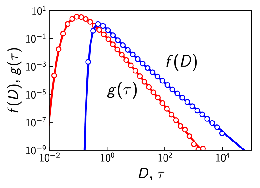
Figure 1: (color online) Distributions $g(\tau)$ (red) and $f(D)$ (blue). Lines: theoretical expressions,  (6) and  (7). Circles: histograms of the sample set of $\tau$ and $D$. $\tau_{*}=1$; $D_{*}=1$; $\alpha=3/2$; $\eta=1/2$.

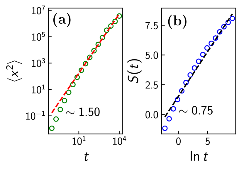
Figure 2: (color online) (a) MSD computed from the MC simulations (green circles) compared with the analytical prediction: $\langle x^{2}(t)\rangle\propto t^{\phi}$; $\phi=3/2=1.5$ (red dashed line). (b) Comparison of the DEA behavior computed from MC simulations (blue circles) with DEA computed from the analytically obtained PDF, Eq. (14) (dashed black line). $\delta=3/4=0.75$.

The DEA was computed using the histograms estimated from numerical MC simulations and from the numerical computation of the analytical expression (14). The comparison of the two different estimates is shown in Fig.  2(b). It is evident that the DEA computed from the analytical expression shows very good agreement with the theoretical scaling: $\delta=\phi/2=1-\eta/2=3/4$. On the contrary, in the DEA computed from MC simulations a net straight line in the graph $(\ln t,S(t))$ does not emerge clearly in the studied range, even if a rough agreement with the theoretical expectation is seen. This is probably due to statistical limitations of MC simulations, thus proving that estimation of scaling in such processes could be quite a delicate task when dealing with real experimental data.

In Fig. 3 we compare the coordinate PDFs computed from Eq. (14) with those evaluated from the MC simulations (being diffusion symmetrical, the PDFs are plotted in the range $x>0$).

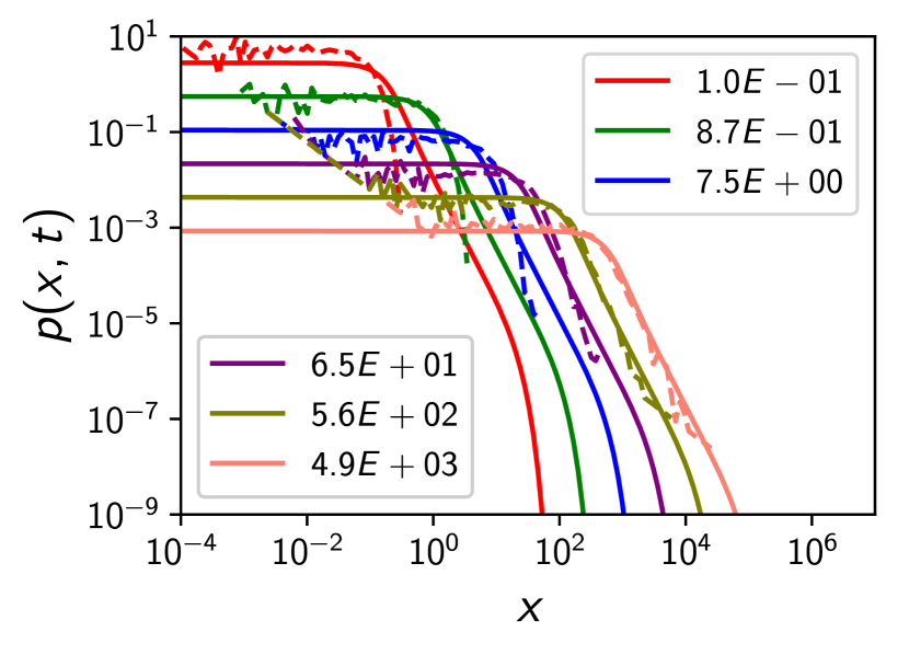
Figure 3: (color online) Comparison of the coordinate PDFs of the MC simulated motion (dashed lines) with that obtained from the analytical expression  (14) (straight lines) for different times.

The analytical expression clearly shows a well-defined power-law tail in a intermediate range of $|x|$: $p(x,t)\propto 1/|x|^{1+\alpha}$, followed by a rapid cut-off for large $|x|$. Regarding the space-time scaling $z=x/t^{\delta}$, in agreement with DEA, the analytical PDFs have an exact self-similarity index $\delta=3/4$. Conversely, the decay of PDFs derived from MC simulations is slightly more complicated, but the general behavior is compatible with the analytical one. Even the self-similarity space-time scaling roughly approximates the theoretical expectation $\delta=3/4$, but small deviations are evident, is agreement with the DEA displayed in Fig.  2(b) (blue circles).

2.4 Heterogeneous ensemble of Brownian particles and superstatistics

Superstatistics approach takes into account large-deviations of intensive quantities of systems in nonequilibrium stationary states [76, 77, 115] and it was motivated by some preliminary success obtained when fluctuations of parameters were considered [116, 117]. In general, superstatistics is successful to model: turbulent dispersion considering energy dissipation fluctuations [76, 118], renewal critical events in intermittent systems [119, 120], and for different distributions of the fluctuating intensive quantities different effective statistical mechanics can be derived [77], e.g., Tsallis statistics with $\chi^{2}$-distribution.

The main idea of superstatistics is that a Brownian test particle experiences fluctuations of some intensive parameters by moving from cell to cell [77]. Following this idea, the random value of the fluctuating parameter is generated at any change of cell. The main assumption behind this picture is that each cell is in equilibrium during the residence time of the particle: within the cell there are no fluctuations but a different value assigned to each cell. The local value of the fluctuating parameter changes in the various cells on a time scale that is much longer than the relaxation time that the single cells need to reach local equilibrium. This means that the fluctuating parameter follows a slow dynamics and then the integration over the fast variable is taken after the integration over the slow variable which is in opposition to what an adiabatic scheme requires [121]. This fact can be considered just an order of integration that does not affect the computation of the expected values but it is more deep when the entropy is considered [115, 121]. This inconsistency is solved by considering a dynamical equation also for the slow fluctuating quantity [121], an example of such dynamical equation was already considered in Ref. [118].

The HEBP approach is clearly based on a different picture, even if the superposition of Langevin equations may suggest some analogies. Here the superposition gives rise to anomalous diffusion because it reproduces the effects of the ensemble heterogeneity. In fact, in the present approach the fluctuations are not due to different values in different cells but to the population of density (mass divided by volume) of the ensemble. As a consequence of this, the present approach does not take into account slow and fast dynamics and then the issue concerning the order of integration does not arise.

2.5 Anomalous-to-normal transition

Here we briefly show the effect of limited statistics of $\tau$ on the diffusion scaling. Statistical limitation in the number of $\tau$ randomly drawn from $g(\tau)$ also results in the existence of a maximum relaxation time $\tau_{\rm max}$. Thus, the statistical limitation in the sample set of $\tau$ mimicks the existence of a $\tau_{\rm max}$ in real experimental systems. This is a reasonable assumption, also considering the relation of $\tau$ with mass and size of the particle (see previous Section 2.1), whose distributions are necessarily limited.

Figure 4: (color online) Histogram of a sample set of $\tau$ limited to $10000$ draws from $g(\tau)$. $\tau_{*}=1$.

In Fig. 4 we report the histogram for a sample set with $10000$ random draws from $g(\tau)$. The parameters are: $\eta=1/2$, $\langle\tau\rangle=1/2$. It can be seen that, for this limited statistics, $g(\tau)$ is well-reproduced up to a value of $\tau$ less than $10$, while for larger values there are fluctuations and, for $\tau$ greater than about $30-50$, also some apparent outliers are seen till a maximum value $\tau_{\rm max}=297.2$. The experimental/numerical mean relaxation time is $\langle\tau\rangle_{\rm exp}=0.52$.

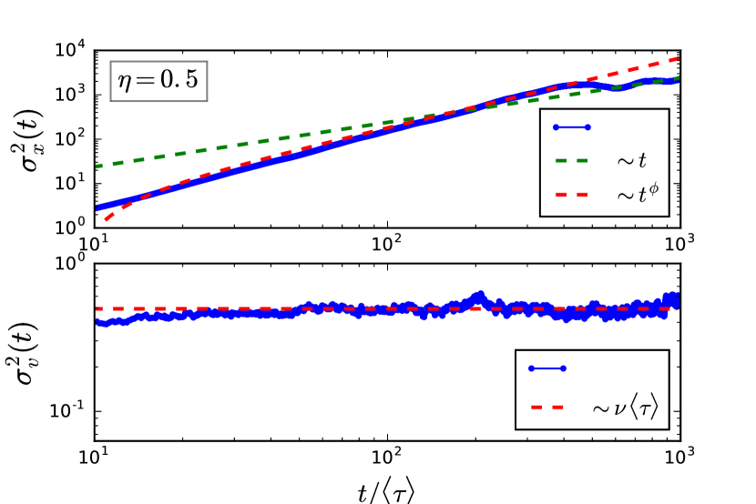
Figure 5: (color online) Numerical simulations of the heterogeneous ensemble of Brownian particles for the $\tau$ sample set of Fig. 4. Top panel: position MSD; bottom panel: velocity MSD.

The maximum relaxation time $\tau_{\rm max}$ can be considered a kind of time scale after which all trajectories reach the condition of a variance increasing linearly in time, even if with different multiplicative factors. As a consequence, we expect normal diffusion to occur in a very long time regime. This is confirmed in Fig. 5, where the anomalous diffusive scaling $\phi=2-\eta=3/2$ emerges in the approximate time interval $[15\langle\tau\rangle,450\langle\tau\rangle]$, after which there is a transition to a normal diffusion regime starting at $t\sim 600\langle\tau\rangle$. It is worth noting that, in general, the transition time scale does not depend only on $\tau_{\rm max}$, but also on the detailed statistics of the numerical histogram in the neighborhood of $\tau_{\rm max}$ itself. In particular, a situation where $\tau_{\rm max}$ is an outlier is quite different from a condition where $\tau$-set is, in some sense, dense near $\tau_{\rm max}$, which cannot then be considered an outlier.

In summary, we can argue that, depending on the experimental/numerical set of relaxation times $\tau$, our HEBP model reproduces a transition from anomalous to normal diffusion.

3 Comparison with Lévy walk models

LW is one of the best known models of anomalous diffusion with finite MSD and was firstly introduced by Shlesinger, Klafter and Wong in 1982 [59]. The number of papers devoted to LWs is very large (see, e.g., [114, 20, 57, 122, 123, 124, 125]) and a quite recent and complete review can be found in Zaburdaev et al., 2015 [61]. LWs have been applied to many phenomena, but surely the most promising and widespread applications are in the modeling of search strategies, such as bacteria foraging through run-and-tumble motion [126, 37, 61]. Unlike Lévy flights, where the particle is allowed to make large jumps in a whatever short time step (theoretically zero in the time-continuous limit), thus giving instantaneous infinite velocities and discontinuous paths, in LW models the particle moves with a finite speed. Such speed remains constant throughout a random duration time, also called Waiting Time (WT). After this WT, velocity randomly changes according to an assigned walking rule and it remains constant for another random WT. Thus, even if there are events with discontinuous acceleration, LWs have continuous velocity. When WT have a constant value, equivalent to a fixed time step, and velocity MSD is finite, LW reduces to a standard Random Walk with ballistic diffusion: $\langle x^{2}\rangle\sim t^{2}$. For WTs with finite mean, ballistic diffusion also occurs, but in the long-time limit (e.g., exponentially distributed WTs). Interestingly, the LW also displays strong anomalous diffusion, also known as multiscaling/multifractal diffusion [127, 128]. Multiscaling detection algorithms are usually based on the analysis of fractional moments:

$$\langle|x|^{q}\rangle=\int_{-\infty}^{\infty}\mathrm{d}x|x|^{q}p(x,t)=M_{q}\cdot t^{\lambda(q)}\ ,$$ (18)

where $\lambda(q)=qH(q)$, being $H(2)$ the well-known Hurst exponent or second-moment scaling. A complex system is multiscaling when $H$ changes with the moment order $q$ and the particular multiscaling features are defined by the behavior of the function $H(q)$. Conversely, a constant $H$, thus independent of $q$, is associated with monoscaling systems: $\langle|x|^{q}\rangle\sim t^{qH}$.

Here we consider two different LW models that differ for the velocity distribution. The first one is the most classical one with randomly alternating velocities, i.e., constant speed $|V_{{}_{\rm LW}}|$ and randomly changing direction according to a coin tossing prescription [59, 114, 61]. We limit here to the case $V_{{}_{\rm LW}}=\pm 1$. In the second one, we consider a continuous and symmetric random variable for the velocity [61]. In both LW models the velocity is constant throughout a WT of duration $\delta t_{i}=t_{i+1}-t_{i}$ and randomly changes in correspondence of the critical event $i+1$, whose occurrence time $t_{i+1}$ marks the passage from the WT $\delta t_{i}$ to the next WT $\delta t_{i+1}$. For the WT distribution, we consider the following PDF [56]:

$$\psi(\delta t)=\frac{\left(\mu-1\right)T^{\mu-1}}{\left(T+\delta t\right)^{\mu}},$$ (19)

where $\mu>1$ and $T$ is a reference time scale. The power-law tail emerges in the range $\delta t\gg T$. In the following we set $T=1$. The superdiffusive sub-ballistic behavior (the one we are interested in) is revealed when $2<\mu<3$. In the LW with alternating velocities, this regime is characterized by a central part of the PDF $p(x,t)$ that is well approximated by a symmetric Lévy stable density $L_{\alpha}^{0}$ with stability index $\alpha=1/(\mu-1)$ [114, 56]. At sufficiently large $|x|$, the PDF is abruptly truncated by ballistic peaks located at $x=\pm V_{{}_{\rm LW}}t$, which corresponds to the ballistic motion of paths whose first WT is longer than $t$.

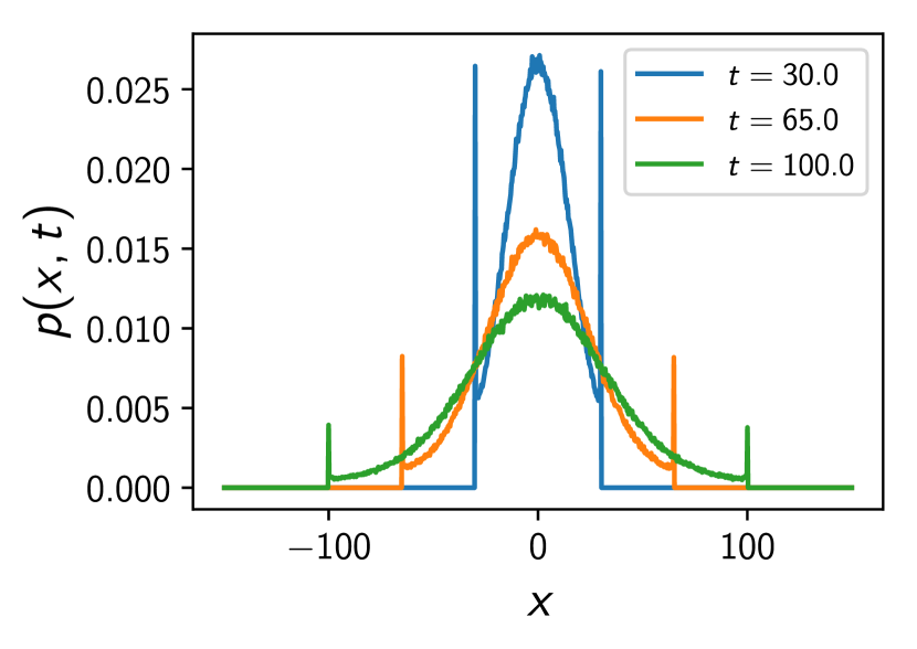
Figure 6: Lévy walk probability density functions: the central part looks like Lévy $\alpha$-stable law cut by ballistic fronts at $x=\pm V_{{}_{\rm LW}}t$

.

In Fig. 6 the PDFs at different times computed from a MC simulation of LW with alternating velocities are reported. The ballistic peaks truncating the PDFs are evident.

Similarly to HEBP, Eq.  (14), this LW model displays a power-law decay in a intermediate range of $|x|$ followed by an abrupt cut-off, thus resulting in the finiteness of moments and, in particular, of the MSD: $\langle x^{2}\rangle\propto t^{4-\mu}$ [114, 61]. For the LW with randomly alternating velocities and WT-PDF given by  (19) , the fractional moments are given by [61]:

$$\lambda(q)=\left\{\begin{array}[]{l}q/(\mu-1)\ ;\quad\quad\ \ q\leq\mu-1\ ;\\ \\ q-(\mu-2)\ ;\qquad q>\mu-1\ .\end{array}\right.$$ (20)

It is then easily seen from this formula that the LW with randomly alternating velocities obeys a biscaling law, with a given scaling for low-order moments and another one for high-order moments.

In the following we compare four different cases: two LW models (with alternating and continuous velocities, respectively) and our HEBP model for two different sets of parameters chosen to fit the LW models. In particular:

• Lévy walk with randomly alternating velocity rule. WT-PDF given by Eq.  (19) with $\mu=5/2$. Coin tossing prescription for the change of direction. We set $V_{{}_{\rm LW}}=\pm 1$, so that $\langle v^{2}\rangle_{\rm eq}=\langle v^{2}_{{}_{\rm LW}}\rangle=1$;

• HEBP analytical model, Eq. (14), with parameters: $\alpha=3/2$, $\eta=1/2$, $\langle v^{2}\rangle_{\rm eq}=\langle\tau\rangle\langle D\rangle=1$. It results: $\langle\tau\rangle=1/2$, $\langle D\rangle=2$, $\phi=2-\eta=3/2$ and $D_{\mathrm{max}}=40.1$ (numerically calculated from Eq.  (15));

• Lévy walk with random continuous velocity. WT-PDF given by Eq.  (19) with $\mu=5/2$. The velocity PDF is symmetric and evaluated from the stationary state of MC simulations carried out for the HEBP, Eq.  (14). MC simulation parameters are the same as in the next case (iv). The random generation of velocities was performed with the inverse transform sampling method;

• HEBP analytical model, Eq. (14), with parameters: $\alpha=3/2$, $\eta=1/2$, $\langle v^{2}\rangle_{\rm eq}=\langle\tau\rangle\langle D\rangle=8.127$. It results: $\langle\tau\rangle=1/2$, $\phi=2-\eta=3/2$, $\langle D\rangle=16.254$ and $D_{\mathrm{max}}=1.43\cdot 10^{5}$ (numerically calculated from Eq.  (15));

The PDFs $p(x,t)$ of the HEBP, cases (ii) and (iv), are obtained, for different times, by means of numerical evaluation of Eq.  (14). Then, DEA $S(t)$ and MSD $\langle x^{2}(t)\rangle$ are computed by the calculated PDFs. Conversely, the paths of LW models (i) and (iii) are computed by means of MC stochastic simulations and, then, PDFs, DEA and MSDs are evaluated by statistical analysis of the sample paths.

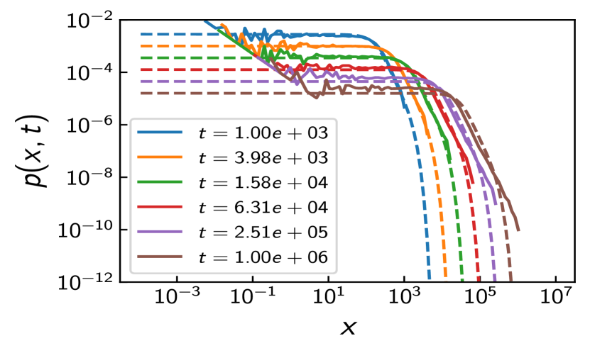
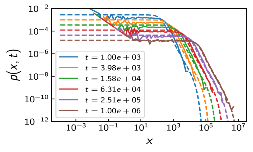
Figure 7: Comparison of PDFs $p(x,t)$ for the four model cases (i-iv): Top panel: LW model (i) with randomly alternating velocities (solid lines) fitted by HEBP, case (ii) (dashed lines); Bottom panel: LW model (iii) with continuous random velocities (solid lines) fitted by HEBP, case (iv) (dashed lines).

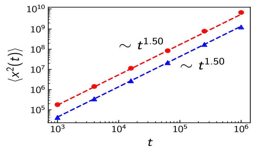
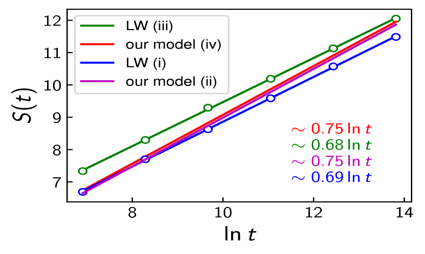
Figure 8: Comparison of MSD $\langle x^{2}\rangle(t)$ and DEA $S(t)$, Eq. (17)), for the four model cases (i-iv): Top panel: LW model (i) with randomly alternating velocities (blue triangles); HEBP, case (ii) (dashed blue line); LW model (iii) with random continuous velocities (red circles); HEBP, case (iv) (dashed red line); Bottom panel: LW model (i) with randomly alternating velocity (blue dots and line); HEBP, case (ii) (purple line); LW model (iii) with random continuous velocity (green dots and line); HEBP, case (iv) (red line).

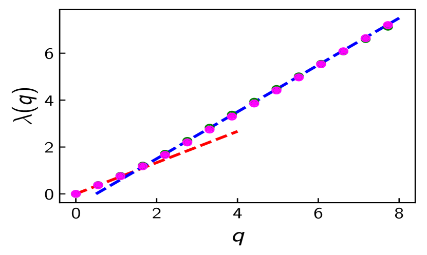
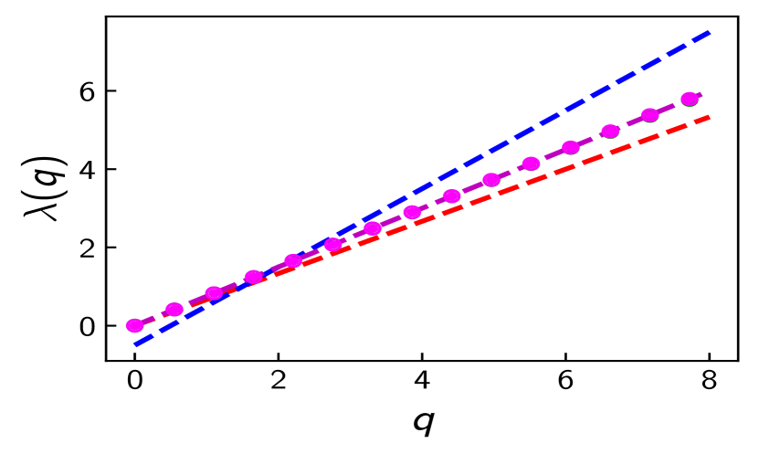
Figure 9: Top panel: fractional moments, (Eq. (18)), of LW models (i) and (iii) (purple and green points, respectively – almost coincide), dashed lines are analytical asymptotes given by Eq.  (20); Bottom panel: fractional moments of HEBP, cases (ii) and (iv) (purple and green points, respectively – almost coincide), dashed lines are the same analytical asymptotes as in Top panel.

The results are gathered in Figs.  7, 8 and  9. In Fig.  7 the comparisons of position PDFs $p(x,t)$ for different times are shown: LW model (i) fitted by HEBP, case (ii) (top panel) and LW model (iii) fitted by HEBP, case (iv). It is evident that the two LW models (alternating/continuous velocities) have very similar behaviors and that, for both models, it is always possible to find a parameter set for the HEBP to be comparable with LW models. In particular, HEBP well reproduces the power-law decay in the intermediate range, while for $x$ greater than the ballistic peaks of LW models an exponential cut-off emerges in the PDFs of HEBP. However, the space-time scaling $\delta$ is clearly different for the two models, as it is clear from the slight shifts between solid and dashed lines in both panels. Then, for fixed set of parameters, the quality of the fit is not the same for all PDF times. In particular, in the top panel (models (i) and (ii)) the best fit is made at time $t=10^{3}$, so that the less accurate agreement is at the longest time $t=10^{6}$. On the contrary, in the bottom panel the best fit is made at $t=10^{6}$ and, consequently, the worst agreement is at the first displayed time $t=10^{3}$.

In Fig.  8 we report the MSD $\langle x^{2}\rangle$ (Top panel) and the DEA $S(t)$ (Bottom panel) for the four model cases. Numerical simulations and calculations of all models (i-iv) (LW models and HEBP) reproduce the expected power-law dependence $\langle x^{2}\rangle\sim t^{3/2}$ with a very good agreement. The DEA $S(t)$ shows the net differences of the self-similarity index $\delta$ among LW and HEBP, thus making it more evident the different space-time scaling seen in Fig.  7. The numerical scaling is also in agreement with theoretical values: $\delta=1/(\mu-1)=2/3\simeq 0.67$ for LWs and $\delta=1-\eta/2=3/4$ for HEBP.

Finally, in order to explore the multiscaling character of the models, Fig.  9 show the results for the evaluation of fractional moments. In top panel the fractional moments of LW model (i) and (iii) are compared, while bottom panel compares HEBP, cases (i) and (iv). The LW models (i) and (iii) have exactly the same behavior for $\lambda(q)$, thus in agreement with the expected multiscaling and, in particular, the biscaling law of Eq.  (20). The behavior of our numerical simulations of HEBP, cases (ii) and (iv), is also found to be very similar to each other and in agreement with theoretical predictions, that is, it shows a well-defined monoscaling. The space-time scaling is the same for both parameter sets, as it depends only on $\eta$, being $\langle X^{q}\rangle\sim t^{\lambda(q)}=t^{qH(q)}$ with:

$$H(q)=\phi/2=1-\eta/2,$$ (21)

and, for HEBP, this is also equal to the self-similarity index: $\delta=H(q)=\phi/2$ (see Eq.  (12)).

4 Discussion and concluding remarks

We here introduced and discussed a model based on the idea of a standard friction-diffusion process in a strongly heterogeneous condition with inverse power-law distributions of parameter’s populations (Eqs.  (6) and  (7)). We considered the Langevin equation for an Ornstein–Uhlenbeck process with randomly distributed relaxation/correlation times $\tau$ and diffusivities $D$. The model with random $\tau$ population and constant diffusivity gives a Gaussian process with long-range correlation and anomalous diffusion scaling. The moments $\langle|x|^{q}\rangle$ are finite, as well as the energy $\langle v^{2}\rangle_{\rm eq}$. However, anomalous transport often displays power-law decays in the position PDF $p(x,t)$ that cannot be reproduced by Gaussian processes, even if long-range. In order to extend this model to non-Gaussian PDFs with power-law tails, a random $D$ population is needed. This is obtained by means of the distribution $f(D)$ given in Eq.  (7). However, this distribution has an infinite mean and determine infinite moments for the velocity PDF and, thus, infinite energy. This is an unphysical condition, which also prevents to get a fluctuation-dissipation relation. For this reason we adopted a more realistic assumption by imposing a cut-off maximum value $D_{\rm max}$ for the diffusivity population, from which Eq.  (14) follows.

We proved that, similarly to LWs, our proposed HEBP model can take into account intermediate power-law decays in the PDF. Unlike LWs, where power-law is truncated by the ballistic peaks due to the underlying WT statistics, in HEBP the power-law is truncated by an exponential cut-off in the regime of large $x$. In experimental data, this is often associated with lack of statistics or presence of noise [129, 57, 58], but it is also recognized to be reminiscent of heterogeneous media [71].

In summary, we derived a model in a physical framework involving heterogeneity and, then, a population of parameters characterized by given inverse power-law distributions. Our model follows from a superposition of standard Gaussian processes with stationary and independent increments. This model therefore has the following properties:

• long-range correlations $R(t)\sim 1/t^{\eta}$ and anomalous superdiffusive scaling in the variance: $\langle x^{2}\rangle\sim t^{\phi}$ ($\phi=2-\eta$; $1\leq\phi<2$);

• finite moments $\langle|x|^{q}\rangle$, finite energy $\langle v^{2}\rangle_{\rm eq}$ and a fluctuation-dissipation relation:
  $\langle v^{2}\rangle_{\rm eq}=\langle\tau\rangle\langle D\rangle$;

• both an intermediate range with power-law decay $1/|x|^{1+\alpha}$ and an asymptotic range with exponential cut-off in the PDF $p(x,t)$;

• space-time monoscaling behavior: $x\sim t^{\delta}$
  ($\delta=\phi/2$);

• $\alpha$ and $\delta$ are independent scaling parameters;

• a transition from anomalous (intermediate time regime) to normal diffusion (long time regime).

This last point implies that the (mono-)scaling index $\delta$ is a function of time, being $\delta(t)\neq 1/2$ for $t$ much less than the maximum relaxation time $\tau_{\rm max}$, and $\delta(t)=1/2$ for $t\gg\tau_{\rm max}$.

Properties (1-3) are similar to those displayed by LW models, apart from the exponential cut-off of HEBP, which could be difficult to distinguish from the cut-off in the LW-PDF when dealing with experimental data.

On the contrary, property (4) is not satisfied by LWs, which obey the biscaling law  (20), distinctly different from the monoscaling behavior of HEBP. Also the crucial property (5) is not seen in LWs.

Further, Lévy Walks do not reproduce the right space-time scaling $\delta$ of HEBP neither in the PDF’s central part, which is that part of the PDF more similar to a pure Lévy stable density. In fact, in our HEBP model the space-time scaling $\delta$ and the power-law decay of the probability distribution $\alpha$ are independent parameters, while they are not in LWs. LW is only driven by the parameter $\mu$ associated with the underlying trapping mechanism described by Eq.  (19). The additional assumption of jumps coupled with WTs triggers the emergence of anomalous superdiffusion, thus directly affecting the space-time self-similarity index $\delta_{{}_{\rm LW}}$.

Thus, when the LW-PDF is characterized by the decay: $p(x,t)\sim 1/|x|^{\mu}$, the scaling $\delta_{{}_{\rm LW}}$ is constrained, by the jump-WT coupling, to obey the relationship [114, 61]:

$$\delta_{{}_{\rm LW}}=\frac{1}{\mu-1}=\frac{1}{\alpha_{{}_{\rm LW}}}\ .$$ (22)

where $\alpha_{{}_{\rm LW}}=\mu-1$ represents the Lévy stability index. As known, this is well-established in the intermediate range where the LW-PDF is more similar to a pure Lévy stable density $L^{0}_{\alpha_{{}_{\rm LW}}}$. It is important to notice that the above relationship among $\delta$ and $\alpha$ can be also satisfied by our HEBP model for particular parameter choices, i.e., given the experimental $\alpha$, for $\eta=2-2/\alpha$.

Another important aspect worthy of discussion is the physical basis of the considered models. HEBP models directly follow from an heterogeneity assumption applied to a standard Gaussian process, whether the origin of heterogeneity is (in the medium or in the particle parameters). Thus, HEBP models, which are based on the same idea of the ggBM [89, 93], are derived from a physical background directly involving the idea of a complex heterogeneity and indeed we expect HEBP models to be more suitable to heterogeneous transport phenomena. Conversely, LWs should better fit phenomena where trapping plays a fundamental role.

As already said, many authors have recently been focusing on position transport models with heterogeneous diffusivities, e.g., DDMs [79, 80, 81, 71, 72]. In some sense, HEBP models belong to the class of transport models with random diffusivity, i.e., HDMs. However, unlike other ones, the HEBP model here discussed explicitly describes the velocity dynamics, thus including the often neglected but crucial role of viscous relaxation time $\tau$. More precisely, we here refer to the relaxation time of the velocity, a physical parameter whose relationship with medium/fluid properties is well-established. As seen above, the role of heterogeneity in the relaxation time $\tau$ is taken into account and modeled through a population with inverse power-law distribution $g(\tau)$. Another important aspect is that the here proposed HEBP model is derived from a standard friction-diffusion process having finite energy and satisfies a fluctuation-dissipation theorem.

From the above discussion, we can finally suggest a possible statistical recipe to distinguish the best modeling approach among LWs and HEBP models starting from a set of experimental transport data. This is of great interest when the underlying mechanism, heterogeneity or trapping, driving anomalous diffusion is not yet clear. If the experimental PDF displays a power-law decay, it is possible to apply a best fit procedure to get $p(x,t)\sim 1/|x|^{1+\alpha_{{}_{\rm exp}}}$ for some $\alpha_{{}_{\rm exp}}<2$, where ’exp’ stands for experimental. Then, fractional moments and the function $\lambda(q)=qH(q)$ can be computed. DEA can be applied to compute the self-similarity index and let us assume that a well-defined $\delta$ exists. Then, we have the indices $\alpha_{{}_{\rm exp}}$, $\delta$ and $\lambda(q)$. If the data are monoscaling, then HEBP could be a good candidate and we have two parameters to independently fit the PDF scaling ($\alpha$) and the moment scaling ($H(q)=\phi/2=$ constant). The exponential cut-off could be another clue towards HEBP [71], but actually an exponential cut-off is usually seen in the tail of experimental PDFs due to lack of statistics and/or presence of instrumental/environmental noise. If data are multiscaling, then there are two possibilities: (i) biscaling law  (20) is satisfied for some $\mu=1+\alpha_{{}_{\rm exp}}$ and LW modeling approach is the most reasonable one; (ii) other multiscaling laws, biscaling or not, emerge and neither LW nor HEBP cannot be applied.

Appendix A Numerical algorithms

In the following we shortly describe the algorithms used for numerical evaluations and stochastic simulations.

• Langevin equation  (4) for $(x,v)$ is numerically integrated by using a Euler scheme.

• The random drawings from the PDF $f(D)$ are carried out by means of the Chambers–Mallows–Stuck algorithm for the simulation of extremal Lévy densities $L_{\alpha}^{-\alpha}$ in the interval $0<\alpha<1$ [130, 131, 96].

• To get random drawings from $g(\tau)$, we first obtained a numerical PDF by applying the Chambers–Mallows–Stuck algorithm to the Lévy extremal density $L_{\eta}^{-\eta}$ with very high statistics, and then we computed the numerical histogram and the function $g(\tau)$ using Eq.  (6). This numerical PDF $g(\tau)$ is then used to draw number by the cumulative function method [see also details in Ref. [100]].

• The HEBP-PDF with maximum diffusivity $D_{\rm max}$, given by Eq.  (14), is evaluated by the numerical calculation of the integral. This is done by applying a composite trapezoidal rule with sufficiently small step $\delta D$.

• In the stochastic simulations we used $\alpha=3/2$, $\eta=1/2$ (so that the MSD is $\langle x^{2}\rangle\propto t^{3/2}$), initial conditions $x_{i,0}=0$ and $v_{i,0}=0$. $10^{4}$ trajectories were simulated, being each trajectory obtained as an average over a set of $N=9600$ couples $(\tau,D)$ drawn from $g(\tau)$ and $f(D)$ (for a total of $9.6\cdot 10^{7}$ drawn couples $(\tau,D)$). The programs for the simulations were written in the c++ language (Debian gcc 4.9) and Python 2.7.

A final observation is in order. A single trajectory of the HEBP can be interpreted as resulting from the superposed effects of $D$ and, especially, $\tau$ populations. We applied this approach in performing the numerical simulations. In particular, for a fixed diffusivity value $D$, the HEBP model becomes a Gaussian process with long-range time correlation and variance given by Eqs.  (8) and  (9), respectively. This is a consequence of the Central Limit Theorem, as the process results from a linear superposition of independent Gaussian processes.
Alternatively, the model can be interpreted as a set of different particles whose motion $(x(t),v(t))$ is driven by heterogeneous parameters $(\tau,D)$. Thus, the average motion can be derived as an average over this ensemble of trajectories.
To the goal of stochastic simulations the two approaches are mathematically equivalent. The two physical interpretations of the trajectories are different, but the possibility of guessing the correct interpretation depend on the possibility of observing a sufficiently large number of single trajectories with high precision, so that both single particle and ensemble statistics can be computed (similarly to the direct evaluation of ergodic condition).

Appendix B From HEBPs to RSGPs

The dynamical equations of an ensemble of particles moving in a viscous fluid and having homogeneous parameters $\tau$ and $D$ are:

$$\frac{dx}{dt}=v\ ,$$

$$\frac{dv}{dt}=-\frac{1}{\tau}v(t)+\sqrt{2D}\,\xi(t)\ .$$

The Langevin equation for $v(t)$ is formally the same as Eq.  (4), but without the index $i$. Let us assume that some randomness is assumed for the the diffusivity $D$ and let us write the process $(x(t),v(t))$ as:

$$x(t)=\sqrt{2D}\,x_{G}(t)\ ;\quad v(t)=\sqrt{2D}\,v_{G}(t)\ .$$

by substituting in the previous equations, we get a Langevin equation with unitary noise intensity:

$$\frac{dx_{G}}{dt}=v_{G}\ ,$$

(23)

$$\frac{dv_{G}}{dt}=-\frac{1}{\tau}v_{G}(t)+\xi(t)\ .$$

It is well known that the solution for the PDF $p(x_{G},v_{G},t)$ and, consequently, for the marginal PDFs of $x_{G}$ and $v_{G}$, are Gaussian. Thus, the process $(x_{G}(t),v_{G}(t))$ is a Gaussian process.

This proves that the process $(x(t),v(t))$ derived from the randomization of the velocity diffusivity $D$ is equivalent to a RSGP with random amplitude given by $\sqrt{2D}$, while the Gaussian process is “generated” by a Langevin equation with unitary noise intensity.

When a population of relaxation times $\tau$ with a complex PDF $g(\tau)$ is considered, the randomized Langevin equation  (23) still gives a Gaussian process but, depending on $g(\tau)$, the global correlation function can be non-exponential and, thus, diffusion can be non-standard. In particular, when $g(\tau)$ is given by Eq.  (6), the correlation function is long-range (i.e., slow power-law decaying) and anomalous diffusion emerges.

References

References

- [1] Rice S A 1985 Diffusion-Limited Reactions (New York: Elsevier) ISBN 9780080868196
- [2] Dorsaz N, De Michele C, Piazza F, De Los Rios P and Foffi G 2010 Phys. Rev. Lett. 105(12) 120601
- [3] Kaplan H, Dinar N, Lacser A and Alexander Y (eds) 1993 Transport and Diffusion in Turbulent Fields: Modeling and Measurement Techniques 1st ed (Netherlands: Springer) ISBN 978-94-010-5220-7
- [4] Paradisi P, Cesari R, Mainardi F and Tampieri F 2001 Physica A 293 130–142
- [5] Paradisi P, Cesari R, Mainardi F, Maurizi A and Tampieri F 2001 Phys. Chem. Earth 26 275–279
- [6] Paradisi P, Cesari R, Donateo A, Contini D and Allegrini P 2012 Nonlinear Proc. Geoph. 19 113–126 p. Paradisi et al., Corrigendum, Nonlin. Processes Geophys. 19, 685 (2012)
- [7] Cheng X, Hu F and Zeng Q 2014 Chin. Sci. Bull. 59 4890–4898 ISSN 1861-9541
- [8] Goulart A, Lazo M, Suarez J and Moreira D A 2017 Physica A 477 9–19
- [9] Ingenhousz J 1784 Vermischte schrifen physisch medicinischen inhalts vol 2 (Vienna: Wappler)
- [10] Bywater J 1828, first published in 1819 Physiological Fragments: To Which are Added Supplementary Observations, to Show that Vital Energies are of the Same Nature, and Both Derived from Solar Light (London: R. Hunter)
- [11] Brown R 1828 Phil. Mag. 4 161–173
- [12] Brown R 1829 Phil. Mag. 6 161–166
- [13] Derek Abbott D, Davis B R, Phillips N J and Eshraghian K 1996 IEEE Trans. Educ. 39 1–13
- [14] Perrin J 1908 Compt. Rend. 146 967
- [15] Perrin J 1909 Ann. Chim. Phys. 18 5
- [16] Metzler R and Klafter J 2000 Phys. Rep. 339 1–77
- [17] Paradisi P, Kaniadakis G and Scarfone A M 2015 Chaos Soliton Fract 81 407–11
- [18] Paradisi P, Kaniadakis G and Scarfone A M (eds) 2015 The emergence of self-organization in complex systems (Amsterdam: Elsevier) Special Issue - Chaos, Soliton Fract, Vol. 81(B), Pages 407-588
- [19] Metzler R and Klafter J 2004 J. Phys. A: Math. Theor. 37 R161–R208
- [20] Klages R, Radons G and Sokolov I M (eds) 2008 Anomalous Transport: Foundations and Applications (Weinheim: Wiley-VCH)
- [21] Richardson L 1926 Proc. R. Soc. A 110 709
- [22] Montroll E 1964 Proc. Symp. Appl. Math., Am. Math. Soc. 16 193–220
- [23] Montroll E W and Weiss G H 1965 J. Math. Phys. 6 167–181
- [24] Scher H and Montroll E W 1975 Phys. Rev. B 12(6) 2455–2477
- [25] Solomon T, Weeks E and Swinney H 1993 Phys. Rev. Lett. 71 3975–3978
- [26] Kraichnan R 1994 Phys. Rev. Lett. 72 1016–1019
- [27] Clausen S, Helgesen G and Skjeltorp A 1997 Physica A 238 198–210
- [28] Venkataramani S, Antonsen T and Ott E 1998 Phys. D 112 412–440
- [29] Periasamy N and Verkman A 1998 Biophys. J. 75 557–567
- [30] Del-Castillo-Negrete D, Carreras B and Lynch V 2004 Phys. Plasmas 11 3854–3864
- [31] Florian Furstenberg F, Dolgushev M and Blumen A 2015 Chaos Soliton Fract 81 527 – 533 ISSN 0960-0779
- [32] Tolić-Nørrelykke I M, Munteanu E L, Thon G, Odderhede L and Berg-Sørensen K 2004 Phys. Rev. Lett. 93 078102
- [33] Golding I and Cox E C 2006 Phys. Rev. Lett. 96 098102
- [34] Gal N and Weihs D 2010 Phys. Rev. E 81 020903(R)
- [35] Barkai E, Garini Y and Metzler R 2012 Phys. Today 65 29
- [36] Manzo C and Garcia-Parajo M 2015 Rep. Progr. Phys. 78 124601
- [37] Ariel G, Rabani A, Benisty S, Partridge J D, Harshey R M and Be’Er A 2015 Nat. Comm. 6
- [38] He W, Song H, Su Y, Geng L, Ackerson B, Peng H and Tong P 2016 Nat. Comm. 7
- [39] Jeon J H, Tejedor V, Burov S, Barkai E, Selhuber-Unkel C, Berg-Sørensen K, Oddershede L and Metzler R 2011 Phys. Rev. Lett. 106 048103
- [40] Hofling F and Franosch T 2013 Rep. Prog. Phys. 76 046602
- [41] Manzo C, Torreno-Pina J A, Massignan P, Lapeyre G J, Lewenstein M and Garcia–Parajo M F 2015 Phys. Rev. X 5 011021
- [42] Molina-García D, Pham T M, Paradisi P, Manzo C and Pagnini G 2016 Phys. Rev. E 94 052147
- [43] Reverey J, Jeon J H, Bao H, Leippe M, Metzler R and Selhuber-Unkel C 2015 Sci. Rep. 5 11690
- [44] Metzler R, Jeon J H and Cherstvy A 2016 Biochim. Biophys. Acta 1858 2451–2467
- [45] Jeon J H, Javanainen M, Martinez-Seara H, Metzler R and Vattulainen I 2016 Phys. Rev. X 6
- [46] JA D and AS V 2008 Annu. Rev. Biophys. 37 247–263
- [47] Nawrocki G, Wang P H, Yu I, Sugita Y and Feig M 2017 J. Phys. Chem. B 121 11072–11084
- [48] Kuruma Y, Stano P, Ueda T and Luisi P 2009 BBA–Biomembranes 1788 567–574
- [49] Luisi P, Allegretti M, de Souza T, Steiniger F, Fahr A and Stano P 2010 ChemBioChem 11 1989–1992
- [50] Paradisi P, Allegrini P and Chiarugi D 2015 BMC Syst. Biol. 9
- [51] Weiss G and Rubin R 1983 Adv. Chem. Phys. 52 363–505
- [52] Bouchaud J P and Georges A 1990 Phys. Rep. 195 127–293
- [53] and J P B 1992 J. Phys. I France 2 1705–1713
- [54] Bianco S, Grigolini P and Paradisi P 2007 Chem. Phys. Lett. 438 336–340
- [55] Paradisi P, Cesari R, Contini D, Donateo A and Palatella L 2009 Eur. Phys. J.-Spec. Top. 174 207–218
- [56] Paradisi P, Cesari R, Donateo A, Contini D and Allegrini P 2012 Rep. Math. Phys. 70 205–220
- [57] Paradisi P and Allegrini P 2015 Chaos Soliton Fract 81 451–62
- [58] Paradisi P and Allegrini P 2017 Intermittency-driven complexity in signal processing Complexity and Nonlinearity in Cardiovascular Signals ed Barbieri R, Scilingo E P and Valenza G (Cham: Springer) pp 161–196 ISBN 978-3-319-58708-0
- [59] Shlesinger M F, Klafter J and Wong Y M 1982 J. Stat. Phys. 27 499–512
- [60] Shlesinger M F, Klafter J and West B J 1986 Physica A 140 212–218
- [61] Zaburdaev V, Denisov S and Klafter J 2015 Rev. Mod. Phys. 87 483–530
- [62] Burov S, Jeon J H, Metzler R and Barkai E 2011 Phys. Chem. Chem. Phys. 13 1800–1812
- [63] de Jager M, Weissing F J, Herman P M J, Nolet B A and van de Koppel J 2011 Science 332 1551–1553
- [64] Mandelbrot B B and Van Ness J W 1968 SIAM Rev. 10 422–437
- [65] Biagini F, Hu Y, Øksendal B and Zhang T 2008 Stochastic Calculus for Fractional Brownian Motion and Applications (Springer) ISBN 978-1-85233-996-8
- [66] Heppe B M O 1998 J. Fluid Mech. 357 167–198
- [67] Goychuk I 2013 Adv. Chem. Phys. 150 187–253
- [68] Goychuk I, Kharchenko V and Metzler R 2014 PLoS ONE 9
- [69] Stella L, Lorenz C D and Kantorovich L 2014 Phys. Rev. B 89(13) 134303
- [70] Massignan P, Manzo C, Torreno-Pina J, García-Parajo M, Lewenstein M and Lapeyre Jr G 2014 Phys. Rev. Lett. 112 150603
- [71] Lanoiselée Y and Grebenkov D 2018 J. Phys. A: Math. Theor. 51
- [72] Sposini V, Chechkin A V, Seno F, Pagnini G and Metzler R 2018 New J. Phys. 20 043044
- [73] Cherstvy A, Chechkin A and Metzler R 2013 New J. Phys. 15 083039
- [74] Jeon J H, Chechkin A V and Metzler R 2014 Phys. Chem. Chem. Phys. 16 15811–15817
- [75] Cherstvy A and Metzler R 2016 Phys. Chem. Chem. Phys. 18 23840
- [76] Beck C 2001 Phys. Rev. Lett. 87(18) 180601
- [77] Beck C and Cohen E 2003 Physica A 322 267–275
- [78] Van Der Straeten E and Beck C 2009 Phys. Rev. E 80
- [79] Chubynsky M and Slater G 2014 Phys. Rev. Lett. 113 098302
- [80] Chechkin A V, Seno F, Metzler R and Sokolov I M 2017 Phys. Rev. X 7(2) 021002
- [81] Jain R and Sebastian K 2017 J. Chem. Sci. 129 929–937
- [82] Schneider W 1990 Grey noise Stochastic processes, physics and geometry ed et al S A (Teaneck, NJ: World Sci. Publ.) p 676–681
- [83] Schneider W 1992 Grey noise Ideas and methods in mathematical analysis, stochastics, and applications (Oslo, 1988) (Cambridge: Cambridge Univ. Press) p 261–282
- [84] Mainardi F, Mura A and Pagnini G 2010 Int. J. Differ. Equations 2010 104505
- [85] Pagnini G 2013 Fract. Calc. Appl. Anal. 16 436–453
- [86] Gorenflo R, Mainardi F, Moretti D and Paradisi P 2002 Nonlin. Dynam. 29 129–143
- [87] Paradisi P 2015 Comm. Appl. Ind. Math. 6
- [88] Sandev T, Metzler R and Chechkin A 2018 Fract. Calc. Appl. Anal. 21 10–28
- [89] Mura A 2011 Non-Markovian Stochastic Processes and Their Applications: From Anomalous Diffusion to Time Series Analysis (Lambert Academic Publishing) Ph.D. Thesis, Physics Department, University of Bologna, 2008
- [90] Mura A, Taqqu M S and Mainardi F 2008 Physica A 387 5033–5064
- [91] Mura A and Pagnini G 2008 J. Phys. A: Math. Theor. 41 285003
- [92] Mura A and Mainardi F 2009 Integr. Transf. Spec. F. 20 185–198
- [93] Pagnini G, Mura A and Mainardi F 2012 Int. J. Stoch. Anal. 2012 427383
- [94] Pagnini G, Mura A and Mainardi F 2013 Phil. Trans. R. Soc. A 371 20120154
- [95] Pagnini G 2012 Fract. Calc. Appl. Anal. 15 117–127
- [96] Pagnini G and Paradisi P 2016 Fract. Calc. Appl. Anal. 19 408–440
- [97] Gorenflo R, Mainardi F, Moretti D, Pagnini G and Paradisi P 2002 Chem. Phys. 284 521–541
- [98] Gorenflo R, Mainardi F, Moretti D, Pagnini G and Paradisi P 2002 Physica A 305 106–112
- [99] Mainardi F, Luchko Y and Pagnini G 2001 Fract. Calc. Appl. Anal. 4 153–192
- [100] Vitali S, Sposini V, Sliusarenko O, Paradisi P, Castellani G and Pagnini G 2018 arXiv:1806.11508
- [101] D′Ovidio M, Vitali S, Sposini V, Sliusarenko O, Paradisi P, Castellani G and Pagnini G 2018 arXiv:1806.11351
- [102] Gheorghiu S and Coppens M O 2004 Proc. Natl. Acad. Sci. USA 101 15852–15856
- [103] Barenblatt G I 1979 Similarity, Self–Similarity, and Intermediate Asymptotics (New York: Consultants Bureau)
- [104] Bodrova A S, Chechkin A V, Cherstvy A G, Safdari H, Sokolov I M and Metzler R 2016 Sci. Rep. 6 30520
- [105] Sancho J M, Lacasta A M, Lindenberg K, Sokolov I M and Romero A H 2004 Phys. Rev. Lett. 92 250601
- [106] Rozenfeld R, Łuczka J and Talkner P 1998 Phys. Lett. A 249 409–414
- [107] Łuczka J, Talkner P and Hänggi P 2000 Physica A 278 18–31
- [108] Łuczka J and Zaborek B 2004 Acta Phys. Pol. B 35 2151–2164
- [109] Ausloos M and Lambiotte R 2006 Phys. Rev. E 73 011105
- [110] Pagnini G 2014 Physica A 409 29–34 ISSN 03784371
- [111] Gnedenko B V and Kolmogorov A N 1954 Limit distributions for sums of independent random variables (Cambridge, MA: Addison-Wesley,)
- [112] Feller W 1971 An Introduction to Probability Theory and its Applications 2nd ed vol 2 (New York: Wiley)
- [113] Grigolini P, Palatella L and Raffaelli G 2001 Fractals 09 439–449
- [114] Allegrini P, Bellazzini J, Bramanti G, Ignaccolo M, Grigolini P and Yang J 2002 Phys. Rev. E 66
- [115] Abe S, Beck C and Cohen E G D 2007 Phys. Rev. E 76 031102
- [116] Wilk G and Włodarczyk Z 2000 Phys. Rev. Lett. 84 2770–2773
- [117] Beck C 2002 Europhys. Lett. 57 329–333
- [118] Reynolds A M 2003 Phys. Rev. Lett. 91 084503
- [119] Paradisi P, Cesari R and Grigolini P 2009 Cent. Eur. J. Phys. 7 421–431
- [120] Akin O, Paradisi P and Grigolini P 2009 J. Stat. Mech.: Theory Exp. P01013
- [121] Abe S 2014 Found. Phys. 44 175–182
- [122] Magdziarz M and Zorawik T 2016 Phys. Rev. E 94 022130
- [123] Taylor-King J P, Klages R, Fedotov S and Van Gorder R A 2016 Phys. Rev. E 94 012104
- [124] Dybiec B, Gudowska-Nowak E, Barkai E and Dubkov A A 2017 Phys. Rev. E 95(5) 052102
- [125] Aghion E, Kessler D and Barkai E 2018 Eur. Phys J. B 91
- [126] Viswanathan G M, da Luz M G, Raposo E and Stanley E 2011 The Physics of Foraging: An Introduction to Random Searches and Biological Encounters (Cambridge: Cambridge University Press) ISBN 9781107006799
- [127] Ott E 2002 Chaos in Dynamical Systems 2nd ed (Cambridge: Cambridge University Press) ISBN 0521432154
- [128] Kantelhardt J, Zschiegner S, Koscielny-Bunde E, Havlin S, Bunde A and Stanley H 2002 Physica A 316 87–114
- [129] Allegrini P, Menicucci D, Bedini R, Gemignani A and Paradisi P 2010 Phys. Rev. E 82(1) 015103
- [130] Chambers J M, Mallows C L and Stuck B W 1976 J. Amer. Statist. Assoc. 71 340–344
- [131] Weron R 1996 Stat. Probab. Lett. 28 165–171