Generalized Su-Schrieffer-Heeger model in one dimensional optomechanical arrays

Abstract

We propose an implementation of a generalized Su-Schrieffer-Heeger (SSH) model based on optomechanical arrays. The topological properties of the generalized SSH model depend on the effective optomechanical interactions enhanced by strong driving optical fields. Three phases including one trivial and two distinct topological phases are found in the generalized SSH model. The phase transition can be observed by turning the strengths and phases of the effective optomechanical interactions via adjusting the external driving fields. Moreover, four types of edge states can be created in generalized SSH model of an open chain under single-particle excitation, and the dynamical behaviors of the excitation in the open chain are related to the topological properties under the periodic boundary condition. We show that the edge states can be pumped adiabatically along the optomechanical arrays by periodically modulating the amplitude and frequency of the driving fields. The generalized SSH model based on the optomechanical arrays provides us a tunable platform to engineer topological phases for photons and phonons, which may have potential applications in controlling the transport of photons and phonons.

I Introduction

In the past decades, rapid progress has been made in the field of optomechanical systems, in which a cavity mode is coupled to a mechanical mode via radiation pressure or optical gradient forces (for reviews, see Refs. KippenbergSci08 ; MarquardtPhy09 ; AspelmeyerPT12 ; AspelmeyerARX13 ; MetcalfeAPR14 ; YLLiuCPB18 ). With the advance in technology and the requirements for providing new functionality, the focus has been moved on from the simplest optomechanical systems, based on a single mechanical mode coupled to a single optical mode, to more complex setups which contain a few mechanical and optical modes, and are designed as a periodic arrangement of optomechanical systems, i.e., optomechanical arrays. Based on the current condition of experiment and technology, optomechanical arrays might be realized in coupled optical microdisks LinPRL09 ; MLiNatPhot09 ; WeisSci10 ; MZhangPRL15 , on-chip superconducting circuit electromechanical cavity arrays TeufelNat11 ; MasselNC12 ; PalomakiSci13 ; SuhSci14 , and optomechanical crystals EichenfieldNat09 ; Safavi-NaeiniPRL14 .

In the past few years, quantum many-body effects in optomechanical arrays have attracted considerable attentions. Optomechanical arrays with parametric coupling between the mechanical mode and optical mode provide us a controllable platform to simulate quantum many-body systems and manipulate photons and phonons. Many interesting phenomena have been shown, such as controllable photon propagation ChangNJP11 ; WChenPRA14 , synchronization HeinrichPRL11 ; LudwigPRL13 ; LauterPRE17 , artificial magnetic fields for photons SchmidtOptica15 , optically tunable Dirac-type band structure SchmidtNJP15 , Anderson localization of hybrid photon-phonon excitations RoqueNJP17 ; LLWanOE17 , and Kuznetsov-Ma soliton HXiongPRL17 . Besides these, another exciting development is that the optomechanical arrays can be used to engineer topological phases for both photons and phonons PeanoPRX15 ; PeanoPRX16 ; PeanoNC16 ; MinkovOptica16 ; BrendelPRB18 .

Most of the optomechanical arrays, which are used to demonstrate different topological phases and Chern insulators, are implemented in two-dimensional optomechanical crystals. However, two dimensional systems are not a necessary condition for engineering topological phases. The topological properties of photons and phonons can also be implemented in a much simpler platform, i.e., one-dimensional chain of optomechanical cavities. For example, in a recent work, $Z_{2}$ topological insulators were simulated via a one-dimensional optomechanical array LQiOE17 .

It is generally known that the Su-Schrieffer-Heeger (SSH) model, introduced from polyacetylene HeegerRMP88 , is one of the simplest models to demonstrate topological characters in one dimension, and now it has been studied in many different settings, such as cold atoms and ions BermudezNJP12 ; AtalaNatPhy13 ; GoldmanRPP14 ; JotzuNat14 ; DucaSci15 , optical systems LLuNatPhot2014 ; LLuNatPhys2014 ; KhanikaevNatPhot2014 ; XCSunPQE2017 ; OzawaArx18 , mechanical systems FleuryAT15 ; HuberNatPhys16 , plasmonic systems PoddubnyACS14 ; CWLingOE15 ; QChengLPR15 ; LGeOE15 ; CLiuOE18 ; DowningPRB17 ; Downingarx18 , and superconducting circuit lattices KochPRA10 ; NunnenkampNJP11 ; FMeiPRA15 ; FMeiQST16 ; ZHYangPRA16 ; TangpanitanonPRL16 ; XGuArx17 . In addition, ladder systems, which consist of two or more coupled SSH chains, have been discussed to demonstrate richer topological quantum phases ClayPRL05 ; XPLiNC13 ; ShimizuPRL15 ; CheonScience15 ; TZhangSR15 ; CLiPRB17 .

In this paper, we study the topological properties of a one-dimensional optomechanical array, which can be mapped to the SSH model including three complex hopping amplitudes AsbothBook16 , called the generalized SSH model. Differently from the standard SSH model, we find that there are three phases in this generalized SSH model, one is trivial and other two are distinct. It is worth mentioning that a SSH model consisting of three real hopping amplitudes was discussed in a recent reference CLiPRB17 . Besides implementing with different systems CLiPRB17 , we here show that the topological properties of the generalized SSH model depend on both the strengths and the phases of the hopping amplitudes, and topological phase transitions can be observed by tuning the strengths and phases of the effective optomechanical interactions via adjusting the external driving fields. What’s more, four types of edge states can be found in generalized SSH model of an open chain under single-particle excitation, and the dynamical behaviors of the excitation in the open chain are related to the topological properties under the periodic boundary condition. We show that the edge states can be pumped adiabatically along the optomechanical arrays by periodically modulating the amplitudes and frequencies of the driving fields.

The remainder of this paper is organized as follows. In Sec. II, we show the theoretical model of a generalized SSH model based on optomechanical arrays. In Sec. III, we study the topological properties of the generalized SSH model and show that there are three phases, one is trivial and two are distinct. Moreover, we show that phase transitions can be observed by tuning the strengths of the optomechanical interactions. In Sec. IV, four types of edge states are introduced and the relation between the dynamical behaviors of single-particle excitation in the open chain and the topological properties under the periodic boundary condition are discussed. In Sec. V, we demonstrate that the edge states can be pumped adiabatically along the optomechanical arrays by modulating the amplitudes and frequencies of the driving fields periodically. Finally, the results are summarized in Sec. VI.

II Theoretical model

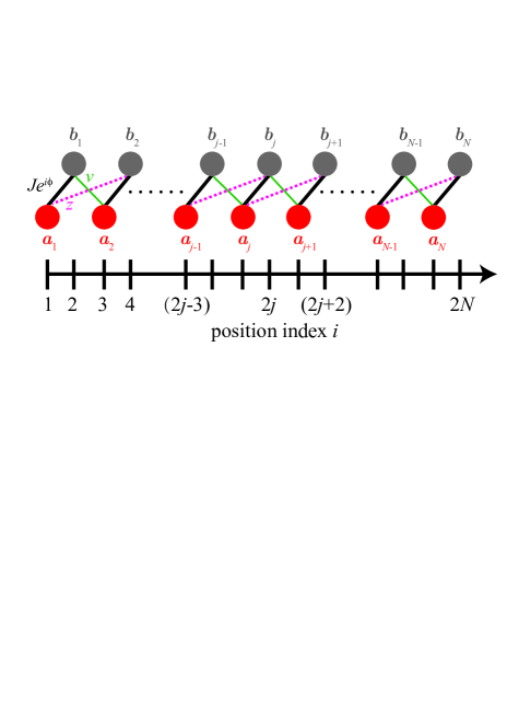
Figure 1: (Color online) Schematic diagram of a generalized SSH model based on an optomechanical array. $a_{j}$ and $b_{j}$ denote the cavity and mechanical modes respectively, and they are coupled with three different hopping amplitudes $Je^{i\phi}$ (bold black lines), $v$ (thin green lines) and $z$ (red dashed lines). The optomechanical array can be implemented by an array of coupled optical microdisks LinPRL09 ; MLiNatPhot09 ; WeisSci10 ; MZhangPRL15 , on-chip superconducting circuit electromechanical cavities TeufelNat11 ; MasselNC12 ; PalomakiSci13 ; SuhSci14 , and optomechanical crystals EichenfieldNat09 ; Safavi-NaeiniPRL14 .

We propose to implement a generalized SSH model by an optomechanical array with $N$ cavity modes and $N$ mechanical modes, which are coupled only by optomechanical interactions, without hopping of photons (or phonons) between neighboring cavity modes (mechanical modes). The Hamiltonian of the optomechanical array is ($\hbar=1$)

$$H_{0}=\sum_{j=1}^{N}\left(\omega_{c,j}a_{j}^{{\dagger}}a_{j}+\omega_{m,j}b_{j}^{{\dagger}}b_{j}+H_{j}\right),$$ (1)

with

$$H_{1} = \left(g_{1,0}b_{1}^{{\dagger}}+g_{1,+}b_{2}^{{\dagger}}\right)a_{1}^{{\dagger}}a_{1}$$ (2)

$$+\left(\Omega_{1,0}e^{i\omega_{1,0}t}+\Omega_{1,+}e^{i\omega_{1,+}t}\right)a_{1}+\mathrm{H.c.},$$

for the first cavity mode,

$$H_{N} = \left(g_{N,0}b_{N}^{{\dagger}}+g_{N,-}b_{N-1}^{{\dagger}}\right)a_{N}^{{\dagger}}a_{N}$$ (3)

$$+\left(\Omega_{N,0}e^{i\omega_{N,0}t}+\Omega_{N,-}e^{i\omega_{N,-}t}\right)a_{N}+\mathrm{H.c.},$$

for the last cavity mode, and

$$H_{j} = \left(g_{j,0}b_{j}^{{\dagger}}+g_{j,+}b_{j+1}^{{\dagger}}+g_{j,-}b_{j-1}^{{\dagger}}\right)a_{j}^{{\dagger}}a_{j}$$ (4)

$$+\left(\Omega_{j,0}e^{i\omega_{j,0}t}+\Omega_{j,+}e^{i\omega_{j,+}t}+\Omega_{j,-}e^{i\omega_{j,-}t}\right)a_{j}$$

$$+\mathrm{H.c.},$$

for the $j$th cavity mode ($1<j<N$), where $a_{j}$ ($a_{j}^{{\dagger}}$) is the bosonic annihilation (creation) operator of the $j$th cavity mode ($j=1,2,\cdots,N$) with resonant frequency $\omega_{c,j}$, $b_{j}$ ($b_{j}^{{\dagger}}$) is the bosonic annihilation (creation) operator of the $j$th mechanical mode with resonant frequency $\omega_{m,j}$, and $g_{j,0}$ ($g_{j,\pm}$) is the optomechanical coupling strength between the $j$th cavity mode and the $j$th mechanical mode (the $(j\pm 1)$th mechanical mode). The $j$th cavity mode is driven by a three-tone laser at frequencies $\omega_{j,0}=\omega_{c,j}-\omega_{m,j}$ and $\omega_{j,\pm}=\omega_{c,j}-\omega_{m,j\pm 1}$ with amplitudes $\Omega_{j,0}$ and $\Omega_{j,\pm}$ in the well resolved sidebands regime ($\omega_{m,j}\gg\{\kappa_{j},\gamma_{j}\}$, where $\kappa_{j}$ is the decay rate of the $j$th cavity mode, and $\gamma_{j}$ is the damping rate of the $j$th mechanical mode).

To linearize the Hamiltonians in Eqs. (2)-(4), we can write the operator for each cavity modes as the sum of its classical mean value and quantum fluctuation operator as $a_{j}\rightarrow\alpha_{j}(t)+a_{j}$. The classical part $\alpha_{j}(t)$ can be given approximately as $\alpha_{j}(t)\approx\alpha_{j,0}e^{i\omega_{j,0}t}+\alpha_{j,+}e^{i\omega_{j,+}t}+\alpha_{j,-}e^{i\omega_{j,-}t}$, where the classical amplitude $\alpha_{j,0}$ ($\alpha_{j,\pm}$) is determined by solving the classical equation of motion with only cavity drive $\Omega_{j,0}$ ($\Omega_{j,\pm}$) at frequency $\omega_{j,0}$ ($\omega_{j,\pm}$). We assume that: (i) min$\left[\left|\alpha_{j,0}\right|,|\alpha_{j,\pm}|\right]\gg 1$, so that we can only keep the first-order terms in the small quantum fluctuation operators; (ii) min$\left[\omega_{m,j},\left|\omega_{m,j}-\omega_{m,j^{\prime}}\right|_{j^{\prime}=j\pm 1}\right]\gg\mathrm{max}\left[\left|g_{j,0}\alpha_{j,0}\right|,\left|g_{j,\pm}\alpha_{j,\pm}\right|\right]$, such that the counter-rotating terms can be neglected safely; in the interaction picture with respect to $H_{\mathrm{rot}}=\sum_{j=1}^{N}\left[\omega_{c,j}a_{j}^{{\dagger}}a_{j}+\omega_{m,j}b_{j}^{{\dagger}}b_{j}\right]$, the linearized form of the interaction Hamiltonians in Eqs. (2)-(4) are obtained as

$$H_{1}=Je^{i\phi}a_{1}^{{\dagger}}b_{1}+za_{1}^{{\dagger}}b_{2}+\mathrm{H.c.},$$ (5)

$$H_{N}=Je^{i\phi}a_{N}^{{\dagger}}b_{N}+za_{N}^{{\dagger}}b_{N-1}+\mathrm{H.c.},$$ (6)

$$H_{j}=Je^{i\phi}a_{j}^{{\dagger}}b_{j}+za_{j}^{{\dagger}}b_{j+1}+va_{j}^{{\dagger}}b_{j-1}+\mathrm{H.c.},$$ (7)

where $Je^{i\phi}\equiv g_{j,0}\alpha_{j,0}$, $v\equiv g_{j,-}\alpha_{j,-}$, and $z\equiv g_{j,+}\alpha_{j,+}$. Without loss of generality, we assume that $J$, $v$ and $z$ are real coupling strengths and the effect of the phase factor $\phi$ can be observed experimentally.

In summary, by substituting Eqs. (5)-(7) into Eq. (1), the linearized Hamiltonian for the optomechanical array in the interaction picture with respect to $H_{\mathrm{rot}}=\sum_{j=1}^{N}\left[\omega_{c,j}a_{j}^{{\dagger}}a_{j}+\omega_{m,j}b_{j}^{{\dagger}}b_{j}\right]$ is given by

$$H=\sum_{j=1}^{N}Je^{i\phi}a_{j}^{{\dagger}}b_{j}+\sum_{j=1}^{N-1}\left(va_{j+1}^{{\dagger}}b_{j}+zb_{j+1}^{{\dagger}}a_{j}\right)+\mathrm{H.c.},$$ (8)

as schematically shown in Fig. 1. The linearized Hamiltonian for the optomechanical array shows a generalized SSH model with hopping amplitude $z\neq 0$ between the $j$th cavity mode and $(j+1)$th mechanical mode. When the coupling strength $z=0$, the Hamiltonian for the optomechanical array becomes the well-known SSH model AsbothBook16 .

III Topological phase transition

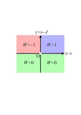
Figure 2: (Color online) Phase diagram of the generalized SSH model with $\phi=0$. The winding number is: $W=1$ if $z>v$ and $z+v>J$; $W=-1$ if $z<v$ and $z+v>J$; or $W=0$ if $z+v<J$.

To study the topological phase transition in the generalized SSH model, we set a periodic boundary condition, so the linearized Hamiltonian for one-dimensional optomechanical array can be redefined as

$$H^{\prime} = \sum_{j=1}^{N}\left(Je^{i\phi}a_{j}^{{\dagger}}b_{j}+va_{\left(j\text{ }\mathrm{mod}\text{ }N\right)+1}^{{\dagger}}b_{j}+zb_{\left(j\text{ }\mathrm{mod}\text{ }N\right)+1}^{{\dagger}}a_{j}\right)$$ (9)

$$+\mathrm{H.c.},$$

where $\mathrm{mod}$ stands for the modular calculation. By using the for Fourier transform for $a_{j}$ and $b_{j}$ as

$$\left(\begin{array}[]{c}a_{j}\\ b_{j}\end{array}\right)=\sum_{k}e^{-ikj}\left(\begin{array}[]{c}a_{k}\\ b_{k}\end{array}\right),$$ (10)

then the Hamiltonian in Eq. (9) can be rewritten as

$$H^{\prime}=\sum_{k}\left(\begin{array}[]{cc}a_{k}^{{\dagger}}&b_{k}^{{\dagger}}\end{array}\right)H^{\prime}\left(k\right)\left(\begin{array}[]{c}a_{k}\\ b_{k}\end{array}\right)$$ (11)

with

$$H^{\prime}\left(k\right)=\left(\begin{array}[]{cc}0&h\left(k\right)\\ h^{\ast}\left(k\right)&0\end{array}\right)$$ (12)

and

$$h\left(k\right)=Je^{i\phi}+ve^{-ik}+ze^{ik},$$ (13)

where $k$ is the wavenumber in the first Brillouin zone. The dispersion relation of the generalized SSH model with periodic boundary conditions is given by

$$E=\pm\left|Je^{i\phi}+ve^{-ik}+ze^{ik}\right|.$$ (14)

The winding number, which characterizes the topological invariant of an insulating Hamiltonian, is defined by AsbothBook16

$$W=\frac{1}{2\pi i}\int_{-\pi}^{\pi}dk\frac{d\ln h\left(k\right)}{dk}.$$ (15)

For the generalized SSH model with $h\left(k\right)$ given by Eq. (13), the winding number is either $0$ or $\pm 1$, depending on the parameters. When the phase factor $\phi=0$, see Fig. 2, the winding number is: (i) $W=1$ if $z>v$ and $z+v>J$; (ii) $W=-1$ if $z<v$ and $z+v>J$; (iii) $W=0$ if $z+v<J$.

The Hamiltonian for the generalized SSH model in the momentum space can be written in an alternative form as

$$H^{\prime}\left(k\right) = \mathbf{d}\left(k\right)\cdot\widehat{\mathbf{\sigma}}$$ (16)

$$= d_{x}\left(k\right)\widehat{\sigma}_{x}+d_{y}\left(k\right)\widehat{\sigma}_{y}+d_{z}\left(k\right)\widehat{\sigma}_{z},$$

where $\widehat{\sigma}_{x}$, $\widehat{\sigma}_{y}$, and $\widehat{\sigma}_{z}$ are the Pauli matrices, and

$$d_{x}\left(k\right)=J\cos\phi+v\cos k+z\cos k,$$ (17)

$$d_{y}\left(k\right)=J\sin\phi-v\sin k+z\sin k,$$ (18)

$$d_{z}\left(k\right)=0.$$ (19)

The winding number can also be obtained graphically by counting the number of times the loop winds around the origin of the $d_{x},d_{y}$ plane.

We show the dispersion relation and the path that the endpoint of the vector $\mathbf{d}\left(k\right)$ traces out in Fig. 3 for $v>z$. As the wavenumber runs through the Brillouin zone, $k=0\rightarrow 2\pi$, the path that the endpoint of the vector $\mathbf{d}\left(k\right)$ is a closed ellipse of long axis $v+z$ and short axis $|v-z|$ on the $d_{x},d_{y}$ plane, centered at $\left(J,0\right)$, and the endpoint rotates around the origin clockwise. It is clear that the winding number is $W=-1$ when $z+v>J$ for $z<v$, and the winding number is $W=0$ when $z+v<J$.

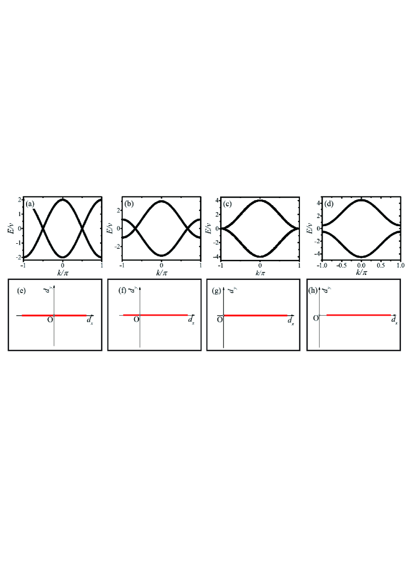
Figure 12: (Color online) Dispersion relations of the generalized SSH model with different hopping amplitude $J$: (a) $J=0$; (b) $J/v=1$; (c) $J/v=2$; (d) $J/v=2.5$. (e)-(h) The paths of the endpoint of the vector $\textbf{d}(k)$ corresponding to (a)-(d) are shown on the $d_{x},d_{y}$ plane as the wavenumber is sweeped across the Brillouin zone, $k=0\rightarrow 2\pi$. The other parameters are $z/v=1$ and $\phi=0$.

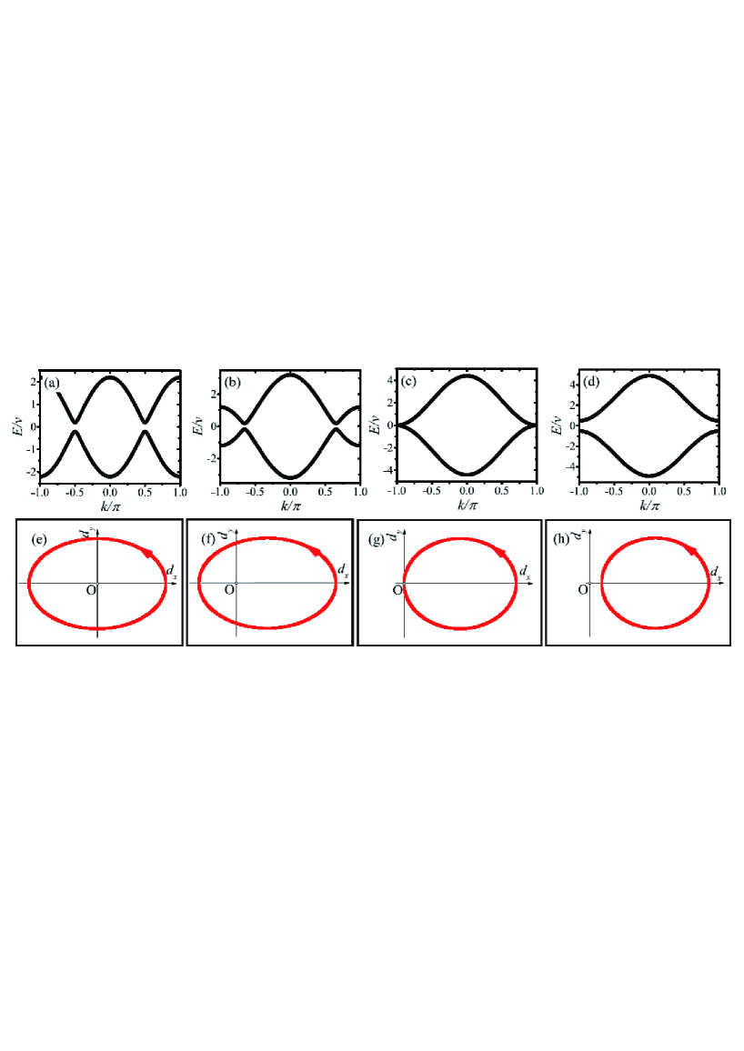
Figure 13: (Color online) Dispersion relations of the generalized SSH model with different hopping amplitude $J$: (a) $J=0$; (b) $J/v=1$; (c) $J/v=2.2$; (d) $J/v=2.7$. (e)-(h) The paths of the endpoint of the vector $\textbf{d}(k)$ corresponding to (a)-(d) are shown on the $d_{x},d_{y}$ plane as the wavenumber is sweeped across the Brillouin zone, $k=0\rightarrow 2\pi$. The other parameters are $z/v=1.2$ and $\phi=0$.

Two more figures about the dispersion relation and the path that the endpoint of the vector $\mathbf{d}\left(k\right)$ traces are shown in Figs. 12 and 13, given in the Appendix. In Fig. 12, as $v=z$, the path of the endpoint of the vector $\mathbf{d}\left(k\right)$ becomes a straight line on the $d_{x}$-axis. In Fig. 13, as $v<z$, similarly to the case for $v>z$, the path of the endpoint of the vector $\mathbf{d}\left(k\right)$ is also a closed ellipse of long axis $v+z$ and short axis $|v-z|$ on the $d_{x},d_{y}$ plane, centered at $\left(J,0\right)$. However, the endpoint rotates around the origin counterclockwise for $v<z$. So we can conclude that the winding number is (i) $W=1$ when $z+v>J$ and $v<z$; (ii) $W=-1$ when $z+v>J$ and $v>z$; (iii) $W=0$ when $z+v<J$. These consist with the results shown in Fig. 2.

The above results are obtained under the condition for $\phi=0$. In Fig. 4, we show that the topological phase transition can be induced by tuning the phase $\phi$. For $\phi\neq 0$, the path that the endpoint of the vector $\mathbf{d}\left(k\right)$ is centered at $\left(J\cos\phi,J\sin\phi\right)$. The topological phase transition appears when $E=0$, as shown in Fig. 4(b), which gives the critical phase $\phi_{c}$ as

$$\tan\phi_{c}=\frac{z-v}{z+v}\tan k,$$ (20)

where

$$\cos^{2}k=\frac{J^{2}-\left(z-v\right)^{2}}{\left(z+v\right)^{2}-\left(z-v\right)^{2}}.$$ (21)

As $v>z$, we have $W=-1$ for $\phi=0$ in Fig. 4(a); we have $W=0$ for $\phi=0.1$ in Fig. 4(c); the winding number is not well-defined in the critical point for $\phi=\phi_{c}\approx 0.04$ as shown in Fig. 4(b). The paths [see Fig. 4(d)-(f)] that the endpoint of the vector $\mathbf{d}\left(k\right)$ traces, corresponding to dispersion relation [see Fig. 4(a)-(c)] for $v<z$, show the phase transition from $W=1$ to $W=0$ by tuning $\phi$.

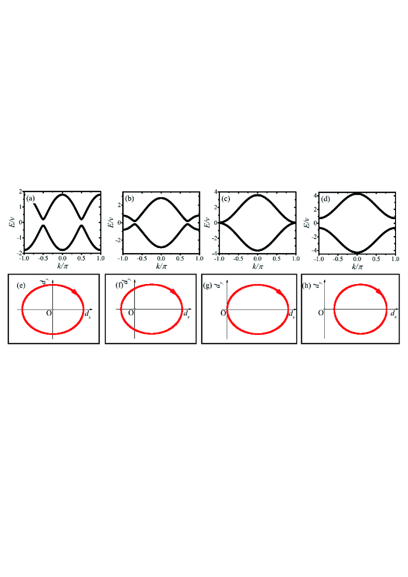
Figure 3: (Color online) Dispersion relations of the generalized SSH model with different hopping amplitude $J$: (a) $J=0$; (b) $J/v=1$; (c) $J/v=1.8$; (d) $J/v=2.5$. (e)-(h) The paths of the endpoint of the vector $\textbf{d}(k)$ corresponding to (a)-(d) are shown on the $d_{x},d_{y}$ plane as the wavenumber is sweeped across the Brillouin zone, $k=0\rightarrow 2\pi$. The other parameters are $z/v=0.8$ and $\phi=0$.

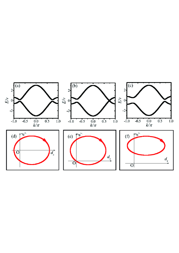
Figure 4: (Color online) Dispersion relations of the generalized SSH model for hopping amplitude $J/v=1.2$ with different phase: (a) $\phi=0$; (b) $\phi=\phi_{c}\approx 0.04$; (c) $\phi=0.1$. (d)-(f) The paths of the endpoint of the vector $\textbf{d}(k)$, corresponding to (a)-(c), are shown on the $d_{x},d_{y}$ plane as the wavenumber is sweeped across the Brillouin zone, $k=0\rightarrow 2\pi$. The other parameter is $z/v=0.8$.

IV Edge states

We now study how to demonstrate topologically protected edge states in the optomechanical array of an open chain under single-particle excitation. To be specific, we choose an open chain of $N=8$ for the optomechanical array, then the wave function for the Hamiltanion in Eq. (8) under single-particle excitation can be defined as

$$\left|\Psi\left(t\right)\right\rangle=\sum_{j=1}^{N}\left[c_{2j-1}\left(t\right)\left|a_{j}\right\rangle+c_{2j}\left(t\right)\left|b_{j}\right\rangle\right],$$ (22)

where $P_{2j-1}\left(t\right)=\left|c_{2j-1}\left(t\right)\right|^{2}$ and $P_{2j}\left(t\right)=\left|c_{2j}\left(t\right)\right|^{2}$ denote the occupying probabilities in the $j$th cavity mode and $j$th mechanical mode, respectively. For simplicity, we define $P_{i}\left(t\right)=\left|c_{i}\left(t\right)\right|^{2}$ with the position index $i$ shown in Fig. 1.

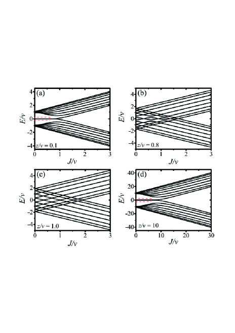
Figure 5: (Color online) Energy spectrum of the open chain optomechanical array for $N=8$ as a function the intracell hopping amplitude $J$ for different intercell hopping amplitude $z$: (a) $z/v=0.1$; (b) $z/v=0.8$; (c) $z/v=1.0$; (d) $z/v=10$. The phase factor is $\phi=0$.

The energy spectrum of a generalized SSH model with $N=8$ is shown in Fig. 5. Under the conditions $z\ll v$ or $z\gg v$, see Figs. 5(a) and 5(d), the energy spectrum of a generalized SSH model is similar to that of the standard SSH model. However, due to the level crossings for the nearest neighbor eigenmodes and avoided level crossings for the next-nearest neighbor eigenmodes, there are four ($N/2$) degenerate points of the zero-energy modes within the interval $0<J<z+v$, as shown in Figs. 6(a) and 6(b), which are the local enlarged drawings of the boxes with red dashed-line in Figs. 5(a) and 5(d). When $z=0.8v$, as shown Fig. 5(b), there are degenerate points for the nearest neighbor eigenmodes and avoided level crossings for the next-nearest neighbor eigenmodes. But when $z=v$, as shown Fig. 5(c), all the avoided level crossings for the next-nearest neighbor eigenmodes disappear.

The probability distributions of the eigenstates, corresponding to the points marked out in Figs. 6(a) and 6(b), are shown in Figs. 6(c)-6(f). Apparently, the probability distributions of the eigenstates are localized. We define four edge states, i.e., left cavity (LC), left mechniacal (LM), right cavity (RC), right mechniacal (RM) edge states, as

$$\left|LC\right\rangle=\sum_{j=1}^{N}c_{1}e^{-2\left(j-1\right)/\xi}\left|a_{j}\right\rangle,$$ (23)

$$\left|LM\right\rangle=\sum_{j=1}^{N}c_{2}e^{-2\left(j-1\right)/\xi}\left|b_{j}\right\rangle,$$ (24)

$$\left|RC\right\rangle=\sum_{j=1}^{N}c_{2N-1}e^{2\left(j-N\right)/\xi}\left|a_{j}\right\rangle,$$ (25)

$$\left|RM\right\rangle=\sum_{j=1}^{N}c_{2N}e^{2\left(j-N\right)/\xi}\left|b_{j}\right\rangle,$$ (26)

where $\xi>0$ is the localization length determined by the relative size of the hopping amplitudes $v$, $z$, and $J$. When $v\gg z$ and $J\ll v+z$ (corresponding to the winding number $W=-1$ under the periodic boundary condition), as shown in Figs. 6(c) and 6(d), the edge states are the hybridized states of the LC edge state and RM edge state. A concise physical picture for the edge states with $v\gg z$ and $J\ll v+z$ is shown in Fig. 6(g), where dimers are formed between $b_{j}$ and $a_{j+1}$, and $a_{1}$ and $b_{N}$ are isolated from the others. Similarly, when $v\ll z$ and $J\ll v+z$ (corresponding to the winding number $W=1$ under the periodic boundary condition), the edge states are the hybridized states of the LM edge state and RC edge state, as shown in Figs. 6(e) and 6(f). The physical picture for the edge states with $v\ll z$ and $J\ll v+z$ is shown in Fig. 6(h), where dimers are formed between $a_{j}$ and $b_{j+1}$, and $b_{1}$ and $a_{N}$ are isolated from the others. When $J>v+z$ (corresponding to the winding number $W=0$ under the periodic boundary condition), dimers are formed between $a_{j}$ and $b_{j}$, and no modes are isolated from the others (the physical picture is not shown in the text). Thus, there is no edge states when $J>v+z$.

Figure 7 shows the time evolution of the probability distribution for the generalized SSH model with the open boundary condition (i.e., an open chain with $N=8$): (a)-(e) an excitation is injected at the first cavity mode $P_{1}(0)=1$ for $z=v/10$, or (f)-(j) an excitation is injected at the first mechanical mode $P_{2}(0)=1$ for $z=10v$. From these figures, we can see that: (i) When $J=z\ll v$ or $J=v\ll z$, as shown in Figs. 7(a) and 7(f), the excitation almost localizes in the injected cavity or mechanical mode like a soliton for a long time. With a larger value of $J$ (still with $J<z+v$), as shown in Figs. 7(b) and 7(g), the excitation spreads to the nearest neighbor modes and the localization of the excitation becomes weaker. (ii) When $J=z+v$ (i.e., the topological phase transition point), as shown in Figs. 7(d) and 7(i), the excitation, oscillating like a soliton, travels in the open chain and reflects back at the ends. The traveling speed (the period of oscillation) is dependent on the hopping amplitudes: the excitation travels much faster in Fig. 7(i) with $z/v=10$ and $J/v=11$ than in Fig. 7(d) with $z/v=0.1$ and $J/v=1.1$. As $J$ is away from the topological phase transition point ($J\neq z+v$), as shown in Figs. 7(c) and 7(e) [or Figs. 7(h) and 7(j)], the distribution of the traveling excitation disperses much faster than the case with $J=z+v$. That is to say, the optimal condition for the excitation traveling like a soliton with less dispersion in the open chain is the system working at the critical point $J=z+v$.

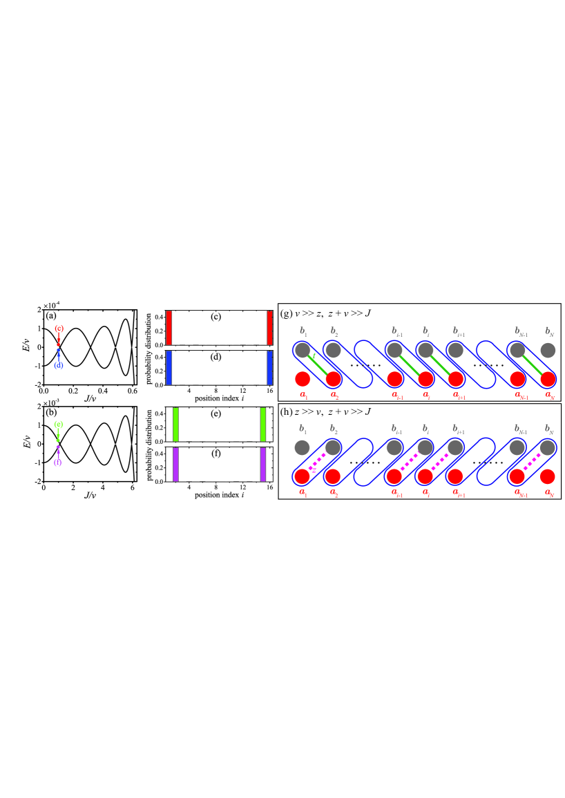
Figure 6: (Color online) (a) and (b) are the local enlarged drawings of 5(a) and 5(d). (c)-(f) show the probability distributions of the eigenfunctions corresponding to the points shown in (a) and (b). (g) Edge states appear at $a_{1}$ and $b_{N}$ corresponding to (c) and (d) for $v\gg z$ and $J\ll v+z$. (h) Edge states appear at $b_{1}$ and $a_{N}$ corresponding to (e) and (f) for $z\gg v$ and $J\ll v+z$.

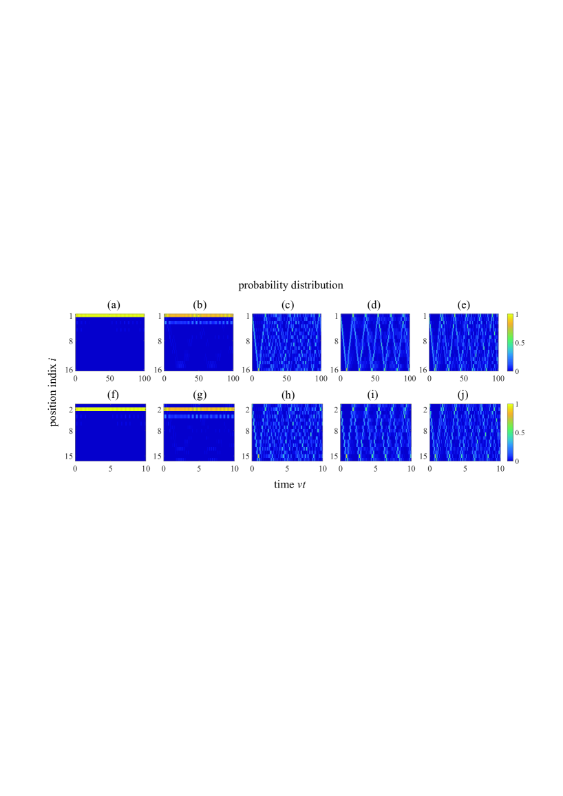
Figure 7: (Color online) Time evolution of the probability distribution of an open chain for $N=8$: (a)-(e) $z/v=0.1$ and $P_{1}(0)=1$, with (a) $J/v=0.1$, (b) $J/v=0.3$, (c) $J/v=1.0$, (d) $J/v=1.1$, (e) $J/v=1.2$; (f)-(j) $z/v=10$ and $P_{2}(0)=1$, with (f) $J/v=1$, (g) $J/v=3$, (h) $J/v=10$, (i) $J/v=11$, (j) $J/v=12$. The phase factor is $\phi=0$.

V Adiabatic particle pumping

As shown in the previous section, once an excitation is injected at one edge, it will stay there like a stationary state. However, we will show that it is possible to transfer the edge states from one to another by adiabatic pumping with periodically modulated optomechanical array with Hamiltonian as

$$H = \sum_{j=1}^{N}\left[u\left(t\right)a_{j}^{{\dagger}}a_{j}+J\left(t\right)a_{j}^{{\dagger}}b_{j}\right]$$ (27)

$$+\sum_{j=1}^{N-1}\left[v\left(t\right)a_{j+1}^{{\dagger}}b_{j}+z\left(t\right)b_{j+1}^{{\dagger}}a_{j}\right]+\mathrm{H.c.},$$

where $u\left(t\right)$ is the detuning between the cavity modes and mechanical modes. The modulated optomechanical array can be realized by modulating the frequencies and strengths of the driving fields.

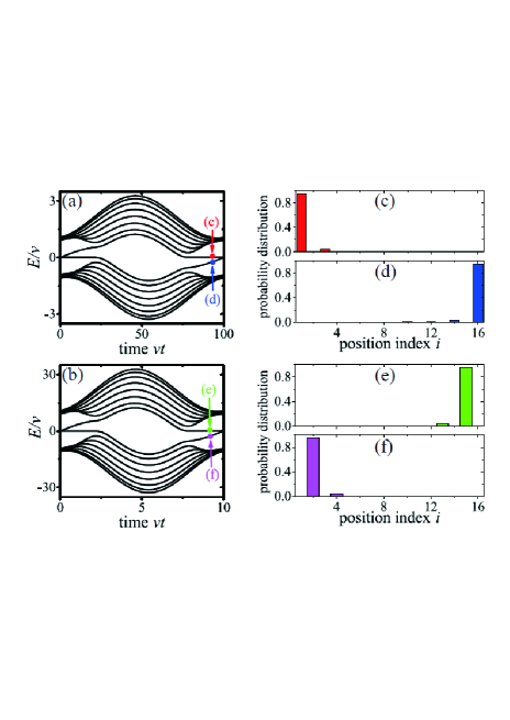
Figure 8: (Color online) Instantaneous spectrum of the open chain optomechanical array for $N=8$. The time dependent pump sequence is defined in Eq. (28), with (a) $z/v=0.1$, $A/v=1.1$, and $\omega/v=2\pi/100$; (b) $z/v=10$, $A/v=11$, and $\omega/v=2\pi/10$. (c)-(f) show the probability distributions of the edge states corresponding to the points shown in (a) and (b). The phase factor is $\phi=0$.

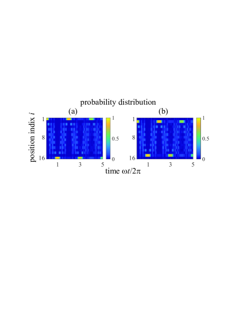
Figure 9: (Color online) Time evolution of the probability distribution for an open chain of $N=8$. The time dependent pump sequence is defined in Eq. (28), with (a) $z/v=0.1$, $A/v=1.1$, $\omega/v=2\pi/100$, and $P_{1}(0)=1$; (b) $z/v=10$, $A/v=11$, $\omega/v=2\pi/10$, and $P_{2}(0)=1$. The phase factor is $\phi=0$.

First, we consider a smooth modulation sequence as

$$\left\{\begin{array}[]{c}u\left(t\right)=\frac{A}{2}\sin\left(\omega t\right),\\ J\left(t\right)=A\left[1-\cos\left(\omega t\right)\right],\\ v\left(t\right)=\mathrm{const.},\\ z\left(t\right)=\mathrm{const.},\end{array}\right.$$ (28)

where, $u(t)$ and $J(t)$ are modulated periodically with amplitudes $A/2$ and $A$, and frequency $\omega$; $u(t)$ and $J(t)$ are maintained constant.

The instantaneous spectrum of the Hamiltonian in Eq. (27) with time dependent pump sequence defined in Eq. (28) is shown in Figs. 8(a) and 8(b). In Figs. 8(c)-8(f), the probability distributions of eigenstates corresponding to the points shown in Figs. 8(a) and 8(b), are approximately the edge states defined in Eqs. (23)-(26) as: Fig. 8(c), LC edge state; Fig. 8(d), RM edge state; Fig. 8(e), RC edge state; Fig. 8(f), LM edge state. When the adiabatic approximation holds, the system will stay in the same eigenstate. Fig. 8(a) shows how a LC edge state is adiabatically pumped to the RM edge state during a pumping cycle, in the mean while Fig. 8(b) shows how a RC edge state is adiabatically pumped to the LM edge state within a pumping cycle.

The dynamics of the probability distributions for an open chain with a time dependent pump sequence defined in Eq. (28) are obtained numerically. As shown in Fig. 9(a), the excitation at the first cavity mode (LC edge state) quickly expands into the bulk, and then the probability refocuses on the $N$th mechanical mode (RM edge state) at the end of the first pumping cycle. In the second pumping cycle, the probability expands into the bulk again and refocuses on the first cavity mode (LC edge state) at the end of the second pumping cycle. Similarly, as shown in Fig. 9(b), the excitation at the first mechanical mode (LM edge state) expands into the bulk and refocuses on the $N$th cavity mode (RC edge state) at the end of the first pumping cycle, and then the probability expands into the bulk again and refocuses on the first mechanical mode (LM edge state) at the end of the second pumping cycle. These results are well consistent with the instantaneous spectrum in the adiabatic limit, as shown in Fig. 8. However, due to the Landau Zener transition occurs at the degenerate points $\omega t=2n\pi$ ($n$ is positive integer), the periodical behavior of the probability distribution becomes less well-resolved in the following cycles.

As shown in Figs. 8 and 9, with time dependent pump sequence defined in Eq. (28), the LC edge state can be pumped adiabatically to the RM edge state, and the LM edge state can be pumped adiabatically to the RC edge state, and vice versa. However, the LC edge state can not be pumped adiabatically to the RC edge state, and the LM edge state can not be pumped adiabatically to the RM edge state. Now, we consider another smooth modulation sequence to realizing the adiabatical pumping between the the LC (LM) edge state and the RC (RM) edge state. The smooth modulation sequence is defined by

$$\left\{\begin{array}[]{c}u\left(t\right)=\frac{A}{2}\sin\left(\omega t\right),\\ J\left(t\right)=\mathrm{const.},\\ v\left(t\right)=A\left[1+\cos\left(\omega t\right)\right],\\ z\left(t\right)=A\left[1-\cos\left(\omega t\right)\right].\end{array}\right.$$ (29)

Here, $u(t)$, $v(t)$ and $z(t)$ are modulated periodically with amplitudes $A/2$ and $A$, and frequency $\omega$, while $J(t)$ is maintained constant.

The instantaneous spectrum of the Hamiltonian in Eq. (27) with time dependent pump sequence defined in Eq. (29) is shown in Fig. 10(a). In Figs. 10(b)-10(e), the probability distributions of eigenstates corresponding to the points shown in Fig. 10(a), are approximately the edge states defined in Eqs. (23)-(26) as: Fig. 10(b) LC edge state; Fig. 10(c) RM edge state; Fig. 10(d) LM edge state; Fig. 10(e) RC edge state. When the adiabatic approximation holds, the system will stay in the same eigenstate. Fig. 10(a) shows how a LC edge state is adiabatically pumped to the RC edge state during a pumping cycle, in the mean while, a LM edge state is adiabatically pumped to the RM edge state within a pumping half-cycle.

The dynamics of the probability distribution for an open chain with a time dependent pump sequence defined in Eq. (29) are shown in Fig. 11. In Fig. 11(a), the excitation at the first cavity mode (LC edge state) quickly expands into the bulk, and then the probability refocuses on the $N$th cavity mode (RC edge state) at the end of the first pumping half-cycle. In the second pumping half-cycle, the probability expands into the bulk again and refocuses on the first cavity mode (LC edge state) at the end of the first pumping cycle. Similarly, as shown in Fig. 11(b), the excitation at the first mechanical mode (LM edge state) expands into the bulk and refocuses on the $N$th mechanical mode (RM edge state) at the end of the first pumping half-cycle, and then the probability expands into the bulk again and refocuses on the first mechanical mode (LM edge state) at the end of the first pumping cycle. These results are consistent well with the instantaneous spectrum in the adiabatic limit, as shown in Fig. 10. However, due to the Landau Zener transition occurs at the degenerate points $\omega t=n\pi$ ($n$ is positive integer), the periodical behavior of the probability distribution becomes less well-resolved in the following cycles.

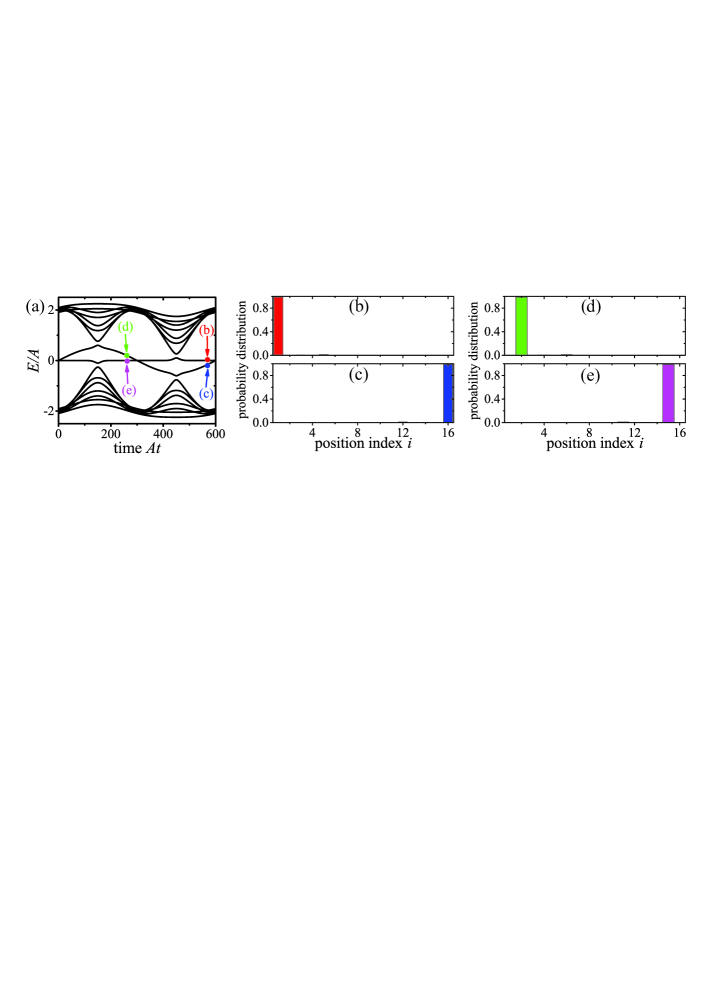
Figure 10: (Color online) Instantaneous spectrum of the open chain optomechanical array for $N=8$, $J/A=0.1$, and $\phi=0$. The time dependent pump sequence is defined in Eq. (29) with $\omega/A=2\pi/600$. (b)-(e) show the probability distributions of the edge states corresponding to the points shown in (a).

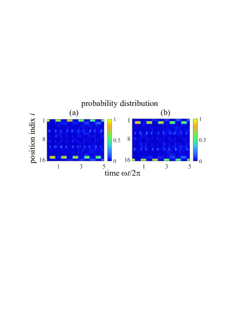
Figure 11: (Color online) Time evolution of the probability distribution for an open chain of $N=8$. The time dependent pump sequence is defined in Eq. (29) with $\omega/A=2\pi/600$, (a) $P_{1}(0)=1$; (b) $P_{16}(0)=1$. The other parameters are $J/A=0.1$ and $\phi=0$.

Overall, with time dependent pump sequence defined in Eq. (28), the LC edge state can be pumped adiabatically to the RM edge state, and the LM edge state can be pumped adiabatically to the RC edge state; with time dependent pump sequence defined in Eq. (29), the LC edge state can be pumped adiabatically to the RC edge state, and the LM edge state can be pumped adiabatically to the RM edge state. Therefore, the four edge states can be pumped from one to another adiabatically with smooth modulation sequence.

VI Conclusions

In summary, we have proposed an implementation of a generalized SSH model based on optomechanical arrays. This generalized SSH model supports two distinct nontrivial topological phases, and the transitions between different phases can be observed by tuning the strengths and phases of the effective optomechanical interactions. Dynamic control of the effective optomechanical interactions can be realized by tuning the strengths and phases of external driving lasers, which allows for dynamic control of the topological phase transitions. Moreover, four types of edge states can be generated in the generalized SSH model of an open chain under single-particle excitation, and the dynamical behaviors of the excitation in the open chain depend on the topological properties under the periodic boundary condition. We show that the edge states can be pumped adiabatically along the optomechanical arrays by periodically modulating the amplitudes and frequencies of the driving fields. Our results can be applied to control the transport of photons and phonons, and the generalized SSH model based on the optomechanical arrays provides us a tunable platform to engineer topological phases for photons and phonons.

Appendix A Supplemental dispersion relations

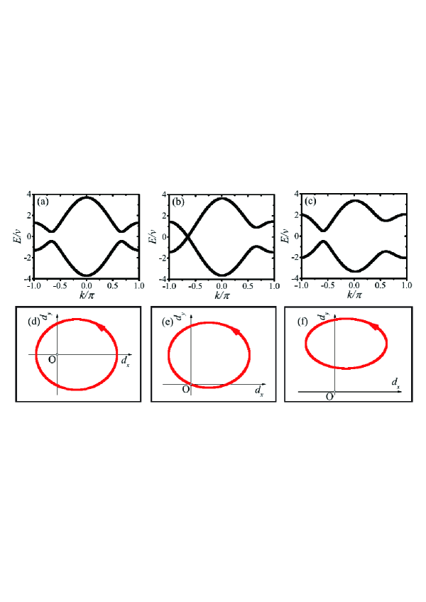
Figure 14: (Color online) Dispersion relations of the generalized SSH model for hopping amplitude $J/v=1.2$ with different phase: (a) $\phi=0$; (b) $\phi=\phi_{c}\approx 0.12$; (c) $\phi=0.3$. (d)-(f) The paths of the endpoint of the vector $\textbf{d}(k)$ corresponding to (a)-(c) are shown on the $d_{x},d_{y}$ plane as the wavenumber is sweeped across the Brillouin zone, $k=0\rightarrow 2\pi$. The other parameter is $z/v=1.5$.

Acknowledgement

X.W.X. is supported by the National Natural Science Foundation of China (NSFC) under Grants No.11604096 and the Startup Foundation for Doctors of East China Jiaotong University under Grant No. 26541059. Y.J.Z. is supported by the China Postdoctoral Science Foundation under grant No. 2017M620945. A.X.C. is supported by NSFC under Grant No. 11775190. Y.X.L. is supported by the National Basic Research Program of China(973 Program) under Grant No. 2014CB921401, the Tsinghua University Initiative Scientific Research Program, and the Tsinghua National Laboratory for Information Science and Technology (TNList) Cross-discipline Foundation.

References

- (1) T. J. Kippenberg and K. J. Vahala, Cavity Optomechanics: Back-Action at the Mesoscale, Science 321, 1172 (2008).
- (2) F. Marquardt and S. M. Girvin, Optomechanics, Physics 2, 40 (2009).
- (3) M. Aspelmeyer, P. Meystre, and K. Schwab, Quantum optomechanics, Phys. Today 65(7), 29 (2012).
- (4) M. Aspelmeyer, T. J. Kippenberg, and F. Marquardt, Cavity Optomechanics, Rev. Mod. Phys. 86, 1391 (2014).
- (5) M. Metcalfe, Applications of cavity optomechanics, Appl. Phys. Rev. 1, 031105 (2014).
- (6) Y. L. Liu, C. Wang, J. Zhang, and Y. X. Liu, Cavity optomechanics: Manipulating photons and phonons towards the single-photon strong coupling, Chin. Phys. B 27, 024204 (2018).
- (7) Q. Lin, J. Rosenberg, X. Jiang, K. J. Vahala, and O. Painter, Mechanical Oscillation and Cooling Actuated by the Optical Gradient Force, Phys. Rev. Lett. 103, 103601 (2009).
- (8) M. Li, W. H. P. Pernice, and H. X. Tang, Tunable bipolar optical interactions between guided lightwaves, Nature Photon. 3, 464 (2009).
- (9) S. Weis, R. Rivière. S. Deléglise, E. Gavartin, O. Arcizet, A. Schliesser, and T. J. Kippenberg, Optomechanically Induced Transparency, Science 330, 1520 (2010).
- (10) M. Zhang, S. Shah, J. Cardenas, and M. Lipson, Synchronization and Phase Noise Reduction in Micromechanical Oscillator Arrays Coupled through Light, Phys. Rev. Lett. 115, 163902 (2015).
- (11) J. D. Teufel, D. Li, M. S. Allman, K. Cicak, A. J. Sirois, J. D. Whittaker, and R. W. Simmonds, Circuit cavity electromechanics in the strong-coupling regime, Nature (London) 471, 204 (2011).
- (12) F. Massel, S. Un Cho, J.-M. Pirkkalainen, P. J. Hakonen, T. T. Heikkilä, and M. A. Sillanpää, Multimode circuit optomechanics near the quantum limit, Nat. Commun. 3, 987 (2012).
- (13) T. A. Palomaki, J. D. Teufel, R. W. Simmonds, and K. W. Lehnert, Entangling Mechanical Motion with Microwave Fields, Science 342, 710 (2013).
- (14) J. Suh, A. J. Weinstein, C. U. Lei, E. E. Wollman, S. K. Steinke, P. Meystre, A. A. Clerk, and K. C. Schwab, Mechanically detecting and avoiding the quantum fluctuations of a microwave field, Science 344, 1262 (2014).
- (15) M. Eichenfield, J. Chan, R. M. Camacho, K. J. Vahala, and O. Painter, Optomechanical crystals, Nature (London) 462, 78 (2009).
- (16) A. H. Safavi-Naeini, J. T. Hill, S. Meenehan, J. Chan, S. Gröblacher, and O. Painter, Two-Dimensional Phononic-Photonic Band Gap Optomechanical Crystal Cavity, Phys. Rev. Lett. 112, 153603 (2014).
- (17) D. E. Chang, A. H. Safavi-Naeini, M. Hafezi, and O. Painter, Slowing and stopping light using an optomechanical crystal array, New J. Phys. 13, 23003 (2011).
- (18) W. Chen and A. A. Clerk, Photon propagation in a one-dimensional optomechanical lattice, Phys. Rev. A 89, 033854 (2014).
- (19) M. Schmidt, V. Peano, and F. Marquardt, Optomechanical Metamaterials: Dirac polaritons, Gauge fields, and Instabilities, arXiv:1311.7095v2 [physics.optics].
- (20) G. Heinrich, M. Ludwig, J. Qian, B. Kubala, and F. Marquardt, Collective Dynamics in Optomechanical Arrays, Phys. Rev. Lett. 107, 043603 (2011).
- (21) M. Ludwig and F. Marquardt, Quantum Many-Body Dynamics in Optomechanical Arrays, Phys. Rev. Lett. 111, 073603 (2013).
- (22) R. Lauter, A. Mitra, and F. Marquardt, From Kardar-Parisi-Zhang scaling to explosive desynchronization in arrays of limit-cycle oscillators, Phys. Rev. E 96, 012220 (2017).
- (23) M. Schmidt, S. Kessler, V. Peano, O. Painter, and F. Marquardt, Optomechanical creation of magnetic fields for photons on a lattice, Optica 2, 635 (2015).
- (24) M. Schmidt, V. Peano, and F Marquardt, Optomechanical Dirac physics, New J. Phys. 17, 023025 (2015).
- (25) T. F. Roque, V. Peano, O. M. Yevtushenko, and F. Marquardt, Anderson localization of composite excitations in disordered optomechanical arrays, New J. Phys. 19, 013006 (2017).
- (26) L. L. Wan, X. Y. Lü, J. H. Gao, and Y. Wu, Controllable photon and phonon localization in optomechanical Lieb lattices, Optics Express 25, (2017).
- (27) H. Xiong, J. Gan, and Y. Wu, Kuznetsov-Ma Soliton Dynamics Based on the Mechanical Effect of Light, Phys. Rev. Lett. 119, 153901 (2017).
- (28) V. Peano, C. Brendel, M. Schmidt, and F. Marquardt, Topological Phases of Sound and Light, Phys. Rev. X 5, 031011 (2015).
- (29) V. Peano, M. Houde, F. Marquardt, and A. A. Clerk, Topological Quantum Fluctuations and Traveling Wave Amplifiers, Phys. Rev. X 6, 041026 (2016).
- (30) V. Peano, M. Houde, C. Brendel, F. Marquardt, and A. A. Clerk, Topological phase transitions and chiral inelastic transport induced by the squeezing of light, Nat. Commun. 7, 10779 (2016).
- (31) M. Minkov and V. Savona, Haldane quantum Hall effect for light in a dynamically modulated array of resonators, Optica 3, 200 (2016).
- (32) C. Brendel, V. Peano, O. Painter, and F. Marquardt, Snowflake phononic topological insulator at the nanoscale, Phys. Rev. B 97, 020102(R) (2018).
- (33) L. Qi, Y. Xing, H. F. Wang, A. D. Zhu, and S. Zhang, Simulating topological insulators via a one-dimensional cavity optomechanical cells array, Opt. Express 25, 17948 (2017).
- (34) A. J. Heeger, S. Kivelson, J. R. Schrieffer, and W. P. Su, Solitons in conducting polymers, Rev. Mod. Phys. 60, 781 (1988).
- (35) A. Bermudez, T. Schaetz, and D. Porras, Photon-Assisted-Tunneling Toolbox for Quantum Simulations in Ion Traps, New J. Phys. 14, 053049 (2012).
- (36) M. Atala, M. Aidelsburger, J. T. Barreiro, D. Abanin, T. Kitagawa, E. Demler, and I. Bloch, Direct Measurement of the Zak Phase in Topological Bloch Bands, Nature Phys. 9, 795 (2013).
- (37) N. Goldman, G. Juzeliūnas, P. Öhberg, and I. B. Spielman, Light-Induced Gauge Fields for Ultracold Atoms, Rep. Prog. Phys. 77, 126401 (2014).
- (38) G. Jotzu, M. Messer, R. Desbuquois, M. Lebrat, T. Uehlinger, D. Greif, and T. Esslinger, Experimental Realization of the Topological Haldane Model with Ultracold Fermions, Nature (London) 515, 237 (2014).
- (39) L. Duca, T. Li, M. Reitter, I. Bloch, M. Schleier-Smith, and U. Schneider, An Aharonov-Bohm Interferometer for Determining Bloch Band Topology, Science 347, 288 (2015).
- (40) L. Lu, J. D. Joannopoulos, and M. Soljačić, Topological photonics, Nature Photonics 8, 821 (2014).
- (41) L. Lu, J. D. Joannopoulos, and M. Soljačić, Topological states in photonic systems, Nature Physics 12, 626 (2016).
- (42) A. B. Khanikaev and G. Shvets, Two-dimensional topological photonics, Nature Photonics 11, 763 (2017).
- (43) X. C. Sun, C. He, X. P. Liu, M. H. Lu, S. N. Zhu, and Y. F. Chen, Two-dimensional topological photonic systems, Progress in Quantum Electronics 55, 52 (2017).
- (44) T. Ozawa, H. M. Price, A. Amo, N. Goldman, M. Hafezi, L. Lu, M. Rechtsman, D. Schuster, J. Simon, O. Zilberberg, I. Carusotto, Topological Photonics, arXiv:1802.04173 [physics.optics].
- (45) R. Fleury, D. Sounas, M. R Haberman, and A. Alù, Nonreciprocal actoustics, Acoustics Today 11, 14 (2015).
- (46) S. D. Huber, Topological mechanics, Nature Physics 12, 621 (2016).
- (47) A. Poddubny, A. Miroshnichenko, A. Slobozhanyuk, and Y. Kivshar, Topological Majorana states in zigzag chains of plasmonic nanoparticles, ACS Photon. 1, 101 (2014).
- (48) Q. Cheng, Y. Pan, Q. Wang, T. Li, and S. Zhu, Topologically protected interface mode in plasmonic waveguide arrays, Laser Photonics Rev. 9, 392 (2015).
- (49) L. Ge, L. Wang, M. Xiao, W. Wen, C. T. Chan, and D. Han, Topological edge modes in multilayer graphene systems, Opt. Express 23, 21585 (2015).
- (50) C. W. Ling, M. Xiao, C. T. Chan, S. F. Yu, and K. H. Fung, Topological edge plasmon modes between diatomic chains of plasmonic nanoparticles, Opt. Express 23, 2021 (2015).
- (51) C. Liu, M.V. G. Dutt, and D. Pekker, Robust manipulation of light using topologically protected plasmonic modes, Opt. Express 26, 002857 (2018).
- (52) C. A. Downing and G. Weick, Topological collective plasmons in bipartite chains of metallic nanoparticles, Phys. Rev. B 95, 125426 (2017).
- (53) C. A. Downing and G. Weick, Topological plasmons in dimerized chains of nanoparticles: robustness against long-range quasistatic interactions and retardation effects, arXiv:1803.08872 [cond-mat.mes-hall].
- (54) J. Koch, A. A. Houck, K. L. Hur, and S. M. Girvin, Time-reversal-symmetry breaking in circuit-QED-based photon lattices, Phys. Rev. A 82, 043811 (2010).
- (55) A. Nunnenkamp, J. Koch, and S. M. Girvin, Synthetic gauge fields and homodyne transmission in Jaynes-Cummings lattices, New J. Phys. 13, 095008 (2011).
- (56) F. Mei, J. B. You, W. Nie, R. Fazio, S. L. Zhu, and L. C. Kwek, Simulation and detection of photonic Chern insulators in a one-dimensional circuit-QED lattice, Phys. Rev. A 92, 041805(R) (2015).
- (57) F. Mei, Z. Y. Xue, D. W. Zhang, L. Tian, C. Lee, and S. L. Zhu, Witnessing topological Weyl semimetal phase in a minimal circuit-QED lattice, Quantum Sci. Technol. 1, 015006 (2016).
- (58) Z. H. Yang, Y. P. Wang, Z. Y. Xue, W. L. Yang, Y. Hu, J. H. Gao, and Y. Wu, Circuit quantum electrodynamics simulator of at band physics in a Lieb lattice, Phys. Rev. A 93, 062319 (2016).
- (59) J. Tangpanitanon, V. M. Bastidas, S. Al-Assam, P. Roushan, D. Jaksch, and D. G. Angelakis, Topological Pumping of Photons in Nonlinear Resonator Arrays, Phys. Rev. Lett. 117, 213603 (2016).
- (60) X. Gu, S. Chen, and Y. X. Liu, Topological edge states and pumping in a chain of coupled superconducting qubits, arXiv:1711.06829v1 [quant-ph].
- (61) R. T. Clay and S. Mazumdar, Cooperative Density Wave and Giant Spin Gap in the Quarter-Filled Zigzag Electron Ladder, Phys. Rev. Lett. 94, 207206 (2005).
- (62) X. P. Li, E. Zhao, and W. V. Liu, Topological states in a ladder-like optical lattice containing ultracold atoms in higher orbital bands, Nat. Commun. 4, 1523 (2013).
- (63) Y. Shimizu, S. Aoyama, T. Jinno, M. Itoh, and Y. Ueda, Site-Selective Mott Transition in a Quasi-One-Dimensional Vanadate , Phys. Rev. Lett. 114, 166403 (2015).
- (64) S. Cheon, T. H. Kim, S. H. Lee, and H. W. Yeom, Chiral solitons in a coupled double Peierls chain, Science 350, 182 (2015).
- (65) T. Zhang and G. B. Jo, One-dimensional sawtooth and zigzag lattices for ultracold atoms, Sci. Rep. 5, 16044 (2015).
- (66) C. Li, S. Lin, G. Zhang, and Z. Song, Topological nodal points in two coupled Su-Schrieffer-Heeger chains, Phys. Rev. B 96, 125418 (2017).
- (67) J. K. Asbóth, L. Oroszlány, and A. Pályi, A Short Course on Topological Insulators, Lecture Notes in Physics, Vol. 919 (Springer International Publishing, Cham, 2016).