Energy Functions in Polymer Dynamics in terms of Generalized Grey Brownian Motion

Abstract

In this paper we investigate the energy functions for a class of non Gaussian processes. These processes are characterized in terms of the Mittag-Leffler function. We obtain closed analytic form for the energy function, in particular we recover the Brownian and fractional Brownian motion cases.

1 Introduction

Polymers are consisting of small chemical units which act on each other via different forces. A very simple and well studied model of a homo-polymer, i.e. a polymer consisting of the same microunits is a classical random walk. In that case it is known, that the nearest neighbours are linked via springs, i.e. the chain can be considered as a chain harmonic of oscillators.

Of course to obtain a more realistic polymer model the suppression of such walk had to be introduced (“excluded volume”), see [Edw65], [Wes80] for a continuum model and for random walks, see [DJ72] and references therein. Individual chain polymer models are hence well studied and widely understood. A continuum limit of those models, i.e. where the polymers are modeled by Brownian motion (Bm) paths, led to a deeper understanding in the asymptotic scaling behavior of the chains. The draw-back of Brownian or random walk models is that they can not reflect long-range forces along the chain without introducing a further potential.

Fractional Brownian motion (fBm) paths have been suggested as a heuristic model [BC95], without yet including the “excluded volume effect” although a more proper model would be based on self-avoiding fractional random walks.

The aim of this paper is first to understand the long-range correlations of fBm as a generalized bead-spring model, hence a chain model. For this we fist consider a continuous model, which we then discretize. The aim of this paper is to go beyond the fBm based models. Hence we discuss energy functions that arise from non-Gaussian chain models, where the interaction potentials are not only long-range along the chain but can also give rise to multi-particle non-linear forces between the constituents.

The class of underlying random processes is that of generalized grey Brownian motion.

In Section 2 we shall introduce the required concepts and properties of ggBm, so as to then present our results and in Section 3 the explicit energy functions are derived.

2 Generalized Grey Brownian Motion in Arbitrary Dimensions

2.1 Construction of the Mittag-Leffler Measure

Let $d\in\mathbb{N}$ and $L_{d}^{2}$ be the Hilbert space of vector-valued square integrable measurable functions

$$L_{d}^{2}:=L^{2}(\mathbb{R})\otimes\mathbb{R}^{d}.$$

The space $L_{d}^{2}$ is unitary isomorphic to a direct sum of $d$ identical copies of $L^{2}:=L^{2}(\mathbb{R})$–the space of real-valued square integrable measurable functions wrt Lebesgue measure. Any element $f\in L_{d}^{2}$ may be written in the form

$$f=(f_{1}\otimes e_{1},\ldots,f_{d}\otimes e_{d}),$$ (1)

where $f_{i}\in L^{2}(\mathbb{R})$, $i=1,\ldots,d$ and $\{e_{1},\ldots,e_{d}\}$ denotes the canonical basis of $\mathbb{R}^{d}$. The norm of $f$ is given by

$$|f|_{0}^{2}:=\sum_{k=1}^{d}|f_{k}|_{L^{2}}^{2}=\sum_{k=1}^{d}\int_{\mathbb{R}}f_{k}^{2}(x)\,dx.$$

As a densely imbedded nuclear space in $L_{d}^{2}$ we choose $S_{d}:=S(\mathbb{R})\otimes\mathbb{R}^{d}$, where $S(\mathbb{R})$ is the Schwartz test function space. An element $\varphi\in S_{d}$ has the form

$$\varphi=(\varphi_{1}\otimes e_{1},\ldots,\varphi_{d}\otimes e_{d}),$$ (2)

where $\varphi_{i}\in S(\mathbb{R})$, $i=1,\ldots,d$. Together with the dual space $S^{\prime}_{d}:=S^{\prime}(\mathbb{R})\otimes\mathbb{R}^{d}$ we obtain the basic nuclear triple

$$S_{d}\subset L_{d}^{2}\subset S^{\prime}_{d}.$$

The dual pairing between $S^{\prime}_{d}$ and $S_{d}$ is given as an extension of the scalar product in $L_{d}^{2}$ by

$$\langle w,\varphi\rangle_{0}=\sum_{k=1}^{d}\langle w_{k},\varphi_{k}\rangle,$$

for any $w=(w_{1}\otimes e_{1},\ldots,w_{d}\otimes e_{d})\in S^{\prime}_{d}$ with $w_{i}\in S^{\prime}(\mathbb{R})$, $i=1,\ldots,d$ and $\varphi$ as in (2).

Let $0<\alpha<2$ be given and define the operator $M_{-}^{\nicefrac{{\alpha}}{{2}}}$ on $S(\mathbb{R})$ by

$$M_{-}^{\nicefrac{{\alpha}}{{2}}}\varphi:=\begin{cases}K_{\nicefrac{{\alpha}}{{2}}}D_{-}^{-\nicefrac{{(\alpha-1)}}{{2}}}\varphi,&\alpha\in(0,1),\\ \varphi,&\alpha=1,\\ K_{\nicefrac{{\alpha}}{{2}}}I_{-}^{\nicefrac{{(\alpha-1)}}{{2}}}\varphi,&\alpha\in(1,2),\end{cases}$$

where the normalization constant $K_{\nicefrac{{\alpha}}{{2}}}:=\sqrt{\alpha\sin(\nicefrac{{\alpha\pi}}{{2}})\Gamma(\alpha)}$ and $D_{-}^{r}$, $I_{-}^{r}$ denote the left-side fractional derivative and fractional integral of order $r$ in the sense of Riemann-Liouville, respectively. We refer to [SKM93] or [KST06] for the details and proofs of fractional calculus. It is possible to obtain a larger domain of the operator $M_{-}^{\nicefrac{{\alpha}}{{2}}}$ in order to include the indicator function $1\!\!1_{[0,t)}$ such that $M_{-}^{\nicefrac{{\alpha}}{{2}}}1\!\!1_{[0,t)}\in L^{2}$, for the details we refer to Appendix A in [GJ16]. We have the following

Proposition 2.1 (Corollary 3.5 in [GJ16]).

For all $t,s\geq 0$ and all $0<\alpha<2$ it holds that

$$\big{(}M_{-}^{\nicefrac{{\alpha}}{{2}}}1\!\!1_{[0,t)},M_{-}^{\nicefrac{{\alpha}}{{2}}}1\!\!1_{[0,s)}\big{)}_{L^{2}}=\frac{1}{2}\big{(}t^{\alpha}+s^{\alpha}-|t-s|^{\alpha}\big{)}.$$ (3)

We now introduce two special functions needed later on, namely Mittag-Leffler and $M$-Wright functions as well as their relations.

The Mittag-Leffler function was introduced by G. Mittag-Leffler in a series of papers [ML03, ML04, ML05].

Definition 2.2 (Mittag-Leffler function).

1. For $\beta>0$ the Mittag-Leffler function $E_{\beta}$ (MLf for short) is defined as an entire function by the following series representation

   $$E_{\beta}(z):=\sum_{n=0}^{\infty}\frac{z^{n}}{\Gamma(\beta n+1)},\quad z\in\mathbb{C},$$ (4)

   where $\Gamma$ denotes the Gamma function. Note the relation $E_{1}(z)=e^{z}$ for any $z\in\mathbb{C}$.

The Wright function is defined by the following series representation which converges in the whole complex $z$-plane

$$W_{\lambda,\mu}(z):=\sum_{n=0}^{\infty}\frac{z^{n}}{n!\Gamma(\lambda n+\mu)},\quad\lambda>-1,\;\mu\in\mathbb{C}.$$

An important particular case of the Wright function is the so called $M$-Wright function $M_{\beta}$, $0<\beta\leq 1$ (in one variable) defined by

$$M_{\beta}(z):=W_{-\beta,1-\beta}(-z)=\sum_{n=0}^{\infty}\frac{(-z)^{n}}{n!\Gamma(-\beta n+1-\beta)}.$$

For the choice $\beta=\nicefrac{{1}}{{2}}$ the corresponding $M$-Wright function reduces to the Gaussian density

$$M_{\nicefrac{{1}}{{2}}}(z)=\frac{1}{\sqrt{\pi}}\exp\left(-\frac{z^{2}}{4}\right).$$ (5)

The MLf $E_{\beta}$ and the $M$-Wright are related through the Laplace transform

$$\int_{0}^{\infty}e^{-s\tau}M_{\beta}(\tau)\,d\tau=E_{\beta}(-s).$$ (6)

The $\mathbb{M}$-Wright function with two variables $\mathbb{M}_{\beta}^{1}$ of order $\beta$ (1-dimension in space) is defined by

$$\mathbb{M}_{\beta}^{1}(x,t):=\mathbb{M}_{\beta}(x,t):=\frac{1}{2}t^{-\beta}M_{\beta}(|x|t^{-\beta}),\quad 0<\beta<1,\;x\in\mathbb{R},\;t\in\mathbb{R}^{+}$$ (7)

which is a probability density in $x$ evolving in time $t$ with self-similarity exponent $\beta$. The following integral representation for the $\mathbb{M}$-Wright is valid, see [MPG03].

$$\mathbb{M}_{\nicefrac{{\beta}}{{2}}}(x,t)=2\int_{0}^{\infty}\frac{e^{-\nicefrac{{x^{2}}}{{4\tau}}}}{\sqrt{4\pi\tau}}t^{-\beta}M_{\beta}(\tau t^{-\beta})\,d\tau,\quad 0<\beta\leq 1,\;x\in\mathbb{R}.$$ (8)

This representation is valid a more general form, see [MPG03, eq. (6.3)], but for our purpose it is sufficient in view of its generalization for $x\in\mathbb{R}^{d}$. In fact, eq. (8) may be extended to a general spatial dimension $d$ by the extension of the Gaussian function, namely

$$\mathbb{M}_{\nicefrac{{\beta}}{{2}}}^{d}(x,t):=2\int_{0}^{\infty}\frac{e^{-\frac{1}{4\tau}|x|^{2}}}{(4\pi\tau)^{\nicefrac{{d}}{{2}}}}t^{-\beta}M_{\beta}(\tau t^{-\beta})\,d\tau,\quad x\in\mathbb{R}^{d},\;t\geq 0,\;0<\beta\leq 1.$$ (9)

The function $\mathbb{M}_{\nicefrac{{\beta}}{{2}}}^{d}$ is nothing but the density of the fundamental solution of a time-fractional diffusion equation, see [MP15].

The Mittag-Leffler measures $\mu_{\beta}$, $0<\beta\leq 1$ are a family of probability measures on $S^{\prime}_{d}$ whose characteristic functions are given by the Mittag-Leffler functions. On $S^{\prime}_{d}$ we choose the Borel $\sigma$-algebra $\mathcal{B}$ generated by the cylinder sets, that is

$$\mathcal{F}C_{b}^{\infty}(S^{\prime}_{d}):=\left\{f(l_{1},\dots,l_{n})\,|\,n\in\mathbb{N},\,f\in C_{b}^{\infty}(\mathbb{R}^{n}),\,l_{1},\dots,l_{n}\in S^{\prime}_{d}\right\},$$

where $C_{b}^{\infty}(\mathbb{R}^{n})$ is the space of bounded infinitely often differentiable functions on $\mathbb{R}^{n}$, where all partial derivatives are also bounded. Using the Bochner-Minlos theorem, see [BK95] or [HKPS93], the following definition makes sense.

Definition 2.3 (cf. [GJ16, Def. 2.5]).

For any $\beta\in(0,1]$ the Mittag-Leffler measure is defined as the unique probability measure $\mu_{\beta}$ on $S^{\prime}_{d}$ by fixing its characteristic functional

$$\int_{S^{\prime}_{d}}e^{i\langle w,\varphi\rangle_{0}}\,d\mu_{\beta}(w)=E_{\beta}\left(-\frac{1}{2}|\varphi|_{0}^{2}\right),\quad\varphi\in S_{d}.$$ (10)

Remark 2.4.

1. The measure $\mu_{\beta}$ is also called grey noise (reference) measure, cf. [GJRS15] and [GJ16].

2. The range $0<\beta\leq 1$ ensures the complete monotonicity of $E_{\beta}(-x)$, see Pollard [Pol48], i.e., $(-1)^{n}E_{\beta}^{(n)}(-x)\geq 0$ for all $x\geq 0$ and $n\in\mathbb{N}_{0}:=\{0,1,2,\ldots\}.$ In other words, this is sufficient to show that

   $$S_{d}\ni\varphi\mapsto E_{\beta}\left(-\frac{1}{2}|\varphi|_{0}^{2}\right)\in\mathbb{R}$$

   is the characteristic function of a measure in $S^{\prime}_{d}$.

We consider the Hilbert space of complex square integrable measurable functions defined on $S^{\prime}_{d}$,

$$L^{2}(\mu_{\beta}):=L^{2}(S^{\prime}_{d},\mathcal{B},\mu_{\beta}),$$

with scalar product defined by

$$(\!(F,G)\!)_{L^{2}(\mu_{\beta})}:=\int_{S^{\prime}_{d}}F(w)\bar{G}(w)\,d\mu_{\beta}(w),\quad F,G\in L^{2}(\mu_{\beta}).$$

The corresponding norm is denoted by $\|\cdot\|_{L^{2}(\mu_{\beta})}$.

It follows from (10) that all moments of $\mu_{\beta}$ exists and we have

Lemma 2.5.

For any $\varphi\in S_{d}$ and $n\in\mathbb{N}$ we have

$$\int_{S^{\prime}_{d}}\langle w,\varphi\rangle_{0}^{2n+1}\,d\mu_{\beta}(w) =0,$$

$$\int_{S^{\prime}_{d}}\langle w,\varphi\rangle_{0}^{2n}\,d\mu_{\beta}(w) =\frac{(2n)!}{2^{n}\Gamma(\beta n+1)}|\varphi|_{0}^{2n}.$$

In particular, $\|\langle\cdot,\varphi\rangle\|_{L^{2}}^{2}=\frac{1}{\Gamma(\beta+1)}|\varphi|_{0}^{2}$ and by polarization for any $\varphi,\psi\in S_{d}$ we obtain

$$\int_{S^{\prime}_{d}}\langle w,\varphi\rangle_{0}\langle w,\psi\rangle_{0}\,d\mu_{\beta}(w)=\frac{1}{\Gamma(\beta+1)}\langle\varphi,\psi\rangle_{0}.$$

2.2 Generalized Grey Brownian Motion

For any test function $\varphi\in S_{d}$ we define the random variable

$$X^{\beta}(\varphi):S^{\prime}_{d}\longrightarrow\mathbb{R}^{d},\;w\mapsto X^{\beta}(\varphi,w):=\big{(}\langle w_{1},\varphi_{1}\rangle,\ldots,\langle w_{d},\varphi_{d}\rangle\big{)}.$$

The random variable $X^{\beta}(\varphi)$ has the following properties which are a consequence of Lemma 2.5 and the characteristic function of $\mu_{\beta}$ given in (10).

Proposition 2.6.

Let $\varphi,\psi\in S_{d}$, $k\in\mathbb{R}^{d}$ be given. Then

1. The characteristic function of $X^{\beta}(\varphi)$ is given by

   $$\mathbb{E}\big{(}e^{i(k,X^{\beta}(\varphi))}\big{)}=E_{\beta}\left(-\frac{1}{2}\sum_{j=1}^{d}k_{j}^{2}|\varphi_{j}|_{L^{2}}^{2}\right).$$ (11)

2. The characteristic function of the random variable $X^{\beta}(\varphi)-X^{\beta}(\psi)$ is

   $$\mathbb{E}\big{(}e^{i(k,X^{\beta}(\varphi)-X^{\beta}(\psi))}\big{)}=E_{\beta}\left(-\frac{1}{2}\sum_{i=1}^{d}k_{j}^{2}|\varphi_{j}-\psi_{j}|_{L^{2}}^{2}\right).$$ (12)

3. The moments of $X^{\beta}(\varphi)$ are given by

   $$\int_{S^{\prime}_{d}}\big{|}X^{\beta}(\varphi,w)\big{|}^{2n+1}\,d\mu_{\beta}(w) =0,$$

   $$\int_{S^{\prime}_{d}}\big{|}X^{\beta}(\varphi,w)\big{|}^{2n}\,d\mu_{\beta}(w) =\frac{(2n)!}{2^{n}\Gamma(\beta n+1)}|\varphi|_{0}^{2n}.$$ (13)

The property (13) of $X^{\beta}(\varphi)$ gives the possibility to extend the definition of $X^{\beta}$ to any element in $L_{d}^{2}$, in fact, if $f\in L_{d}^{2}$, then there exists a sequence $(\varphi_{k})_{k=1}^{\infty}\subset S_{d}$ such that $\varphi_{k}\longrightarrow f$, $k\rightarrow\infty$ in the norm of $L_{d}^{2}$. Hence, the sequence $\big{(}X^{\beta}(\varphi_{k})\big{)}_{k=1}^{\infty}\subset L^{2}(\mu_{\beta})$ forms a Cauchy sequence which converges to an element denoted by $X^{\beta}(f)\in L^{2}(\mu_{\beta})$.

So, defining $1\!\!1_{[0,t)}\in L_{d}^{2}$, $t\geq 0$, by

$$1\!\!1_{[0,t)}:=(1\!\!1_{[0,t)}\otimes e_{1},\ldots,1\!\!1_{[0,t)}\otimes e_{d})$$

we may consider the process $X^{\beta}(1\!\!1_{[0,t)})\in L^{2}(\mu_{\beta})$ such that the following definition makes sense.

Definition 2.7.

For any $0<\alpha<2$ we define the process

$$S^{\prime}_{d}\ni w\mapsto B^{\beta,\alpha}(t,w) :=\big{(}\langle w,(M_{-}^{\nicefrac{{\alpha}}{{2}}}1\!\!1_{[0,t)})\otimes e_{1}\rangle,\ldots,\langle w,(M_{-}^{\nicefrac{{\alpha}}{{2}}}1\!\!1_{[0,t)})\otimes e_{d}\rangle\big{)}$$

$$=\big{(}\langle w_{1},M_{-}^{\nicefrac{{\alpha}}{{2}}}1\!\!1_{[0,t)}\rangle,\ldots,\langle w_{d},M_{-}^{\nicefrac{{\alpha}}{{2}}}1\!\!1_{[0,t)}\rangle\big{)},\;t>0$$ (14)

as an element in $L^{2}(\mu_{\beta})$ and call this process $d$-dimensional generalized grey Brownian motion (ggBm for short). Its characteristic function has the form

$$\mathbb{E}\big{(}e^{i(k,B^{\beta,\alpha}(t))}\big{)}=E_{\beta}\left(-\frac{|k|^{2}}{2}t^{\alpha}\right),\;k\in\mathbb{R}^{d}.$$ (15)

Remark 2.8.

1. The $d$-dimensional ggBm $B^{\beta,\alpha}$ exist as a $L^{2}(\mu_{\beta})$-limit and hence the map $S^{\prime}_{d}\ni\omega\mapsto\langle\omega,M_{-}^{\alpha/2}1\!\!1_{[0,t)}\rangle$ yields a version of ggBm, $\mu_{\beta}$-a.s., but not in the pathwise sense.

2. For any fixed $0<\alpha<2$ one can show by the Kolmogorov-Centsov continuity theorem that the paths of the process are $\mu_{\beta}$-a.s. continuous, cf. [GJ16, Prop. 3.8].

3. Below we mainly deal with expectation of functions of ggBm, therefore the version of ggBm defined above is sufficient.

Proposition 2.9.

1. For any $0<\alpha<2$, the process $B^{\beta,\alpha}:=\{B^{\beta,\alpha}(t),\;t\geq 0\}$, is $\nicefrac{{\alpha}}{{2}}$-self-similar with stationary increments.

2. The finite dimensional probability density functions are given for any $0\leq t_{1}<t_{2}<\ldots<t_{n}<\infty$ by

   $$\rho_{n}^{\beta,\alpha}(x,Q)=\frac{1}{(2\pi)^{\frac{dn}{2}}\big{(}\det(Q)\big{)}^{\frac{1}{2}}}\int_{0}^{\infty}\frac{1}{\tau^{\frac{dn}{2}}}e^{-\frac{\|x\|_{Q}^{2}}{4\tau}}M_{\beta}(\tau)\,d\tau,\quad x\in\mathbb{R}^{dn},$$

   where $Q=(a_{ij})$ is the covariance matrix given by

   $$a_{ij}=\mathbb{E}\big{(}(B^{\beta,\alpha}(t_{i}),B^{\beta,\alpha}(t_{j}))\big{)}=\frac{d}{2\Gamma(\beta+1)}\left(t_{i}^{\alpha}+t_{j}^{\alpha}-|t_{i}-t_{j}|^{\alpha}\right)$$

   and $\|x\|_{Q}^{2}:=(x,Q^{-1}x)_{\mathbb{R}^{dn}}$.

Proof.

The proof can be found in [MP08]. ∎

Remark 2.10.

The family $\{B^{\beta,\alpha}(t),\;t\geq 0,\,\beta\in(0,1],\,\alpha\in(0,2)\}$ forms a class of $\nicefrac{{\alpha}}{{2}}$-self-similar processes with stationary increments ($\nicefrac{{\alpha}}{{2}}$-sssi) which includes:

1. For $\beta=\alpha=1$, the process $\{B^{1,1}(t),\;t\geq 0\}$ is a standard $d$-dimensional Bm.

2. For $\beta=1$ and $0<\alpha<2$, $\{B^{1,\alpha}(t),\;t\geq 0\}$ is a $d$-dimensional fBm with Hurst parameter $\nicefrac{{\alpha}}{{2}}$.

3. For $\alpha=1$, $\{B^{\beta,1}(t),\;t\geq 0\}$ is a $\nicefrac{{1}}{{2}}$-self-similar non Gaussian process with

   $$\mathbb{E}\left(e^{i\left(k,B^{\beta,1}(t)\right)}\right)=E_{\beta}\left(-\frac{|k|^{2}}{2}t\right),\quad k\in\mathbb{R}^{d}.$$ (16)

4. For $0<\alpha=\beta<1$, the process $\{B^{\beta}(t):=B^{\beta,\beta}(t),\;t\geq 0\}$ is $\nicefrac{{\beta}}{{2}}$-self-similar and is called $d$-dimensional grey Brownian motion (gBm for short). Its characteristic function is given by

   $$\mathbb{E}\left(e^{i\left(k,B^{\beta}(t)\right)}\right)=E_{\beta}\left(-\frac{|k|^{2}}{2}t^{\beta}\right),\quad k\in\mathbb{R}^{d}.$$ (17)

   For $d=1$, this process was introduced by W. Schneider in [Sch90, Sch92].

5. For other choices of the parameters $\beta$ and $\alpha$ we obtain, in general, non Gaussian processes.

3 Energy Functions

In this section we compute the energy functions (also called Hamiltonian) associated to the system driven by a ggBm. At first, we point out the classical case driven by a Bm which is the sum of harmonic oscillators potentials corresponding to nearest neighbors attraction. We then compute the energy function for the general non-Gaussian process $B^{\beta,\alpha}$.

3.1 Gaussian Case

Let $X=\{X(t),\;t\geq 0\}$ be a standard Gaussian process in $\mathbb{R}^{d}$ with covariance

$$\mathbb{E}\big{(}X_{i}(t)X_{j}(s)\big{)}=R^{X}(t,s)\delta_{ij}.$$

Denote the discrete increments of $X$ by

$$Y(k):=X(k)-X(k-1),\quad k=1,\ldots,N,\;N\in\mathbb{N}.$$

The density of the $\mathbb{R}^{dN}$-valued random variable $Y=\big{(}Y(1),\ldots,Y(N)\big{)}$ may be computed from its characteristic function, namely for any $\lambda=(\lambda_{1},\ldots,\lambda_{N})\in\mathbb{R}^{dN}$

$$C(\lambda):=\mathbb{E}\big{(}e^{i(Y,\lambda)}\big{)} =\mathbb{E}\left(\exp\left(i\sum_{k=1}^{N}\big{(}Y(k),\lambda_{k}\big{)}_{\mathbb{R}^{d}}\right)\right)$$

$$=\int_{\mathbb{R}^{dN}}\varrho_{N}^{X}(y)\exp\left(i\sum_{k=1}^{N}\big{(}y_{k},\lambda_{k}\big{)}_{\mathbb{R}^{d}}\right)dy.$$

If we represent this characteristic function $C$ by

$$C(\lambda)=\int_{\mathbb{R}^{dN}}e^{-H^{X}(y)}\exp\left(i\sum_{k=1}^{N}\big{(}y_{k},\lambda_{k}\big{)}_{\mathbb{R}^{d}}\right)dy,$$

then by an inverse Fourier transform we obtain

$$H^{X}(y)=-\ln\big{(}\varrho^{X}(y)\big{)},\quad y\in\mathbb{R}^{dN}.$$

The function $H^{X}$ is called energy function (or Hamiltonian) of the system.

Example 3.1.

1. If $X$ is the Brownian motion $B$ in $\mathbb{R}^{d}$, putting $t_{k}=k$, $k=1,\ldots,N$, up to an irrelevant constant, the function $H^{B}$ is given by

   $$H^{B}(y)=\frac{1}{2}\sum_{k=1}^{N}|y_{k}|^{2}=\frac{1}{2}\sum_{k=1}^{N}|x_{k}-x_{k-1}|^{2},$$

   where $x_{k}$, $k=1,\ldots,N$ denotes the integrated variables.

2. For the fractional Brownian motion $X=B^{h}$ with Hurst parameter $h\in(0,1)$ we find up to an irrelevant constant

   $$H^{B^{h}}(y)=\frac{1}{2}(y,\Sigma^{-1}y)=\sum_{k,n=1}^{N}y_{k}\sigma_{kn}y_{n}=\sum_{k,n=1}^{N}g_{kn}(x_{k}-x_{n})^{2},$$

   where $\Sigma^{-1}=(\sigma_{kn})_{k,n=1}^{N}$ denotes the inverse of the covariance matrix of the increments $Y^{h}(k)=B^{h}(k)-B^{h}(k-1)$, $k=1,\ldots,N$.

Remark 3.2.

1. Note that the terms

   $$V=\frac{1}{2}|x_{k}-x_{k-1}|^{2}$$

   are harmonic oscillator potentials, attracting nearest neighbors. Thus, for Gaussian processes, $H^{X}$ may be calculated $H^{X}=-\ln\varrho^{X}$ through the characteristic function of the process by an inverse Fourier transform. In addition, $H^{X}$ will be always a quadratic form, basically the inverse of the covariance matrix $a_{kl}:=\mathbb{E}\big{(}(Y(k),Y(l))_{\mathbb{R}^{d}}\big{)}$, $k,l=1,\ldots,N$.

2. For the fBm case, the difference is that the interaction is not anymore confined to nearest neighbors. For small Hurst index, this inverted matrix leads to a long-range attraction along the chain making it curlier than (discretized) Brownian, while for Hurst indices larger than $\nicefrac{{1}}{{2}}$ there appears a repulsion of next-to-nearest neighbors, stretching the chain, see [BBS18] and Figure 1 which displays the coupling $g_{kn}$ between between the central particle and the others along the chain. For $H=0.3$ and $H=0.8$.

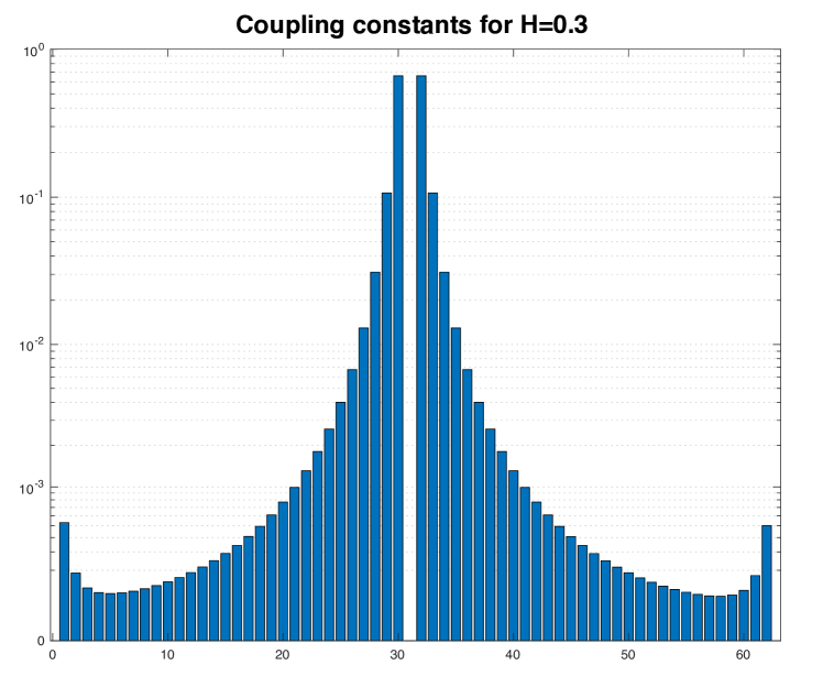
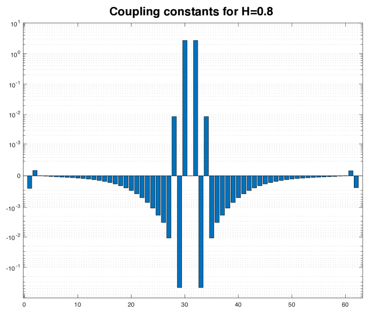
Figure 1: Coupling constants for small Hurst index and large Hurst index [BBS18].

3.2 A non-Gaussian generalization

In general, for the non Gaussian case, the energy function will no more be quadratic. To keep things simple let us for the moment just look at the case of $N=2$.

3.2.1 Energy function for $2$ particle interaction

We look at the increment $Y_{kl}=B^{\beta,\alpha}(k)-B^{\beta,\alpha}(l)$ for $0<l<k<\infty$. The function $H^{\beta,\alpha}(y)=-\ln\big{(}\varrho^{\beta,\alpha}(y)\big{)}$ can be computed from the characteristic function of $Y_{kl}$, i.e., for any $\lambda\in\mathbb{R}^{d}$ we have

$$\mathbb{E}\left(e^{i(B^{\beta,\alpha}(k)-B^{\beta,\alpha}(l),\lambda)}\right) =E_{\beta}\left(-\frac{1}{2}|\lambda|^{2}|k-l|^{\alpha}\right)$$

$$=\int_{\mathbb{R}^{d}}\varrho_{1}^{\beta,\alpha}(y)\exp\big{(}i(y,\lambda)\big{)}dy$$

through the inverse Fourier transform with $\zeta:=|k-l|^{\alpha}$

$$\varrho_{1}^{\beta,\alpha}(y) =\frac{1}{(2\pi)^{d}}\int_{\mathbb{R}^{d}}\exp\big{(}-i(y,\lambda)_{\mathbb{R}^{d}}\big{)}E_{\beta}\left(-\frac{1}{2}|\lambda|^{2}\zeta\right)d\lambda$$

$$=\frac{1}{(2\pi)^{d}}\int_{0}^{\infty}M_{\beta}(\tau)\int_{\mathbb{R}^{d}}\exp\left(-i(y,\lambda)_{\mathbb{R}^{d}}-\frac{1}{2}|\lambda|^{2}\zeta\tau\right)d\lambda\,d\tau.$$

Computing the Gaussian integral and using equality (9) yields

$$\varrho_{1}^{\beta,\alpha}(y) =\frac{1}{(2\pi)^{\nicefrac{{d}}{{2}}}}\int_{0}^{\infty}\frac{1}{(\tau\zeta)^{\nicefrac{{d}}{{2}}}}\exp\left(-\frac{1}{2\tau\zeta}|y|^{2}\right)M_{\beta}(\tau)\,d\tau$$

$$=2^{\nicefrac{{d}}{{2}}}\int_{0}^{\infty}\frac{1}{(4\pi\tau)^{\nicefrac{{d}}{{2}}}}\exp\left(-\frac{1}{4\tau}|\sqrt{2}y|^{2}\right)\big{(}\zeta^{\frac{1}{\beta}}\big{)}^{-\beta}M_{\beta}\big{(}\tau\big{(}\zeta^{\frac{1}{\beta}}\big{)}^{-\beta}\big{)}\,d\tau$$

$$=2^{\nicefrac{{d}}{{2}}-1}\mathbb{M}_{\nicefrac{{\beta}}{{2}}}^{d}\left(\sqrt{2}y,\zeta^{\frac{1}{\beta}}\right).$$

Therefore, up to a constant the function $H^{\beta,\alpha}$ is given by

$$H^{\beta,\alpha}(y)=-\ln\big{(}\mathbb{M}_{\nicefrac{{\beta}}{{2}}}^{d}\big{(}\sqrt{2}y,\zeta^{\frac{1}{\beta}}\big{)}\big{)},\quad y\in\mathbb{R}^{d}.$$

In Figure 2 we plot $H^{\beta,\alpha}$ for different values of $\beta$ and $\alpha$ assuming a time length $|k-l|=1$.

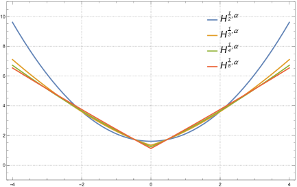
Figure 2: Energy functions $H^{\beta,\alpha}$ for $d=1$; $|k-l|=1$ and $\beta=1,\frac{2}{3},\frac{1}{2},\frac{1}{4}$.

3.2.2 Energy function for $N+1$ particle integration

In general, for an arbitrary $N\in\mathbb{N}$, $H^{\beta,\alpha}$ may be computed using the same technique, namely consider the vectors

$$Y(k):=Y^{\beta,\alpha}(k):=B^{\beta,\alpha}(k)-B^{\beta,\alpha}(k-1),\quad k=1,\ldots,N.$$

and compute the characteristic function of $Y=\big{(}Y^{\beta,\alpha}(1),\ldots,Y^{\beta,\alpha}(N)\big{)}$ for any $\lambda=(\lambda_{1},\ldots,\lambda_{N})\in(\mathbb{R}^{d})^{N}$

$$\mathbb{E}\left(e^{i(Y,\lambda)_{\mathbb{R}^{dN}}}\right)=E_{\beta}\left(-\frac{1}{2}(\lambda,Q\lambda)_{\mathbb{R}^{dN}}\right),$$

where $Q:=Q^{\beta,\alpha}=(a_{kn})_{k,n=1}^{N}$ is the covariance matrix of $Y$ given by

$$a_{kn}=\mathbb{E}\big{(}(Y(k),Y(n))\big{)}=\frac{d}{2\Gamma(\beta+1)}\big{[}|k-1-n|^{\alpha}+|n-1-k|^{\alpha}-2|k-n|^{\alpha}\big{]}.$$

By Proposition (2.9)-2 the density of $Y$ is given by

$$\varrho_{N}^{\beta,\alpha}(y)=\frac{1}{(2\pi)^{\nicefrac{{dN}}{{2}}}\big{(}\det Q\big{)}^{\nicefrac{{d}}{{2}}}}\int_{0}^{\infty}\frac{1}{\tau^{\nicefrac{{dN}}{{2}}}}\exp\left(-\frac{1}{2\tau}\|y\|_{Q}^{2}\right)M_{\beta}(\tau)\,d\tau.$$

Hence, the energy function is

$$H^{\beta,\alpha}(y)=-\ln\left(\varrho_{N}^{\beta,\alpha}(y)\right).$$

Example 3.3.

Let us consider the special case of the 3-particle interaction in dimension $d=1$. The previous result gives the energy function

$$\varrho_{3}^{\beta,\alpha}(y)=\frac{1}{(2\pi)^{d}\big{(}\det Q\big{)}^{\nicefrac{{d}}{{2}}}}\int_{0}^{\infty}\frac{1}{\tau^{d}}\exp\left(-\frac{1}{2\tau}\|y\|_{Q}^{2}\right)M_{\beta}(\tau)\,d\tau.$$

For special values of the parameter $\beta$, we may compute in a closed form the density $\varrho_{3}^{\beta,\alpha}$ as follows.

	$M_{\beta}(\tau)$	$\varrho_{3}^{\beta,\alpha}(y)$
$\beta=0$	$e^{-\tau}$	${\displaystyle\frac{1}{\pi\det(Q)^{\nicefrac{{1}}{{2}}}}K_{0}\left(\sqrt{2}\|y\|_{Q}\right)}$
$\beta=\frac{1}{3}$	${\displaystyle 3^{\nicefrac{{2}}{{3}}}\mathrm{Ai}(3^{-\nicefrac{{1}}{{3}}}\tau)}$	${\displaystyle\frac{1}{8\pi^{3}\det(Q)^{\nicefrac{{1}}{{2}}}}G_{5,0}^{0,0}\left(\frac{\|y\|_{Q}^{6}}{5832}\bigg{|}\;\begin{smallmatrix}\hline\cr\\ \\ 0,0,\frac{1}{3},\frac{1}{3},\frac{2}{3}\end{smallmatrix}\;\right)}$
$\beta=\frac{1}{2}$	${\displaystyle\frac{1}{\sqrt{\pi}}e^{-\frac{\tau^{2}}{4}}}$	${\displaystyle\frac{1}{(2\pi)^{2}\det(Q)^{\nicefrac{{1}}{{2}}}}G_{3,0}^{0,0}\left(\frac{\|y\|_{Q}^{4}}{64}\bigg{|}\;\begin{smallmatrix}\hline\cr\\ \\ 0,0,\frac{1}{2}\end{smallmatrix}\;\right)}$
$\beta=1$	$\delta_{1}(\tau)$	${\displaystyle\frac{1}{2\pi\det(Q)^{\nicefrac{{1}}{{2}}}}\exp\left(-\frac{1}{2}\|y\|_{Q}^{2}\right)}$

Here $K_{\nu}$, $G_{p,q}^{m,n}$ and $\mathrm{Ai}$ are the BesselK, Meijer $G$ and Airy functions respectively, see [OLBC10].

The specific form of the higher order interactions which arise for $\beta<1$, based on a Taylor expansion of $\ln(\varrho^{\beta,\alpha}(y)$ will be the subject of a separated investigation.

Acknowledgement

Financial support from FCT – Fundação para a Ciência e a Tecnologia through the project UID/MAT/04674/2013 (CIMA Universidade da Madeira) is gratefully acknowledged.

References

- [BBS18] W. Bock, J. Bornales, and L. Streit. The dynamics of fractional polymer conformation. In preparation, 2018.
- [BC95] P. Biswas and J. Cherayil. Dynamics of fractional Brownian walks. J. Phys. Chem., 99:816–821, 1995.
- [BK95] Y. M. Berezansky and Y. G. Kondratiev. Spectral Methods in Infinite-Dimensional Analysis, volume 1. Kluwer Academic Publishers, Dordrecht, 1995.
- [DJ72] C. DOMB and G. S. JOYCE. Cluster Expansion for a Polymer Chain. J. Phys. C, 5(9):956–976, 1972.
- [Edw65] S. F. Edwards. The statistical mechanics of polymers with excluded volume. Proc. Phys. Soc., 85:613–624, 1965.
- [GJ16] M. Grothaus and F. Jahnert. Mittag-Leffler Analysis II: Application to the fractional heat equation. J. Funct. Anal., 270(7):2732–2768, April 2016.
- [GJRS15] M. Grothaus, F. Jahnert, F. Riemann, and J. L. Silva. Mittag-Leffler Analysis I: Construction and characterization. J. Funct. Anal., 268(7):1876–1903, April 2015.
- [HKPS93] T. Hida, H.-H. Kuo, J. Potthoff, and L. Streit. White Noise. An Infinite Dimensional Calculus. Kluwer Academic Publishers, Dordrecht, 1993.
- [KST06] A. A. Kilbas, H. M. Srivastava, and J. J. Trujillo. Theory and Applications of Fractional Differential Equations, volume 204 of North-Holland Mathematics Studies. Elsevier Science B.V., Amsterdam, 2006.
- [ML03] G. M. Mittag-Leffler. Sur la nouvelle fonction . CR Acad. Sci. Paris, 137(2):554–558, 1903.
- [ML04] G. M. Mittag-Leffler. Sopra la funzione . Rend. Accad. Lincei, 5(13):3–5, 1904.
- [ML05] G. M. Mittag-Leffler. Sur la représentation analytique d’une branche uniforme d’une fonction monogène. Acta Math., 29(1):101–181, 1905.
- [MP08] A. Mura and G. Pagnini. Characterizations and simulations of a class of stochastic processes to model anomalous diffusion. J. Phys. A: Math. Theor., 41(28):285003, 22, 2008.
- [MP15] A. Mentrelli and G. Pagnini. Front propagation in anomalous diffusive media governed by time-fractional diffusion. J. Comput. Phys., 293:427–441, 2015.
- [MPG03] F. Mainardi, G. Pagnini, and R. Gorenflo. Mellin transform and subordination laws in fractional diffusion processes. Fract. Calc. Appl. Anal., 6(4):441–459, 2003.
- [OLBC10] F. W. J. Olver, D. W. Lozier, R. F. Boisvert, and C. W. Clark. NIST Handbook of Mathematical Functions. Cambridge University Press, 2010.
- [Pol48] H. Pollard. The completely monotonic character of the Mittag-Leffler function . Bull. Amer. Math. Soc., 54:1115–1116, 1948.
- [Sch90] W. R. Schneider. Grey noise. In S. Albeverio, G. Casati, U. Cattaneo, D. Merlini, and R. Moresi, editors, Stochastic Processes, Physics and Geometry, pages 676–681. World Scientific Publishing, Teaneck, NJ, 1990.
- [Sch92] W. R. Schneider. Grey noise. In S. Albeverio, J. E. Fenstad, H. Holden, and T. Lindstrøm, editors, Ideas and Methods in Mathematical Analysis, Stochastics, and Applications (Oslo, 1988), pages 261–282. Cambridge Univ. Press, Cambridge, 1992.
- [SKM93] S. G. Samko, A. A. Kilbas, and O. I. Marichev. Fractional integrals and derivatives. Gordon and Breach Science Publishers, Yverdon, 1993. Theory and applications, Edited and with a foreword by S. M. Nikol’skiĭ, Translated from the 1987 Russian original, Revised by the authors.
- [Wes80] M. J. Westwater. On Edwards’ model for long polymer chains. Comm. Math. Phys., 72(2):131–174, 1980.