DESY 18-119, DO-TH 18/16
Two-mass three-loop effects in deep-inelastic scattering

Abstract:

We report on recent results on the two-mass corrections for massive operator matrix elements at 2- and 3-loop orders in QCD. These corrections form the building blocks of the variable flavor number scheme. Due to the similar values of the charm and bottom quark masses the two-mass corrections form an important contribution.

1 Introduction

The heavy flavor corrections to deep-inelastic scattering to 3-loop order are an important asset to describe the structure functions in the region of lower values of $x$ and to account for the scaling violations correctly, which are different in the massless and massive cases. They are required in precision measurements of the strong coupling constant [1], the determination of the heavy quark masses [2, 3, 4], and the parton distribution functions [5, 4, 6]. In a long program, cf. [7], the different heavy flavor contributions to deep-inelastic scattering are calculated in the region $Q^{2}\gg m^{2}$. For all quantities a series of Mellin moments has been obtained in [8]. The corrections in terms of the general Mellin variable $N$ in the single heavy mass case were calculated in the non-singlet, the pure singlet, the $gq$- and $gg$-cases [9, 10, 11, 12, 13, 14, 15, 16], as well as for all logarithmic corrections [17]. Likewise, we have also obtained all 3-loop anomalous dimensions $\gamma_{ij}$ contributing to the heavy flavor case in Refs. [9, 10, 14, 18], which are the terms $\propto T_{F}$. In case of $\gamma_{qq}^{\rm PS}$ and $\gamma_{qg}$ these are the complete anomalous dimensions. All the 1st order factorizing contributions to the operator matrix element OME $A_{Qg}^{(3)}$, i.e. the contributions due to iterative integrals, have been computed [7]. The calculation of these quantities required the development of several new computation techniques and algorithms, cf. Ref. [19] for a survey.

Already at 2-loop order, two-mass corrections contribute to the heavy flavor Wilson coefficients in the form of reducible terms, cf. [20]. However, for many years, they were not considered in the variable flavor number scheme (VFNS) [21]. At 3-loop order, genuine two-mass contributions appear [20]. For them a number of moments has been calculated expanding in the mass ratio $\eta=m_{c}^{2}/m_{b}^{2}\sim 1/10$, cf. Ref. [22, 23, 20]. In the flavor non-singlet, transversity and $gq$-cases, the general $N$- and $x$-results have been calculated in Ref. [20].

More recently, the complete 3-loop corrections in the flavor pure-singlet case [24] and for the massive OME $A_{gg}$ [25] have been computed. These results are discussed in Section 2. At 2-loop order all two-mass terms are known. In Section 3 we discuss the variable flavor number scheme at 2-loop order, extended to the 2-mass case and describe the corresponding changes for the parton densities [26]. They turn out to be of relevance for precision measurements at the LHC, comparing to the single mass case. Section 4 contains the conclusions.

2 Three-Loop Corrections

Recently we computed the two-mass 3-loop corrections to the OMEs $A_{Qq}^{PS,\rm(3)}$ and $A_{gg,Q}^{\rm(3)}$ in Refs. [24, 25]. Contrary to the 3-loop non-singlet cases and $A_{gq}$, the $\eta$-dependence does not factorize here. The analytic results can be represented in terms of iterated integrals over general alphabets and specific integrals thereof. The iterated integrals are given by

$$G_{f_{0},f_{1},...,f_{k}}(x)=\int_{0}^{x}dyf_{0}(y)G_{f_{1},...,f_{k}}(y),~{}~{}~{}G_{\emptyset}=1,$$ (1)

with letters $f_{l}(x)$, which may depend on the additional parameter $\eta$ and usually form root valued irrational functions. The package HarmonicSums [27, 28, 29] allows the automated calculation of these integrals and the reduction of special constants which appear in this context.

It turns out that the calculation of the OME $A_{Qq}^{PS,\rm(3)}$ cannot be easily done in $N$ space. It is therefore computed in $x$-space and written in terms of a Mellin transform, separating a series of $N$-dependent pre-factors, which will be dealt with at a later stage. The contributing mass ratios are either ruled by $\eta$ or $1/\eta$. In the former case only one principle integration region is obtained, while in the latter case the regions $x\in\{[0,\eta_{-}],[\eta_{-},\eta_{+}],[\eta_{+},1]\}$ contribute, with $\eta_{\pm}=(1\pm\sqrt{1-\eta})/2.$ Besides the letters of the usual harmonic polylogarithms (HPLs) [30], two more letters

$$\sqrt{(4-x)x},~{}~{}~{}~{}~{}~{}\frac{\sqrt{1-4x}}{x}$$ (2)

contribute to the integrals of the Mellin transforms. Finally, one has to incorporate the $N$-dependent pre-factors by partial integration. From the global Mellin-transform one then obtains the two-mass contribution to the OME $A_{Qq}^{PS,\rm(3)}$. The structure of the constant term in $\varepsilon$ is given by

$$a_{Qq}^{PS,\rm(3)}(N) = \int_{0}^{1}dx\,\,x^{N-1}\biggl{\{}K(\eta,x)+\big{(}\theta(\eta_{-}-x)+\theta(x-\eta_{+})\big{)}x\,g_{0}(\eta,x)$$ (3)

$$+\theta(\eta_{+}-x)\theta(x-\eta_{-})\biggl{[}x\,f_{0}(\eta,x)-{\int_{\eta_{-}}^{x}dy}\left(f_{1}(\eta,y)+\frac{y}{x}f_{2}(\eta,y)+\frac{x}{y}f_{3}(\eta,y)\right)\biggr{]}$$

$$+\theta(\eta_{-}-x){\int_{x}^{\eta_{-}}dy}\left(g_{1}(\eta,y)+\frac{y}{x}g_{2}(\eta,y)+\frac{x}{y}g_{3}(\eta,y)\right)$$

$$-\theta(x-\eta_{+}){\int_{\eta_{+}}^{x}dy}\left(g_{1}(\eta,y)+\frac{y}{x}g_{2}(\eta,y)+\frac{x}{y}g_{3}(\eta,y)\right)$$

$$+x\,h_{0}(\eta,x)+{\int_{x}^{1}dy}\left(h_{1}(\eta,y)+\frac{y}{x}h_{2}(\eta,y)+\frac{x}{y}h_{3}(\eta,y)\right)$$

$$+\theta(\eta_{+}-x){\int_{\eta_{-}}^{\eta_{+}}dy}\left(f_{1}(\eta,y)+\frac{y}{\eta_{+}x}f_{2}(\eta,y)+\eta_{+}\frac{x}{y}f_{3}(\eta,y)\right)$$

$$+{\int_{\eta_{+}}^{1}}dy\left(g_{1}(\eta,y)+\frac{y}{x}g_{2}(\eta,y)+\frac{x}{y}g_{3}(\eta,y)\right)\biggr{\}}.$$

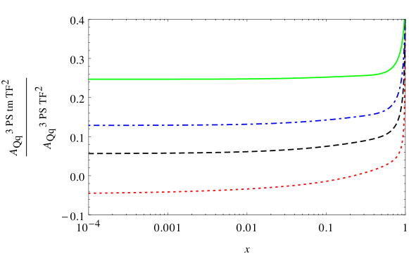
Figure 1: The ratio of the 2-mass (tm) contributions to the massive OME $A_{Qq}^{{\sf PS},(3)}$ to all contributions to $A_{Qq}^{{\sf PS},(3)}$ of $O(T_{F}^{2})$ as a function of $x$ and $\mu^{2}$. Dotted line (red): $\mu^{2}=30~{}\mathrm{GeV}^{2}$. Dashed line (black): $\mu^{2}=50~{}\mathrm{GeV}^{2}$. Dash-dotted line (blue): $\mu^{2}=100~{}\mathrm{GeV}^{2}$. Full line (green): $\mu^{2}=1000~{}\mathrm{GeV}^{2}$. Here the on-shell heavy quark masses $m_{c}=1.59~{}\mathrm{GeV}$ and $m_{b}=4.78~{}\mathrm{GeV}$ [2, 31] have been used; from Ref. [24].

The functions $K,f_{i},g_{i}$ and $h_{i}$ are given in Ref. [24] and can be represented in terms of HPLs at more involved arguments for which the numerical representation is available [32, 33]. In Figure 2 the ratio of the 3-loop two-mass corrections in the pure singlet case is compared to the complete $O(T_{F}^{2}C_{F}(C_{A}))$. The ratio behaves about flat as a function of $x$, with some rise towards $x=1$ and grows with $\mu^{2}$ to typical values of $\sim 0.4$ and is therefore a significant contribution at this order.

In Ref. [25] we have calculated the 3-loop two-mass contributions to the OME $A_{gg}$. Here the calculation can be either performed in $N$- or $x$-space. In $N$-space it requires one analytic Mellin-Barnes integral aside of integrals which can be performed using simpler methods. We have chosen the direct calculation of all contributions, which leads to a large set of individual sum expressions. The largest diagram led to a representation of $\sim 100$MB. We use modern summation technologies [34] encoded in the package Sigma [35, 36]. The sums are first crunched to a few master sums using the package SumProduction. The latter sums are solved individually using EvaluatMultiSums [37] and limits to infinity are performed using built-in routines of HarmonicSums. Finally the results are reduced to basic sums. In the case of the largest diagram, $\sim 78$ days were needed to perform the sums and $\sim 33$ days to reduce to the basis, i.e. to eliminate all relations between the sums. The full summation of this OME took about five months.

Typical sums occurring are

$$S_{\vec{k}}\left(\frac{\eta-1}{\eta},1,N\right),~{}~{}~{}\binom{2N}{N}\sum_{i=1}^{N}\frac{4^{i}\left(\frac{\eta}{\eta-1}\right)^{i}}{i\binom{2i}{i}}S_{\vec{k}}\left(\frac{\eta-1}{\eta},1,i\right),~{}~{}~{}{\rm etc.}$$ (4)

These are generalized harmonic sums at real weights, cf. e.g. [28] and nested binomial sums over these objects, which generalize the class of sums having been dealt with in Ref. [38] before.

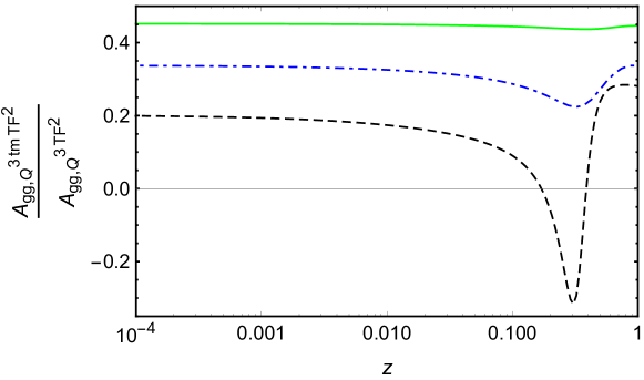
Figure 2: The ratio of the two-mass (tm) contributions to the massive OME $A_{gg,Q}^{(3)\rm{tm}}$ to all contributions to $A_{gg,Q}^{(3)}$ of $O(T_{F}^{2})$ as a function of $z$ and $\mu^{2}$. Dashed line (black): $\mu^{2}=50~{}\mathrm{GeV}^{2}$. Dash-dotted line (blue): $\mu^{2}=100~{}\mathrm{GeV}^{2}$. Full line (green): $\mu^{2}=1000~{}\mathrm{GeV}^{2}$. Here the on-shell heavy quark masses $m_{c}=1.59~{}\mathrm{GeV}$ and $m_{b}=4.78~{}\mathrm{GeV}$ [2, 31] have been used; from Ref. [25].

HarmonicSums provides algorithms to perform the inverse Mellin transform to $x$ space. Here iterated integrals of the kind (1) occur. The letters of the corresponding alphabet are those of the usual HPLs and

$$\sqrt{x(1-x)},~{}~{}\frac{1}{x+\eta(1-x)},~{}~{}\frac{1}{1-x(1-\eta)},~{}~{}\frac{1}{\eta+x(1-\eta)},~{}~{}$$

$$\hskip 28.45274pt\frac{\sqrt{x(1-x)}}{1-x(1-\eta)},~{}~{}\frac{\sqrt{x(1-x)}}{x-\eta(1-x)},~{}~{}\frac{\sqrt{x(1-x)}}{\eta+x(1-\eta)}.$$ (5)

Again rational pre-factors in $N$ have to be absorbed like in the pure singlet case. This leads to a one-dimensional integral representation over integrands out of HPLs with involved argument, well suited for a fast numerical evaluation. In Ref. [25] detailed lists of integrals and special constants of the type (1) emerging in the present context have also been given which can be used in similar calculations.

The relative effect of the 3-loop two-mass contributions to $A_{gg}$ in comparison to all $O(T_{F}^{2}C_{F}$ $(C_{A}))$ terms is illustrated in dependence of $x$ and $\mu^{2}$. The ratio behaves flat in the small $x$ region, with some structure towards larger values of $x$. The ratio grows with $\mu^{2}$ and reaches values of $\sim 0.4$ at $\mu^{2}=1000\mathrm{GeV}^{2}$.

3 Two-mass Corrections in the Variable Flavor Number Scheme

Since the mass ratio squared $\eta$ for charm and bottom is not a very small number, one cannot treat charm quarks as massless at the scale $\mu=m_{b}$. The decoupling in the variable flavor number scheme has therefore to account for the 2-mass effects from $O(\alpha_{s}^{2})$ onward. In the usual VFNS, one decouples one heavy quark at a time, cf. Ref. [21]. Its generalization, cf. Ref. [26], accounts for the two-mass effects. The corresponding transition rules are:

$$f_{{\sf NS},i}(N_{F}+2,\mu^{2}) = \Biggl{\{}1+a_{s}^{2}(\mu^{2})\left[A_{qq,Q}^{{\sf NS},(2,c)}+A_{qq,Q}^{{\sf NS},(2,b)}\right]\Biggr{\}}f_{{\sf NS},i}(N_{F},\mu^{2}),$$ (6)

$$\Sigma(N_{F}+2,\mu^{2}) = \Biggl{\{}1+a_{s}^{2}(\mu^{2})\Bigl{[}A_{qq,Q}^{{\sf NS},(2,c)}+A_{qq,Q}^{{\sf PS},(2,c)}+A_{qq,Q}^{{\sf NS},(2,b)}+A_{qq,Q}^{{\sf PS},(2,b)}\Bigr{]}\Biggr{\}}\Sigma(N_{F},\mu^{2})$$

$$+\Biggl{\{}a_{s}(\mu^{2})\Bigl{[}A_{Qg}^{(1,c)}+A_{Qg}^{(1,b)}\Bigr{]}+a_{s}^{2}(\mu^{2})\Bigl{[}A_{Qg}^{(2,c)}+A_{Qg}^{(2,b)}+A_{Qg}^{(2,cb)}\Bigr{]}\Biggr{\}}G(N_{F},\mu^{2}),$$

$$G(N_{F}+2,\mu^{2}) = \Biggl{\{}1+a_{s}(\mu^{2})\Bigl{[}A_{gg,Q}^{(1,c)}+A_{gg,Q}^{(1,b)}\Bigr{]}+a_{s}^{2}(\mu^{2})\Bigl{[}A_{gg,Q}^{(2,c)}+A_{gg,Q}^{(2,b)}+A_{gg,Q}^{(2,cb)}\Bigr{]}\Biggr{\}}G(N_{F},\mu^{2})$$ (10)

$$+a_{s}^{2}(\mu^{2})\Bigl{[}A_{gq,Q}^{(2,c)}+A_{gq,Q}^{(2,b)}\Bigr{]}\Sigma(N_{F},\mu^{2}),$$

$$\Bigl{[}f_{c}+f_{\bar{c}}\Bigr{]}(N_{F}+2,\mu^{2})=a_{s}^{2}(\mu^{2})A_{Qq}^{{\sf PS},(2,c)}\Sigma(N_{F},\mu^{2})$$

$$~{}~{}~{}~{}~{}~{}+\Biggl{\{}a_{s}(\mu^{2})A_{Qg}^{(1,c)}+a_{s}^{2}(\mu^{2})\Bigl{[}A_{Qg}^{(2,c)}+\frac{1}{2}A_{Qg}^{(2,cb)}\Bigr{]}\Biggr{\}}G(N_{F},\mu^{2}),$$

$$\Bigl{[}f_{b}+f_{\bar{b}}\Bigr{]}(N_{F}+2,\mu^{2})=a_{s}^{2}(\mu^{2})A_{Qq}^{{\sf PS},(2,b)}\Sigma(N_{F},\mu^{2})$$

$$~{}~{}~{}~{}~{}~{}+\Biggl{\{}a_{s}(\mu^{2})A_{Qg}^{(1,b)}+a_{s}^{2}(\mu^{2})\Bigl{[}A_{Qg}^{(2,b)}+\frac{1}{2}A_{Qg}^{(2,cb)}\Bigr{]}\Biggr{\}}G(N_{F},\mu^{2})~{},$$

where $a_{s}=\alpha_{s}/(4\pi)$.

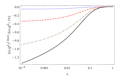
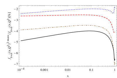
Figure 3: The ratio of the two-mass contribution to the singlet distribution and the complete singlet distribution at $O(a_{s}^{2})$, Eq. (3), in %, as a function of $x$ and $Q^{2}$, using the parton distribution functions [4] and $m_{c}=1.59~{}\mathrm{GeV}$ [2], $m_{b}=4.78~{}\mathrm{GeV}$ [31]. Dotted line: $Q^{2}=30~{}\mathrm{GeV}^{2}$; dashed line: $Q^{2}=100~{}\mathrm{GeV}^{2}$; dash-dotted line: $Q^{2}=1000~{}\mathrm{GeV}^{2}$; full line: $Q^{2}=10000~{}\mathrm{GeV}^{2}$; from Ref. [26].

Comparing the two-mass contributions to the different parton distribution functions with the complete result one finds $O(1\%)$ effects e.g. for the flavor singlet distribution. For the bottom quark distribution the effect can reach $O(5\%)$ at typical scales $Q^{2}\in[30,10000]\mathrm{GeV}^{2}$ at the LHC, see Figure 3.

At 3-loop order still the two-mass corrections to the OME $A_{Qg}^{(3)}$ have to be calculated in order to describe the generalized VFNS. This is work in progress and currently $O(500)$ even moments have been calculated, expanding in the mass ratio $\eta$ to the 5th order.

4 Conclusions

The 2-mass contributions to the massive OMEs in deep-inelastic scattering have a significant numerical effect on a series of parton distributions in precision data analysis. Already at 2-loop order the bottom quark distribution at the LHC receives about 5% corrections, while those for other PDFs are smaller, but not negligible at the 1% level. We have by now calculated all two-mass contributions at 3-loop order, but those for the massive OME $A_{Qg}$. In the latter case, iterative integrals will not be sufficient to represent this quantity and at least iterated integrals over elliptic integrals are contributing as well, cf. [39, 40]. In an ongoing study we investigate first a large number of Mellin moments expanding in the mass ratio $\eta$ working towards a two-mass generalization of the VFNS also at 3-loop order. Along with the present calculations, again new powerful analytic integration techniques have been designed, which can be used in other 2- and 3-loop calculations facing two-scale problems.

Acknowledgment.  This work was supported in part by the Austrian Science Fund (FWF) grant SFB F50 (F5009-N15).

References

-
[1]
S. Bethke et al.,
Workshop on Precision Measurements of alphas,
arXiv:1110.0016 [hep-ph];
S. Moch, S. Weinzierl et al., High precision fundamental constants at the TeV scale, arXiv:1405.4781 [hep-ph];
S. Alekhin, J. Blümlein and S.O. Moch, Mod. Phys. Lett. A 31 (2016) no.25, 1630023. - [2] S. Alekhin, J. Blümlein, K. Daum, K. Lipka and S. Moch, Phys. Lett. B 720 (2013) 172 [arXiv:1212.2355 [hep-ph]].
- [3] A. Gizhko et al., Phys. Lett. B 775 (2017) 233 [arXiv:1705.08863 [hep-ph]].
- [4] S. Alekhin, J. Blümlein, S. Moch and R. Placakyte, Phys. Rev. D 96 (2017) no.1, 014011 [arXiv:1701.05838 [hep-ph]].
- [5] A. Accardi et al., Eur. Phys. J. C 76 (2016) no.8, 471 [arXiv:1603.08906 [hep-ph]].
- [6] S. Alekhin, J. Blümlein and S. Moch, Eur. Phys. J. C 78 (2018) no.6, 477 [arXiv:1803.07537 [hep-ph]].
- [7] J. Blümlein, J. Ablinger, A. Behring, A. De Freitas, A. von Manteuffel, C. Schneider and C. Schneider, PoS (QCDEV2017) 031 [arXiv:1711.07957 [hep-ph]].
-
[8]
I. Bierenbaum, J. Blümlein and S. Klein,
Nucl. Phys. B 820 (2009) 417
[arXiv:0904.3563 [hep-ph]];
J. Blümlein, S. Klein and B. Tödtli, Phys. Rev. D 80 (2009) 094010 [arXiv:0909.1547 [hep-ph]]. - [9] J. Ablinger, J. Blümlein, S. Klein, C. Schneider and F. Wißbrock, Nucl. Phys. B 844 (2011) 26 [arXiv:1008.3347 [hep-ph]].
- [10] J. Ablinger, A. Behring, J. Blümlein, A. De Freitas, A. Hasselhuhn, A. von Manteuffel, M. Round, C. Schneider, and F. Wißbrock, Nucl. Phys. B 886 (2014) 733 [arXiv:1406.4654 [hep-ph]].
- [11] A. Behring, J. Blümlein, A. De Freitas, A. von Manteuffel and C. Schneider, Nucl. Phys. B 897 (2015) 612 [arXiv:1504.08217 [hep-ph]].
- [12] A. Behring, J. Blümlein, A. De Freitas, A. Hasselhuhn, A. von Manteuffel and C. Schneider, Phys. Rev. D 92 (2015) no.11, 114005 [arXiv:1508.01449 [hep-ph]].
- [13] A. Behring, J. Blümlein, G. Falcioni, A. De Freitas, A. von Manteuffel and C. Schneider, Phys. Rev. D 94 (2016) no.11, 114006 [arXiv:1609.06255 [hep-ph]].
- [14] J. Ablinger, A. Behring, J. Blümlein, A. De Freitas, A. von Manteuffel and C. Schneider, Nucl. Phys. B 890 (2014) 48 [arXiv:1409.1135 [hep-ph]].
- [15] J. Ablinger, J. Blümlein, A. De Freitas, A. Hasselhuhn, A. von Manteuffel, M. Round, C. Schneider and F. Wißbrock, Nucl. Phys. B 882 (2014) 263 [arXiv:1402.0359 [hep-ph]].
- [16] J. Ablinger, A. Behring, J. Blümlein, A. De Freitas, A. von Manteuffel, and C. Schneider, DESY 15–112.
- [17] A. Behring, I. Bierenbaum, J. Blümlein, A. De Freitas, S. Klein and F. Wißbrock, Eur. Phys. J. C 74 (2014) no.9, 3033 [arXiv:1403.6356 [hep-ph]].
- [18] J. Ablinger, A. Behring, J. Blümlein, A. De Freitas, A. von Manteuffel and C. Schneider, Nucl. Phys. B 922 (2017) 1 [arXiv:1705.01508 [hep-ph]].
- [19] J. Blümlein and C. Schneider, Int. J. Mod. Phys. A 33 (2018) no.17, 1830015.
- [20] J. Ablinger, J. Blümlein, A. De Freitas, A. Hasselhuhn, C. Schneider and F. Wißbrock, Nucl. Phys. B 921 (2017) 585 [arXiv:1705.07030 [hep-ph]].
- [21] M. Buza, Y. Matiounine, J. Smith and W. L. van Neerven, Eur. Phys. J. C 1 (1998) 301 [hep-ph/9612398].
- [22] J. Ablinger, J. Blümlein, S. Klein, C. Schneider and F. Wißbrock, arXiv:1106.5937 [hep-ph].
-
[23]
J. Ablinger, J. Blümlein, A. Hasselhuhn, S. Klein, C. Schneider and F. Wißbrock,
PoS (RADCOR2011) 031 [arXiv:1202.2700 [hep-ph]]. - [24] J. Ablinger, J. Blümlein, A. De Freitas, C. Schneider and K. Schönwald, Nucl. Phys. B 927 (2018) 339 [arXiv:1711.06717 [hep-ph]].
- [25] J. Ablinger, J. Blümlein, A. De Freitas, A. Goedicke, C. Schneider and K. Schönwald, Nucl. Phys. B 932 (2018) 129 [arXiv:1804.02226 [hep-ph]].
- [26] J. Blümlein, A. De Freitas, C. Schneider and K. Schönwald, Phys. Lett. B 782 (2018) 362 [arXiv:1804.03129 [hep-ph]].
-
[27]
J. Ablinger,
PoS (LL2014) 019;
Computer Algebra Algorithms for Special Functions in Particle Physics, Ph.D.
Thesis, J. Kepler University
Linz, 2012,
arXiv:1305.0687 [math-ph];
A Computer Algebra Toolbox for Harmonic Sums Related to Particle Physics, Diploma Thesis, J. Kepler University Linz, 2009, arXiv:1011.1176 [math-ph];
J. Ablinger, J. Blümlein and C. Schneider, J. Math. Phys. 52 (2011) 102301 [arXiv:1105.6063 [math-ph]];
J. Ablinger, PoS (RADCOR2017) 001. -
[28]
J. Ablinger, J. Blümlein and C. Schneider,
J. Math. Phys. 54 (2013) 082301
[arXiv:1302.0378 [math-ph]];
- [29] J. Ablinger, An improved Algorithm to compute Inverse Mellin Transforms of Nested Binomial Sums, PoS (LL2018) 063.
- [30] E. Remiddi and J.A.M. Vermaseren, Int. J. Mod. Phys. A 15 (2000) 725 [hep-ph/9905237].
- [31] K. A. Olive et al. [Particle Data Group], Chin. Phys. C 38 (2014) 090001.
- [32] T. Gehrmann and E. Remiddi, Comput. Phys. Commun. 141 (2001) 296 [hep-ph/0107173].
- [33] J. Ablinger, J. Blümlein, M. Round and C. Schneider, PoS (RADCOR2017) 010 [arXiv:1712.08541 [hep-th]].
-
[34]
M. Karr, J. ACM 28 (1981) 305;
M. Bronstein, J. Symbolic Comput. 29 (2000), no. 6 841;
C. Schneider, Symbolic Summation in Difference Fields, Ph.D. Thesis RISC, Johannes Kepler University, Linz technical report 01–17 (2001); An. Univ. Timisoara Ser. Mat.-Inform. 42 (2004) 163; J. Differ. Equations Appl. 11 (2005) 799; Appl. Algebra Engrg. Comm. Comput. 16 (2005) 1; J. Algebra Appl. 6 (2007) 415. Motives, Quantum Field Theory, and Pseudodifferential Operators, Clay Mathematics Proceedings Vol. 12, eds. A. Carey, D. Ellwood, S. Paycha and S. Rosenberg, (Amer. Math. Soc) (2010), 285, [arXiv:0904.2323]; Ann. Comb. 14 (2010) 533 [arXiv:0808.2596];
C. Schneider, in: Computer Algebra and Polynomials, Applications of Algebra and Number Theory, J. Gutierrez, J. Schicho, M. Weimann (ed.), Lecture Notes in Computer Science (LNCS) 8942 (2015), 157; [arXiv:1307.7887 [cs.SC]]; J. Symbolic Comput. 43 (2008) 611 [arXiv:0808.2543]; J. Symb. Comput. 72 (2016) 82 [arXiv:1408.2776 [cs.SC]];
J. Symb. Comput. 80 (2017) 616 [arXiv:1603.04285 [cs.SC]]. - [35] C. Schneider, Sém. Lothar. Combin. 56 (2007) 1, article B56b.
- [36] C. Schneider, Computer Algebra in Quantum Field Theory: Integration, Summation and Special Functions Texts and Monographs in Symbolic Computation eds. C. Schneider and J. Blümlein (Springer, Wien, 2013) 325, arXiv:1304.4134 [cs.SC].
-
[37]
J. Ablinger, J. Blümlein, S. Klein and C. Schneider,
Nucl. Phys. Proc. Suppl. 205-206 (2010) 110
[arXiv:1006.4797 [math-ph]];
J. Blümlein, A. Hasselhuhn and C. Schneider, PoS (RADCOR 2011) 032 [arXiv:1202.4303 [math-ph]];
C. Schneider, J. Phys. Conf. Ser. 523 (2014) 012037 [arXiv:1310.0160 [cs.SC]]. - [38] J. Ablinger, J. Blümlein, C.G. Raab and C. Schneider, J. Math. Phys. 55 (2014) 112301 [arXiv:1407.1822 [hep-th]].
- [39] J. Ablinger, J. Blümlein, A. De Freitas, M. van Hoeij, E. Imamoglu, C. G. Raab, C.-S. Radu and C. Schneider, J. Math. Phys. 59 (2018) no.6, 062305 [arXiv:1706.01299 [hep-th]].
- [40] J. Blümlein, A. De Freitas, M. van Hoeij, E. Imamoglu, P. Marquard and C. Schneider, PoS (LL2018) 017 [arXiv:1807.05287 [hep-ph]].