Schwarzschild dynamical model of the Fornax dwarf spheroidal galaxy

Abstract

We present a full dynamical model of the Fornax dwarf spheroidal galaxy obtained with the spherically symmetric Schwarzschild orbit superposition method applied to the largest kinematic data set presently available. We modelled the total mass content of the dwarf with the mass-to-light ratio $\Upsilon$ varying with radius and found that Fornax is with high probability embedded in a massive and extended dark matter halo. We estimated the total mass contained within 1 kpc to be $M(<1\,$kpc$)=1.25^{+0.06}_{-0.13}\times 10^{8}\,$M_☉. The data are consistent with the constant mass-to-light ratio, i.e. the mass-follows-light model, only at 3$\sigma$ level, but still require a high value of $\Upsilon\approx 11.2\,$M${}_{\sun}/$L_☉. Our results are in general agreement with previous estimates of the dynamical mass profile of Fornax. As the Schwarzschild method does not require any assumptions on the orbital anisotropy of the stars, we obtained a profile of the anisotropy parameter $\beta$ as an output of our modelling. The derived anisotropy is close to zero in the centre of the galaxy and decreases with radius, but remains consistent with isotropic orbits at all radii at 1$\sigma$ confidence level.

1 Introduction

The distribution of mass in galaxies remains a subject of lively debate between astrophysicists supporting the existence of dark matter and those favouring various implementations of modified gravity. The most significant discrepancies between the mass profiles inferred from kinematics of the tracer and the distribution of light, which in this paper we will interpret as indications of high dark matter content, are found in galaxies belonging to the class referred to as dwarf spheroidals (dSph). Thanks to their proximity, dSphs of the Local Group (LG) are the focus of attention in studies of dark matter distribution. Resolving single stars, both in photometric and spectroscopic observations, gives astronomers a unique opportunity to model these galaxies in detail, which at the moment seems to be limited mainly by the relatively small numbers of measurements.

The most numerous data samples, both photometric and spectroscopic, are currently available for the Fornax dSph, the second largest and most luminous (after the Sagittarius dSph) satellite of the Milky Way. As a result, over the last two decades the dynamics of Fornax has been modelled by many authors using various methods. The simplest approach takes advantage of estimators of dynamical mass roughly independent of the velocity anisotropy of the tracer, measured at the half-light radius (or another predefined scale; Walker et al. 2007; Walker et al. 2009b; Walker & Peñarrubia 2011; Amorisco et al. 2013). Interestingly, Walker & Peñarrubia (2011) and Amorisco et al. (2013) identified multiple stellar populations of different metallicities as well as spatial distribution and kinematics which allowed them to measure the mass at various radii.

More sophisticated methods aim to reproduce the full mass profile of the galaxy. The most widely used modelling based on solving Jeans equations (Binney & Tremaine, 2008) suffers from the mass-anisotropy degeneracy (Binney & Mamon, 1982) and therefore requires additional assumptions concerning the anisotropy (e.g. constant with radius or of particular functional form) and/or mass profiles (e.g. mass follows light, a particular density profile of the dark matter halo). The Fornax dwarf has been modelled with various combinations of assumptions by Łokas (2002), Wang et al. (2005), Klimentowski et al. (2007), (Strigari et al.2008), Łokas (2009), Hayashi & Chiba (2012), Hayashi & Chiba (2015), (Diakogiannis et al.2017) and Read et al. (2018). We can also find in the literature phase-space (Amorisco & Evans, 2011) and action-based (Pascale et al., 2018) models as well as those applying the Schwarzschild (Schwarzschild, 1979) orbit superposition method (Breddels & Helmi, 2013; Jardel & Gebhardt, 2012; Jardel & Gebhardt, 2013).

To give just an order of magnitude, the dynamical mass within the half-light radius of 0.71 kpc (at the adopted distance of 147 kpc) is estimated to be $5.6\times 10^{7}$M_☉ (McConnachie, 2012), with the mass-to-light ratio $\sim 10$M_☉/L_☉, which suggests that Fornax is embedded in a massive dark matter halo. The galaxy is also elongated: the projected ellipticity $\epsilon=1-b_{p}/a_{p}=0.30\pm 0.01$, where $b_{p}$ and $a_{p}$ are the projected semi-minor and semi-major axis, respectively (Irwin & Hatzidimitriou, 1995). It shows traces of a major merger about 6 Gyr ago (, del Pino et al.2015) and probably did not interact strongly with the Milky Way due to its extended orbit (Battaglia et al., 2015) so has no strong tidal features and can be assumed to be in dynamical equilibrium. Additionally, the galaxy contains little to no gas (, Bouchard et al.2006), which may appear surprising in the light of the above since a most likely mechanism to strip the gas, namely the ram pressure, would require at least one close approach to the Milky Way.

Although the observations of LG dwarfs evince their non-negligible ellipticities (Mateo, 1998; McConnachie, 2012), most studies still treat them as spherically symmetric. We can find in the literature only a few attempts of generalizing shapes of galaxies for various purposes. These studies include: full dynamical modelling (Jardel & Gebhardt 2012; Jardel & Gebhardt 2013; Jardel et al. 2013 assuming axisymmetric edge-on stellar component and spherical dark matter halo; Hayashi & Chiba 2012; Hayashi & Chiba 2015 assuming both components to be axisymmetric), calculations of corrections to possible dark matter annihilation fluxes (Sanders et al. 2016 obtaining values of mass with strong assumption or from estimators) or tracing the evolution of a satellite (Sanders et al. 2018 using predefined density profiles). Unfortunately, up to date there has been no research done on mock objects showing that the intrinsic shapes and therefore multiple free parameters (up to 6 for Hayashi & Chiba 2015) can be reliably derived with currently available data samples.

In this paper we present a new full dynamical model of the Fornax dwarf obtained using the spherically symmetric Schwarzschild orbit superposition method in the form developed in Kowalczyk et al. (2017, 2018). In Kowalczyk et al. (2018) we used mock data selected from the outcome of an $N$-body simulation of a major merger of two disky dwarf galaxies that led to the formation of a dark matter dominated, spheroidal galaxy similar to Fornax. We examined the effect of its non-spherical shape on the inferred properties and quantified the systematic errors inherent in the method. The results of this previous study and the similarities between the mock object and the real Fornax will help us interpret the outcome of the present work.

The paper is organized as follows. In Section 2 we present the properties of Fornax and our observational data sets whereas in Section 3 and 4 we describe the modelling procedures and the obtained results. In Section 5 we summarize our findings and extensively compare them to those available in the literature.

2 Data

In this section we give a general overview of our observational data samples, both photometric and spectroscopic. The detailed description of the measurements and procedures used in merging various catalogues can be found in (del Pino et al.2015) and (del Pino et al.2017). In Table 1 we present the observational parameters of Fornax which we assume in this paper: the coordinates of the centre, the distance and relative velocity with respect to the observer and the total luminosity. For consistency with the data sets which will be described in the next subsections we use the values given in (del Pino et al.2013) and references therein.

Table 1: Observational parameters of the Fornax dSph (del Pino et al.2013 and references therein).

quantity	value
RA $\alpha$ (J2000.0)	2h$\,39\arcmin\,53.1\arcsec$
Dec $\delta$ (J2000.0)	$-34^{\circ}\,30\arcmin\,16.0\arcsec$
heliocentric distance [kpc]	136 $\pm$ 5
heliocentric velocity [km  s-1]	55.3 $\pm$ 0.1
luminosity $L_{V}\,[$L${}_{\sun}]$	$1.55\times 10^{7}$

2.1 Photometry

Our photometric sample is an extensive ensemble of archival data with more than $3.5\times 10^{5}$ stars reaching V$\sim$23.5 with the completeness of 50% based on the calibrated photometry obtained by Stetson (2000), Stetson (2005) and (de Boer et al.2012). It covers the main body of the galaxy extending up to more than $\sim 1.2^{\circ}$ to the north-east from the centre. In order to ensure that all stellar magnitudes are in the same photometric system, a very precise internal calibration between the catalogues was applied. This calibration was performed using the best measured stars common between the catalogues (18.5 < V < 23.5), by an iterative second-order fitting between their sky coordinates, magnitudes and colour. After the calibration, the catalogues were merged, keeping all the non-common stars between the catalogues as well as only the best-measured magnitudes for the common ones. Finally, we cleaned our photometry from probable non-stellar objects and stars with high magnitude errors by using quality flags provided by Daophot and Dophot. A detailed description of the whole procedure together with the assumed acceptable ranges for the quality flags can be found in (del Pino et al.2015).

As shown by (del Pino et al.2015), the spatial distributions of stars belonging to different stellar populations differ significantly. Therefore, we decided to limit the sample used for the derivation of the luminosity profile to stars of the red giant branch (RGB), the horizontal branch (HB) and the red clump (RC) as the spectroscopy is usually done for these types of objects. In order to guarantee high (90%) completeness of our sample we considered only stars with V<22, additionally excluding the stars: of the main sequence, strongly reddened (on the right-hand side of the RGB) and brighter than RGB and HB. The selected sample contained 65 797 stars and for simplicity we will refer to them as RGB.

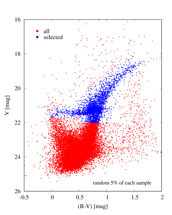
Figure 1: Colour-magnitude diagram for the stars in the Fornax dwarf spheroidal. In red we present random 5% of all available stars with photometric measurements and in blue 5% of the stars selected for the luminosity profile (RGB, HB, RC).

We present the comparison of the full sample (in red) and the stars chosen for the measurement of the luminosity profile (in blue) in the colour-magnitude diagram of Figure 1. To avoid overcrowding only random 5% of each sample is shown.

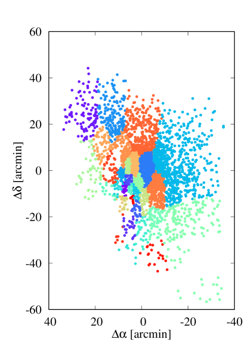
Figure 2: The last iteration of the Voronoi tessellation for the stars with line-of-sight velocities. Each dot represents a star and colours denote different Voronoi cells.

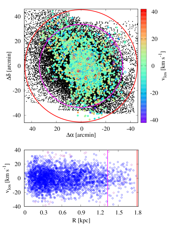
Figure 3: Top panel: Two-dimensional map of the Fornax dSph. Small black dots represent the sample of stars chosen for the luminosity profile. With large dots we overplot the kinematic data colour-coded with the line-of-sight velocity corrected for the bulk movement of the galaxy as a whole. Diamonds show stars rejected as a result of the Voronoi tessellation. With coloured circles (and vertical lines in the bottom panel) we present the outer radii chosen for the data sets used in modelling: luminosity profile (magenta) and moments of the line-of-sight velocity (red). Bottom panel: Line-of-sight velocity measurements as a function of distance from the centre of the galaxy. Blue circles represent stars used in the modelling whereas pink diamonds show stars rejected by the Voronoi tessellation.

2.2 Spectroscopy

The spectroscopic list of stars was obtained after combining the catalogues with the largest number of spectroscopic measurements for RGB stars in Fornax (Battaglia et al., 2006; Walker et al., 2009a; Kirby et al., 2010; Letarte et al., 2010). The procedure followed to combine all catalogues is explained in detail in (del Pino et al.2017). For the present work only good precision in the line-of-sight velocity of the stars was required which allowed us to include some of the Fornax stars with poorly determined chemistry but reliable kinematic measurements. Some of the stars were common to two or more catalogues and in such cases we adopted the weighted mean of all the measurements (with weights determined by the errors) for the line-of-sight velocity of the star.

The resulting spectroscopic list was cleaned from outliers and doubtful member stars with the Voronoi tessellation technique. Using this method, an adaptive grid is set over the stellar coordinates, adjusting the sizes of the cells to keep a constant number of stars within each cell. Consequently, areas with lower number of observed stars are covered with larger grid cells. The tessellation was performed in an iterative way until convergence, keeping $\sim$80 stars per cell in each iteration and removing from every cell stars lying outside the 3$\sigma$ of the line-of-sight velocity distribution within the cell. In Figure 2 we present the last iteration of the Voronoi cleaning. Dots represent the total of 3 286 stars kept as highly probable members of Fornax and are colour-coded according to the cell to which they were assigned.

We note that some of the cells end up with less stars than our target number of 80 stars. This is due to the lack of sampled stars in the boundaries of the cells that causes the process of tessellation to stop before reaching the desired number of stars. This does not cause any problem when considering individual cells since 10 or more stars is sufficient for screening out clear contaminants.

2.3 Final data set

In Figure 3 we present the final data set which we will use for the modelling in Section 3. The top panel shows a two dimensional map of the sky centred on the coordinates given in Table 1. Small black dots denote all RGB stars described in Section 2.1 whereas large dots represent the stars with spectroscopic measurements, colour-coded with the line-of-sight velocity relative to the mean velocity of Fornax (Section 2.2). Circles indicate the outer boundaries of the luminosity profile (magenta) and kinematic data (red). We will justify the selection of those boundaries in Section 3.

The kinematic data (line-of-sight velocities) as a function of the physical distance from the centre of Fornax are presented in the bottom panel of Figure 3 with blue circles. In both panels we show the stars rejected during the Voronoi cleaning with diamonds.

3 Modelling

In this section we describe the modelling procedures applied in order to derive the density and anisotropy profiles of the Fornax dSph. In the top panel of Figure 4 we present the luminosity profile of Fornax in terms of stellar density where points indicate the measurements from the data described in Section 2.1 while the solid line shows the best-fitting Sérsic profile (Sérsic, 1968) given as:

$$n_{\star}(R)=n_{0}\,{\rm exp}[-(R/R_{\rm s})^{1/m}],$$ (1)

where $n_{0}$ is the normalization, $R_{\rm s}$ is the characteristic radius and $m$ is the Sérsic index. The parameters of the best-fitting profile are: $n_{0}=6.951\times 10^{4}$ kpc^-2, $R_{\rm s}=0.454$ kpc, $m=0.808$ and they are also cited in the figure. As the uncertainties of our dynamical modelling (see Sec. 4) will be driven mostly by the sampling errors of kinematics, we will assume that the fit is very precise and will not include errors associated with it in further analysis.

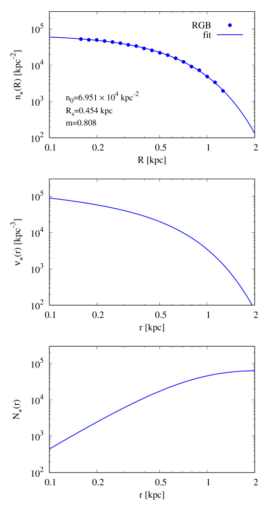
Figure 4: Top panel: The luminosity profile of the Fornax dSph. Blue dots represent the measurements based on the RGB stars whereas the line shows the best-fitting Sérsic profile. The parameters of the fit are quoted in the bottom left corner. Middle and bottom panels: The 3D deprojected density and cumulative stellar number profiles assuming the parameters of the best-fitting Sérsic distribution.

The inner radius of the profile, i.e. the radial distance of the innermost data point, was set to $r=0.16$ kpc in order to avoid overcrowding, i.e. the artificial underestimation of values due to the insufficient spatial resolution of an instrument, while for the outer radius we adopted $r=1.26$ kpc, the maximum value of the radius of the circle with full coverage by data fields (see Figure 3).

We obtained the 3D stellar density $\nu_{\star}(r)$ and the cumulative stellar number profiles $N_{\star}(r)$ by deprojecting the best-fitting Sérsic profile with the analytical formulae (, Lima, Gerbal & Márquez1999) and we present them in the middle and bottom panels of Figure 4, respectively. The total number of stars resulting from the fit is $N_{\rm s}$=65 235.3.

We modelled the data by applying the spherically symmetric Schwarzschild orbit superposition method which we have adopted for dwarf spheroidals of the Local Group and tested on mock data in Kowalczyk et al. (2017) and Kowalczyk et al. (2018). As in previous studies we used 10 bins linearly spaced in radius and set the outer radius to $r=1.8$ kpc. Such a value was a compromise between using all velocity measurements not rejected by the cleaning procedure (see Section 2.2) and having a reasonable number of stars in the outermost bin in order to maintain satisfying statistics.

We quantify the projected distribution of stellar mass in Fornax as a fraction of mass in a given bin $M_{l}(R)$ under the assumption of equal masses of stars. The fraction of stellar mass was calculated as a ratio between the number of stars in a bin and the total number derived from the parameters of the best-fitting Sérsic profile. Since the luminosity profile is extrapolated for small ($r<0.16$ kpc) and large ($r>1.26$ kpc) radii, fractions in the innermost and two outermost bins were obtained ‘theoretically’, i.e. estimating the number of stars by integrating the fitted profile. Moreover, the kinematics of the data set was expressed in terms of proper moments of the line-of-sight velocity: the second ($m_{2}$), third ($m_{3}$) and fourth ($m_{4}$), calculated with estimators based on the sample of $N$ line-of-sight velocity measurements $v_{i}$ (Łokas & Mamon, 2003).

The profiles of the fraction of mass and line-of-sight velocity moments are presented in the consecutive panels of Figure 5 where the error bars denote the sampling errors. For the fraction of mass we adopted Poissonian errors (which in Figure 5 are smaller than the data points) whereas the errors for the line-of-sight velocity moments were calculated analytically assuming normal parent distributions (Kendall & Stuart, 1977).

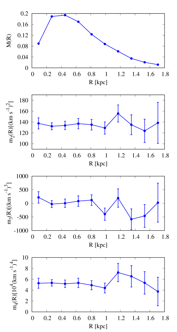
Figure 5: Projected mass fraction and the 2nd, 3rd and 4th velocity moment (in consecutive panels) of the Fornax dSph calculated in 10 radial bins. Error bars represent 1$\sigma$ sampling errors.

We modelled the total mass distribution in Fornax with the local mass-to-light ratio:

$$\Upsilon(r)=\frac{\nu_{\rm tot}(r)}{{\nu}_{\star}(r)},$$ (2)

varying with radius from the centre of the galaxy following a cubic function in log-log scale:

$$\log\Upsilon(r)=\left\{\begin{array}[]{ll}\log\Upsilon_{0}&\rm{for}\,\,\,r<r_{0}\\ a(\log r-\log r_{0})^{3}+\log\Upsilon_{0}&\rm{for}\,\,\,r>r_{0}\\ \end{array}\right.$$ (3)

where $\Upsilon(r)$ is dimensionless and $r$ is given in kpc. Such a function has been first introduced by Kowalczyk et al. (2018) as a satisfactory approximation of the true profile derived for their mock Fornax dSph analogue when limiting the fitting to two free parameters, $a$ and $\Upsilon_{0}$, which are constants defining the density model. We assume that in the centre the mass-to-light ratio is constant, i.e. that mass follows light as the derivation of the central slope is rather impossible with the current data. We set the minimum of the cubic curve to $\log r_{0}=-0.8$ as a consequence of the adopted value of the innermost datapoint for the luminosity profile.

In order to express $\Upsilon_{0}$ in the convenient units of the solar mass-to-light ratio we assumed that the whole stellar mass in Fornax is distributed in the same way as our RGB sample and translated the total luminosity (Table 1) to the total stellar mass with $\Upsilon_{\star}=1$ M${}_{\sun}/$L_☉. Therefore, $\Upsilon_{0}$ denotes the excess of mass in the centre of the galaxy.

For the purpose of Schwarzschild modelling we created libraries containing 1200 orbits (100 values of energy in units of the radius of the circular orbit sampled logarithmically and 12 values of the relative angular momentum $l=L/L_{\rm max}$, where $L_{\rm max}$ is the angular momentum of the circular orbit, sampled linearly) with apocentres in the range [0.04 : 3.34] kpc. Orbits were integrated in the gravitational potential generated by the total mass distribution dependent on $a$ and $\Upsilon_{0}$. We used $a\in$ [0 : 2.4] with a step of $\Delta a$=0.05 and $\Upsilon_{0}=1$ whereas other values of $\Upsilon_{0}$ were obtained with a simple algebraic transformation (see Kowalczyk et al. 2018).

We fitted each orbit library to the data by minimizing the objective function $\chi^{2}$ given as:

$$\chi^{2}=\sum_{l}\sum_{n}\Bigg{(}\frac{M_{l}^{\rm obs}m_{n,l}^{\rm obs}-\sum_{k}\gamma_{k}M_{l}^{k}m_{n,l}^{k}}{\Delta(M_{l}^{\rm obs}m_{n,l}^{\rm obs})}\Bigg{)}^{2}$$ (4)

with weights $\gamma_{k}$ imposed on orbits and under the constraints that for each orbit $k$ and each bin $l$:

$$\left\{\begin{array}[]{l}|M_{l}^{\rm obs}-\sum_{k}\gamma_{k}M_{l}^{k}|\leq\Delta M_{l}^{\rm obs}\\ \gamma_{k}\geq 0\\ \sum_{k}\gamma_{k}=1\end{array}\right.$$ (5)

where $M_{l}^{k}$, $M_{l}^{\rm obs}$ are the fractions of the projected mass of the tracer contained within the $l$th bin for the $k$th orbit or from the observations and $m_{n,l}^{k}$, $m_{n,l}^{\rm obs}$ are $n$th proper moments. $\Delta$ denotes the measurement uncertainty associated with a given parameter. The velocity moments were weighted with the projected masses and to derive the errors we treated both quantities as independent. We executed the $\chi^{2}$ fitting with rigid constraints with the non-negative quadratic programming (QP) implemented in the CGAL library (The CGAL Project, 2015).

4 Results

As a result of our Schwarzschild modelling we obtained a map of absolute values of the objective function $\chi^{2}$ as a function of the two parameters of the mass-to-light ratio profile: $a$ and $\Upsilon_{0}$. Similarly to the procedure undertaken in our previous works, we fitted a two-dimensional 8th order ($\sim a^{4}\Upsilon_{0}^{4}$) surface to the map. We derived the minimum of the surface and present the resulting $\Delta\chi^{2}=\chi^{2}-\chi^{2}_{\rm min}$ in Figure 6 with the colour scale. We marked the minimum with a yellow dot and the 1, 2, 3$\sigma$ levels with white curves. As the numerical minimum does not correspond to any model on the adopted grid, we identified the best-fitting mass model as a set of parameters closest to the minimum along the confidence level. It is shown in Figure 6 as a green dot.

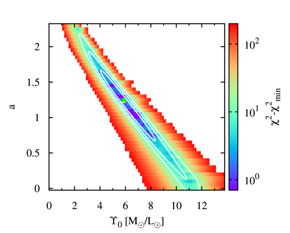
Figure 6: Colour map of absolute values of the objective function $\chi^{2}$ (relative to the global minimum derived from the fitted surface) on the grid of different mass-to-light ratio models. The minimum is marked with the yellow dot whereas the green dot indicates the best-fitting mass profile, i.e. the profile on the grid closest to the global minimum along the contours of equal $\Delta\chi^{2}$ plotted with white curves.

The $\chi^{2}$ map shows that the data favour high values of the curvature parameter $a$, indicating that the excess of mass in Fornax is significantly higher at large radii. It can be explained with the presence of an extended dark matter halo. It is worth pointing out that the mass-follows-light model, i.e. the model assuming that the spatial distribution of the total mass is the same as the distribution of light, which for our parametrization corresponds to $a=0$, is consistent with the data at the 3$\sigma$ confidence level. However, this model requires a high value of the mass-to-light ratio, $\Upsilon_{0}\in$ [10.6 : 11.7]. Since it is significantly higher than stellar mass-to-light ratios estimated for dwarf spheroidals (Mateo, 1998), such a mass-follows-light model also supports the conclusion that Fornax is embedded in a heavy dark matter halo.

The derived best-fitting model and the 1$\sigma$ confidence region allowed us to construct Figure 7 where in consecutive panels we present the profiles of the mass-to-light ratio, the total mass density, the cumulative total mass and the velocity anisotropy. Results for the best-fitting model are presented with a blue solid line whereas the shaded areas denote the spread of values among the density models contained within the 1$\sigma$ region (the innermost elongated ellipse in Figure 6). Black vertical lines mark the inner radius of the luminosity profile and the outer radius of kinematic data from left to right, respectively.

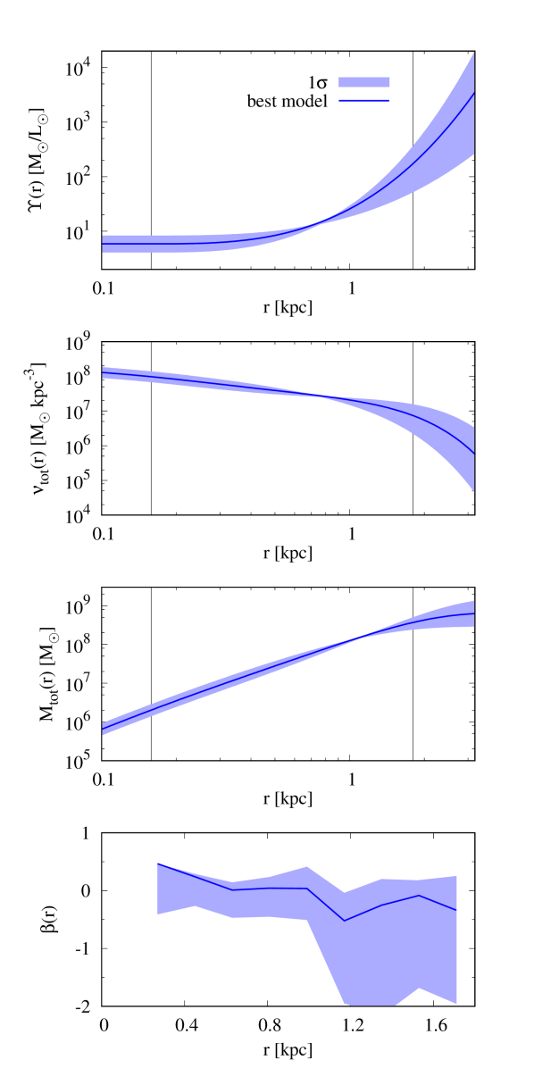
Figure 7: Results of Schwarzschild modelling of the Fornax dSph based on the fitted mass-to-light ratio profiles. In consecutive panels: profiles of the mass-to-light ratio, total density, cumulative total mass and anisotropy. Blue solid lines show the results for the best-fitting mass profile (green dot in Figure  6) whereas shaded regions denote the spread of values for the models from within 1$\sigma$ confidence level. Black vertical lines mark the inner radius of the luminosity profile and the outer radius of the data used in modelling (from left to right, respectively).

We note that the mass profile is derived with remarkably small uncertainties, even at the outskirts of the galaxy and in particular the mass enclosed within the radius of 1 kpc is determined very precisely. This scale is not accidental as Wolf et al. (2010) identified the existence of a radius (dependent on the light profile of an object) at which the enclosed mass is almost independent of the velocity anisotropy. A rough estimate of this radius for the Fornax luminosity distribution gives a value close to 1 kpc (see appendix B in Wolf et al. 2010).

The anisotropy profile is constrained with much lower accuracy, especially at larger distances where the 1$\sigma$ confidence region is rather wide. The profile derived for the best-fitting mass model is decreasing with radius, slightly radial ($\beta>0$) in the centre and tangential ($\beta<0$) at larger radii. However, the mean value is close to isotropic, $\bar{\beta}=-0.04$.

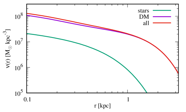
Figure 8: A comparison of density profiles of stars (in green), dark matter (in purple) and total mass (in red) for the best-fitting mass-to-light ratio model.

In Kowalczyk et al. (2018) we demonstrated the existence of a systematic bias in the results of our spherically symmetric modelling caused by the elliptical shape of the studied object. We showed that for the observations along the longest axis the derived anisotropy profile was growing, however the values of anisotropy were systematically underestimated with the mean offset of $\sim 0.4$ for the best-fitting model, whereas for the observations along the shortest axis the best-fitting model was consistent with isotropic orbits but the wide 1 $\sigma$ confidence level allowed the anisotropy profile to grow (with the mean minimal offset with respect to the true values $\Delta\beta\approx 0.1$) or decrease with radius. Since the simulated galaxy we used in that work as well as mock data obtained with observations along the shortest axis of the stellar component are similar to Fornax (assuming its prolate shape), we should expect an analogous bias in the present results. Comparing the bottom panels of Figure 7 and figure 8 in Kowalczyk et al. (2018) (where the blue colour denotes the results of interest) we can see that the anisotropy inferred for Fornax is consistent with the real anisotropy profile growing with radius from 0 to 0.5 but biased as a result of spherically symmetric modelling of a spheroidal object observed along the minor axis.

For the sake of completeness and to better illustrate the derived model, in Fig. 8 we also present a comparison of density profiles of stars (in green), dark matter (in purple) and total mass (in red) for the best-fitting mass-to-light ratio model.

5 Summary and discussion

Using the observational data of (del Pino et al.2015) and (del Pino et al.2017) and our version of the Schwarzschild orbit superposition method (Kowalczyk et al., 2017, 2018) we constructed a full dynamical model of the Fornax dSph. We parametrized the mass content with the mass-to-light ratio varying with radius from the centre of the galaxy described by the two parameters formula given by Eq. (3). We obtained the total mass profile and inferred the presence of an extended dark matter halo. We estimated the mass contained within the outer boundary of our kinematic data set to be $M_{\rm tot}(1.8\,$kpc$)=3.7^{+1.4}_{-1.3}\times 10^{8}\,$M_☉.

Additionally, our Schwarzschild approach allowed us to derive the unparametrized velocity anisotropy profile. We obtained nearly isotropic orbits in the centre of the galaxy and mildly tangential ones at the outskirts, however the uncertainties grew strongly with radius.

Despite the complicated chemodynamical structure of Fornax (Walker & Peñarrubia, 2011; Amorisco & Evans, 2012; , del Pino et al.2015, del Pino et al.2017) in this work we applied only one stellar population. While it is our intention to implement multiple populations in our Schwarzschild code in the future, careful tests on mock data are needed in order to maintain satisfying quality of results. Therefore, it is beyond the scope of the present paper. Nevertheless, when deriving the light distribution we limited our photometric sample to stars of the red giant branch, horizontal branch and red clump, to be consistent with the population from which the kinematic data originate.

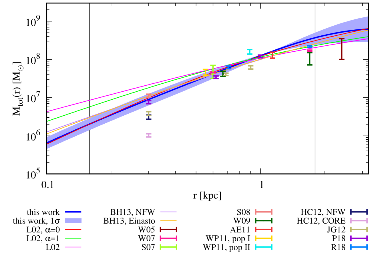
Figure 9: The comparison of derived mass profile (blue line and light blue shaded 1$\sigma$ confidence level) with the profiles (other colour lines) and estimates (error bars) from the literature. For the estimates we present only 1$\sigma$ error bars (without data points) to avoid crowding.
Acronyms used: L02 Łokas (2002), BH13 Breddels & Helmi (2013), W05 Wang et al. (2005), W07 Walker et al. (2007), S07 (Strigari et al.2007), S08 (Strigari et al.2008), W09 Walker et al. (2009b), AE11 Amorisco & Evans (2011), WP11 Walker & Peñarrubia (2011), HC12 Hayashi & Chiba (2012), JG12 Jardel & Gebhardt (2012), P18 Pascale et al. (2018), R18 Read et al. (2018)

In Figure 9 we present an extensive comparison of our estimated mass profile for Fornax with different results from the literature. The blue line and the light blue shaded area represent the profile and the 1$\sigma$ confidence region obtained in this work. For the results from the literature we applied the following approach: 1) if the parameters of the models were given or could be read from the figures, we reproduce full mass profiles, 2) if a full profile was derived but is difficult to reproduce, the values at specific radii given by the authors are presented (for Read et al. 2018 the values of the dark matter mass were read from a figure and we used our values of the stellar mass at given radii to calculate the total masses), 3) values based on estimators are shown at appropriate radii. In order to avoid crowding, in the first case we draw just the profiles with the best-fitting parameters whereas for the other cases we present only 1$\sigma$ error bars (without data points). The references are given in the caption of Figure 9.

Table 2: Comparison of the derived values of anisotropy (both constant and varying with radius).

[b]

$\beta=$ const
			model	$\beta$
Łokas (2002)			$\alpha=0$	$-0.36\pm$0.33
			$\alpha=1$	$-1.5\pm$0.8
			$\alpha=1.5$	$-2.6\pm$1.6
Walker et al. (2007)				$-0.5$
Walker et al. (2009b)				$-0.6$
$\beta(r)$
		shape	$\beta(0.3$ kpc)	$\beta(1.7$ kpc)
this work		decreasing	0.46${}^{+0.00}_{-0.87}$	$-0.34^{+0.59}_{-1.62}$
Hayashi & Chiba (2012)		local max 1	0.09	0.26
Jardel & Gebhardt (2012)	major axis	growing	0.17${}^{+0.19}_{-0.55}$	0.49${}^{+0.16}_{-0.25}$ 2
	minor axis	growing	$-0.38^{+0.27}_{-0.40}$	0.52${}^{+0.09}_{-0.21}$ 2
Breddels & Helmi (2013)		flat	0.2$\pm$0.2
Pascale et al. (2018)		flat	0.05${}^{+0.05}_{-0.05}$	0.1${}^{+0.15}_{-0.20}$
Read et al. (2018)		flat	$-0.26^{+0.16}_{-0.14}$	$-0.18^{+0.08}_{-0.15}$ 3

• $\beta(1$ kpc)=0.32

• Values at the outermost point $r\approx 0.92$ kpc.

• Values at the outermost point $r=1$ kpc.

When considering the full mass profile, our result agrees very well at all radii with the profile derived by Łokas (2002) for the cored model $\alpha=0$, where $\alpha$ denotes the asymptotic central slope for a generalized Navarro-Frenk-White profile (NFW, Navarro et al. 1997) and generally disagrees with models for $\alpha=1,1.5$. This is not surprising since in our modelling we assumed that in the centre the dark matter slope follows that of the stellar component and they have the central slope of 0.32. Cuspy profiles derived by Breddels & Helmi (2013): NFW and Einasto (Einasto, 1965) give very similar mass profiles which lie within our 1$\sigma$ confidence level, but fall a little below our result at radii where our profile has the narrowest confidence region.

Table 3: Comparison of total masses and values of the anisotropy for mass-follows-light models.

[b]

	$M_{\infty}$ [$\times 10^{8}$ M☉]	$\bar{\beta}$	$\beta=$ const
this work	1.74$\pm$0.04	$-1.94^{+0.11}_{-0.03}$ 1
Klimentowski et al. (2007) 2	2.03${}^{+0.38}_{-0.32}$		$-0.17^{+0.37}_{-0.63}$
	1.91${}^{+0.32}_{-0.31}$		$-1.82^{+1.02}_{-2.66}$
Łokas (2009)	1.57$\pm$0.07		$-0.32^{+0.14}_{-0.17}$
(Diakogiannis et al.2017)	$1.613^{+0.050}_{-0.075}$	$-0.95^{+0.78}_{-0.72}$

• Mean weighted with deprojected light profile.

• Rows correspond to different sample cleaning procedures.

Our mass profile is consistent within 1$\sigma$ confidence level with most of the results presented with the error bars. We can distinguish three types of discrepancies: at large radii ($r>1.5$ kpc) as they correspond to outer boundaries of data sets (this work, Wang et al. 2005; Walker et al. 2007; Walker et al. 2009b), with the result for the metal-poor population (pop II) from Walker & Peñarrubia (2011) and with results of axisymmetric models by Hayashi & Chiba (2012) and Jardel & Gebhardt (2012). Whereas the low values obtained by Hayashi & Chiba (2012) can be caused by the assumption of the non-spherical shape of the dark matter halo, the interpretation of systematically lower masses given by Jardel & Gebhardt (2012) is more complicated. In Kowalczyk et al. (2018) we showed that the results for observations of a galaxy along the shortest axis are not biased whereas those for the longest axis are overestimated. Assuming that the orientation of Fornax is between these extreme cases, our profile should be slightly overestimated. On the other hand, values obtained with mass estimators are on average unbiased (Kowalczyk et al., 2013; Campbell et al., 2017) and since they are in good agreement with our profile at various radii, it suggests that bias on our results is rather insignificant. We will return to the results of axisymmetric modelling when comparing the derived anisotropy profiles. Interestingly, our model is in good agreement with the results of Pascale et al. (2018) who partially took into account the ellipticity by assigning to each star a ‘circularized radius’ dependent on both coordinates and the flattening.

In Table 2 we compare the values of the derived anisotropy. The top part of the Table refers to the models with the anisotropy assumed to be constant with radius whereas in the bottom part we present the values for models varying with radius. We show the values at two radii: 0.3 kpc and 1.7 kpc which correspond to the inner and outer radii of our anisotropy profile (see Figure 7). We also indicate the general shape of the profile.

The values of the anisotropy from Walker et al. (2007) and the profiles varying with radius (except for Breddels & Helmi 2013) were read from the figures published in these papers and are therefore approximate. We note that the profiles of mass distribution and anisotropy in Jardel & Gebhardt (2012) are shown as a function of radius given in arcseconds so the outer radius of the anisotropy profile should correspond to about 0.92 kpc (as given in Table 2). However, after careful analysis of the text and given our experience with Fornax, we have reasons to believe that the profiles in Jardel & Gebhardt (2012) are really plotted as a function of the physical radius (in kpc) with the outer boundary of $\sim 1.6$ kpc.

The values of anisotropy assumed to be constant with radius (top part of Table 2) from the literature are consistently negative whereas our mean anisotropy is close to zero. This discrepancy, except for the result in Łokas (2002) for $\alpha=0$, can be explained with the mass-anisotropy degeneracy as the corresponding mass estimates are lower at large radii (see Figure 9). Moreover, despite of deriving full anisotropy profiles, Breddels & Helmi (2013) and Pascale et al. (2018) also obtained flat models but with higher values, closer to ours.

As already stated in Section 4, our derived anisotropy profile is consistent with a growing profile biased by the ellipticity of the galaxy and its observation along the shortest axis. Interestingly, such a growing profile would agree with the findings of Jardel & Gebhardt (2012) (see Table 2) who, contrary to other authors, obtained anisotropy increasing with radius. Instead of spherically symmetric modelling, they applied an axisymmetric approach but assumed a particular orientation of the galaxy, avoiding an additional parameter. Even more general axisymmetric models were applied by Hayashi & Chiba (2012) and the dominant trend in their anisotropy profile is also increasing. It may suggest that their treatment of the elliptical projected shape of the galaxy was able to lift the bias.

Finally, in Table 3 we compare our results for the mass-follows-light model, i.e. with $a=0$, with the total mass and anisotropy estimates for the same type of mass distribution from the literature. Since the light profiles and the total luminosity estimates differ between the studies, we present the derived total masses. All the results are consistent with our findings within 1$\sigma$ confidence level.

Results for the anisotropy are less conclusive. Since our method recovers the full anisotropy profile (instead of just a constant value) we present the range of mean values of the anisotropy. They were calculated by weighting the radius-dependent quantities with the deprojected stellar mass fractions as the values of anisotropy rapidly decrease from $\approx 0$ at the centre to $\approx-7$ at the outer boundary of the data set ($r=1.8$ kpc). The derived profiles are approximately consistent with the results presented by (Diakogiannis et al.2017) who also derive the full anisotropy profile. Similarly to our findings, they obtained the profile decreasing from 0 in the centre to $\approx-1.5$ at 1 kpc. However, their profile has a minimum of $-2$ at 1.5 kpc (which was the outer radius of the data set) and grows beyond. The mean value cited in the Table is as given by (Diakogiannis et al.2017). For the models with constant anisotropy, our result agrees well with the value derived by Klimentowski et al. (2007) for a less restrictive procedure of data sample cleaning but strongly disagrees with their other value and findings of Łokas (2009). We note that the latter two studies used a much more restrictive sample cleaning method than our conservative $3\sigma$ clipping. Nevertheless, all studies reproduce a tangentially biased anisotropy. Since our modelling suggests the existence of an extended dark matter halo, mass-follows-light models underestimate the mass content at large radii and necessarily yield lower, more tangential, values of anisotropy in order to recreate the same velocity distribution with the Jeans equation.

References

- Amorisco & Evans (2011) Amorisco N. C., Evans N. W., 2011, MNRAS, 411, 2118
- Amorisco & Evans (2012) Amorisco N. C., Evans N. W., 2012, ApJ, 756, L2
- Amorisco et al. (2013) Amorisco N. C., Agnello A., Evans N. W., 2013, MNRAS, 429, L89
- Battaglia et al. (2015) Battaglia G., Sollima A., Nipoti C., 2015, MNRAS, 454, 2401
- Battaglia et al. (2006) Battaglia G. et al., 2006, A&A, 459, 423
- Binney & Mamon (1982) Binney J., Mamon G. A., 1982, MNRAS, 200, 361
- Binney & Tremaine (2008) Binney J., Tremaine S., 2008, Galactic Dynamics, 2 edn. Princeton University Press, Princeton, NJ
- (8) Bouchard A., Carignan C., Staveley-Smith L., 2006, AJ, 131, 2913
- Campbell et al. ( 2017) Campbell D. J. R. et al., 2017, MNRAS, 469, 2335
- (10) de Boer T. J. L. et al., 2012, A&A, 544, A73
- Breddels & Helmi (2013) Breddels M. A., Helmi A., 2013, A&A, 558, A35
- (12) del Pino A., Hidalgo S. L., Aparicio A., Gallart C., Carrera R., Monelli M., Buonanno R., Marconi G., 2013, MNRAS, 433, 1505
- (13) del Pino A., Aparicio A., Hidalgo S. L., 2015, MNRAS, 454, 3996
- (14) del Pino A., Aparicio A., Hidalgo S. L., Łokas E. L., 2017, MNRAS, 465, 3708
- (15) Diakogiannis F. I. et al., 2017, MNRAS, 470, 2034
- Einasto (1965) Einasto J., 1965, Trudy Astrofizicheskogo Instituta Alma-Ata, 5, 87
- Hayashi & Chiba (2012) Hayashi K., Chiba M., 2012, ApJ, 755, 145
- Hayashi & Chiba (2015) Hayashi K., Chiba M., 2015, ApJ, 810, 22
- Irwin & Hatzidimitriou (1995) Irwin M., Hatzidimitriou D., 1995, MNRAS, 277, 1354
- Jardel & Gebhardt (2012) Jardel J. R., Gebhardt K., 2012, ApJ, 746, 89
- Jardel & Gebhardt (2013) Jardel J. R., Gebhardt K., 2013, ApJ, 775, L30
- Jardel et al. ( 2013) Jardel J. R., Gebhardt K., Fabricius M. H., Drory N., Williams M. J., 2013, ApJ, 763, 91
- Kirby et al. (2010) Kirby E. N. et al., 2010, ApJS, 191, 352