Self-regulation promotes cooperation in social networks

Abstract

Cooperative behavior in real social dilemmas is often perceived as a phenomenon emerging from norms and punishment. To overcome this paradigm, we highlight the interplay between the influence of social networks on individuals, and the activation of spontaneous self-regulating mechanisms, which may lead them to behave cooperatively, while interacting with others and taking conflicting decisions over time. By extending Evolutionary game theory over networks, we prove that cooperation partially or fully emerges whether self-regulating mechanisms are sufficiently stronger than social pressure. Interestingly, even few cooperative individuals act as catalyzing agents for the cooperation of others, thus activating a recruiting mechanism, eventually driving the whole population to cooperate.

Cooperation in human populations is a fundamental phenomenon, which has fascinated many scientists working in different fields, such as biology, sociology, economics, [1, 2, 3, 4, 5, 6], and, more recently, engineering [7, 8, 9]. Actually, in the analysis of social dilemmas, such as the prisoner’s dilemma game, cooperation is often assumed to be the result of suitable norms [10, 11] and punishment mechanisms [12, 13, 14, 15, 16, 17]. Further approaches claim that cooperation emerges from other factors, such as reputation [18, 19], synergy and discounting [20], social diversity [21] and positive interactions [22].

Mathematical models tackling the problem of cooperation are typically grounded on evolutionary game theory, where a population of individuals taking part in a game repeated over time is considered. Each individual decides to be Cooperative ($C$) or Defective ($D$) when playing one or more two-players games with other individuals. Eventually he obtains a given payoff, and may decide to opt for changing his strategy. In a generic two-players game, $R$ is the reward when both cooperate, $T$ is the temptation to defect when the opponent cooperates, $S$ is the sucker’s payoff earned by a cooperative player when the opponent is a free rider, and $P<R$ is the punishment for mutual defection. The social dilemma arises when the temptation to defect is stronger than the reward for cooperation ($T>R$), and the punishment for defection is preferred to the sucker’s payoff ($P>S$). This scheme is known as prisoner’s dilemma game, and it well describes many real world situations, occuring in fields like environmental protection, biology, psychology, international politics, economics and so on. In all these cases, defectors earn a higher payoff than unconditional cooperators. As a consequence, cooperators are doomed to extinction. This fact has been proven to be true for both the deterministic setting of the replicator equation and for stochastic game dynamics of finite populations, assuming that players are equally likely to interact with each other [23, 24, 25]. Interestingly, a consistent part of the recent literature [26, 27, 28, 29, 30, 31, 32, 33] showed that the networked structure of the population may favor the emergence of cooperation.

In this work, we consider members of a social network. To be realistic, these individuals may choose to be $100\%$ cooperative, $100\%$ defective, as in the standard case, or also fuzzy strategies, such as $50\%-50\%$ cooperative/defective. More interestingly, in this study cooperation is shown to be promoted by spontaneous self-regulating mechanisms, according to the idea that humans seem to have an innate tendency to cooperate with one another even when it goes against their rational self-interest, as pointed out by Vogel in [34]. Specifically, self-regulation is modeled as an inertial term and the resulting effects on the population dynamics are extensively analyzed both theoretically and by means of numerical simulations.

Consider a social network defined as a finite population of players $v=\{1,\ldots,N\}$, arranged on a directed graph described by adjacency matrix ${\bf A}=\{a_{v,w}\}$, where $a_{v,w}=1$ if player $v$ is influenced by player $w$, and $0$ otherwise. The in-degree $k_{v}=\sum_{w=1}^{N}a_{v,w}$ of a player represents the number of neighbors of the generic player $v$. At each time instant a player can choose his own level of cooperation, indicated by $x_{v}\in[0,1]$, to play $k_{v}$ two-persons games with all his neighbors. Notice that $x_{v}=1$ represents full cooperation ($C$), $x_{v}=0$ means full defection ($D$), and $x_{v}\in(0,1)$ stands for a partial level of cooperation. Accordingly, when any two connected players $v$ and $w$ take part in a game, the payoff for $v$ is defined by the continuous function $\phi:[0,1]\times[0,1]\to\mathbb{R}$:

$$\phi(x_{v},x_{w})=[x_{v},1-x_{v}]\begin{bmatrix}R&S\\ T&P\end{bmatrix}\begin{bmatrix}x_{w}\\ 1-x_{w}\end{bmatrix}.$$ (1)

Notice that for $x_{v},x_{w}\in\{0,1\}$, we recover the payoffs $R$, $T$, $S$ and $P$ previously introduced. Player’s $v$ payoff $\phi_{v}$ collected over the network is the sum of all outcomes of two-player games with neighbors. Formally, the payoff function $\phi_{v}:[0,1]^{N}\to\mathbb{R}$ is defined as follows:

$$\phi_{v}({\bf x})=\sum_{w=1}^{N}a_{v,w}\phi(x_{v},x_{w}),$$ (2)

where ${\bf x}=[x_{1},x_{2},\ldots,x_{N}]^{\top}$. Player $v$ is able to appraise whether a change of his strategy $x_{v}$ produces an improvement of his payoff $\phi_{v}$. Indeed, if the derivative of $\phi_{v}$ with respect to $x_{v}$ is positive (negative), the player would like to increase (decrease) his level of cooperation. Of course, when the derivative is null, then the player has no incentive to change his mind. This mechanism is modeled by the EGN equation [35, 36], which reads as follows:

$$\dot{x}_{v}=x_{v}(1-x_{v})\displaystyle\frac{\partial\phi_{v}}{\partial x_{v}},$$ (3)

where the sign of $\dot{x}_{v}$ depends only on the term $\partial\phi_{v}/\partial x_{v}$, since $x_{v}(1-x_{v})\geq 0$. Unlike the standard replicator equation, which deals with the distribution of strategies over a well mixed population, where players are indistinguishable except for their strategies, the EGN is a system of ODEs, each one describing the strategy evolution of the specific player $v$ (when dealing with more than two strategies, the dimension of the ODE system increases accordingly). Following equation (2), the derivative of the payoff $\phi_{v}$ is:

$$\frac{\partial\phi_{v}}{\partial x_{v}}=\sum_{w=1}^{N}a_{v,w}\frac{\partial\phi(x_{v},x_{w})}{\partial x_{v}}.$$

Moreover, from equation (1) we get that:

$$\frac{\partial\phi(x_{v},x_{w})}{\partial x_{v}}=(R-T+P-S)x_{w}-(P-S)=(\sigma_{C}+\sigma_{D})x_{w}-\sigma_{D},$$ (4)

where $\sigma_{C}=R-T$ and $\sigma_{D}=P-S$ [37]. For the specific case of a strict prisoner’s dilemma game, $\sigma_{C}<0$ and $\sigma_{D}>0$. According to [28] and [38], unilateral defection is preferred to mutual cooperation when $\sigma_{C}<0$, while $\sigma_{D}>0$ indicates the preference for mutual defection over unilateral cooperation. When the effect of $\sigma_{C}$ is stronger than $\sigma_{D}$ ($|\sigma_{C}|>\sigma_{D}$), the game is more influenced by temptation (hereafter called T-driven game), while in the other case ($|\sigma_{C}|<\sigma_{D}$) punishment is more effective, and hence the game will be called P-driven. Since $\sigma_{C}<0$ and $\sigma_{D}>0$, we have that $\partial\phi(x_{v},x_{w})/\partial x_{v}\leq 0$ for all $x_{w}\in[0,1]$. Therefore, also $\partial\phi_{v}/\partial x_{v}\leq 0$ and then $\dot{x}_{v}\leq 0,$ showing that the level of cooperation decreases over time towards full defection.

As reported in equation (3), $\partial\phi_{v}/\partial x_{v}$ depends only on the state of neighboring players, not on the current state $x_{v}$ of player $v$ himself. On the contrary, the willingness to pursue cooperation as a greater good follows from internal mechanisms correlated to personal awareness and culture. These mechanisms should act as inertial terms able to reduce the rational temptation to defect, depending on the current strategy $x_{v}$ of player himself. Generally, this aspect is not taken into account in the mathematical modeling, even though it normally characterizes complex individuals like humans [34].

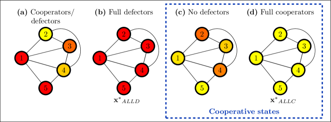
Figure 1: Cooperation distribution over a social network. (a) Coexistence of full cooperators (yellow circles), partial cooperators (orange circles) and full defectors (red circles). (b) Population composed only by full defectors. This state is the $N$-dimensional vector ${\bf x}^{*}_{ALLD}=[0,0,\ldots,0].$ (c) No full defectors are present within the population. (d) Population composed only by full cooperators. This state is the $N$-dimensional vector ${\bf x}^{*}_{ALLC}=[1,1,\ldots,1].$ Configurations reported in (c) and (d) represent cooperative steady states (i.e. $x_{v}>0~{}\forall v$).

To fill this gap, in this paper internal mechanisms are introduced in the EGN equation by adding a term $f_{v}$ balancing $\partial\phi_{v}/\partial x_{v}$. This term is weighted by a parameter $\beta_{v}$ which measures the inertia of a player with respect to his neighbors’ actions [9]. The extended Self-Regulated EGN equation, hereafter called SR-EGN, is reported in Figure 2. Notice that full cooperative ${\bf x}_{ALLC}^{*}=[1,1,\ldots,1]^{\top}$, full defective ${\bf x}_{ALLD}^{*}=[0,0,\ldots,0]^{\top}$, and fuzzy configurations ${\bf x}^{*}=[x_{1}^{*},x_{2}^{*},\ldots,x_{N}^{*}]^{\top}$ with $x_{v}^{*}>0$ for at least one $v$, are steady states of the SR-EGN equation (see Figure 1). Further details on steady states are reported in Appendix A.

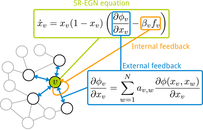
Figure 2: SR-EGN equation. The strategy dynamics of player $v$ (green node) is ruled by the SR-EGN equation (green box). It includes two terms: the external feedback term (blue box) $\partial\phi_{v}/\partial x_{v}$, accounting for the external mechanisms related to game interactions (blue arrows) with the $k_{v}$ neighbors (black nodes), and the internal feedback term (orange box) $\beta_{v}f_{v}$, modeling the self regulating processes of node $v$ (the orange self loop).

Inspired by self-regulation in animal societies [39], the term $\beta_{v}f_{v}$ is modeled as an internal feedback describing a virtual game that each individual plays against himself, i.e. a self game. This game is characterized by the same parameters $\sigma_{C}$ and $\sigma_{D}$ of the two-player games. Therefore, the self-regulating function $f(v)$ is written as:

$$f_{v}=(\sigma_{C}+\sigma_{D})x_{v}-\sigma_{D}.$$ (5)

Notice that $f_{v}$ is similar to equation (4), where $x_{w}$ has been replaced by $x_{v}$, thus conceiving the individual $v$ himself as one of his own “opponents”. “What kind of outcome can I earn if I apply a given strategy to myself?”: a generic player in our model can be aware of the conflicting context where he participates, and he may know the importance of cooperation as a primal objective to be pursued. Remarkably, this term models a spontaneous learning process, thus representing a time varying feature of each individual.

The complete SR-EGN equation studied in this paper can be rewritten as follows:

$$\dot{x}_{v}=\displaystyle x_{v}(1-x_{v})\left[k_{v}\left((\sigma_{C}+\sigma_{D})\bar{x}_{v}-\sigma_{D}\right)-\beta_{v}\left((\sigma_{C}+\sigma_{D})x_{v}-\sigma_{D}\right)\right],$$ (6)

where $\bar{x}_{v}=(1/k_{v})\sum_{w=1}^{N}a_{v,w}x_{w}$ is the average player resulting from the decisions of all neighboring players of $v$. Besides $\sigma_{C}$ and $\sigma_{D}$, the two fundamental parameters of this model are $k_{v}$ and $\beta_{v}$. $k_{v}$ is the in-degree of player $v$, thus accounting for the influence of the network (external feedback) on his decision. The second parameter is the weighting factor $\beta_{v}$ modulating self-regulation. When $\beta_{v}=0$, the individual is somehow “member of the flock”, since his strategy changes only according to the outcome variations of game interactions with neighbors, embodied by $\partial\phi_{v}/\partial x_{v}$. In this case, we recover the standard EGN equation (3), and defection is unavoidable. Positive values of $\beta_{v}$ represent an “aware resistance” of players to the external feedback.

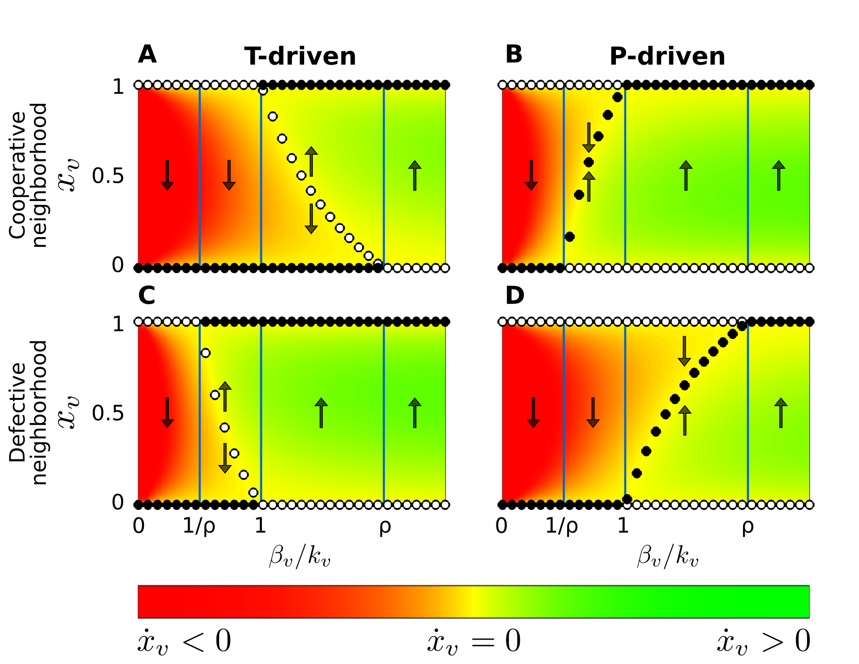
Figure 3: Flow of the SR-EGN equation. Colors represent the value of the derivative $\dot{x}_{v}$ as a function of $x_{v}$ and $\beta_{v}/k_{v}$. Black and white circles correspond to attractive and repulsive steady states for player $v$, respectively. Arrows are used to schematically highlight the direction of the dynamics. The flow for a player $v$ connected only to full cooperators ($\bar{x}_{v}=1$) in T-driven game ($\sigma_{C}=-2$ and $\sigma_{D}=1$) and in P-driven game ($\sigma_{C}=-1$ and $\sigma_{D}=2$) are reported in subplots A and B, respectively. Instead, the case of a player connected only to full defectors ($\bar{x}_{v}=0$) is shown in subplots C (T-driven) and D (P-driven). Vertical blue lines are depicted for $\beta_{v}/k_{v}=1/\rho$, $\beta_{v}/k_{v}=1$ and $\beta_{v}/k_{v}=\rho$. The intermediate steady states corresponding to partial levels of cooperation are always located between $1/\rho$ and $\rho$.

The main result of this paper is that SR-EGN equation can explain the emergence of cooperation in a social network. More specifically, when the awareness is stronger than the level of connectivity of each player, i.e. $\beta_{v}>k_{v}$, then state ${\bf x^{*}}_{ALLC}$ is an attractor for the dynamics of the population, as well as a Nash equilibrium [35] of the complete game, while at the same time total defection ${\bf x^{*}}_{ALLD}$ is repulsive. Furthermore, when

$$\beta_{v}>\rho k_{v},$$ (7)

where $\rho=\left|\sigma_{C}/\sigma_{D}\right|\geq 1$ for a T-driven game and $\rho=\left|\sigma_{D}/\sigma_{C}\right|\geq 1$ for a P-driven game, then ${\bf x^{*}}_{ALLC}$ is a global attractor. In other words, starting from any initial strategy $x_{v}(t=0)>0~{}\forall v$, all players will eventually become full cooperators. These results are formally proved in the Appendix B. Notice that convincing individuals with high degree $k_{v}$ to be cooperative requires potentially large values of $\beta_{v}$. Anyway, in the following we show that cooperation may be also achieved for smaller value of $\beta_{v}$.

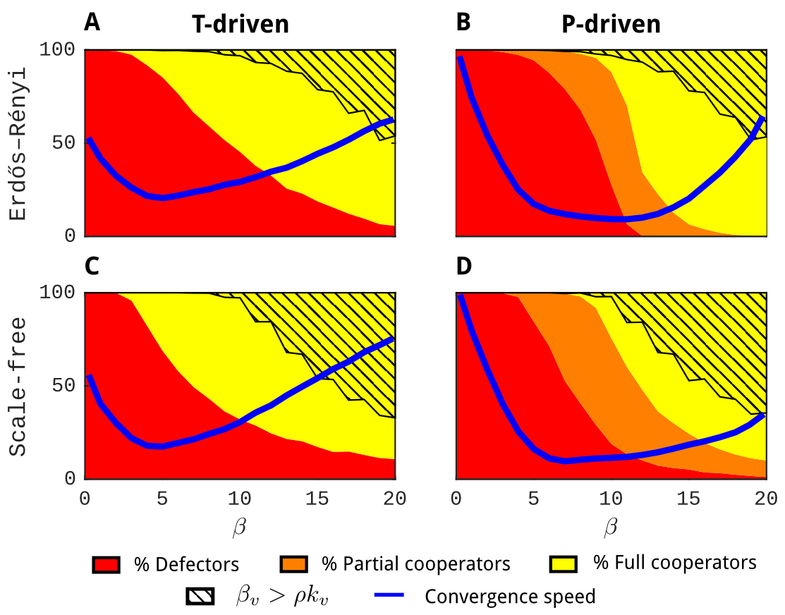
Figure 4: Average distribution of strategies and convergence speed. For different graph topologies (ER and SF), $500$ graphs with $N=100$ nodes and average degree $\bar{k}=10$ are considered. Initial conditions are randomly chosen in the set $(0,1)$. For a T-driven game ($\sigma_{C}=-2$ and $\sigma_{D}=1$) and a P-driven game ($\sigma_{C}=-1$ and $\sigma_{D}=2$), and for different values of the parameter $\beta_{v}=\beta\in\{0,\ldots,20\}~{}\forall v$, the SR-EGN equation is simulated system until a steady state is reached. The average distribution of strategies of the whole population, dividing it into 3 subgroups, is reported: defectors in red ($x_{v}^{*}<10^{-4}$), partial cooperators in orange ($10^{-4}\leq x_{v}^{*}\leq 1-10^{-4}$) and full cooperators in yellow ($x_{v}^{*}>1-10^{-4}$). The hatched area represent the average percentage of population for which the theoretical rule $\beta_{v}>\rho k_{v}$ is satisfied. The superposed blue lines represent the convergence speed, experimentally estimated as the inverse of the time required to the population for reaching the steady state.

In Figure 3 the value of $\dot{x}_{v}$ is reported with colors as a function of $\beta_{v}/k_{v}$ and $x_{v}$, together with the attracting (black circles) and repulsive (white circles) steady states for player $v$. Arrows are used to depict the direction of the dynamics. The derivative $\dot{x}_{v}$ is analyzed for both a cooperative ($\bar{x}_{v}=1$, Figures 3A and 3B) and a defective ($\bar{x}_{v}=0$, Figures 3C and 3D) neighborhood sets. The interesting region of all graphs is $\beta_{v}/k_{v}<\rho$, in which the values of the parameters are below the theoretical threshold (7). In all cases, the smaller is this ratio, the lower is the probability to cooperate, while the higher is the ratio, the higher is the probability to cooperate. For intermediate values ($1/\rho<\beta_{v}/k_{v}<\rho$), the formation of steady states corresponding to partial levels of cooperation is observed. These steady states separate the regions where defection or cooperation dominates. For the T-driven games (Figures 3A and 3C), these new equilibria are repulsive, thus creating bistable dynamics which leads player to cooperate or defect according to their initial conditions. Moreover, the probability to cooperate raises for increasing values of $\beta_{v}$ or decreasing the in-degree. Notice that, since the temptation is prominent for this game, if $\bar{x}_{v}$ moves from $1$ (Figure 3A) to $0$ (Figure 3C), the region of partial steady states exists for lower values of $\beta_{v}/k_{v}$, thus easing cooperation. On the other hand, for P-driven games (Figures 3B and 3D), the fuzzy steady states are attractive, thus ensuring at least a certain level of cooperation also in the intermediate region. Interestingly, since the punishment is strong, the presence of cooperators in the neighborhood facilitates the convergence to a cooperative state. Specifically, if $\bar{x}_{v}$ moves from $1$ (Figure 3B) to $0$ (Figure 3D), the region of partial steady states exists for higher values of $\beta_{v}/k_{v}$, thus preventing cooperation. This phenomenon will be explained better in the following experiments.

Figure 3 shows that, from the single player’s point of view, cooperation is also feasible for values of $\beta_{v}$ below the theoretical threshold (7). For completeness, the behavior of the whole population is studied by means of numerical simulations. We investigate the probability for a population to be cooperative by running $500$ simulations of different random networks (Erdös-Rényi (ER) and Scale-Free (SF)) with $N=100$ and average degree $\bar{k}=10$ (and thus the average in-degree is also $10$). Moreover, all individuals share the same self-regulating factor $\beta_{v}=\beta\in\{0,\ldots,20\}$. This experiment has been repeated for T-driven and P-driven games, using initial conditions randomly generated for each simulation.

In Figure 4 the percentages of full defectors (red area), partial cooperators (orange area) and full cooperators (yellow area) at steady state are reported as a function of $\beta$. The fraction of individuals who satisfy the theorem (7) is highlighted with the hatched pattern. Notice that the number of defectors decreases by increasing $\beta$. Consistently with the results shown in Figure 3, bistable behavior is observed for T-driven game (Figures 4A and 4C), for which the population splits into two groups of full defectors and full cooperators. Partial cooperation (orange area) is present for P-driven game (Figures 4B and 4D). According to the results shown in Figures 3B and 3D, where the presence of cooperative neighborhood fosters cooperation for single players, we observe the same phenomenon in Figures 4B and 4D, extended to the whole population. In particular, the presence of even few cooperators is able to recruit their neighboring players to switch their strategies from defection to cooperation. Increasing $\beta$, these players, together with those satisfying the threshold (7), are able to recruit to cooperation an increasing number of individuals. The average convergence speed of the system to a steady state, reported by blue lines, shows a slowdown of the dynamics for intermediate values of $\beta$. Specifically, this occurs when a small fraction of cooperators appears in the population, until a sufficiently large number of individuals start to cooperate, thus accelerating significantly the dynamics.

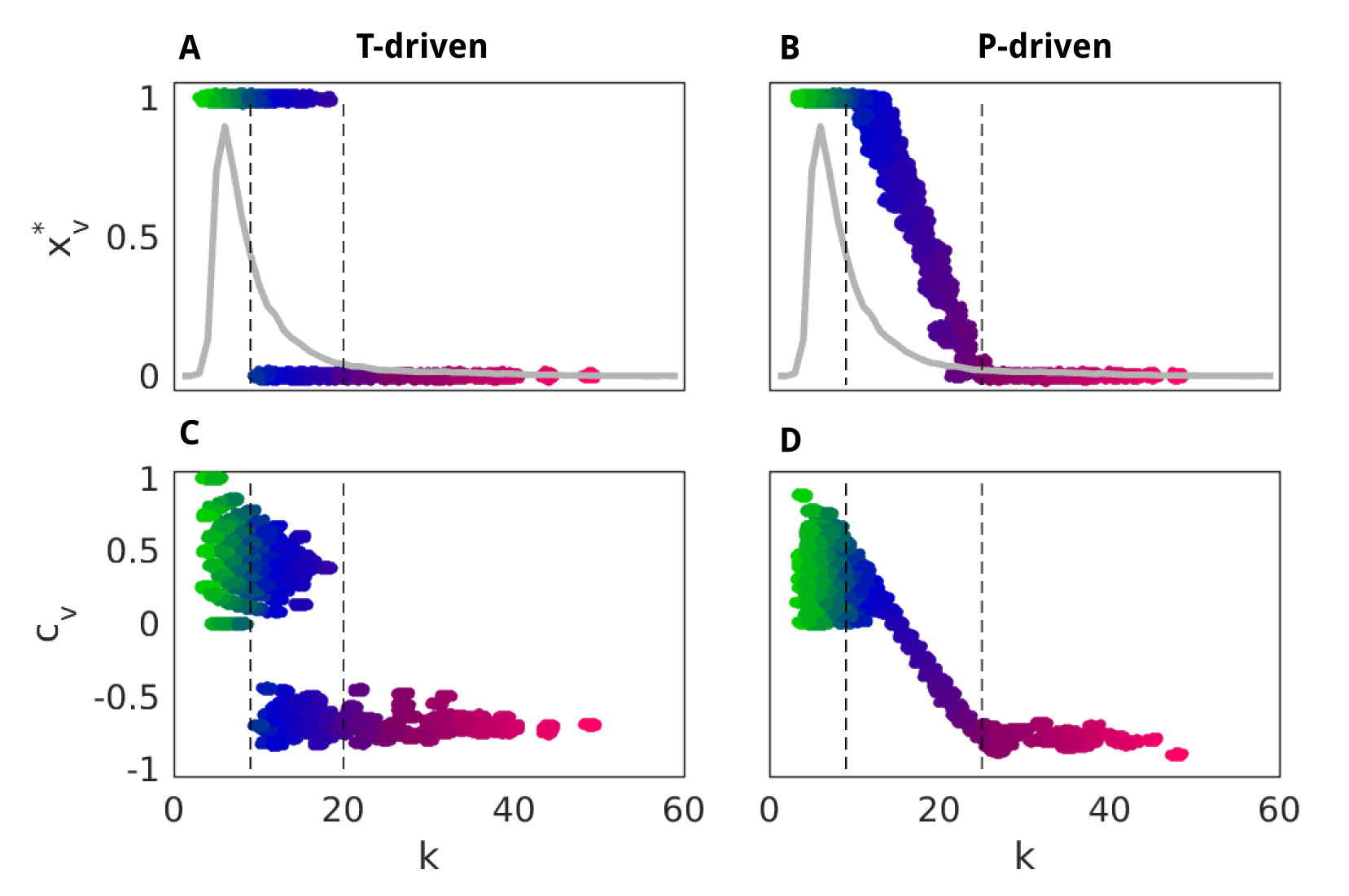
Figure 5: Selfishness and altruism within heterogeneous populations. Steady steady state configurations for T-driven (subplot A) and P-driven (subplot B) games. The results have been obtained by simulating the SR-EGN equation for $500$ realizations of a SF network, composed by $N=100$ individuals, with average degree $\bar{k}=10$. The self regulation parameter is set to $\beta=15$ for all players. The transition from green to blue to magenta indicates the social role of players in the graphs, thus allowing to distinguish between non central players (green dots), intermediate player (blue dots) and hubs (magenta dots). The vertical dashed lines highlight this distinction. The grey lines represent the degree distribution of the networks. Subplots C and D report the indicator $c_{v}$ introduced in equation (8), for the T-driven and P-driven games, respectively.

Additionally, the relationship between $\beta_{v}$ and $k_{v}$ is highlighted in Figure 5 where $\beta$ is set to $15$, and SF networks are used. For each player, a circle represents the reached steady state as a function of his in-degree (Figures 5A and 5B). In the same subplots, the degree distributions of networks is depicted in gray. Players with low degree (green dots), representing non-central individuals, converge towards a cooperative steady state. On the other hand, hub players (magenta dots), always prefer defection. Players with intermediate in-degree (blue dots) show different behaviors for the T-driven and P-driven games. Specifically, these players split into two subgroups showing different behaviors (some full cooperators and some full defectors, see Figure 5A). Figure 5B shows that these type of players reach a partial level of cooperation. The distinction of the three groups is highlighted by the dashed vertical black lines.

In order to quantify the difference between the level of cooperation of player $v$ and the average cooperation of his neighbors at steady state, the following quantitative indicator is introduced:

$$c_{v}=x_{v}^{*}-\frac{1}{k_{v}}\sum_{w=1}^{N}a_{v,w}x_{w}^{*}.$$ (8)

If $c_{v}>0$, then player $v$ is altruistic, since his level of cooperation is higher than the average of his neighbors, while $c_{v}<0$ indicates more selfish behaviors. The group of non central players is always more altruistic than hubs. The intermediate players are again splitted into altruist and selfish for T-driven game (Figure 5C), while for P-driven game (Figure 5D), this distinction vanishes, and a continuous distribution of altruist and selfish persons is observed.

Joining the results of Figures 3, 4 and 5, we conclude that some individuals are more sensitive and aware on their internal mechanisms, thus becoming cooperative for lower self-regulating factors, and exhibiting a more altruistic behavior. In particular, for the P-driven game, these receptive individuals catalyze the others to cooperate.

Appendix A The Evolutionary Game equation on Networks (EGN) and self games

Let $\mathcal{V}=\{1,2,\ldots,N\}$ be the set of players. Each player is placed in a vertex of a directed graph, defined by the adjacency matrix ${\bf A}=\{a_{v,w}\}\in\{0,1\}^{N\times N}$ with ${(v,w)\in\mathcal{V}^{2}}$. Specifically, $a_{v,w}=1$ when $v$ is connected with $w$, $0$ otherwise. It is also assumed that $a_{v,v}=0$. The degree of player $v$ is defined as the cardinality of his neighborhood, namely:

$$k_{v}=\sum_{w=1}^{N}a_{v,w}.$$

In the literature on evolutionary game theory, it is assumed that, at each time, one individual uses a pure strategy in a given set while playing games with connected individuals. For the specific topic of cooperation, these games are often modeled as Prisoner’s dilemma games: the set of pure strategies contains only two elements, cooperation ($C$) and defection ($D$), and the outcome is described by the following payoff matrix:

$${\bf B}=\begin{bmatrix}R&S\\ T&P\end{bmatrix},$$

where $R$ is the reward when both players cooperate, $T$ is the temptation to defect when the opponent cooperates, $S$ is the sucker’s payoff earned by a cooperative player when the opponent defects, and $P$ is the punishment for mutual defection. More specifically, for a Prisoner’s dilemma game, the reward is a better outcome than the punishment ($R>P$), the temptation payoff is higher than the reward ($T>R$), and the punishment is preferred to the sucker’s payoff ($P>S$). It is useful to define $\sigma_{C}=R-T<0$ and $\sigma_{D}=P-S>0$ [37], allowing us to distinguish two cases: when the effect of $\sigma_{C}$ is stronger than $\sigma_{D}$ ($|\sigma_{C}|>\sigma_{D}$) we will refer to a T-driven game, while the opposite situation ($|\sigma_{C}|<\sigma_{D}$) is hereafter called P-driven game.

In the present work, a more realistic scenario is investigated, where one player can choose his own level of cooperation, instead of just $C$ or $D$. The level of cooperation of a generic player $v$, is denoted by the real number $x_{v}\in[0,1]$; specifically, $x_{v}=1$ stands for a player exhibiting maximum cooperativeness, while $x_{v}=0$ represents a full defector. All other shades (i.e. $x_{v}\in(0,1)$) denote partial levels of cooperation. In this new framework, when any two connected players $v$ and $w$ take part in a game, the payoff for $v$ is defined by the continuous bilinear function $\phi:[0,1]\times[0,1]\to\mathbb{R}$:

$$\phi(x_{v},x_{w}) = [x_{v},1-x_{v}]{\bf B}\begin{bmatrix}x_{w}\\ 1-x_{w}\end{bmatrix}$$

$$= (R-T+P-S)x_{v}x_{w}-(P-S)x_{v}-(P-T)x_{w}+P.$$

Moreover, notice that $x_{v},x_{w}\in\{0,1\}$, we recover the payoffs $R$, $T$, $S$ and $P$.

The total payoff of player $v$ is the sum of all outcomes of two-player games with neighbors. Formally, the payoff function $\phi_{v}:[0,1]^{N}\to\mathbb{R}$ is defined as follows:

$$\phi_{v}({\bf x})=\sum_{w=1}^{N}a_{v,w}\phi(x_{v},x_{w}),$$

where ${\bf x}$ is the vector of all the $x_{v}$ variables. Moreover, given the vector ${\bf x}$, we define the following payoff of pure strategies $C$ ($x_{v}=1$) and $D$ ($x_{v}=0$):

$$\begin{cases}p_{v}^{C}({\bf x})=\displaystyle\sum_{w=1}^{N}a_{v,w}\phi(1,x_{w})=\displaystyle\sum_{w=1}^{N}a_{v,w}((R-S)x_{w}+S)\\ p_{v}^{D}({\bf x})=\displaystyle\sum_{w=1}^{N}a_{v,w}\phi(0,x_{w})=\displaystyle\sum_{w=1}^{N}a_{v,w}((T-P)x_{w}+P)\\ \end{cases}.$$

Following [35, 36], the EGN equation for two-strategy games reads as follows:

$$\dot{x}_{v}=x_{v}(1-x_{v})\Delta p_{v}({\bf x}),$$ (9)

where

$$\Delta p_{v}({\bf x})=p_{v}^{C}({\bf x})-p_{v}^{D}({\bf x}) = \displaystyle\sum_{w=1}^{N}a_{v,w}(R-T+P-S)x_{w}-(P-S))$$

$$= \displaystyle\sum_{w=1}^{N}a_{v,w}((\sigma_{C}+\sigma_{D})x_{w}-\sigma_{D}).$$

It is clear that the level of cooperation of player $v$ increases (decreases) when $\Delta p_{v}({\bf x})$ is positive (negative). In other words, the player $v$ will be more cooperative over time as long as the payoff he can earn using the pure strategy $C$ is better than the payoff he can earn using the pure strategy $D$.

This comparative evaluation of the benefits provided by the available strategies can be represented in an alternative way. Specifically, suppose that player $v$ is able to appraise whether a change of his strategy $x_{v}$ produces an improvement of his payoff $\phi_{v}$. This means that, if the derivative of $\phi_{v}$ with respect to $x_{v}$ is positive (negative), the player would like to increase (decrease) his level of cooperation. Interestingly, the following result holds:

$$\frac{\partial\phi_{v}({\bf x})}{\partial x_{v}} = \sum_{w=1}^{N}a_{v,w}\frac{\partial\phi(x_{v},x_{w})}{\partial x_{v}}$$

$$= \sum_{w=1}^{N}a_{v,w}\left((R-T+P-S)x_{w}-(P-S)\right),$$

$$= \sum_{w=1}^{N}a_{v,w}\left((\sigma_{C}+\sigma_{D})x_{w}-\sigma_{D}\right),$$

$$= \Delta p_{v}({\bf x}).$$

Thus, the EGN equation (9) can be rewritten as follows:

$$\dot{x}_{v}=x_{v}(1-x_{v})\frac{\partial\phi_{v}({\bf x})}{\partial x_{v}}.$$ (10)

It is worthwhile to notice that, while the replicator equation is used to describe the dynamics of population where strategies correspond to the phenotypes of the individuals, its extension on graphs, the EGN equation, is suitable for analyzing the dynamics of individuals arranged on a network, which are able to choose their strategies in the continuous set $[0,1]$.

The EGN equation (10), as well as most of the models presented in the literature, assumes that the strategy dynamics of a generic player $v$ is driven only by external factors. Indeed, $\frac{\partial\phi_{v}}{\partial x_{v}}$ depends only on the state of neighboring players, not on the current state $x_{v}$ of player $v$ himself. Inspired by mechanisms describing self-regulation in animal societies reported in [39], we overcome this issue by introducing the Self-Regulated EGN equation (SR-EGN); this new model is obtained by adding a self-regulating term $f_{v}$ to the EGN equation, balancing the external feedback $\frac{\partial\phi_{v}}{\partial x_{v}}$, thus reading as follows:

$$\dot{x}_{v}=x_{v}(1-x_{v})\left(\frac{\partial\phi_{v}({\bf x})}{\partial x_{v}}-\beta_{v}f_{v}(x_{v})\right),$$ (11)

where the parameter $\beta_{v}$ is used to tune the effectiveness of the introduced self-regulation mechanism. Specifically, we assume that this self-regulation term embodies a game that a given individual plays against himself. To describe this self game, consider two generic players which strategies are $y$ and $z$, both belonging to the set $[0,1]$. As already mentioned, the first player can assess whether a change of his strategy $y$ can lead to an improvement of the payoff $\phi(y,z)$. In particular, the assessment is based on the sign of the partial derivative

$$\frac{\partial\phi(y,z)}{\partial y}=(\sigma_{C}+\sigma_{D})z-\sigma_{D}.$$

In the particular case of individuals representing both the first and second player at the same time, the derivative reads as follows:

$$\left.\frac{\partial\phi(y,z)}{\partial y}\right|_{y=z=x_{v}}=(\sigma_{C}+\sigma_{D})x_{v}-\sigma_{D}.$$

Therefore, the self-regulating term is defined as:

$$f_{v}(x_{v})=\left.\frac{\partial\phi(y,z)}{\partial y}\right|_{y=z=x_{v}}=(\sigma_{C}+\sigma_{D})x_{v}-\sigma_{D}.$$

It is worthwhile to notice that the time derivative of $x_{v}$ in (11) depends on $x_{v}$ in the term accounting for the self game. Thus, the self game introduces a feedback mechanism regulated by the parameter $\beta_{v}\in\mathbb{R}$. In particular, in equation (11), $\beta_{v}>0$ represents a negative feedback, $\beta_{v}<0$ stands for a positive feedback, while $\beta_{v}=0$ refers to situations where the player $v$ does not play a self game.

A.1 Steady states and linearization

A steady state $\bf{x^{*}}$ is a solution of equation (11) satisfying $\dot{x}_{v}=0~{}\forall v\in\mathcal{V}$. In order to be feasible, the components of a steady state must belong to the set $[0,1]$. Formally, the set of feasible steady states is:

$$\Theta=\{{\bf x}^{*}\in\mathbb{R}^{N}:\dot{x}_{v}^{*}=0\wedge x_{v}^{*}\in[0,1]~{}\forall v\in\mathcal{V}\}.$$

It is clear that all points such that for all $v$, $x_{v}^{*}=0$ or $x_{v}^{*}=1$ are in the set $\Theta$. They are the $2^{N}$ pure steady states. We remark that set $\Theta$ may contain also other steady states, exhibiting fuzzy levels of cooperation. Particularly relevant are the pure steady states

$${\bf x}^{*}_{ALLC}=[1,1,\ldots,1]^{\top},$$

and

$${\bf x}^{*}_{ALLD}=[0,0,\ldots,0]^{\top}.$$

Indeed, they represent a population composed by full cooperators and full defectors, respectively, and thus they describe the spread of cooperation and its extinction in a given population.

The dynamical properties of these two pure steady states is fundamental for the emergence of cooperation. In particular, their stability can be analyzed by linearizing system (11) near them.

The Jacobian matrix of system (10), ${\bf J}({\bf x})=\{j_{v,w}({\bf x})\}$, is defined as follows:

$$j_{v,w}({\bf x})=\frac{\partial\dot{x}_{v}}{\partial x_{w}}=\begin{cases}x_{v}(1-x_{v})(\sigma_{C}+\sigma_{D}),&\text{if}~{}a_{v,w}=1\\ ~{}\\ (1-2x_{v})\displaystyle\left(\frac{\partial\phi_{v}({\bf x})}{\partial x_{v}}-\beta_{v}f_{v}(x_{v})\right)-\beta_{v}x_{v}(1-x_{v})(\sigma_{C}+\sigma_{D}),&\text{if}~{}w=v\\ ~{}\\ 0,&\text{otherwise}\end{cases}.$$

It is easy to show that the Jacobian matrix reduces to a diagonal one for both ${\bf x}^{*}_{ALLC}$ and ${\bf x}^{*}_{ALLD}$. Moreover, observe that:

$$\frac{\partial\phi_{v}({\bf x}^{*}_{ALLC})}{\partial x_{v}} = \sum_{w=1}^{N}a_{v,w}((\sigma_{C}+\sigma_{D})\cdot 1-\sigma_{D})=\sum_{w=1}^{N}a_{v,w}\sigma_{C}=k_{v}\sigma_{C},$$

$$\frac{\partial\phi_{v}({\bf x}^{*}_{ALLD})}{\partial x_{v}} = \sum_{w=1}^{N}a_{v,w}((\sigma_{C}+\sigma_{D})\cdot 0-\sigma_{D})=-\sum_{w=1}^{N}a_{v,w}\sigma_{D}=-k_{v}\sigma_{D},$$

$$f_{v}(1) = (\sigma_{C}+\sigma_{D}\cdot 1-\sigma_{D})=\sigma_{C},$$

$$f_{v}(0) = (\sigma_{C}+\sigma_{D}\cdot 0-\sigma_{D})=-\sigma_{D}.$$

Therefore, we have that:

$$j_{v,v}({\bf x}^{*}_{ALLC})=(1-2\cdot 1)\displaystyle\left(\frac{\partial\phi_{v}({\bf x}^{*}_{ALLC})}{\partial x_{v}}-\beta_{v}f_{v}(1)\right)=-\sigma_{C}(k_{v}-\beta_{v})$$

for ${\bf x}^{*}_{ALLC}$, and

$$j_{v,v}({\bf x}^{*}_{ALLD})=(1-2\cdot 0)\displaystyle\left(\frac{\partial\phi_{v}({\bf x}^{*}_{ALLD})}{\partial x_{v}}-\beta_{v}f_{v}(0)\right)=-\sigma_{D}(k_{v}-\beta_{v})$$

for ${\bf x}^{*}_{ALLD}$.

Appendix B Emergence of cooperation in the EGN equation with self-regulations

The emergence of cooperation is reached when all the members of a social network turn their strategies to cooperation. Therefore, the asymptotic stability of ${\bf x}^{*}_{ALLC}$, as well as the instability of ${\bf x}^{*}_{ALLD}$, has a fundamental role in this context. In order to study the stability of steady states ${\bf x}^{*}_{ALLC}$ and ${\bf x}^{*}_{ALLD}$, we start by analyzing their linear stability. Moreover, an appropriate Lyapunov function is proposed, which prove that ${\bf x}^{*}_{ALLC}$ is also globally asymptotically stable, thus guarantying the emergence of cooperation.

B.1 Asymptotic stability of ${\bf x}^{*}_{ALLC}$

Recall that the spectrum of ${\bf J}({\bf x}^{*})$ characterizes the linear stability of any steady state ${\bf x}^{*}$ [40]. Therefore, the role of the eigenvalues of the Jacobian matrix ${\bf J}({\bf x}^{*})$ is fundamental to tackle the problem of the emergence of cooperation.

The following results hold.

Theorem 1.

If $\beta_{v}>k_{v}~{}\forall v\in\mathcal{V}$, then ${\bf x}^{*}_{ALLC}$ is asymptotically stable.

Proof.

As shown before, the Jacobian matrix evaluated for ${\bf x}^{*}_{ALLC}$ is diagonal. Then, the elements on the diagonal of the Jacobian matrix correspond to its eigenvalues and they are defined as follows:

$$j_{v,v}({\bf x}^{*}_{ALLC})=\lambda_{v}=-\sigma_{C}(k_{v}-\beta_{v}).$$

Using the fact that $\beta_{v}>k_{v}~{}\forall v\in\mathcal{V}$, and $\sigma_{C}<0$, all the eigenvalues are negative. Thus, ${\bf x}^{*}_{ALLC}$ is asymptotically stable. ∎

Theorem 2.

If $\exists v\in\mathcal{V}:\beta_{v}>k_{v}$, then ${\bf x}^{*}_{ALLD}$ is unstable.

Proof.

The eigenvalues of the Jacobian matrix relative to the steady state ${\bf x}^{*}_{ALLD}$ are

$$j_{v,v}({\bf x}^{*}_{ALLD})=\lambda_{v}=-\sigma_{D}(k_{v}-\beta_{v}).$$

If the hypothesis of the theorem are fulfilled, since $\sigma_{D}>0$, then there is at least one positive eigenvalue, implying that ${\bf x}^{*}_{ALLD}$ is an unstable steady state. ∎

These results are summarized as follows: defection dominates over cooperation. Then, if the system does not present any internal feedback mechanism (i.e. $\beta_{v}=0~{}\forall v\in\mathcal{V}$), the whole social network will converge to ${\bf x^{*}}_{ALLD}$ (cooperation vanishes). Anyway, using $\beta_{v}>k_{v}$ for all the members of the population, ${\bf x^{*}}_{ALLD}$ is destabilized and ${\bf x^{*}}_{ALLC}$ becomes attractive.

B.2 Global asymptotic stability of ${\bf x}^{*}_{ALLC}$

Theorems 1 and 2 prove that under suitable condition, ${\bf x}^{*}_{ALLC}$ is asymptotically stable and ${\bf x}^{*}_{ALLD}$ is unstable. Anyway, this is not sufficient to prove emergence of cooperation. Indeed, there can be some other steady states in $\Theta$ which may be also attractive. Nevertheless, a Lyapunov function for the steady state ${\bf x}^{*}_{ALLC}$ on the set ${\bf x}\in(0,1]^{N}$ can be found [42].

Adapting the approach presented in [37, 41] to the SR-EGN equation, we consider the following function:

$$V({\bf x})=-\sum_{v=1}^{N}\log(x_{v}),$$

for ${\bf x}\in(0,1]^{N}$. Notice that $V({\bf x}^{*}_{ALLC})=0$, and $V({\bf x})>0~{}\forall{\bf x}\neq{\bf x}^{*}_{ALLC}$.

Moreover, the time derivative of $V({\bf x})$ is defined as follows:

$$\dot{V}({\bf x})=\frac{\partial V({\bf x})}{\partial t} = \sum_{v=1}^{N}\frac{\partial V({\bf x})}{\partial x_{v}}\dot{x}_{v}=$$ (12)

$$= -\sum_{v=1}^{N}\frac{1}{x_{v}}x_{v}(1-x_{v})\left(\frac{\partial\phi_{v}({\bf x})}{\partial x_{v}}-\beta_{v}f_{v}(x_{v})\right)=$$

$$= \sum_{v=1}^{N}(x_{v}-1)\left(\frac{\partial\phi_{v}({\bf x})}{\partial x_{v}}-\beta_{v}f_{v}(x_{v})\right).$$

Finally, it is clear that $\dot{V}({\bf x}_{ALLC}^{*})=0$.

Starting from these premises, if $\dot{V}({\bf x})<0$ for all ${\bf x}\in(0,1]^{N}\setminus\{{\bf x}^{*}_{ALLC}\}$, then $V({\bf x})$ is a Lyapunov function.

Let’s introduce the following quantities:

$$\psi=\inf_{y\in(0,1]}(\sigma_{C}+\sigma_{D})y-\sigma_{D},$$ (13)

$$\xi=\sup_{y\in(0,1]}(\sigma_{C}+\sigma_{D})y-\sigma_{D},$$ (14)

and

$$\rho=\frac{\psi}{\xi}.$$

Notice that, since $\sigma_{C}<0$ and $\sigma_{D}>0$, then both $\psi$ and $\xi$ are negative. Indeed,

• for a T-driven game, since $|\sigma_{C}|>\sigma_{D}$, then $\psi=\sigma_{C}$ and $\xi=-\sigma_{D}$;

• for a P-driven game, since $|\sigma_{C}|<\sigma_{D}$, then $\psi=-\sigma_{D}$ and $\xi=\sigma_{C}$.

Then, we conclude that $\rho$ is a positive number if both cases, and, in particular, it is:

$$\rho=\frac{\psi}{\xi}=\begin{cases}\displaystyle\left|\frac{\sigma_{C}}{\sigma_{D}}\right|&\text{for {\it T-driven} games}\\ \\ \displaystyle\left|\frac{\sigma_{D}}{\sigma_{C}}\right|&\text{for {\it P-driven} games}.\end{cases}$$

The following result holds.

Theorem 3.

If $\beta_{v}>\rho k_{v}~{}\forall v\in\mathcal{V}$, then $V({\bf x})$ is a Lyapunov function.

Proof.

It is straightforward to see that:

$$\frac{\partial\phi_{v}({\bf x})}{\partial x_{v}}=\sum_{w=1}^{N}a_{v,w}((\sigma_{C}+\sigma_{D})x_{w}-\sigma_{D})\geq\sum_{w=1}^{N}a_{v,w}\psi=k_{v}\psi.$$ (15)

Similarly, since $\beta_{v}>0$, we get that:

$$\beta_{v}f_{v}(x_{v})=\beta_{v}((\sigma_{C}+\sigma_{D})x_{v}-\sigma_{D})\leq\beta_{v}\xi.$$ (16)

Joining (15) and (16) together, we get that:

$$\frac{\partial\phi_{v}({\bf x})}{\partial x_{v}}-\beta_{v}f_{v}(x_{v})\geq k_{v}\psi-\beta_{v}\xi.$$

Moreover, notice that:

$$\beta_{v}>\rho k_{v}\Rightarrow\beta_{v}>\frac{\psi}{\xi}k_{v}\Rightarrow k_{v}\psi-\beta_{v}\xi>0,$$

and hence

$$\frac{\partial\phi_{v}({\bf x})}{\partial x_{v}}-\beta_{v}f_{v}(x_{v})>0~{}\forall v\in\mathcal{V}.$$ (17)

According to equations (12) and (17), since $x_{v}-1<0$ for all ${\bf x}\in(0,1]^{N}\setminus\{{\bf x}^{*}_{ALLC}\}$, we guarantee that $\dot{V}({\bf x})<0$ for all ${\bf x}\in(0,1]^{N}\setminus\{{\bf x}^{*}_{ALLC}\}$. Hence, $V({\bf x})$ is a Lyapunov function. ∎

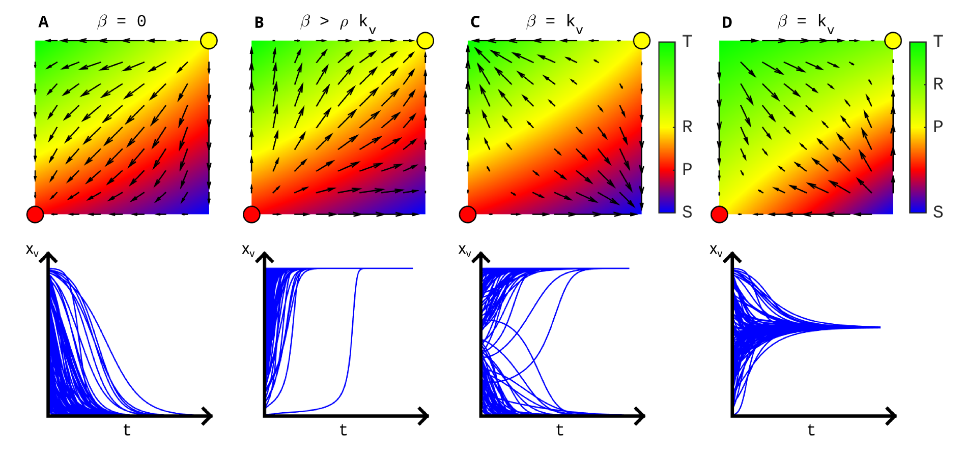
Figure 6: Payoff, flow and dynamics. Value of the two-player game payoff $\phi(x_{v},x_{w})$, and corresponding flow of the SR-EGN equation in the phase space $(x_{v},x_{w})$ for different values of $\beta_{v}$. Subplots A, B and C: T-driven game ($\sigma_{C}=-2$ and $\sigma_{D}=1$); subplot D: P-driven game ($\sigma_{C}=-1$ and $\sigma_{D}=2$). Red and yellow circles represent the steady states ${\bf x}_{ALLD}^{*}$ and ${\bf x}_{ALLC}^{*}$, respectively. For each case, the corresponding dynamics for a population of $N=100$ players arranged on a scale-free network with average degree $\bar{k}=10$ is depicted below, where initial conditions are randomly chosen in the set $(0,1)$. Results for $\beta_{v}=0$ and $\beta_{v}>\rho k_{v}$ in the T-driven game are similar to the P-driven game, thus not reported here.

Figure 6 compares the above theoretical results to the standard case ($\beta_{v}=0$), by showing the flow in phase space of EGN and SR-EGN equations, and the corresponding time course of the cooperation level for a population of $N=100$ players organized on a scale-free network. Figures 6A and 6B show that all players are attracted by full defection (EGN) and full cooperation (SR-EGN), respectively. The same scheme has been used to investigate the marginal case $\beta_{v}=k_{v}$ in the T-driven (Figure 6C) and P-driven (Figure 6D) games. In the first case, some players are attracted by full cooperation and some others by full defection, while in the second we observe the presence of an attracting line of partially cooperative steady states, where all players share the same level of cooperation. In this case, the different level reached depends on the initial conditions.

References

- [1] P. Hammerstein, Ed., Genetic and Cultural Evolution of Cooperation. (MIT Press, Cambridge, MA, 2003).
- [2] M.A. Nowak, K. Sigmund, Evolutionary dynamics of biological games. Science 303, 793-799 (2004).
- [3] M. Doebeli, C. Hauert, T. Killingback, The evolutionary origin of cooperators and defectors. Science 306, 859-862 (2004).
- [4] H. Gintis, Ed., Moral sentiments and material interests: The foundations of cooperation in economic life (MIT Press, Cambridge, MA, 2005), vol. 6.
- [5] E. Pennisi, On the origin of cooperation. Science 325, 1196–1199 (2009).
- [6] D.G.Rand, M.A. Nowak, Human cooperation, Trends Cogn. Sci. 17, 413-425 (2013).
- [7] Cao, Y., Yu, W., Ren, W., Chen, G. An overview of recent progress in the study of distributed multi-agent coordination. IEEE T. Ind. Inform. 9, 427-438 (2013).
- [8] D.F.P. Toupo, S.H. Strogatz, J.D. Cohen, D.G. Rand, Evolutionary game dynamics of controlled and automatic decision-making. Chaos 25, 073120 (2015).
- [9] Gray, R., Franci, A., Srivastava, V., Leonard, N. E. Multi-agent decision-making dynamics inspired by honeybees. IEEE T. Cont. Netw. Syst. (2018).
- [10] E. Fehr, U. Fischbacher, Social norms and human cooperation. Trends Cogn. Sci. 8, 185-190 (2004).
- [11] C. Hauert, A. Traulsen, H. Brandt, M.A. Nowak, K. Sigmund, K. Via freedom to coercion: the emergence of costly punishment. Science 316, 1905-1907 (2007).
- [12] E. Fehr, S. Gachter, Altruistic punishment in humans. Nature 415, 137–140 (2002).
- [13] B. Hannelore, C. Hauert, K. Sigmund, Punishment and reputation in spatial public goods games. P. Roy. Soc. Lond. B Bio. 270, 1099-1104 (2003).
- [14] R. Boyd, H. Gintis, S. Bowles, Coordinated punishment of defectors sustains cooperation and can proliferate when rare. Science 328, 617-620 (2010).
- [15] D. Helbing, A. Johansson, Cooperation, Norms, and Revolutions: A Unified Game-Theoretical Approach. PLoS ONE 5, e12530 (2010).
- [16] D.G. Rand, M.A. Nowak, The evolution of anti-social punishment in optional public goods games. Nat. Comm. 2, 434 (2011).
- [17] X. Li, M. Jusup, Z. Wang, H. Li, L. Shi, B. Podobnik, H. E. Stanley, S. Havlin, S. Boccaletti, Punishment diminishes the benefits of network reciprocity in social dilemma experiments. P. Natl. Acad. Sci. USA 201707505 (2017).
- [18] M.A. Nowak, Five rules for the evolution of cooperation. Science 314, 1560-1563 (2006).
- [19] Z. Wang, M. Jusup, R. Wang, L. Shi, Y. Iwasa, Y. Moreno, J. Kurths, Onymity promotes cooperation in social dilemma experiments. Sci. Adv. 3, e1601444 (2017).
- [20] C. Hauert, F. Michor, M.A. Nowak, M. Doebeli, Synergy and discounting of cooperation in social dilemmas. J. Theor. Biol. 239, 195–202 (2006).
- [21] F.C. Santos, M.D. Santos, J.M. Pacheco, Social diversity promotes the emergence of cooperation in public goods games. Nature 454, 213-26 (2008).
- [22] D.G. Rand, A. Dreber, T. Ellingsen, D. Fudenberg, M.A. Nowak, Positive interactions promote public cooperation. Science 325, 1272-1275 (2009).
- [23] J. Hofbauer, K. Sigmund. Evolutionary games and population dynamics (Cambridge University Press, 1998).
- [24] M.A. Nowak, A. Sasaki, C. Taylor, D. Fudenberg, Emergence of cooperation and evolutionary stability in finite populations. Nature 428, 646–650 (2004).
- [25] H. Ohtsuki, C. Hauert, E. Lieberman, M.A. Nowak, A simple rule for the evolution of cooperation on graphs and social networks. Nature 441, 502-505 (2006).
- [26] Santos, F.C. & Pacheco, J.M. Scale-free networks provide a unifying framework for the emergence of cooperation. Phys. Rev. Lett. 95, 098104 (2005).
- [27] E. Lieberman, C. Hauert, M.A. Nowak, Evolutionary dynamics on graphs. Nature 433, 312-316 (2005).
- [28] F.C. Santos, J.M. Pacheco, T. Lenaerts, Evolutionary dynamics of social dilemmas in structured heterogeneous populations. P. Natl. Acad. Sci. USA 103, 3490–3494 (2006).
- [29] Ohtsuki, H., Nowak, M. A. The replicator equation on graphs. J. Theor. Biol. 243, 86-96 (2006).
- [30] L. Dall’Asta, M. Marsili, and P. Pin, Collaboration in social networks. P. Natl. Acad. Sci. USA 109, 4395–4400 (2015).
- [31] C. Adami, J. Schossau, A. Hintze, Evolutionary game theory using agent-based methods. Phys. Life Rev. 19, 1-26 (2016).
- [32] B. Allen et al. Evolutionary dynamics on any population structure, Nature 544, 227-230 (2017).
- [33] J. Gómez-Gardeñes, I. Reinares, A. Arenas, L.M. Floría, Evolution of Cooperation in Multiplex Networks. Sci. Rep. 2 (2012).
- [34] G. Vogel, “The evolution of the golden rule: humans and other primates have a keen sense of fairness and a tendency to cooperate, even when it does them no discernible good”. Science 303, 1128-1131 (2004).
- [35] D. Madeo, C. Mocenni, Game Interactions and dynamics on networked populations. IEEE T. Automat. Contr. 60, 1801-1810 (2015).
- [36] G. Iacobelli, D. Madeo, C. Mocenni, Lumping evolutionary game dynamics on networks. J. Theor. Biol. 407, 328-338 (2016).
- [37] Weibull, J. Evolutionary Game Theory. (MIT Press, Cambridge, MA, 1995)
- [38] Z. Wang, S. Kokubo, M. Jusup, J. Tanimoto, Universal scaling for the dilemma strength in evolutionary games. Phys. Life Rev. 14, 1-30 (2015).
- [39] P. Schuster, K. Sigmund, J. Hofbauer, R. Gottlieb, P. Merz, Selfregulation of behaviour in animal societies. Biol. Cybern. 40, 17-25 (1981).
- [40] Strogatz, S.H. Nonlinear Dynamics and Chaos: With Applications to Physics, Biology, Chemistry and Engineering (Westview Press, Boulder, CO, Usa, 2001).
- [41] Hofbauer, J. & Sigmund, K. Evolutionary Games and Population Dynamics (Cambridge, UK: Cambridge Univ. Press, 1998).
- [42] Khalil, H. K. Nonliner systems (NJ: Prentice-Hall, 2002).
Acknowledgments
CM was partially supported by grant 313773/2013-0 of the Science without Borders Program of CNPq/Brazil.