Thermoelectric characterization of the Kondo resonance in nanowire quantum dots

Abstract

We experimentally verify hitherto untested theoretical predictions about the thermoelectric properties of Kondo correlated quantum dots (QDs). The specific conditions required for this study are obtained by using QDs epitaxially grown in nanowires, combined with a recently developed method for controlling and measuring temperature differences at the nanoscale. This makes it possible to obtain data of very high quality both below and above the Kondo temperature, and allows a quantitative comparison with theoretical predictions. Specifically, we verify that Kondo correlations can induce a polarity change of the thermoelectric current, which can be reversed either by increasing the temperature or by applying a magnetic field.

Measurements of electric and thermoelectric transport properties can be used to reveal and characterize novel strongly correlated phases, which often appear in meso- and nano-scale systems. The Kondo effect Kondo (1964) is a prominent example where interactions between conduction electrons and magnetic impurities result in a many-body singlet state involving the impurity spin and a large number of conduction electrons. In metals it leads to increased resistivity at low temperatures where the magnetic impurity scattering dominates. More recently, quantum dots (QDs) tunnel-coupled to two leads have provided a platform for more detailed experimental studies of the Kondo effect Goldhaber-Gordon et al. (1998); Cronenwett et al. (1998); Nygård et al. (2000). In QDs, the Kondo scattering lifts the Coulomb blockade Ng and Lee (1988); Glazman and Raikh (1988); Hewson (1993) and gives rise to a peak in the differential conductance $g=dI/dV$ around $V=0$ ($I$ is the current and $V$ is the bias voltage).

Several theoretical works (see, e.g., Refs Boese and Fazio (2001); Costi and Zlatic (2010); Roura-Bas et al. (2012); Azema et al. (2012); Weymann and Barnaś (2013); Ye et al. (2014); Dorda et al. (2016); Sierra et al. (2017); Karki and Kiselev (2017)) have proposed that additional insights into Kondo physics can be gained from thermoelectric measurements. Here, a temperature difference $\Delta T=T_{c}-T_{h}$ is applied between a hot ($h$) and a cold ($c$) lead and one measures either the resulting thermocurrent $I_{th}$ (measured under closed-circuit conditions), or the thermovoltage $V_{th}$ (measured under open-circuit conditions). In QDs without Kondo correlations, $I_{th}$ and $V_{th}$ have characteristic shapes as functions of the gate voltage, $V_{G}$, exhibiting a sign reversal (zero crossing) at each charge degeneracy point as well as in the center of each Coulomb valley Beenakker and Staring (1992); Staring et al. (1993); Dzurak et al. (1993). It has been theoretically predicted Costi and Zlatic (2010) that Kondo correlations would significantly change this behavior by removing some zero crossings and consequently reversing the polarity of $I_{th}$ and $V_{th}$ over a finite $V_{G}$ range. Whether a QD shows the typical Kondo or non-Kondo behavior depends sensitively on several system parameters. Therefore, by observing the qualitative change in thermoelectric response as Kondo correlations are suppressed, e.g., by increased average temperature $T=(T_{h}+T_{c})/2$ or magnetic field $B$, one can not only gain insights into Kondo physics, but also probe the internal QD energy scales.

Despite such clear theoretical predictions, experimental studies of the thermoelectric properties of Kondo correlated QDs remain rather limited Scheibner et al. (2005); Svensson et al. (2013). Experimentally uncontrolled internal QD degrees of freedom often complicate even a qualitative comparison with theory. Therefore, the predicted reversal of $I_{th}$ and $V_{th}$ has been difficult to observe (although some unpublished data exist Thierschmann (2014)) and the response to a $B$ field has, to the best of our knowledge, not been investigated.

In this Letter, we take important steps towards filling this gap between experiments and theory by presenting thermoelectric measurements on several Kondo correlated QDs. We measure $I_{th}$ and $g(V\approx 0)=g_{0}$ over consecutive Kondo and non-Kondo Coulomb valleys. We observe the sign reversal of $I_{th}$ theoretically predicted for the Kondo regime, and measure the transition between Kondo and non-Kondo behavior as $T$ is increased, finding quantitative agreement with theory Costi and Zlatic (2010). Furthermore, we apply an external $B$ field which also destroys Kondo correlations and find that a surprisingly large $B$ is needed to recover the typical non-Kondo behavior.

Our observations necessitate overcoming significant experimental challenges to access the parameter regimes which most clearly reveal the Kondo correlations and allow detailed comparison with theory predictions. The requirements include: (i) strong quantum confinement such that transport is dominated by a single orbital ($\delta\epsilon\gg k_{B}T,\Gamma$, where $\delta\epsilon$ is the orbital spacing and $\Gamma$ is the tunnel coupling); (ii) large charging energy $U$ and tunnel coupling, and low temperature, such that the Kondo regime is reached ($U\gg\Gamma\gg k_{B}T$ and $T<T_{K}$, where $T_{K}$ is the Kondo temperature); (iii) application and characterization of $\Delta T$ across a very small QD; (iv) the ability to controllably tune the system in and out of the Kondo regime, e.g., by gating or by varying $T$ or $B$.

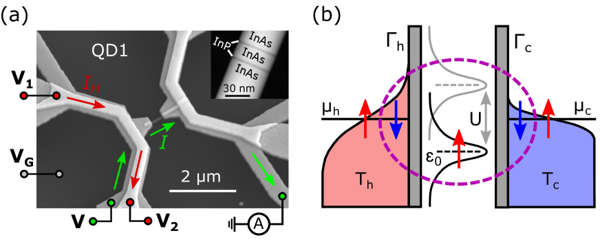
Figure 1: (a) Scanning electron microscope (SEM) image of device QD3. An InAs/InP nanowire containing a QD is contacted to metallic leads for electrical biasing with voltage $V$ (see SM SM for details on circuitry). Additional heater leads (lighter gray) enable application of a thermal bias $\Delta T$ to the QD by running a current $I_{H}$ resulting from a heater bias $V_{H}=V_{1}-V_{2}$. Only one heater is used in the experiment. Inset: Close-up scanning transmission electron microscope with high angle annular dark field (STEM-HAADF) image of an InAs/InP nanowire from the same growth. (b) Sketch of an unbiased spin-1/2 QD tunnel-coupled to two leads ($h$ and $c$).

To achieve the above requirements we use QDs epitaxially defined in axially heterostructured InAs/InP nanowires grown by chemical beam epitaxy Björk et al. (2004) [see inset in Fig. 1(a)]. Each InAs nanowire from the same growth is about 60 nm in diameter and contains two thin InP segments that confine an approximately 20 nm long InAs QD, similar to those used in our previous studies Svilans et al. (2016); Josefsson et al. (2017). The small QD size and the small effective mass of InAs give sufficiently large $U$ and $\delta\epsilon$, and the large g-factor allows tuning the Zeeman energy over a wide range. We use the fabrication process developed in Ref. Gluschke et al. (2014) to fabricate thermoelectric devices. Figure 1(a) shows a scanning electron microscope (SEM) image of the device QD1. In short, the devices are fabricated on an n-doped Si wafer coated with $\mbox{SiO}_{2}$. Two Ni/Au leads are used to contact the outer InAs segments on each side of the QD. The nanowires along with the contacting leads are coated with $\mbox{HfO}_{2}$ in order to electrically isolate the heater leads from the electrical biasing circuit Gluschke et al. (2014); Svilans et al. (2016). A back contact to the Si wafer is at a voltage $V_{G}$ and allows for electrostatic gating of the epitaxially defined QDs. We let $T_{h}$ and $T_{c}$ denote the temperatures of the nanowire leads contacting the QD, which might differ from those in the metallic leads further away. Application of a heating current $I_{H}$ increases both $T_{h}$ and (to a lesser degree) $T_{c}$, which in our devices gives control over $\Delta T$ and $T$ while maintaining a roughly constant $\Delta T/T\approx 0.30-0.35$. $T_{h}$ and $T_{c}$ are estimated based on QD thermometry (see Supplemental Material (SM) SM and Ref. Josefsson et al. (2017) for details). During this study we characterized three QDs (QD1, QD2 and QD3) showing similar behavior. Only the data from QD1 is presented with figures in the main text. Results on all devices are summarized in Table 1 (see SM SM for the corresponding data on other devices). The characterization was done in a dilution refrigerator with electron base temperature $T_{0}<100\mbox{ mK}$.

Figure 1(b) shows a sketch of a single-level QD with orbital energy $\varepsilon_{0}$ and onsite Coulomb repulsion $U$, coupled to leads by tunnel couplings $\Gamma_{h}$ and $\Gamma_{c}$ (Anderson model). The Kondo effect occurs when the level is occupied by a single electron. It originates from anti-ferromagnetic exchange interaction due to virtual exchange of electrons between the leads and the QD. Kondo correlations give rise to the formation of a singlet-like state (with binding energy $\sim k_{B}T_{K}$), involving the QD spin and a large number of electron spins in the leads. Below this energy the system behaves as a Fermi liquid and Coulomb blockade is lifted.

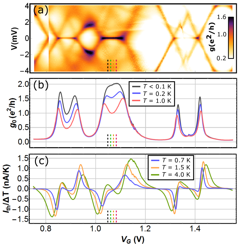
Figure 2: (a) $g$ as a function of $V$ and $V_{G}$, measured at $T=T_{0}<100$ mK. (b) The corresponding $g_{0}$ as a function of $V_{G}$ measured at three different $T$. (c) $I_{th}$ normalized by $\Delta T$ as a function of $V_{G}$ measured at three different $T$. The horizontal $V_{G}$ axis is the same in (a)–(c). Vertical dashed lines refer to $V_{G}$ values in Fig. 3.

We use Fig. 2 to identify the effects of Kondo correlations in the experimental data. The measured charge stability diagram at $T_{0}<100$ mK in Fig. 2(a) shows an increased $g_{0}$ inside Coulomb diamonds corresponding to odd electron numbers on the QD. In the absence of Kondo correlations one expects $g_{0}<e^{2}/h$, but Fig. 2(b) shows that (at $T=T_{0}$) $g_{0}$ approaches the limit $2e^{2}/h$, as expected in the Kondo regime. Increasing $T$ reduces $g_{0}$ in the odd occupancy Coulomb valleys but has little effect on valleys with even occupancy.

Figure 2(c) shows $I_{th}/\Delta T$ measured over the same gate range. We note that around $V_{G}=1.06$ V, where the strongest Kondo correlations are seen in (a) and (b), there is a qualitative change in $I_{th}(V_{G})$ with increasing $T$ with two sign reversals being absent at low $T$. Therefore, we focus our analysis on this particular $V_{G}$ range and come back to a detailed discussion of the thermoelectric behavior later.

Figure 3 presents the analysis for determining $T_{K}$ and $\Gamma$. We use the $T$ dependence of $g_{0}$ at the chosen $V_{G}$ range to determine $T_{K}$ using the phenomenological expression Goldhaber-Gordon et al. (1998); Kretinin et al. (2011)

$$g_{0}(T)=g_{0}(T=0)\left[1+\left(2^{1/s}-1\right)\left(\frac{T}{T_{K}}\right)^{2}\right]^{-s},$$ (1)

where $s=0.22$ for a spin-$1/2$ QD and $g_{0}(T=0)$ and $T_{K}$ are used as free fit parameters. Examples of the fits can be seen in the left panel of Fig. 3(a) while the corresponding $T_{K}$ fit values are plotted in Fig. 3(b). We also cross check the $T_{K}$ values by fitting the $V$ dependence of $g$ instead Pletyukhov and Schoeller (2012); SM . Examples of those fits are shown in the right panel of Fig. 3(a) while the corresponding fit values are plotted in Fig. 3(b). Overall, the two methods agree well, although the $V$ dependence of $g$ yields somewhat lower $T_{K}$ values.

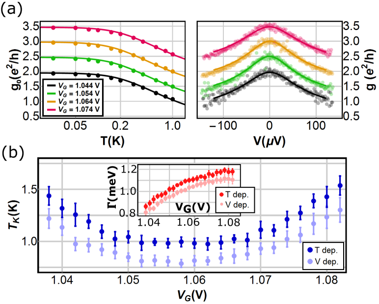
Figure 3: (a) Dots are the measured values of $g_{0}(T)$ in the left panel and of $g(V)$ at $T_{0}$ in the right panel, both for four different values of $V_{G}$, also indicated by vertical dashed lines in Fig. 2 with the corresponding colors. The solid lines for $g_{0}(T)$ are fits to Eq. (1) whereas the solid lines for $g(V)$ are fits to Eq. (2) in the SM SM . The curves and data points at different $V_{G}$ are offset by 0.5 $e^{2}/h$ in $g$ from each other. (b) $T_{K}$ as a function of $V_{G}$ determined from fitting the measured $g_{0}(T)$ to Eq. (1) (dark blue points) and the measured $g(V)$ to Eq. (2) in the SM SM (light blue points). The error bars represents a 95 % confidence interval for $T_{K}$ as a fit parameter. Inset to (b): the corresponding estimates of $\Gamma$ as a function of $V_{G}$ using Eq. (2).

For a single-orbital model, $T_{K}$ is given by Hewson (1993)

$$k_{B}T_{K}=\frac{1}{2}\sqrt{\Gamma U}\exp{\left({\frac{\pi\varepsilon_{0}(\varepsilon_{0}+U)}{\Gamma U}}\right)},$$ (2)

where $\varepsilon_{0}$ is the energy of the QD orbital relative to the Fermi level of the leads and varies from $0$ to $-U$ across the Coulomb valley. Equation (2) is strictly valid only in the Kondo regime where $-U+\Gamma/2<\varepsilon_{0}<-\Gamma/2$  Haldane (1978); Kretinin et al. (2011), i.e., far enough from the charge degeneracy points into the Coulomb valley. We estimate $U\approx 3.5$ meV which is used to calculate $\Gamma$ from the estimated $T_{K}$ values using Eq. (2) [see inset of Fig. 3(c)]. We find that $\Gamma$ has a slight $V_{G}$ dependence, which is commonly observed in nanowire QDs because of the quasi one-dimensional density of states in the leads.

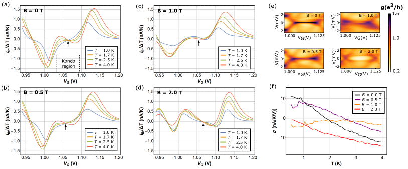
Figure 4: (a)–(d) Measured $I_{th}$ normalized by $\Delta T$ for different $T$ as indicated in the figure. The black arrows indicate $V_{G}$ positions around which the values of $\sigma$ in (f) are determined. The magnetic field is increased from $B=0$ to $B=2$ T from (a)–(d) as indicated in the figures. The dashed lines in (a) indicate the $V_{G}$ range that corresponds to the Kondo regime. (e) Charge stability diagrams showing $g$ as a function of $V$ and $V_{G}$, measured at the base temperature $T_{0}<100$ mK for values of $B$ corresponding to those used in (a)–(d). (f) Thermocurrent slope, $\sigma=(dI_{th}/dV_{G})/\Delta T$, as a function of $T$ at $B$ field values corresponding to those used in (a)–(d).

We now turn our attention to the thermoelectric properties of QDs in the Kondo regime. The $T=4$ K trace in Fig. 2(c) illustrates the expected behavior of $I_{th}(V_{G})/\Delta T$ in the absence of Kondo correlations, where it undergoes twice as many sign reversals as there are charge degeneracy points – one when passing through zero at each of the charge degeneracy points and one in the middle of every Coulomb valley Beenakker and Staring (1992); Staring et al. (1993); Dzurak et al. (1993). It was theoretically predicted in Ref. Costi and Zlatic (2010) that this behavior is qualitatively different in the presence of Kondo correlations, which cause the zero crossings at the degeneracy points to disappear. Our experimental data verifies this prediction as the two sign reversals in the gate range between $V_{G}=1.02$ and $1.10$ V disappear at low $T$. Two additional Kondo resonances are also seen in Fig. 2 (close to $V_{G}=0.9$ and $1.4$ V) but because $T_{K}$ is lower in those cases the sign reversal is not observed in Fig. 2(c).

Figure 4 shows the sign reversal of $I_{th}$ more closely and focuses on the effects of increasing $T$ and $B$. Both are known to destroy Kondo correlations and it is therefore intuitive that also the sign reversal should be affected. We aim to quantify the values of $B$ and $T$ below which the Kondo-induced sign reversal takes place. Figures 4(a)–(d) show data at different $B$ values, each for several different $T$. The corresponding charge stability diagrams for the same values of $B$ are displayed in Fig. 4(e). The sign reversal of $I_{th}$ as a function of $T$ is best seen in Fig. 4(a) where $B=0$ T. The trace at $T=1~{}\mathrm{K}\approx T_{K}$ shows a single zero-crossing within the Coulomb valley marked as the ”Kondo region”. By raising the temperature $T>T_{K}$ the two additional zero-crossings are recovered, indicating a reversal of the direction of $I_{th}$ within the Kondo region. This observation is a clear verification of theoretical predictions in Ref. Costi and Zlatic (2010).

Based on the splitting of the Kondo peak, observable in Fig. 4(e), we estimate the electron g-factor $|g_{Z}|\approx 9$ SM . Thus, $T_{K}\approx 1$ K corresponds to $B\approx 0.17$ T. Interestingly, however, the behavior of $I_{th}$ at $B=0.5$ T, as shown in Fig. 4(b), remains qualitatively and quantitatively similar to the zero field case. Only when increasing $B$ to 1.0 T and 2.0 T the two additional zero-crossings are recovered at all accessible $T$ [see Figs. 4(c) and (d)].

Closer examination of the sign reversal requires analysis of the small $I_{th}$ within the Coulomb valley which is sensitive to the experimental uncertainties in the applied electrical bias ($\delta V\approx\pm 1$ $\mu$V). We therefore fit the gate-slope of the thermocurrent, $(dI_{th}/dV_{G})/\Delta T=\sigma$, at the center of the Coulomb valley [marked by arrows in Figs. 4(a)–(d)] and use its sign as an alternative indicator for the sign reversal of $I_{th}$. Figure 4(f) shows $\sigma(T)$ measured at different $B$ values. We let $T_{1}$ denote the temperature at which $\sigma(T)$ changes from positive to negative. Interestingly, we find that $T_{1}$ is larger at $B=0.5$ T ($T_{1}\approx 2.5$ K) than at $B=0$ T ($T_{1}\approx 1.8$ K), however this result does not seem to be reproduced in other devices and we do not have an explanation for it. In contrast, at field values $B=1.0$ T and $B=2.0$ T $\sigma$ no longer reverses sign as a function of $T$. Therefore, we conclude that the crossover happens between $B=0.5$ T and $B=1.0$ T. These field values correspond to $|g_{Z}|\mu_{B}B/k_{B}\approx 3T_{K}-6T_{K}$, which is consistent with measurements under $B$ field on other devices SM .

Table 1 summarizes our results from all devices, see SM SM for the corresponding data and analysis. We estimate the relative errors for $U$ and $T_{K}$ to be in the range $\pm 10\%$, which translates into a similar error for $\Gamma$. The accuracy of $T_{1}$ depends mostly on the accuracy of the thermometry, which we have not been able to quantify. However, we do not expect it to be a source of significant error. For all resonances we find $T_{1}/T_{K}\approx 1.2-1.8$. This is in good quantitative agreement with theory predictions in Ref. Costi and Zlatic (2010) where $T_{1}/T_{K}\approx 1.6$ for $U/\Gamma=3$.

Table 1: Summary of data from several devices. QD1a (in bold) represents results obtained on the device QD1 for which the data is shown in this Letter. QD1b represents results obtained on the same device QD1 but in a different $V_{G}$ range. QD2 and QD3 represents results obtained on devices QD2 and QD3.

	$U$(meV)	$T_{K}$(K)	$\Gamma$(meV)	$T_{1}$(K)
QD1a	3.5	1.0	1.1	1.8
QD1b	2.2	0.6	0.7	0.7
QD2	2.6	0.6	0.8	0.8
QD3	3.0	0.8	1.0	1.2

In conclusion, we have presented a detailed experimental study of the thermoelectric properties of Kondo correlated QDs. Our measurements confirm the theoretical prediction Costi and Zlatic (2010) that sufficiently strong Kondo correlations can reverse the direction of $I_{th}$ over a finite range in $V_{G}$. We find quantitative agreement with theoretical predictions for the temperature $T_{1}$ at which sign the reversal takes place. We have also investigated the magnetic field dependence of $I_{th}$ and conclude that, unlike other transport quantities which change behavior at $|g_{Z}|\mu_{B}B/(k_{B}T_{K})\approx 1$ Filippone et al. (2018), the sign reversal of $I_{th}$ remains until this ratio is significantly larger than 1. This raises new questions and opens up for further theoretical and experimental studies. More generally, our work demonstrates that the use of thermoelectric measurements can be a sensitive probe of Kondo physics and other strong correlation effects. An interesting direction for future works is to investigate more complex QDs with additional symmetries Karki and Kiselev (2017) or the nonlinear, large $\Delta T$, regime Sierra et al. (2017); Dorda et al. (2016), where theoretical predictions are much more challenging.