Biased random walks with finite mean first passage time

Abstract

A power-law distance-dependent biased random walk model with a tuning parameter ($\sigma$) is introduced in which finite mean first passage times are realizable if $\sigma$ is less than a critical value $\sigma_{c}$. We perform numerical simulations in $1$-dimension to obtain $\sigma_{c}\sim 1.14$. The three-dimensional version of this model is related to the phenomenon of chemotaxis. Diffusiophoretic theory supplemented with coarse-grained simulations establish the connection with the specific value of $\sigma=2$ as a consequence of in-built solvent diffusion. A variant of the one-dimensional power-law model is found to be applicable in the context of a stock investor devising a strategy for extricating their portfolio out of loss.

I Introduction

In a variety of stochastic phenomena, it is of interest to track when a random process first reaches a threshold value Redner (2001); Weiss (1981); Bar-Haim and Klafter (1998); Bray et al. (2013). This is called first passage. For example, the decision to buy or sell stock is made depending on when the fluctuating stock price reaches a particular level for the first time. Another example is the diffusion of a particle in the presence of an absorbing boundary such that the diffusion stops the first time the particle reaches the absorbing boundary Chandrasekhar (1943). First passage properties of random walks have applications in various fields of science including physics Montroll (1969), finance Jiang and Pistorius (2008), ecology Fauchald and Tveraa (2003) and chemistry Kim (1958).

For unbiased random walks in one-dimensional space, it can be shown that with probability unity, first passage will occur, although the mean first-passage time is infinite Tracy . It would be of interest to understand whether and in what proportion the introduction of bias can result in a finite expectation value of the mean first-passage time. The exploration of this question in the context of a particular type of bias, namely power-law bias is the central objective of this paper. We introduce a one-parameter $(\sigma)$ power-law distance-dependent biased random walk model in which the expectation value of the first-passage time is found to be finite when $\sigma$ is less than a critical value.

Distance-dependent biased stochastic motion is in fact, a ubiquitous phenomenon in nature. Bacterial motion is one such example where the bacterium moves towards food or away from toxin respectively, by the mechanism of chemotaxis Berg (1993). Another example where such biased random walk is observed is in the biochemical cycle of molecular motors Thomas et al. (2001). This process at the simplest level can be compared to a biased random walk in which the bias is dependent on the position of the random walk at every instant. In this paper, we make a connection between chemotaxis and the power-law biased random walk model introduced above. To do this, we perform coarse-grained simulations for a pair of small colloidal particles, one of which is a source of chemical reaction and the other chemotaxes towards it by diffusiophoresis.

If the movement of stock is well-modeled by an unbiased random walk, the implication for an investor awaiting the price to hit a particular value is that they can be certain this will happen, but they may have to wait forever. Since this is an unsatisfactory situation to be in, the possibility of controlled bias to make the expected first-passage time finite would be greatly desirable. A variant of the power-law bias model which could potentially be applied in such a realistic stock market investing scenario is therefore introduced and studied. Here, the external bias comes naturally from the buying of stock intermittently, and the number of stock purchased is tuned according to the power-law model. The finite expectation value of first-passage time could potentially be exploited as an active strategy by an investor with sufficient surplus funds to extricate a loss-making stock out of loss.

The organization of this paper is as follows. In the next section, we review the first-passage properties of unbiased random walks, and random walks with a constant bias. The third section introduces the power-law bias model, and some novel simulation techniques we have developed to study it, and then discusses the results. The fourth section describes in some detail the chemotaxis example supplemented with molecular simulations. The fifth section describes the variant model specially designed as a strategy for a loss-making investor, followed by simulation results. A concluding section wraps up the paper.

II Review of first passage in random walks

II.1 Unbiased case

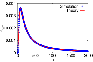
Figure 1: The first-passage probability as a function of the number of steps taken for an unbiased random walk starting from $m=16$ to the origin. The diamond symbols depict the points from the simulation. The solid line is the curve obtained from Eqn. 4.

Let $p_{n,m}$ denote the probability for a one-dimensional random walk starting at some distance $m>0$ from the origin to be at the origin at the $n^{\text{th}}$ step.

$$p_{n,m}=\frac{1}{2^{n}}\frac{(n)!}{\left(\frac{n+m}{2}\right)!\left(\frac{n-m}{2}\right)!}=\frac{1}{2^{n}}\binom{n}{\frac{n+m}{2}}$$ (1)

since the total number of possible paths in $n$ steps is $2^{n}$ out of which $\binom{n}{\frac{n+m}{2}}$ paths reach the origin after $n$ steps. We consider the probability for the random walk to reach the origin for the first time after $n$ steps, i.e., the first-passage probability to the origin denoted by $f_{n,m}$.

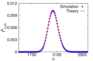
Figure 2: The first-passage probability as a function of the number of steps taken for a biased random walk with $p-q=0.5$ starting from $m=1024$ to the origin. The diamond symbols depict the points from the simulation. The solid line is the curve obtained from Eqn. 7.

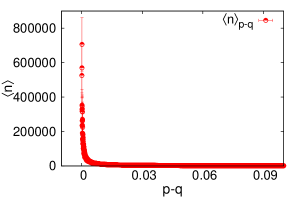
Figure 3: The plot shows the simulation results of the mean first-passage time $\langle n\rangle_{p-q}$ to the origin for a sample of 500 random walks starting from $m=100$ with a constant bias of $p-q=0$ to $p-q=0.1$ towards the origin. High error-bars for $p-q=0$ is indicative of infinite mean first-passage time.

Here, we assume that either $m$ and $n$ are both even or both odd, because otherwise the random walk cannot be at the origin at the $n^{\text{th}}$ step. The number of paths from $m$ reaching the origin for the first time at the $n^{\text{th}}$ step is $\frac{m}{n}\binom{n}{\frac{n+m}{2}}$ Feller (2008). Thus, the first-passage probability to the origin for a random walk starting at $m$ is

$$f_{n,m}=\frac{1}{2^{n}}\frac{m}{n}\binom{n}{\frac{n+m}{2}}=\frac{m}{n}p_{n,m}.$$ (2)

The binomial distribution of $p_{n,m}$ is approximated by the Gaussian distribution for large $n$. We have $p_{n,m}=\frac{1}{2^{n}}\frac{(n)!}{\left(\frac{n+m}{2}\right)!\left(\frac{n-m}{2}\right)!}$. In the limit of large $n$, using Stirling’s formula, $\ln{(n!)}=(n+\frac{1}{2})\ln{n}-n+\frac{1}{2}\ln{2\pi}+O(n^{-1})$, where $O(n^{-1})\rightarrow 0$ as $n\rightarrow\infty$, and the series expansion $\ln{\left(1\pm\frac{m}{n}\right)}=\pm\frac{m}{n}-\frac{m^{2}}{2n^{2}}+O(m^{3}/n^{3})$, we find that when $n\rightarrow\infty$ and $m\ll n$, $\ln{p_{n,m}}\simeq-\frac{1}{2}\ln{n}+\ln{2}-\frac{1}{2}\ln{2\pi}-m^{2}/2n$. Thus, the asymptotic formula is

$$p_{n,m}=\left(\frac{2}{\pi n}\right)^{\frac{1}{2}}\exp(-m^{2}/2n).$$ (3)

So for large $n$, the first-passage probability to the origin at the $n^{\text{th}}$ step for a random walk starting at $m$ is given by

$$f_{n,m}=\frac{m}{n}\left(\frac{2}{\pi n}\right)^{\frac{1}{2}}\exp(-m^{2}/2n).$$ (4)

We find that the simulation agrees with this equation for $f_{n,m}$ as seen in Fig. 1.

The first-passage probability to an absorbing point may be found by comparing the random walk to diffusion Redner (2001). In continuous space and time, the first-passage probability to the origin (absorbing point) for a random walk starting at $x_{0}$ at time $t$ is

$$F(0,t)=\frac{x_{0}}{\sqrt{4\pi Dt^{3}}}e^{-x_{0}^{2}/4Dt}.$$ (5)

We can see that $\int\limits_{0}^{\infty}F(0,t)dt=1$ which means the random walk or diffusing particle is sure to reach the absorbing point eventually.

Although the random walk is sure to reach the origin, the mean time for the first-passage to the origin is infinite. The average time required by a random walk starting from $m$ to reach the origin for the first time is its mean first-passage time to the origin. It is given by $\langle n\rangle=\sum\limits_{n=0}^{\infty}nf_{n,m}$. For the unbiased random walk, it follows from Eqn. 4 that as $n\rightarrow\infty$, $f(n,m)\sim\frac{1}{n^{\frac{3}{2}}}$ and the mean first-passage time, $\langle n\rangle=\sum\limits_{n=0}^{\infty}nf_{n,m}\sim\sum\limits_{n=0}^{\infty}\frac{1}{\sqrt{n}}\rightarrow\infty$. Thus, the mean time for the unbiased random walk to reach the origin for the first time is infinite.

II.2 Constant bias case

We now consider a random walk starting at $m>0$ for which the probability of taking a step towards the origin is $p$ and the probability of taking a step in the opposite (positive) direction is $q$, where $p+q=1$. Here, the constant bias or drift towards the origin is $p-q$. In order to find the first-passage probability to the origin at the $n^{\text{th}}$ step for such a random walk, the number of paths is the same as in the unbiased case, i.e., $\frac{m}{n}\binom{n}{\frac{n+m}{2}}$. Thus, for the biased case, the first-passage probability is given by

$$f^{b}_{n,m}=\frac{m}{n}p^{\frac{n+m}{2}}q^{\frac{n-m}{2}}\binom{n}{\frac{n+m}{2}}=\frac{m}{n}p^{b}_{n,m},$$ (6)

since $\frac{n+m}{2}$ steps are taken towards the origin and $\frac{n-m}{2}$ steps in the positive direction. For large $n$, we approximate this binomial distribution by the Gaussian distribution that is centred about the mean Haber (2012), which is now displaced from the origin. Thus, for large $n$, the first-passage probability to the origin for such a biased random walk starting from $m$ is

$$f^{b}_{n,m}=\frac{m}{n}\sqrt{\frac{1}{2\pi npq}}e^{-(m-n(p-q))^{2}/2(4npq)}.$$ (7)

In Fig. 3, the graph of $f^{b}_{n,m}$ obtained by simulation is compared with the curve from Eqn. 7.

When $p-q>0$, the mean first-passage time $\langle n\rangle$ is finite but when $p=q=0.5$, it reduces to the unbiased case and $\langle n\rangle$ is infinite. Fig. 3 compiles data from a simulation. It is seen that for $p-q=0$, the mean first-passage time $\langle n\rangle$ shoots up with high error bars whereas for $p-q>0$, the error bars are small. The high error bars show that the average time taken will not approach a limit if the sample size is increased implying that the mean first-passage time is infinite.

III Power-law biased random walk

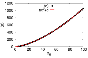
Figure 4: Variation of the mean first-passage time $\langle n\rangle$ with the initial distance from the origin $x_{0}$ for $\sigma=0.6$. A fit for the graph with the function $ax^{b}+c$ gives $a=0.750\pm 0.001$, $b=1.574\pm 0.0003$ and $c=1.228\pm 0.076$. The exponent $b$ is close to $\sigma+1$.

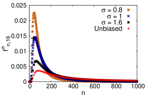
Figure 5: First-passage probability as a function of the number of steps in one dimension for different values of $\sigma$ and initial distance from the origin $x_{0}=16$. As $\sigma$ is decreased, we see that the large $n$ tails of the probability curves become steeper.

III.1 Model

Although a constant bias in a random walk yields finite mean first-passage time, the cost of a constant driving force is very high and unlikely to be seen in natural systems. Here, we introduce a one-parameter $(\sigma)$ power-law distance-dependent biased random walk model to attain finite mean first-passage time. The model is inspired from chemotaxis, in which a living cell experiences a distance-dependent drift towards a target in response to a chemical gradient produced by the target Wikipedia contributors (2018). We consider the origin to be the location of the target and design the bias towards it to vary with the position of the random walk $x$ as $\frac{1}{{x}^{\sigma}}$ where $\sigma>0$. The average time taken to get the fixed target captured by the diffusing cell or particle corresponds to the mean first-passage time of the random walk to the origin. We investigate how the mean first-passage time to the fixed target varies with $\sigma$.

In one-dimensional space, the biased random walk starting from $x_{0}>0$ operates according to the following rule. At each step, the random walk has a probability $p=\frac{1}{2}+\frac{1}{2x^{\sigma}}$ to take a step towards the origin and a probability $q=\frac{1}{2}-\frac{1}{2x^{\sigma}}$ to take a step in the positive direction away from the origin, where $x$ is the location of the random walk at the current step. The driving force in the random walk gives it a drift velocity $\frac{dx}{dt}=p-q=\frac{1}{x^{\sigma}}$ towards the origin. From a rough calculation of the mean first-passage time to the origin: $\langle n\rangle\sim\int tdt\sim|\int\limits_{x_{0}}^{0}x^{\sigma}dx|$, we deduce that the mean first-passage time $\langle n\rangle\sim{x_{0}}^{\sigma+1}$. Support for this is seen in Fig. 5 for the case $\sigma=0.6$.

In this model, $\sigma$ decides the strength of the bias towards the target and on varying $\sigma$ we find that the mean first-passage time to the origin becomes finite below a critical value $\sigma_{c}$. This is evident from our simulations in two ways. Firstly, Fig. 5 shows the plots obtained for the first-passage probability for random walks starting from $x_{0}=16$ for different values of $\sigma$. As the bias is increased, the large $n$ tail of $f^{\sigma}_{n,x_{0}}$ becomes steeper. We saw in the unbiased case that $f_{n,m}\sim\frac{1}{n^{\frac{3}{2}}}$ as $n\rightarrow\infty$. If we posit that for our model, $f_{n,x_{0}}^{\sigma}\sim\frac{1}{n^{\alpha}}$ for large $n$, the mean first-passage time $\langle n\rangle\sim\sum\limits_{n=0}^{\infty}\frac{1}{n^{\alpha-1}}$. This series is convergent if $\alpha-1>1$ and divergent if $\alpha-1\leq 1$. Thus, if the bias is strong enough, i.e., if $\sigma$ is sufficiently small, we may have $\alpha>2$ and finite mean first-passage time. In other words, there occurs a critical value $\sigma_{c}$ below which the weighted average of the probability curve becomes finite. Secondly, in Fig. 7 which shows results of simulations of an ensemble of random walks, large error-bars in the mean first-passage time after a certain value of $\sigma$ indicates a transition from finite to infinite mean first-passage time in the sense that the error-bars would not shrink if the sample size is increased Tracy . This transition seems to occur near $\sigma_{c}\approx 1.1$ for random walks starting from $x_{0}=100$. In the unbiased case, the large $n$ behaviour of first-passage probability is independent of the starting distance $x_{0}$. Therefore, we expect that the critical value $\sigma_{c}$ is also independent of $x_{0}$.

III.2 Simulation

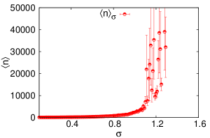
Figure 6: The plot shows the simulation results of the mean first-passage time $\langle n\rangle_{\sigma}$ to the origin for a sample of 1000 random walks starting from $x_{0}=100$ for different values of $\sigma$. High error-bars after a critical value of $\sigma$ is indicative of infinite mean first-passage time.

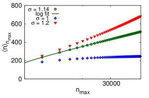
Figure 7: $\langle n\rangle_{n_{\text{max}}}=\sum\limits_{n=0}^{n_{\text{max}}}nf_{n,x_{0}}$ as a function of $n_{\text{max}}$ for different values of $\sigma$ for an initial distance from the origin $x_{0}=16$. We find that the logarithmic fit works well for $\sigma=1.14$ indicating $\sigma_{c}\approx 1.14$.

Here we describe the simulation technique used to obtain the curves of first-passage probability with respect to the number of steps as shown in Fig. 1, Fig. 3 and Fig. 5. As a concrete example, consider an unbiased one-dimensional random walk starting from $x_{0}=4$. To obtain the first-passage probability to the origin as a function of the number of steps, we take a one-dimensional array of size $x_{0}+n_{\text{max}}$ and initialize the $4^{\text{th}}$ array element with $1$ and all other array elements with $0$. This corresponds to the probability of the random walk being at $x_{0}=4$ to be equal to $1$ initially. At the next step, the probability distributes itself equally to its two nearest neighbours, since the random walk can move to the left or to the right with equal probability. This is continued at each step as shown in Table 1.

	$x=0$	$x=1$	$x=2$	$x=3$	$x=4$	$x=5$	$x=6$	$x=7$
$n=0$	$0$	$0$	$0$	$0$	$1$	$0$	$0$	$0$
$n=1$	$0$	$0$	$0$	$0.5$	$0$	$0.5$	$0$	$0$
$n=2$	$0$	$0$	$0.25$	$0$	$0.5$	$0$	$0.25$	$0$
$n=3$	$0$	$0.125$	$0$	$0.375$	$0$	$0.375$	$0$	$0.125$

Table 1: An illustration of the simulation technique.

To obtain the first-passage probability at each step, the value accumulated at the $0^{\text{th}}$ array element at each step is plotted with respect to the number of steps taken. The $0^{\text{th}}$ element is reset to zero after every step, because that fraction of an infinite number of random walks have already reached the origin for the first time and cannot have another first-passage to the origin. For the random walk with the power-law bias the same simulation method can be employed. In this case, the splitting of probability at each step will not be equal but will be distance-dependent. For instance, at the first step, the probability distributes as $\frac{1}{2}+\frac{1}{2x_{0}^{\sigma}}$ and $\frac{1}{2}-\frac{1}{2x_{0}^{\sigma}}$ to the left and right neighbours respectively. By this technique, numerically exact first-passage probability at the $n^{\text{th}}$ time step can be found for different $\sigma$ but it is exact only up to finite time $n_{\text{max}}$.

We make a better estimate of $\sigma_{c}$ using the exact first-passage probability curves obtained from this simulation technique. The mean first-passage time is given by $\langle n\rangle=\sum\limits_{n=0}^{\infty}nf_{n,x_{0}}$. Since we know the exact value of $f_{n,x_{0}}$ only up to a maximum number of steps $n_{\text{max}}$, we study the dependence of $\langle n\rangle_{n_{\text{max}}}=\sum\limits_{n=0}^{n_{\text{max}}}nf_{n,x_{0}}$ on $n_{\text{max}}$. This quantity should diverge for $\sigma>\sigma_{c}$ and approach a constant value for $\sigma<\sigma_{c}$. Since we posit that $f^{\sigma}_{n,x_{0}}\sim\frac{1}{n^{\alpha}}$ in the long-time limit, at the critical value $\sigma_{c}$, $\langle n\rangle_{n_{\text{max}}}=\sum\limits_{n=0}^{n_{\text{max}}}nf^{\sigma}_{n,x_{0}}\sim\int\limits^{n_{\text{max}}}\frac{n}{n^{\alpha}}dn\sim\log{n_{\text{max}}}$.

In Fig. 7, we see that $\langle n\rangle_{n_{\text{max}}}$ appears to diverge for larger $\sigma$ and approach a constant value for smaller $\sigma$. By curve fitting we see that the logarithmic fit works excellently for $\sigma=1.14$ from which we deduce the critical value $\sigma_{c}\approx 1.14$.

IV Chemotaxis as an example of biased random walk

Chemotaxis is the movement of a particle in response to a chemical gradient present in the environment by a biased random walk. Classically the microscopic chemotaxis was studied mostly in the context of biological systems  Adler (1966); Alon et al. (1999); Berg (2004). However, recent studies have explored this process for synthetic colloidal particles Hong et al. (2007); Deprez and de Buyl (2017), that has the potential applications in the area of targeted particle delivery, microfluidics etc. To establish a connection between the colloidal chemotaxis and biased random walk, here we study the dynamics of a pair of small colloidal particles using hybrid Molecular Dynamics - Multiparticle Collision Dynamics (MD-MPCD). Among the two colloids, one is chemically active stationary target (T), while the other is a biased random walker (W) which moves towards the target (T) using the mechanism of diffusiophoresis Anderson (1989). It is the combination of diffusiophoresis and thermal fluctuations that makes W exhibit chemotaxis or biased random walk toward T.

IV.1 Walker (W) velocity using diffusiophoretic theory

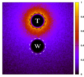
Figure 8: Formation of inhomogeneous concentration field around the the walker (W) due to the chemical reaction that converts species $A$ (fuel) to $B$ (product) in the reaction, $A+T\rightarrow B+T$ on the target (T) sphere. The walker W moves by the diffusiophoretic mechanisms due to the asymmetry of the concentration field in its vicinity.

Here, we consider a catalytically active stationary T sphere with radius $R_{1}$, that converts the species $A$ (fuel) to species $B$ (product) by irreversible chemical reaction $A+T\rightarrow B+T$ on it. The W sphere with radius $R_{2}$ is catalytically inactive and is separated from the target by an initial distance $R_{0}$ in three-dimensional space. In such a configuration, the chemical reaction on the T sphere, will generate a concentration gradient in the system, as shown in Fig. 8, which will induce a body force on W due to different interaction potentials ($V_{W,A}\neq V_{W,B}$) of these species with the walker. Such body force leads to the diffusiophoretic movement of the colloidal walker with a mean velocity component along the line of centers between the two spheres due to the axial symmetry of the system. Below we describe the analytical method to estimate the walker (W) velocity using diffusiophoretic theory  Anderson (1986).

The walker moving in a chemical gradient will experience an inhomogeneous distribution of $B$ particles in its vicinity. The interaction of the fuel ($A$) and product ($B$) particles with the surface of the walker will rise to body forces, which, because of momentum conservation will lead to a pressure and velocity gradient within the boundary layer around the walker. As a result a fluid slip velocity $v_{s}$ will be generated around the boundary layer given by the following expression Golestanian et al. (2007):

$$v_{s}=-\frac{k_{\beta}T}{\eta}(\nabla C_{B})\Lambda,$$ (8)

where $\eta$ is the viscosity of solution, $C_{B}$ is the concentration of product molecules on the outer edge of the boundary layer, and $\Lambda$ estimates the strength of interaction between the solute molecules and the surface of the colloid. The velocity of colloid can be calculated by averaging the slip velocity over the entire surface $\varsigma$ of the colloidal particle and can be given as Sarkar et al. (2014); Reigh et al.

$$V=-<v_{s}>_{\varsigma}.$$ (9)

By solving the diffusion equation $D\nabla^{2}C_{A}(r)=0$ with help of radiation boundary condition $\kappa_{0}C_{A}(R_{1},t)=\kappa_{D}R_{1}\hat{r}.\nabla{C_{A}}(R_{1},t)$, the concentration field of fuel and product particles can be achieved. Here $R_{1}$ is the radius at which reaction takes place and $C_{A}(r\rightarrow\infty)=C_{0}$ for continuous fuel supply at the boundaries to maintain the steady-state. $C_{A}+C_{B}=C_{0}$, $D$ is the diffusion coefficient of the solute particles, $k_{D}=4\pi R_{1}D$ is Smoluchowski rate constant and $\kappa_{0}$ is intrinsic reaction rate constant. By solving the diffusion equation, concentration field of product particles can be given as

$$C_{B}(r)=\frac{\kappa_{0}C_{0}}{\kappa_{0}+\kappa_{D}}\frac{R_{1}}{r}.$$ (10)

At any time instant $t$, let ${\bf{R}}(t)$ be the vector distance from W to T. Then the instantaneous velocity of W sphere can be calculated by averaging the gradient of product concentration over the outer edge of W sphere which has radius $R_{2}$. By averaging the gradient over the outer edge and projecting velocity of W sphere along the direction of ${\bf{R}}(t)$, $V_{z}(t)=\hat{\bf{R}}(t).{\bf{V}}(t)$ Sarkar et al. (2014); Rückner and Kapral (2007).

$$V_{z}(t)=\frac{2k_{B}TC_{0}\Lambda}{3\eta}\frac{k_{0}}{k_{0}+k_{D}}\frac{R_{1}}{R(t)^{2}}\equiv\frac{\lambda}{R(t)^{2}},$$ (11)

where $\Lambda=\int_{0}^{\infty}dr\>r(e^{-\beta V_{B}(r)-e^{-\beta V_{A}(r)}})$.

Further, the time evolution of separation between the spheres can be obtained by integrating Eqn. 11. We find $R(t)=[R_{0}^{3}-3\lambda t]^{1/3}$, where $R_{0}$ is the initial separation between the spheres. Thus the time taken by the walker to reach the encounter distance $R_{f}=R_{1}+R_{2}$ is given by

$$\tau=\frac{(R_{0}^{3}-R_{f}^{3})}{3\lambda}.$$ (12)

IV.2 Microscopic dynamics

The microscopic dynamics is a coarse-grain dynamics where molecular dynamics (MD) is combined with multiparticle collision (MPC) dynamics  foo . In this scheme, fluid is modelled by $N_{sol}$ point like particles with mass $m_{s}$ having the positions ${\bm{r}}_{i}$ and velocities $\bm{v}_{i}$. The interaction between the fluid particles is governed by multiparticle collision (MPC), whereas the interaction between colloids and fluid particle is through MD. MPC dynamics has two steps: streaming and collision. In the streaming step the dynamics is evolved by Newton’s equation of motion. In the collision step, all the fluid particles are sorted into small cubic cells of length $a$, which is larger than the mean free path. In every collision step the relative velocity of fluid particles is rotated around a randomly chosen axis by an angle $\phi$ with respect to the center of mass velocity of every cell. The velocity of $i^{\text{th}}$ fluid particle after collision is ${\bm{v}_{i}}^{{}^{\prime}}=\bm{v}_{cm}+\bm{\omega}(\phi)(\bm{v}_{i}-{\bm{v}}_{cm})$, where $\bm{v_{cm}}$ is the center-of-mass velocity of fluid particles in a cell, and $\bm{\omega}$ is a rotation matrix. To ensure Galilean invariance, a random shift is being given to the collision cells Ihle and Kroll (2001). The dynamical method described above conserves mass, momentum and energy locally.

The colloids (T and W) interact with fluid particles through repulsive Lennard-Jones (LJ) potential $V=4\epsilon[\left(\rho/r\right)^{12}-\left(\rho/r\right)^{6}+(1/4)]$ within the cutoff $r_{c}=2^{(1/6)}\rho$. Here $\epsilon$ and $\rho$ are energy and distance parameters respectively. In addition, repulsive LJ potential is included to take care of the excluded volume interaction between the colloids. To include the diffusiophoretic effects for W motion, we choose the interaction of fuel and product particles with W colloid different $(\epsilon_{A}>\epsilon_{B})$. This specific choice of energy parameters is to ensure the motion of W colloid towards T. To generate the products around colloids an irreversible chemical reaction $A\rightarrow B$ takes place on the surface of T. Further, to maintain the system in steady state, the product particles are converted back to the fuel when they are diffused far from the colloids.

In the simulation, all quantities are reported in dimensionless units. Length, energy, mass and time are measured in the units of MPC cell length a, $\epsilon$, fluid mass $m_{s}$ and $a\sqrt{m_{s}/\epsilon}$ respectively. Dimension of cubic box is $L=50$. The MPC rotation angle by which the velocities being rotated about a randomly chosen axis is fixed at $\phi=120^{\circ}$. The collision time step $\tau=0.1$. The average fluid particles density in a MPC cell $c_{0}$=10. The system temparature is fixed at $\kappa_{B}T=1$. MD time step $\Delta t=0.01$. The energy parameters for W interaction are chosen as $\epsilon_{A}=1.0$ , $\epsilon_{B}=0.1$ for fuel and product particles respectively. The effective radii of the sphere are $2^{(1/6)}\rho$, where $\rho=2$. Masses of the colloids are adjusted according to their diameters to ensure density matching with the solvent.

IV.3 Comparison of walker dynamics with power-law biased model

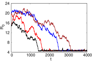
Figure 9: Plot of distance between walker and target as a function of time for different realisations. For two realisations the initial separation $R_{0}=20$, whereas for the others it is $R_{0}=15$. The time where the distance attains its minimum value is the capture time

The dynamical processes responsible for the biased random walk of the W involves diffiosiophoresis that imparts directed motion to W and the thermal fluctuations that randomises its direction. Fig. 9 shows some representative trajectories for the walker depicting the competition between the stochastic and deterministic components of the processes. The distance-dependent bias towards the target is evident here. At large distances, the W sphere exhibits mostly random displacements, whereas when the distance between W and T goes down, the directed motion dominates leading to eventual capture.

When the distance between the T and W spheres are large, the walker encounters with lesser concentration of product $B$ as the source of the product is situated at the target. This results in the Brownian motion of the W due to thermal fluctuations. As the distance between T and W decreases, the walker experiences enhanced concentrations of $B$, leading to an increased directed velocity towards the target. In the microscopic simulations we are able to probe the concentration fields responsible for the dynamics of W sphere.

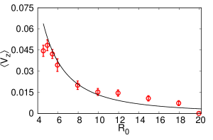
Figure 10: The velocity $V_{z}$ of walker W as a function of the separation $R_{0}$ between the W and T spheres. The solid line $R_{0}^{-2}$ fit. Averages were obtained from 80 realizations of the dynamics.

The directed velocity of the W sphere, $V_{z}$, is plotted in Fig. 10 as a function of the distance $R_{0}$ separating the centers of the two spheres. The figure shows the expected increase in velocity as the W sphere approaches the T sphere. The velocity profile exhibit a $R_{0}^{-2}$ power law behavior as predicted in the diffusiophoretic theory Eqn. 11. Fig. 10 shows an excellent agreement between the microscopic simulation and diffusiophoretic theory, except at short distance, where the velocity starts decreasing in simulations. The discrepancy between the microscopic simulations and diffusiophoretic theory at short distance may be due to the slight difference of boundary conditions in these two cases.

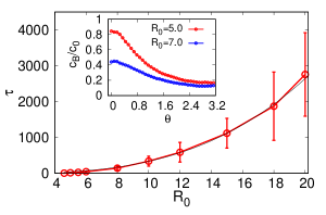
Figure 11: Capture time $\tau$ as a function of the initial separation $R_{0}$ between the spheres. The solid line is the $R_{0}^{3}$ power law fit. Inset shows the concentration field of products around W for two different initial distances $R_{0}=7.0$ and $R_{0}=10.0$. Simulation results are obtained from averages over 80 realizations.

The capture time, $\tau$ which is defined by the time taken by the W sphere, initially at a distance $R_{0}$ from the target, to reach the T sphere. Fig. 11 shows how $\tau$ varies with $R_{0}$. The capture time profile goes as $R_{0}^{3}$ power law both in diffusiophoretic theory and simulation.

The concentration and fluid velocity fields vary during the capture process, and these variations play a crucial role in determining the details of the capture mechanism. The concentration fields of $B$ species on the surface of the W sphere for two different $R_{0}$ are shown in the inset of Fig. 11. It is evident that for the larger distances between T and W, the gradient is not effective enough for W sphere to respond whereas for small distances it is prominent. Hence, the bias towards the target is enhanced at shorter distances, giving rise to reduced capture time.

Hence, the above model for chemotaxis using a pair of colloidal spheres is a realization of a particular case of the power-law biased random walker model described earlier, with $\sigma=2$ in three dimensions. A quantitative mapping of the results from the two sections is not part of the scope of the present effort. However, the strong agreement between the exponents depicted in Fig. 5 and Fig. 11 is testimony to the relevance of the power-law model in the chemotaxis context. Fig. 5 corresponds to $\sigma=0.6$ which lies below the critical value (in one dimension), and therefore the mean first passage times are observable within the simulation time scale. Fig. 11, on the other hand corresponds to $\sigma=2$, which may well be above the critical value of the power-law model in three dimension, and yet the timescales are within measurable limits. The reason for this could be that the natural lengthscales and timescales in the two problems are quite different. As the radius of the walker is shrunk, we found that the capture times became immeasurably large, perhaps indicative that $\sigma=2$ lies above the critical value in three dimensions.

The power-law model may prove to be a useful generalization also for chemotaxis, if an appropriate technique to tweak the exponent may be engineered. We can envisage applications where it is desirable to bring down the exponent below the critical value so that really tiny capture times may be achieved. One method by which this could be accomplished is to introduce some type of disorder or crowding Rajesh and Majumdar (2001), which should make the motion of the solute particle sub-diffusive.

V Stock market example

Another potential application of the biased random walk could be in stock investing. We imagine a scenario where an investor has bought stock at some time in the past, and finds that its current value is in a state of loss. The investor would be interested in finding ways to speed up the first passage of the stock value back to break-even. A variant model of the power-law biased random walk introduced above may offer a strategy by which the average time taken till break-even may be shortened. The required bias may be applied here ‘by-hand’ by simply buying more stocks intermittently. In this model, an unbiased discrete random walk starting from $x_{0}>0$ makes intermittent jumps towards the origin. The distance by which the random walk jumps depends on the position $x$ of the random walk and is proportional to $\frac{1}{x^{\sigma}}$ similar to the power-law model. The starting point of the random walk $x_{0}$ is equivalent to the net amount by which a stock price has fallen after it has been bought and the origin corresponds to the break-even point.

Let $s(t)$ denote the price of a stock at time $t$ and $x(t)$ the average gain or loss at time $t$. Then $x(t)=s(t)-s_{\text{avg}}(t)$ where $s_{\text{avg}}(t)$ is the average amount spent per stock before time $t$. The position of the random walk $x$ is equivalent to the negative of $x(t)$. In case of a net loss, stocks are bought intermittently to reduce the net loss in steps. This action of reducing the net loss by buying stocks corresponds to the intermittent jumping of the random walk. The amount by which the net loss is reduced can be tuned to match the jump size in the model. This tuning is achieved by deciding the number of stocks that are bought. The jumping of the random walk or buying of stocks is carried out after every $t_{\text{watch}}$ steps as long as there is a net loss or until the random walk crosses the origin.

Suppose after $t_{\text{watch}}$ time steps, at time $t$, $x(t)<0$. Some number of stocks are bought at the price $s(t)$ so that $x(t)$ is raised to $x(t)=s(t)-s_{\text{avg}}(t)$ where $s_{\text{avg}}(t)$ is now the average amount spent per stock after buying stocks costing $s(t)$. Since we had $s(t)<s_{\text{avg}}(t)$, after buying stocks at $s(t)$, $s_{\text{avg}}(t)$ will have reduced.

If the jump size of the random walk is fixed by a constant $\gamma$ so that the jump length $\frac{\gamma}{x^{\sigma}}\equiv\frac{\gamma}{|x(t)|^{\sigma}}$, the number of stocks to be bought after every $t_{\text{watch}}$ time steps can be found. Suppose at $t=t_{0}$, $N_{0}$ stocks were bought and at $t=t_{1}$, there was a huge net loss and the process of buying stocks intermittently was started. If $N_{1}$ stocks were bought at $t_{1}$, $N_{2}$ stocks at $t_{2}=t_{1}+t_{\text{watch}}$ and similarly $N_{i-1}$ stocks were bought at $t_{i-1}=t_{1}+(i-2)t_{\text{watch}}$, we have

$$s_{\text{avg}}(t_{i})=\frac{N_{0}s(t_{0})+N_{1}s(t_{1})+\cdots+N_{i-1}s(t_{i-1})}{N_{0}+N_{1}+\cdots+N_{i-1}}$$ (13)

for the net amount spent per stock after buying stocks at $t=t_{i-1}$. The net loss has been reduced. In terms of the number of stocks bought,

$$\frac{N_{0}s(t_{0})+\cdots+N_{i-1}s(t_{i-1})}{N_{0}+\cdots+N_{i-1}}-\frac{N_{0}s(t_{0})+\cdots+N_{i}s(t_{i})}{N_{0}+\cdots+N_{i}}$$ (14)

$$=\frac{\gamma}{|x(t_{i})|^{\sigma}}.$$

Upon rearranging the left-hand side of Eqn. 14, we see that the number of stocks to be bought at $t=t_{i}$ is

$$N_{i}=(N_{0}+N_{1}+\cdots+N_{i-1})\frac{\gamma}{-x(t_{i})|x(t_{i})|^{\sigma}-\gamma}.$$ (15)

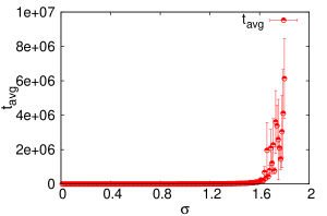
Figure 12: Mean first-passage time to the origin $t_{\text{avg}}$ for different values of $\sigma$ with $\gamma=600$, $t_{\text{watch}}=10$ and $x_{0}=500$. The high error-bars after $\sigma\sim 1.6$ is indicative of a transition from finite to infinite mean first-passage time.

In the random walk model, $x(t_{1})$ corresponds to the initial position $x_{0}$ of the unbiased random walk. The random walk makes jumps of length $\frac{\gamma}{x^{\sigma}}$ where $x\equiv|x(t)|$ at $t=t_{1}$, $t=t_{2}$ and so on until the random walk reaches the origin. The mean first-passage time to the origin is found for different values of $\sigma$ and a critical value of $\sigma$ is seen beyond which the mean first-passage time becomes arbitrarily large. This can be seen in Fig. 12 for a random walk starting from $x(0)=500$ making jumps towards the origin with $t_{\text{watch}}=10$ and $\gamma=600$. The large error bars seen for higher values of $\sigma$ indicate infinite mean first-passage time to the origin. From the plot, the critical value of $\sigma$ seems to be around $\sigma_{c}\approx 1.6$.

The constants $\gamma$ and $t_{\text{watch}}$ can be chosen in a manner to optimize the time taken to break even and to minimize the total amount that needs to be invested. The value of $\sigma$ should be chosen to lie below $\sigma_{c}$ so that the average time required to break even is expected to be finite. Of course this model relies on the assumption that the stock is performing an unbiased random walk, and the only bias comes from the investor, which is in general not true. However, the strength of this strategy lies in the identification of a critical value of the parameter $\sigma$ below which the sucess potential of the strategy is greatly enhanced.

VI Concluding Remarks

We have introduced a one-parameter distance-dependent power-law biased random walk model in which the first passage properties show dramatically different behavior depending on the value of the parameter $\sigma$. In one dimension, when the value of $\sigma$ is below a critical value $\sigma_{c}\approx 1.14$, we report a finite value of the mean first-passage time. For $\sigma>\sigma_{c}$, the motion is similar to that of the unbiased random walk, where although the probability of return is unity, the mean first-passage time is infinite. This is understood from the first-passage probability which is posited to go as $f_{n,m}\sim\frac{1}{n^{\alpha}}$, where $\alpha$ itself depends on $\sigma$. When $\sigma<\sigma_{c}$, $\alpha$ is greater than $2$, thus making the summation $\sum nf_{n,m}$ convergent, which in turn yields a finite mean first-passage time. With the help of some novel numerical techniques, we show how an exact simulation of these biased random walks becomes possible, if one restricts the study to a finite maximum time. The value of the maximum time is only limited by memory resources.

We point out that this model is closely connected to the real-world problem of chemotaxis, where distance-dependent bias arises naturally. The phenomenon of chemotaxis is well described using diffusiophoretic theory, supplemented with microscopic simulations to obtain first passage properties. It turns out that chemotaxis corresponds to the three-dimensional version of the above power-law biased random walk model with the specific parameter value of $\sigma=2$, due to the inherent diffusive nature of the solvent transport. Despite $\sigma$ being apparently larger than the critical value, finite capture times are seen in simulations. The analogy between the power-law model and chemotaxis model should be viewed with caution, because in the latter, the walker and the target are not point-particles. The finite-radii of the walker and the target ensure that a weaker bias is still effective in directed motion of the walker, and hence we see finite capture times even when $\sigma$ is apparently greater than the critical value. We have found that reducing the radii of the spheres leads to larger capture times, which after a point become inaccessible within the simulations.

The second example to which we attempt to apply our model is to the problem of a stock investor devising a strategy to extricate himself from loss. Here, we introduce a variant of the power-law biased random walk model, where on top of an unbiased random walk, we embed intermittent jumps directed towards the target, whose size is determined by the power-law. Similar to the above model, there is a critical $\sigma_{c}\sim 1.6$ below which mean first passage times are finite. More tests based on real data from stock portfolios would be desirable to explore whether this strategy may be adopted in a real-world scenario. This stock market problem is inherently one-dimensional and therefore the model is well-suited for such tests.

We anticipate that the proposed power-law biased random walk model may find application in other phenomena. It would be particularly interesting to consider higher dimensional generalizations of this model, although memory requirements would make the simulations more challenging. Incorporation of crowding and disorder effects into the chemotaxis scenario might provide a knob which can tune the underlying $\sigma$ in the model. An improvised power-law model with finite radii of the walker and target might provide an alternative route to make more quantitative connections to the chemotaxis scenario. It would be exciting if this model can provide fresh insights into stock investing strategy.