Breaking of ensemble equivalence for
perturbed Erdős-Rényi random graphs

Abstract

In [18] we analysed a simple undirected random graph subject to constraints on the densities of edges and triangles, considering the dense regime in which the number of edges per vertex is proportional to the number of vertices. We computed the specific relative entropy of the microcanonical ensemble with respect to the canonical ensemble, i.e., the relative entropy per edge in the limit as the number of vertices tends to infinity. We showed that as soon as the constraints are frustrated, i.e., do not lie on the Erdős-Rényi line (where the density of triangles is the third power of the density of edges), there is breaking of ensemble equivalence, meaning that the specific relative entropy is strictly positive. In the present paper we analyse what happens near this line. It turns out that the way in which the specific relative entropy tends to zero critically depends on whether the line is approached is from above or from below. We identify what the constrained random graph looks like in the microcanonical ensemble in the limit as the number of vertices tends to infinity.

MSC 2010: 05C80, 60K35, 82B20.
Key words: Erdős-Rényi random graph, Gibbs ensembles, breaking of ensemble equivalence, relative entropy, graphons, large deviation principle, variational representation.
Acknowledgement: The research in this paper was supported through NWO Gravitation Grant NETWORKS 024.002.003. The authors are grateful to V. Patel and H. Touchette for helpful discussions. FdH, AR and NJS are grateful for hospitality at the International Centre for Theoretical Sciences in Bangalore, India, as participants of the program on Large Deviation Theory in Statistical Physics: Recent Advances and Future Challenges running in the Fall of 2017.

1 Introduction

1.1 Background

In this paper we analyse random graphs that are subject to constraints. Statistical physics prescribes what probability distribution on the set of graphs we should choose when we want to model a given type of constraint [15]. Two important choices are:

• The microcanonical ensemble, where the constraints are hard (i.e., are satisfied by each individual graph).

• The canonical ensemble, where the constraints are soft (i.e., hold as ensemble averages, while individual graphs may violate the constraints).

For random graphs that are large but finite, the two ensembles are obviously different and, in fact, represent different empirical situations. Each ensemble represents the unique probability distribution with maximal entropy respecting the constraints. In the limit as the size of the graph diverges, the two ensembles are traditionally assumed to become equivalent as a result of the vanishing fluctuations in the soft constraints, i.e., the soft constraints are assumed to behave asymptotically like hard constraints. This assumption of ensemble equivalence is one of the cornerstones of statistical physics, but it does not hold in general. We refer to [33] for more background on this phenomenon.

In a series of papers we investigated the possible breaking of ensemble equivalence for various choices of the constraints, including the degree sequence and the total number of edges, wedges, triangles, etc. Both the sparse regime (where the number of edges per vertex remains bounded) and the dense regime (where the number of edges per vertex is of the order of the number of vertices) were considered. The effect of community structure on ensemble equivalence was investigated as well. Relevant references are [16, 17, 18, 31, 32].

In [18], for the dense regime, we considered constraints on the densities of finitely many arbitrary subgraphs. Our main result was a variational formula for $s_{\infty}=\lim_{n\to\infty}n^{-2}s_{n}$, where $n$ is the number of vertices and $s_{n}$ is the relative entropy of the microcanonical ensemble with respect to the canonical ensemble. Our analysis relied on the large deviation principle for graphons derived in [6, 10]. For the case where the constraints were on the densities of edges and triangles we found that $s_{\infty}>0$ when the constraints are frustrated.

In the sequel we will say that we are on the Erdős-Rényi line (abbreviated to ER line) when the density of triangles is equal to the third power of the density of edges, which is typical for the Erdős-Rényi random graph. We analyse the behaviour of $s_{\infty}$ when the constraints are close to but different from the ER line. Moreover, we identify what the constrained random graph looks like asymptotically in the microcanonical ensemble. It turns out that the behaviour drastically changes when the density of triangles is slightly larger, respectively, slightly smaller than that of the ER line. The microcanonical ensemble is harder to analyse than the canonical ensemble. Yet, we do not know what the constrained random graph looks like asymptotically in the canonical ensemble below the ER line.

1.2 Literature

While breaking of ensemble equivalence is a relatively new concept in the theory of random graphs, there are many studies on the asymptotic structure of random graphs. In the pioneering work [10], followed by [24], a large deviation principle for dense Erdős-Rényi random graphs was established and the asymptotic structure of constrained Erdős-Rényi random graphs was described as the solution of a variational problem. In the past few years, significant progress was made regarding sparse random graphs as well [9, 12, 25, 37]. Two further random graph models that were studied extensively are the exponential random graph model and the constrained exponential random graph model. Exponential random graphs, which are related to the canonical ensemble considered in the present paper, were analysed in [3, 8]: [3] studies mixing times of Glauber spin-flip dynamics, while [8] uses large deviation theory to derive asymptotic expressions for the partition function. In subsequent works [28, 30, 34] the behaviour of exponential random graphs was analysed in further detail, while in [36] the focus was on sparse exponential random graphs. In [14] exponential random graphs were studied in both the dense and the sparse regime, and the main conclusion was that they behave essentially like mixtures of random graphs with independent edges. In [23, 35] constrained exponential random graphs were analysed, while in [1, 2] the additional feature of directed edges was added. In [11] large deviations were used to study random graphs constrained on the degree sequence in the dense regime.

In [20, 21, 26, 29], the asymptotic structure of graphs drawn from the microcanonical ensemble was investigated for various choices of constraints on the densities of edges and triangles. The focus of [29] was on the behaviour of random graphs for values of the edge and triangle densities close to the ER line, and a rough scaling of the graph was found via a bound on the entropy function. In the present paper we extend these results by determining the precise scaling. A similar question was addressed in [26] for a constraint on the edge and triangle density close to the lower boundary curve of the admissibility region (see Fig. 2 below). In [21], through extensive numerics, the regions were determined where phase transitions in the structure of the constrained random graph occur as the densities of edges and triangles is varied. Our results rely on this numerics near the ER line, and make it mathematically precise.

1.3 Outline

The remainder of our paper is organised as follows. In Section 2 we define the two ensembles, give the definition of equivalence of ensembles in the dense regime, and recall some basic facts about graphons. An important role is played by the variational representation of $s_{\infty}$, derived in [18] when the constraints are on the total numbers of subgraphs drawn from a finite collection of subgraphs. We also recall the analysis of $s_{\infty}$ in [18] for the special case where the subgraphs are the edges and the triangles. In Section 3 we state our main theorems and propositions on the behaviour around the ER line. Proofs are given in Sections 4 and 5.

2 Definitions and preliminaries

In this section, which is largely lifted from [18], we present the definitions of the main concepts to be used in the sequel, together with some key results from prior work. Section 2.1 presents the formal definition of the two ensembles we are interested in and gives our definition of ensemble equivalence in the dense regime. Section 2.2 recalls some basic facts about graphons, while Section 2.3 recalls some basic properties of the canonical ensemble. Section 2.4 recalls the variational characterisation of ensemble equivalence when the constraint is on a finite number of subgraph densities, proven in [18]. Section 2.5 recalls the main results in [18] for the case where the constraints are on the densities of edges and triangles.

2.1 Microcanonical ensemble, canonical ensemble, relative entropy

For $n\in\mathbb{N}$, let $\mathcal{G}_{n}$ denote the set of all $2^{{n\choose 2}}$ simple undirected graphs with vertex set $\{1,\dots,n\}$. Any graph $G\in\mathcal{G}_{n}$ can be represented by a symmetric $n\times n$ matrix with elements

$$h^{G}(i,j):=\begin{cases}1\qquad\mbox{if there is an edge between vertex }i\mbox{ and vertex }j,\\ 0\qquad\mbox{otherwise.}\end{cases}$$ (2.1)

Let $\vec{C}$ denote a vector-valued function on $\mathcal{G}_{n}$. We choose a specific vector $\vec{C}^{*}$, which we assume to be graphical, i.e., realisable by at least one graph in $\mathcal{G}_{n}$. Given $\vec{C}^{*}$, the microcanonical ensemble is the probability distribution $\mathrm{P}_{\mathrm{mic}}$ on $\mathcal{G}_{n}$ with hard constraint $\vec{C}^{*}$ defined as

$$\mathrm{P}_{\mathrm{mic}}(G):=\left\{\begin{array}[]{ll}1/\Omega_{\vec{C}^{*}},&\text{if }\vec{C}(G)=\vec{C}^{*},\\ 0,&\text{otherwise},\end{array}\right.\qquad G\in\mathcal{G}_{n},$$ (2.2)

where

$$\Omega_{\vec{C}^{*}}:=|\{G\in\mathcal{G}_{n}\colon\,\vec{C}(G)=\vec{C}^{*}\}|$$ (2.3)

is the number of graphs that realise $\vec{C}^{*}$. The canonical ensemble $\mathrm{P}_{\mathrm{can}}$ is the unique probability distribution on $\mathcal{G}_{n}$ that maximises the entropy

$$S_{n}({\rm P}):=-\sum_{G\in\mathcal{G}_{n}}{\rm P}(G)\log{\rm P}(G)$$ (2.4)

subject to the soft constraint $\langle\vec{C}\rangle=\vec{C}^{*}$, where

$$\langle\vec{C}\rangle:=\sum_{G\in\mathcal{G}_{n}}\vec{C}(G)\,{\rm P}(G).$$ (2.5)

This gives the formula [19]

$$\mathrm{P}_{\mathrm{can}}(G):=\frac{1}{Z(\vec{\theta}^{*})}\,\mathrm{e}^{H(\vec{\theta}^{*},\vec{C}(G))},\qquad G\in\mathcal{G}_{n},$$ (2.6)

with

$$H(\vec{\theta}^{*},\vec{C}(G)):=\vec{\theta}^{*}\cdot\vec{C}(G),\qquad Z(\vec{\theta}^{*}\,):=\sum_{G\in\mathcal{G}_{n}}\mathrm{e}^{\vec{\theta}^{*}\cdot\hskip 2.0pt\vec{C}(G)},$$ (2.7)

denoting the Hamiltonian and the partition function, respectively. In (2.6)–(2.7) the parameter $\vec{\theta}^{*}$, which is a real-valued vector whose dimension is equal to the number of constraints, must be set to the unique value that realises $\langle\vec{C}\rangle=\vec{C}^{*}$. As a Lagrange multiplier, $\vec{\theta}^{*}$ always exists, but uniqueness is non-trivial. In the sequel we will only consider examples where the gradients of the constraints are linearly independent vectors. Consequently, the Hessian matrix of the covariances in the canonical ensemble is a positive-definite matrix, which implies uniqueness.

The relative entropy of $\mathrm{P}_{\mathrm{mic}}$ with respect to $\mathrm{P}_{\mathrm{can}}$ is defined as

$$S_{n}(\mathrm{P}_{\mathrm{mic}}\mid\mathrm{P}_{\mathrm{can}}):=\sum_{G\in\mathcal{G}_{n}}\mathrm{P}_{\mathrm{mic}}(G)\log\frac{\mathrm{P}_{\mathrm{mic}}(G)}{\mathrm{P}_{\mathrm{can}}(G)}.$$ (2.8)

For any $G_{1},G_{2}\in\mathcal{G}_{n}$, $\mathrm{P}_{\mathrm{can}}(G_{1})=\mathrm{P}_{\mathrm{can}}(G_{2})$ whenever $\vec{C}(G_{1})=\vec{C}(G_{2})$, i.e., the canonical probability is the same for all graphs with the same value of the constraint. We may therefore rewrite (2.8) as

$$S_{n}(\mathrm{P}_{\mathrm{mic}}\mid\mathrm{P}_{\mathrm{can}})=\log\frac{\mathrm{P}_{\mathrm{mic}}(G^{*})}{\mathrm{P}_{\mathrm{can}}(G^{*})},$$ (2.9)

where $G^{*}$ is any graph in $\mathcal{G}_{n}$ such that $\vec{C}(G^{*})=\vec{C}^{*}$ (recall that we assumed that $\vec{C}^{*}$ is realisable by at least one graph in $\mathcal{G}_{n}$). The removal of the sum over $\mathcal{G}_{n}$ constitutes a major simplification.

All the quantities above depend on $n$. In order not to burden the notation, we exhibit this $n$-dependence only in the symbols $\mathcal{G}_{n}$ and $S_{n}(\mathrm{P}_{\mathrm{mic}}\mid\mathrm{P}_{\mathrm{can}})$. When we pass to the limit $n\to\infty$, we need to specify how $\vec{C}(G)$, $\vec{C}^{*}$ are chosen to depend on $n$. We refer the reader to [18, Appendix A], where this issue was discussed in detail.

Definition 2.1

In the dense regime, if

$$s_{\infty}:=\lim\frac{1}{n^{2}}S_{n}(\mathrm{P}_{\mathrm{mic}}\mid\mathrm{P}_{\mathrm{can}})=0,$$ (2.10)

then $\mathrm{P}_{\mathrm{mic}}$ and $\mathrm{P}_{\mathrm{can}}$ are said to be equivalent.

Remark 2.2

In [32], which was concerned with the sparse regime, the relative entropy was divided by $n$ (the number of vertices). In the dense regime, however, it is appropriate to divide by $n^{2}$ (the order of the number of edges).

2.2 Graphons

There is a natural way to embed a simple graph on $n$ vertices in a space of functions called graphons. Let $W$ be the space of functions $h\colon\,[0,1]^{2}\to[0,1]$ such that $h(x,y)=h(y,x)$ for all $(x,y)\in[0,1]^{2}$. A finite simple graph $G$ on $n$ vertices can be represented as a graphon $h^{G}\in W$ in a natural way as (see Figure 1)

$$h^{G}(x,y):=\left\{\begin{array}[]{ll}1&\mbox{if there is an edge between vertex }\lceil{nx}\rceil\mbox{ and vertex }\lceil{ny}\rceil,\\ 0&\mbox{otherwise},\end{array}\right.$$ (2.11)

which is referred to as the empirical graphon associated with $G$.

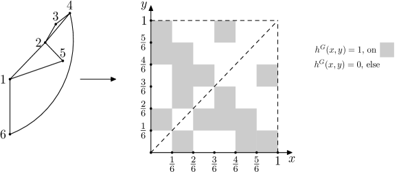
Figure 1: An example of a graph $G$ and its graphon representation $h^{G}$.

The space of graphons $W$ is endowed with the cut distance

$$d_{\square}(h_{1},h_{2}):=\sup_{S,T\subset[0,1]}\left|\int_{S\times T}\mathrm{d}x\,\mathrm{d}y\,[h_{1}(x,y)-h_{2}(x,y)]\right|,\qquad h_{1},h_{2}\in W.$$ (2.12)

On $W$ there is a natural equivalence relation $\equiv$. Let $\Sigma$ be the space of measure-preserving bijections $\sigma\colon\,[0,1]\to[0,1]$. Then $h_{1}(x,y)\equiv h_{2}(x,y)$ if $h_{1}(x,y)=h_{2}(\sigma x,\sigma y)$ for some $\sigma\in\Sigma$. This equivalence relation yields the quotient space $(\tilde{W},\delta_{\square})$, where $\delta_{\square}$ is the metric defined by

$$\delta_{\square}(\tilde{h}_{1},\tilde{h}_{2}):=\inf_{\sigma_{1},\sigma_{2}\in\Sigma}d_{\square}(h_{1}^{\sigma_{1}},h_{2}^{\sigma_{2}}),\qquad\tilde{h}_{1},\tilde{h}_{2}\in\tilde{W}.$$ (2.13)

For a more detailed description of the structure of the space $(\tilde{W},\delta_{\square})$ we refer to [4, 5, 13]. In the sequel we will deal with constraints on the edge and triangle density. In the space $W$ the edge and triangle densities of a graphon $h$ are defined by

$$T_{1}(h):=\int_{[0,1]^{2}}\mathrm{d}x_{1}\mathrm{d}x_{2}\,h(x_{1},x_{2}),\quad T_{2}(h):=\int_{[0,1]^{3}}\mathrm{d}x_{1}\mathrm{d}x_{2}\mathrm{d}x_{3}\,h(x_{1},x_{2})h(x_{2},x_{3})h(x_{3},x_{1}).$$ (2.14)

For an element $\tilde{h}$ of the quotient space $\tilde{W}$ we define the edge and triangle density by

$$T_{1}(\tilde{h})=T_{1}(h),\qquad T_{2}(\tilde{h})=T_{2}(h),$$ (2.15)

where $h$ is any representative element of the equivalence class $\tilde{h}$.

2.3 Subgraph counts

We can label the simple graphs in any order: $\{F_{k}\}_{k\in\mathbb{N}}$. Let $C_{k}(G)$ denote the number of subgraphs $F_{k}$ in $G$. In the dense regime, $C_{k}(G)$ grows like $n^{V_{k}}$ as $n\to\infty$, where $V_{k}:=|V(F_{k})|$ is the number of vertices in $F_{k}$. For $m\in\mathbb{N}$, consider the following scaled vector-valued function on $\mathcal{G}_{n}$:

$$\vec{C}(G):=\left(\frac{p(F_{k})\,C_{k}(G)}{n^{V_{k}-2}}\right)_{k=1}^{m}=n^{2}\left(\frac{p(F_{k})\,C_{k}(G)}{n^{V_{k}}}\right)_{k=1}^{m}.$$ (2.16)

The term $p(F_{k})$ counts the edge-preserving permutations of the vertices of $F_{k}$ (e.g. $2$ for an edge, $2$ for a wedge, $6$ for a triangle). The term $C_{k}(G)/n^{V_{k}}$ represents the density of $F_{k}$ in $G$. The additional $n^{2}$ guarantees that the full vector scales like $n^{2}$, in line with the scaling of the large deviation principle for graphons in the Erdős-Rényi random graph derived in [10]. For a simple graph $F_{k}$, let $\text{hom}(F_{k},G)$ be the number of homomorphisms from $F_{k}$ to $G$, and define the homomorphism density as

$$t(F_{k},G):=\frac{\text{hom}(F_{k},G)}{n^{V_{k}}}=\frac{p(F_{k})\,C_{k}(G)}{n^{V_{k}}},$$ (2.17)

which does not distinguish between permutations of the vertices. In terms of this quantity, the Hamiltonian becomes

$$H(\vec{\theta},\vec{T}(G))=n^{2}\sum_{k=1}^{m}\theta_{k}\,t(F_{k},G)=n^{2}(\vec{\theta}\cdot\vec{T}(G)),\qquad G\in\mathcal{G}_{n},$$ (2.18)

where

$$\vec{T}(G):=\left(t(F_{k},G)\right)_{k=1}^{m}.$$ (2.19)

The canonical ensemble with parameter $\vec{\theta}$ thus takes the form

$$\mathrm{P}_{\mathrm{can}}(G\mid\vec{\theta}\,):=\mathrm{e}^{n^{2}\big{[}\vec{\theta}\cdot\vec{T}(G)-\psi_{n}(\vec{\theta}\,)\big{]}},\qquad G\in\mathcal{G}_{n},$$ (2.20)

where $\psi_{n}$ replaces the partition function $Z(\vec{\theta})$:

$$\psi_{n}(\vec{\theta}):=\frac{1}{n^{2}}\log\sum_{G\in\mathcal{G}_{n}}\mathrm{e}^{n^{2}(\vec{\theta}\hskip 2.0pt\cdot\hskip 2.0pt\vec{T}(G))}=\frac{1}{n^{2}}\log Z(\vec{\theta}).$$ (2.21)

In the sequel we take $\vec{\theta}$ equal to a specific value $\vec{\theta}^{*}$ so as to meet the soft constraint, i.e.,

$$\langle\vec{T}\rangle=\sum_{G\in\mathcal{G}_{n}}\vec{T}(G)\,\mathrm{P}_{\mathrm{can}}(G)=\vec{T}^{*}.$$ (2.22)

With this choice, the canonical probability becomes

$$\mathrm{P}_{\mathrm{can}}(G)=\mathrm{P}_{\mathrm{can}}(G\mid\vec{\theta^{*}}).$$ (2.23)

Both the constraint $\vec{T}^{*}$ and the Lagrange multiplier $\vec{\theta}^{*}$ in general depend on $n$, i.e., $\vec{T}^{*}=\vec{T}^{*}_{n}$ and $\vec{\theta}^{*}=\vec{\theta}^{*}_{n}$. We consider constraints that converge when we pass to the limit $n\to\infty$, i.e.,

$$\lim_{n\to\infty}\vec{T}^{*}_{n}=\vec{T}^{*}_{\infty}.$$ (2.24)

Consequently, we expect that

$$\lim_{n\to\infty}\vec{\theta}^{*}_{n}=\vec{\theta}^{*}_{\infty}.$$ (2.25)

In the remainder of this paper we assume that (2.25) holds. If convergence fails, then we may still consider subsequential convergence. The subtleties concerning (2.25) were discussed in detail in [18, Appendix A].

2.4 Variational characterisation of ensemble equivalence

For a graphon $h\in W$ and a simple graph $F$ with vertex set $V(F)$ and edge set $E(F)$, define

$$t(F,h):=\int_{[0,1]^{|V(F)|}}\mathrm{d}x_{1}\dots\mathrm{d}x_{|V(F)|.}\prod_{\{i,j\}\in E(F)}h(x_{i},x_{j}).$$ (2.26)

Then $t(F,G)=t(F,h^{G})$, and so the expression in (2.18) can be written as

$$H(\vec{\theta},\vec{T}(G))=n^{2}\sum_{k=1}^{m}\theta_{k}\,t(F_{k},h^{G}).$$ (2.27)

The constraint $\vec{T}^{*}_{\infty}$ defines a subspace of the quotient space $\tilde{W}$,

$$\tilde{W}^{*}:=\{\tilde{h}\in\tilde{W}\colon\,\vec{T}(h)=\vec{T}^{*}_{\infty}\}.$$ (2.28)

consisting of all graphons that meet the constraint.

In order to characterise the asymptotic behavior of the two ensembles, the entropy function of a Bernoulli random variable is essential. For $u\in[0,1]$, let

$$I(u):=\tfrac{1}{2}u\log u+\tfrac{1}{2}(1-u)\log(1-u).$$ (2.29)

Extend the domain of this function to the graphon space $W$ by defining

$$I(h):=\int_{[0,1]^{2}}\mathrm{d}x\,\mathrm{d}y\,\,I(h(x,y))$$ (2.30)

(with the convention that $0\log 0:=0$). On the quotient space $(\tilde{W},\delta_{\square})$, define $I(\tilde{h})=I(h)$, where $h$ is any element of the equivalence class $\tilde{h}$. (In order to keep the notation minimal, we use $I(\cdot)$ for both (2.29) and (2.30). Below it will always be clear which of the two is being considered.) The function $\tilde{h}\mapsto I(\tilde{h})$ is well defined on the quotient space $\tilde{W}$ (see [10, Lemma 2.1]). Moreover, $\tilde{h}\mapsto I(\tilde{h})+\tfrac{1}{2}\log 2$ is the rate function of the large deviation principle in [10].

The key result in [18] is the following variational formula for $s_{\infty}$ ($\cdot$ denotes the inner product for vectors).

Theorem 2.3

[18] Subject to (2.22), (2.24) and (2.25),

$$\lim_{n\to\infty}n^{-2}S_{n}(\mathrm{P}_{\mathrm{mic}}\mid\mathrm{P}_{\mathrm{can}})=:s_{\infty}$$ (2.31)

with

$$s_{\infty}=\sup_{\tilde{h}\in\tilde{W}}\left[\vec{\theta}^{*}_{\infty}\cdot\vec{T}(\tilde{h})-I(\tilde{h})\right]-\sup_{\tilde{h}\in\tilde{W}^{*}}\left[\vec{\theta}^{*}_{\infty}\cdot\vec{T}(\tilde{h})-I(\tilde{h})\right].$$ (2.32)

Theorem 2.3 and the compactness of $\tilde{W}^{*}$ give us a variational characterisation of ensemble equivalence: $s_{\infty}=0$ if and only if at least one of the maximisers of $\vec{\theta}^{*}_{\infty}\cdot\vec{T}(\tilde{h})-I(\tilde{h})$ in $\tilde{W}$ also lies in $\tilde{W}^{*}\subset\tilde{W}$, i.e., satisfies the constraint $T^{*}_{\infty}$.

2.5 Edges and triangles

Theorem 2.3 allows us to identify examples where ensemble equivalence holds ($s_{\infty}=0$) or is broken ($s_{\infty}>0$). In [18] a detailed analysis was given for the special case where the constraint is on the densities of edges and triangles.

Theorem 2.4

[18] For the edge-triangle model, $s_{\infty}=0$ when

• $T_{2}^{*}=T_{1}^{*{3}}$,

• $0<T_{1}^{*}\leq\frac{1}{2}$ and $T_{2}^{*}=0$,

while $s_{\infty}>0$ when

• $T_{2}^{*}\neq T_{1}^{*{3}}$ and $T_{2}^{*}\geq\tfrac{1}{8}$,

• $T_{2}^{*}\neq T_{1}^{*{3}}$, $0<T_{1}^{*}\leq\tfrac{1}{2}$ and $0<T_{2}^{*}<\frac{1}{8}$,

• $(T_{1}^{*},T_{2}^{*})$ lies on the scallopy curve $($the lower blue curve Figure 2$)$.

Here, $T_{1}^{*},T_{2}^{*}$ are in fact the limits $T_{1,\infty}^{*},T_{2,\infty}^{*}$ in (2.24), but in order to keep the notation light we suppress the index $\infty$.

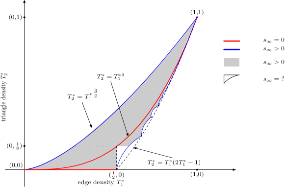
Figure 2: The admissible edge-triangle density region is the region on and between the blue curves [29].

Theorem 2.4 is illustrated in Figure 2. The region on and between the blue curves, called the admissible region, corresponds to the choices of $(T_{1}^{*},T_{2}^{*})$ that are graphical, i.e., there exists a graph with edge density $T_{1}^{*}$ and triangle density $T_{2}^{*}$. The red curves represent ensemble equivalence, while the blue curves and the grey region represent breaking of ensemble equivalence. In the white region between the red curve and the lower blue curve we do not know whether there is breaking of ensemble equivalence or not (although we expect that there is). Breaking of ensemble equivalence arises from frustration between the values of $T_{1}^{*}$ and $T_{2}^{*}$. In line with [18], by frustration we mean that these two densities do not lie on the Erdős-Rényi line.

The lower blue curve, called the scallopy curve, consists of infinitely many pieces labelled by $\ell\in\mathbb{N}\setminus\{1\}$. The $\ell$-th piece corresponds to $T_{1}^{*}\in(\frac{\ell-1}{\ell},\frac{\ell}{\ell+1}]$ and a value $T_{2}^{*}$ that is a computable but non-trivial function of $T_{1}^{*}$, explained in detail in [27, 28, 29]. The structure of the graphs drawn from the microcanonical ensemble was determined in [27, 29]. On the $\ell$-th piece:

• The vertex set can be partitioned into $\ell$ subsets. The first $\ell-1$ subsets have size $\lfloor c_{\ell}n\rfloor$, the last subset has size between $\lfloor c_{\ell}n\rfloor$ and $2\lfloor c_{\ell}n\rfloor$, with

  $$c_{\ell}:=\tfrac{1}{\ell+1}\left[1+\sqrt{1-\tfrac{\ell+1}{\ell}\,T_{1}^{*}}\,\right]\in[\tfrac{1}{\ell+1},\tfrac{1}{\ell}).$$ (2.33)

• The graph has the form of a complete $\ell$-partite graph, with some additional edges on the last subset that create no triangles within that last subset.

• The optimal graphons have the form

  $$g^{*}_{\ell}(x,y):=\left\{\begin{array}[]{ll}1,&\exists\,1\leq k<\ell\colon\,x~{}<kc_{\ell}<~{}y\mbox{ or }y<kc_{\ell}<x,\\ p_{\ell},&(\ell-1)c_{\ell}~{}<x<~{}\tfrac{1}{2}[1+(\ell-1)c_{\ell}]<y\mbox{ or }(\ell-1)c_{\ell}~{}<y<~{}\tfrac{1}{2}[1+(\ell-1)c]<x,\\ 0,&\mbox{otherwise},\end{array}\right.$$ (2.34)

  where

  $$p_{\ell}=\frac{4c_{\ell}(1-\ell c_{\ell})}{(1-(\ell-1)c_{\ell})^{2}}\in(0,1].$$ (2.35)

Figure 3 plots the coefficients $c_{\ell}$ and $p_{\ell}$ as a function of $T_{1}^{*}$ for $\ell\in\mathbb{N}$. Figure 4 plots the graphon $g^{*}_{\ell}$ for $\ell\in\mathbb{N}$.

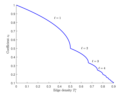
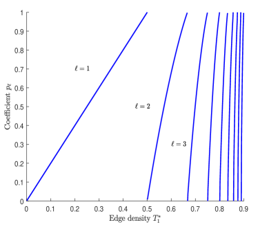
Figure 3: $c_{\ell}$ (left) and $p_{\ell}$ (right) as a function of $T_{1}^{*}$.

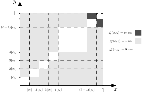
Figure 4: $g_{\ell}^{*}$ for $\ell\in\mathbb{N}$ and $T_{1}^{*}\in(\frac{\ell-1}{\ell},\frac{\ell}{\ell+1}]$.

3 Main results

In Section 3.1 we state two assumptions. In Section 3.2 we identify the scaling behaviour of $s_{\infty}$ for fixed $T_{1}^{*}$ and $T_{2}^{*}\downarrow T_{1}^{*3}$, respectively, $T_{2}^{*}\uparrow T_{1}^{*3}$. It turns out that the way in which $s_{\infty}$ tends to zero differs in these two cases. In Section 3.3 we characterise the asymptotic structure of random graphs drawn from the microcanonical ensemble for fixed $T_{1}^{*}$ and $T_{2}^{*}\downarrow T_{1}^{*3}$, respectively, $T_{2}^{*}\uparrow T_{1}^{*3}$. It turns out that the structure differs in these two cases.

3.1 Assumptions

Throughout the sequel we make the following two assumptions:

Assumption 1

Fix the edge density $T_{1}^{*}\in(0,1)$ and consider the triangle density $T_{1}^{*3}+\epsilon$ for some $\epsilon$, either positive or negative. Consider the associated Lagrange multipliers $\vec{\theta}^{*}_{\infty}(\epsilon):=(\theta^{*}_{1}(\epsilon),\theta^{*}_{2}(\epsilon))$. Then, for $\epsilon$ sufficiently small, we have the representation

$$\sup_{\tilde{h}\in\tilde{W}}\left[\theta_{1}^{*}(\epsilon)T_{1}(\tilde{h})+\theta_{2}^{*}(\epsilon)T_{2}(\tilde{h})-I(\tilde{h})\right]=[\theta_{1}T_{1}^{*}-I(T_{1}^{*})]+(\gamma_{1}T_{1}^{*}+\gamma_{2}T_{1}^{*3})\epsilon+O(\epsilon^{2}),$$ (3.1)

where $\theta_{1}:=\theta^{*}_{1}(0),\gamma_{1}=\theta^{*^{\prime}}_{1}(0)$ and $\gamma_{2}=\theta^{*^{\prime}}_{2}(0)$. (It turns out that $\theta_{2}:=\theta^{*}_{2}(0)=0$.)

Assumption 2

Fix the edge density $T_{1}^{*}\in(0,1)$ and consider the triangle density $T_{1}^{*3}+\epsilon$ for some $\epsilon$, either positive or negative. Consider the microcanonical entropy

$$-J(\epsilon):=\sup\{-I(\tilde{h}):~{}\tilde{h}\in\tilde{W},~{}T_{1}(\tilde{h})=T_{1}^{*},~{}T_{2}(\tilde{h})=T_{1}^{*3}+\epsilon\}.$$ (3.2)

Then, for $\epsilon$ sufficiently small, the maximizer $h_{\epsilon}^{*}$ of (3.2) has the form

$$h_{\epsilon}^{*}=T_{1}^{*}+g_{\epsilon},\qquad g_{\epsilon}=g_{11}1_{I\times I}+g_{12}1_{(I\times J)\cup(J\times I)}+g_{22}1_{J\times J},$$ (3.3)

for some $g_{11},g_{12},g_{22}\in[-T_{1}^{*},1-T_{1}^{*}]$ and $I,J\subset[0,1]$.

Remark 3.1

Assumption 1 is needed to prove Theorems 3.3–3.5. In Section 4.1 we show that Assumption 1 is true when $T_{1}^{*}\in[\frac{1}{2},1)$, which implies the scalings in (3.4) and (3.6) below. We can prove the scalings in (3.4) and (3.5) below without Assumption 1, but at the cost of replacing ‘$=$’ by ‘$\geq$’ and replacing $\lim$ by $\limsup$. If Assumption 1 fails, then these scalings hold with strict inequality.

Remark 3.2

Assumption 2 is needed to prove Propositions 3.7–3.8. Importantly, the validity of Assumption 2 is firmly backed by the extensive numerical experiments performed in [21], showing that close to the ER line the optimizing graphon has the form (3.3). The assumption reflects the following informal argument. Suppose that we want to maximise the microcanonical entropy among block graphons. Then we expect the entropy to decrease when we add more structure to the graphon. An $m\times m$ block graphon corresponds to a random graph where the vertices are divided into $m$ groups, and within each group we have an Erdős-Rényi random graph with a certain retention probability. We expect that the microcanonical entropy decreases as $m$ increases.

3.2 Scaling of the specific relative entropy

The variational problem $J(\epsilon)$ in (3.2) was solved in [22] for the case $\epsilon>0$, while the case $\epsilon$ remained unsolved. We consider small $\epsilon$ only, which is simpler and yields more intuition about the way the constraint is achieved. In [20] the maximisers of the microcanonical entropy are identified numerically. The optimal graphons obtained agree with the optimal graphons that we derive rigorously.

Theorem 3.3

For $T_{1}^{*}\in(0,1)$ and $T_{1}^{*}\neq\frac{1}{2}$,

$$\lim_{\epsilon\downarrow 0}\,\epsilon^{-1}s_{\infty}(T_{1}^{*},T_{1}^{*3}+3T_{1}^{*}\epsilon)=A(T_{1}^{*}):=-\frac{1}{1-2T_{1}^{*}}\log\frac{T_{1}^{*}}{1-T_{1}^{*}}\in(0,\infty).$$ (3.4)

Theorem 3.4

For $T_{1}^{*}\in(0,\frac{1}{2}]$,

$$\lim_{\epsilon\downarrow 0}\,\epsilon^{-2/3}s_{\infty}(T_{1}^{*},T_{1}^{*3}-T_{1}^{*3}\epsilon)=B(T^{*}_{1}):=\frac{1}{4}\frac{T_{1}^{*}}{1-T_{1}^{*}}\in(0,\infty).$$ (3.5)

Theorem 3.5

For $T_{1}^{*}\in(\frac{1}{2},1)$,

$$\lim_{\epsilon\downarrow 0}\epsilon^{-2/3}s_{\infty}(T_{1}^{*},T_{1}^{*3}-T_{1}^{*3}\epsilon)=f(T_{1}^{*},y^{*})\in(0,\infty),$$ (3.6)

where $y^{*}=y^{*}(T^{*}_{1})\in(-T_{1}^{*},0)$ is the unique point where the function $x\mapsto f(T_{1}^{*},x)$ defined by

$$f(T_{1}^{*},x):=T_{1}^{*2}\frac{I(T_{1}^{*}+x)-I(T_{1}^{*})-I^{\prime}(T_{1}^{*})x}{x^{2}},\quad x\in(-T^{*}_{1},0),$$ (3.7)

attains its global minimum.

The main implication of Theorems 3.3–3.5 is that, for a fixed value of the edge density, it is less costly in terms of relative entropy to increase the density of triangles than to decrease the density of triangles. Above the ER line the cost is linear in the distance, below the ER line the cost is proportional to the $\tfrac{2}{3}$-power of the distance.

For the case $T_{1}^{*}\in[\frac{1}{2},1)$ the above results are illustrated in Figure 5. In the left panel we plot $\epsilon^{2/3}f(T_{1}^{*},y^{*})$, in the right panel we plot $\epsilon A(T^{*}_{1})$. In both panels we take $\epsilon$ sufficiently small and pick four different values of $T_{1}^{*}$.

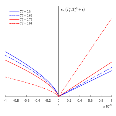
Figure 5: Limit of scaled $s_{\infty}$ as a function of $\epsilon$ for $\epsilon$ sufficiently small.

3.3 Scaling of the optimal graphon

In Propositions 3.6–3.8 below we identify the structure of the optimal graphons corresponding to the perturbed constraints in the microcanonical ensemble in the limit as $n\to\infty$.

Proposition 3.6

For the pair of constraints $(T_{1}^{*},T_{1}^{*3}+3T_{1}^{*}\epsilon)$ with $\epsilon>0$ sufficiently small, the unique optimiser $h_{\epsilon}^{*}$ of the microcanonical entropy is given by

$$h_{\epsilon}^{*}(x,y)=\left\{\begin{array}[]{ll}\hskip 2.0pth_{11}+o(\epsilon),&(x,y)\in[0,\lambda\epsilon]^{2},\\[5.69046pt] 1-T_{1}^{*}+h_{1}\epsilon+o(\epsilon),&(x,y)\in[0,\lambda\epsilon]\times(\lambda\epsilon,1]\cup(\lambda\epsilon,1]\times[0,\lambda\epsilon],\\[5.69046pt] T_{1}^{*}+h_{2}\epsilon+o(\epsilon),&(x,y)\in(\lambda\epsilon,1]^{2},\\ \end{array}\right.$$ (3.8)

where

$$\lambda:=\frac{1}{(1-2T_{1}^{*})^{2}},\qquad h_{1}:=\frac{1}{2}h_{2},\qquad\qquad h_{2}:=-\frac{2}{1-2T_{1}^{*}},$$ (3.9)

and $h_{11}$ solves the equation $I^{\prime}(h_{11})=3I^{\prime}(1-T_{1}^{*})$.

Proposition 3.7

For $T_{1}^{*}\in(0,\frac{1}{2}]$ and $T_{2}^{*}=T_{1}^{*3}-3T_{1}^{*}\epsilon$, $\epsilon\downarrow 0$, the optimal graphon is given by

$$h^{*}_{\epsilon}=T_{1}^{*}+\epsilon^{1/3}{g}^{*}+o(\epsilon^{2/3})\qquad\text{\em(global perturbation)}$$ (3.10)

with $g^{*}$ defined by

$$g^{*}(x,y)=\left\{\begin{array}[]{ll}-T_{1}^{*},&(x,y)\in[0,\frac{1}{2}]^{2},\\[5.69046pt] \hskip 5.0ptT_{1}^{*},&(x,y)\in[0,\frac{1}{2}]\times(\frac{1}{2},1]\cup(\frac{1}{2},1]\times[0,\frac{1}{2}],\\[5.69046pt] -T_{1}^{*},&(x,y)\in(\frac{1}{2},1]^{2}.\\ \end{array}\right.$$ (3.11)

Proposition 3.8

For $T_{1}^{*}\in(\frac{1}{2},1)$ and $T_{2}^{*}=T_{1}^{*3}-3T_{1}^{*}\epsilon$, $\epsilon\downarrow 0$, the optimal graphon is given by

$$h^{*}_{\epsilon}=T_{1}^{*}+g_{\epsilon}^{*}\qquad\text{\em(local perturbation)}$$ (3.12)

with $g_{\epsilon}^{*}$ defined by

$$g_{\epsilon}^{*}(x,y):=\begin{cases}~{}\frac{T_{1}^{*2}}{y*}\epsilon^{2/3},~{}&\qquad(x,y)\in[0,1-\frac{T_{1}^{*}}{|y^{*}|}\epsilon^{1/3}]^{2},\\[5.69046pt] ~{}T_{1}^{*}\epsilon^{1/3},~{}&\qquad(x,y)\in[0,1-\frac{T_{1}^{*}}{|y^{*}|}\epsilon^{1/3}]\times[1-\frac{T_{1}^{*}}{|y^{*}|}\epsilon^{1/3},1],\\[5.69046pt] &\qquad\text{ {\rm or} }(x,y)\in[1-\frac{T_{1}^{*}}{|y^{*}|}\epsilon^{1/3},1]\times[0,1-\frac{T_{1}^{*}}{|y^{*}|}\epsilon^{1/3}],\\[5.69046pt] ~{}y^{*},~{}&\qquad(x,y)\in[1-\frac{T_{1}^{*}}{|y^{*}|}\epsilon^{1/3},1]^{2},\end{cases}$$ (3.13)

where $y^{*}\in(-T_{1}^{*},0)$ is as in Theorem 3.5.

The main implication of Propositions 3.6–3.8 is that the optimal perturbation of the Erdős-Rényi graphon is global above the ER line and also below the ER line when the edge density is less than or equal to $\tfrac{1}{2}$, whereas it is local below the ER line when the edge density is larger than $\tfrac{1}{2}$.

4 Proofs of Theorems 3.3–3.5

In Sections 4.1–4.3 we prove Theorems 3.3–3.5, respectively. Along the way we use Propositions 3.6–3.8, which we prove in Section 5.

4.1 Proof of Theorem 3.3

Let

$$T_{1}(\epsilon)=T_{1}^{*},\qquad T_{2}(\epsilon)=T_{1}^{*3}+3T_{1}^{*3}\epsilon.$$ (4.1)

The factor $3T_{1}^{*}$ appearing in front of the $\epsilon$ is put in for convenience. We know that for every pair of graphical constraints $(T_{1}(\epsilon),T_{2}(\epsilon))$ there exists a unique pair of Lagrange multipliers $(\theta_{1}(\epsilon),\theta_{2}(\epsilon))$ corresponding to these constraints (to ease the notation we suppress $*$). For an elaborate discussion on existence and uniqueness we refer the reader to [18]. By considering the Taylor expansion of the Lagrange multipliers $(\theta_{1}(\epsilon),\theta_{2}(\epsilon))$ around $\epsilon=0$, we obtain

$$\theta_{1}(\epsilon)=\theta_{1}+\gamma_{1}\epsilon+\tfrac{1}{2}\Gamma_{1}\epsilon^{2}+O(\epsilon^{3}),\qquad\theta_{2}(\epsilon)=\gamma_{2}\epsilon+\tfrac{1}{2}\Gamma_{2}\epsilon^{2}+O(\epsilon^{3}),$$ (4.2)

where

$$\theta_{1}(0)=\theta_{1}=I^{\prime}(T_{1}^{*}),\>~{}\gamma_{1}=\theta^{\prime}_{1}(0),\>~{}\Gamma_{1}=\theta^{\prime\prime}_{1}(0),\>~{}\theta_{2}(0)=0,\>~{}\gamma_{2}=\theta^{\prime}_{2}(0),\>~{}\Gamma_{2}=\theta^{\prime\prime}_{2}(0).$$ (4.3)

These equalities follow from [18, Lemma 5.3]. For $\epsilon=0$ we have $T_{2}^{*}(0)=T_{1}^{*3}$, which shows that the constraints correspond to those of the Erdős-Rényi random graph. We denote the two terms in the expression for $s_{\infty}$ in (2.32) by $I_{1},I_{2}$, i.e., $s_{\infty}=I_{1}-I_{2}$ with

$$I_{1}:=\sup_{\tilde{h}\in\tilde{W}}\big{[}\vec{\theta}_{\infty}\cdot\vec{T}(\tilde{h})-I(\tilde{h})\big{]},\>\>\>I_{2}:=\sup_{\tilde{h}\in\tilde{W}^{*}}\big{[}\vec{\theta}_{\infty}\cdot\vec{T}(\tilde{h})-I(\tilde{h})\big{]},$$ (4.4)

and let $s_{\infty}(\epsilon)$ denote the relative entropy corresponding to the perturbed constraints. We distinguish between the cases $T_{1}^{*}\in[\frac{1}{2},1)$ and $T_{1}^{*}\in(0,\frac{1}{2})$.

Case I $T_{1}^{*}\in[\frac{1}{2},1)$:

According to [18, Section 5], if $T_{1}^{*}\in[\frac{1}{2},1)$ and $T_{2}^{*}\in[\frac{1}{8},1)$, then the corresponding Lagrange multipliers $(\theta_{1},\theta_{2})$ are both non-negative. Hence by [8, Theorem 4.1] we have that

$$I_{1}:=\sup_{\tilde{h}\in\tilde{W}}\left[\theta_{1}(\epsilon)T_{1}(\tilde{h})+\theta_{2}(\epsilon)T_{2}(\tilde{h})-I(\tilde{h})\right]=\sup_{0\leq u\leq 1}\left[\theta_{1}(\epsilon)u+\theta_{2}(\epsilon)u^{3}-I(u)\right],$$ (4.5)

and, consequently,

$$I_{1}=\theta_{1}(\epsilon)u^{*}(\epsilon)+\theta_{2}(\epsilon)u^{*}(\epsilon)^{3}-I(u^{*}(\epsilon)).$$ (4.6)

The optimiser $u^{*}(\epsilon)\in(0,1)$ corresponding to the perturbed multipliers $\theta_{1}(\epsilon)$ and $\theta_{2}(\epsilon)$ is analytic in $\epsilon$, as shown in [30]. Therefore, a Taylor expansion around $\epsilon=0$ gives

$$u^{*}(\epsilon)=T_{1}^{*}+\delta\epsilon+\tfrac{1}{2}\Delta\epsilon^{2}+O(\epsilon^{3}),$$ (4.7)

where $\delta={u^{*}}^{\prime}(0)$ and $\Delta={u^{*}}^{\prime\prime}(0)$. Hence $I_{1}$ can be written as

$$I_{1}=\theta_{1}T_{1}^{*}-I(T_{1}^{*})+(\gamma_{1}T_{1}^{*}+\gamma_{2}T_{1}^{*3})\epsilon+O(\epsilon^{2}).$$ (4.8)

Moreover,

$$I_{2} =\big{[}\theta_{1}+\gamma_{1}\epsilon+\tfrac{1}{2}\Gamma_{1}\epsilon^{2}+O(\epsilon^{3})\big{]}T_{1}^{*}+\big{[}\gamma_{2}\epsilon+\tfrac{1}{2}\Gamma_{2}\epsilon^{2}+O(\epsilon^{3})\big{]}(T_{1}^{*3}+3T_{1}^{*}\epsilon)-\inf_{\tilde{h}\in\tilde{W}_{\epsilon}^{*}}I(\tilde{h})$$ (4.9)

$$=\theta_{1}T_{1}^{*}+\gamma_{1}T_{1}^{*}\epsilon+\tfrac{1}{2}\Gamma_{1}T_{1}^{*}\epsilon^{2}+T_{1}^{*3}\gamma_{2}\epsilon+\tfrac{1}{2}\Gamma_{2}T_{1}^{*3}\epsilon^{2}+3T_{1}^{*}\gamma_{2}\epsilon^{2}-J^{\downarrow}(\epsilon)+O(\epsilon^{3}),$$

where

$$J^{\downarrow}(\epsilon):=\inf_{\tilde{h}\in\tilde{W}_{\epsilon}^{*}}I(\tilde{h}),\qquad\tilde{W}_{\epsilon}^{*}:=\{\tilde{h}\in\tilde{W}\colon\,T_{1}(\tilde{h})=T_{1}^{*},\ T_{2}(\tilde{h})=T_{1}^{*3}+3T_{1}^{*}\epsilon\}.$$ (4.10)

Consequently,

$$s_{\infty}(T_{1}^{*},T_{1}^{*3}+3T_{1}^{*3}\epsilon)=J^{\downarrow}(\epsilon)-I(T_{1}^{*})+O(\epsilon^{2}).$$ (4.11)

A straightforward computation of the entropy of $h_{\epsilon}^{*}$ in (3.8) shows that

$$J^{\downarrow}(\epsilon)=I(T_{1}^{*})+I^{\prime}(T_{1}^{*})h_{2}\epsilon+o(\epsilon)=I(T_{1}^{*})-\frac{1}{1-2T_{1}^{*}}\log\frac{T_{1}^{*}}{1-T_{1}^{*}}\epsilon+o(\epsilon).$$ (4.12)

Hence we obtain that

$$s_{\infty}(T_{1}^{*},T_{1}^{*3}+3T_{1}^{*3}\epsilon)=-\frac{1}{1-2T_{1}^{*}}\log\frac{T_{1}^{*}}{1-T_{1}^{*}}\,\epsilon+o(\epsilon).$$ (4.13)

Case II $T_{1}^{*}\in(0,\frac{1}{2})$:

Consider the term

$$I_{1}:=\sup_{\tilde{h}\in\tilde{W}}\left[\theta_{1}(\epsilon)T_{1}(\tilde{h})+\theta_{2}(\epsilon)T_{2}(\tilde{h})-I(\tilde{h})\right],$$ (4.14)

as above. If Assumption 1 applies, then this case can be treated in the same way as Case I. Otherwise, consider the lower bound

$$\sup_{\tilde{h}\in\tilde{W}}\left[\theta_{1}(\epsilon)T_{1}(\tilde{h})+\theta_{2}(\epsilon)T_{2}(\tilde{h})-I(\tilde{h})\right]\geq\sup_{0\leq u\leq 1}\left[\theta_{1}(\epsilon)u+\theta_{2}(\epsilon)u^{3}-I(u)\right].$$ (4.15)

The arguments for Case I following (4.6) still apply, and (4.11) is obtained with an inequality instead of an equality.

4.2 Proof of Theorem 3.4

In this section we omit the computations that are similar to those in the proof of Theorem 3.3, as provided in Section 4.1. Let

$$T_{1}(\epsilon)=T_{1}^{*},\qquad T_{2}(\epsilon)=T_{1}^{*3}-T_{1}^{*3}\epsilon.$$ (4.16)

The factor $T_{1}^{*3}$ appearing in front of $\epsilon$ is put in for convenience (without loss of generality). The perturbed Lagrange multipliers are

$$\theta_{1}(\epsilon)=\theta_{1}+\gamma_{1}\epsilon+\tfrac{1}{2}\Gamma_{1}\epsilon^{2}+O(\epsilon^{3}),\qquad\theta_{2}(\epsilon)=\gamma_{2}\epsilon+\tfrac{1}{2}\Gamma_{2}\epsilon^{2}+O(\epsilon^{3}),$$ (4.17)

where

$$\theta_{1}=I^{\prime}(T_{1}^{*}),\qquad\gamma_{1}=\theta^{\prime}_{1}(0),\qquad\Gamma_{1}=\theta^{\prime\prime}_{1}(0)\qquad\gamma_{2}=\theta^{\prime}_{2}(0),\qquad\Gamma_{2}=\theta^{\prime\prime}_{2}(0).$$ (4.18)

We denote the two terms in the expression for $s_{\infty}$ in (2.32) by $I_{1},I_{2}$, i.e., $s_{\infty}=I_{1}-I_{2}$, and let $s_{\infty}(\epsilon)$ denote the perturbed relative entropy. The computations for $I_{1}$ are similar as before, because the exact form of the constraint does not affect the expansions in (4.7) and (4.8). For $I_{2}$, on the other hand, we have

$$I_{2} =\theta_{1}T_{1}^{*}+\gamma_{1}T_{1}^{*}\epsilon+\tfrac{1}{2}\Gamma_{1}T_{1}^{*}\epsilon^{2}+T_{1}^{*3}\gamma_{2}\epsilon+\tfrac{1}{2}\Gamma_{2}T_{1}^{*3}\epsilon^{2}-T_{1}^{*3}\gamma_{2}\epsilon^{2}-J_{1}^{\uparrow}(\epsilon)+\,O(\epsilon^{3})$$ (4.19)

$$=\theta_{1}T_{1}^{*}+\gamma_{1}T_{1}^{*}\epsilon+T_{1}^{*3}\gamma_{2}\epsilon-J_{1}^{\uparrow}(\epsilon)+O(\epsilon^{2}),$$

where

$$J_{1}^{\uparrow}(\epsilon):=\inf_{\tilde{h}\in\tilde{W}_{\epsilon}^{*}}I(\tilde{h}),\qquad\tilde{W}_{\epsilon}^{*}:=\big{\{}\tilde{h}\in\tilde{W}\colon\,T_{1}(\tilde{h})=T_{1}^{*},\ T_{2}(\tilde{h})=T_{1}^{*3}-T_{1}^{*3}~{}\epsilon\big{\}}.$$ (4.20)

Consequently,

$$s_{\infty}(T_{1}^{*},T_{1}^{*}-T_{1}^{*3}\epsilon)=J_{1}^{\uparrow}(\epsilon)-I(T_{1}^{*})+O(\epsilon^{2}).$$ (4.21)

Denote by $\tilde{h}_{\epsilon}^{*}$ the optimiser of the variational problem $J_{1}^{\uparrow}(\epsilon)$, as defined in (4.20). From Proposition 3.7 we know that, for $T_{1}^{*}\in(0,\frac{1}{2}]$, any optimal graphon in the equivalence class $\tilde{h}_{\epsilon}^{*}$, denoted by $h_{\epsilon}^{*}$ for simplicity in the notation, has the form

$$h_{\epsilon}^{*}=T_{1}^{*}+\epsilon^{1/3}{g}^{*}+o(\epsilon^{2/3})$$ (4.22)

with $g^{*}$ given by

$$g^{*}(x,y)=\left\{\begin{array}[]{ll}-T_{1}^{*},&(x,y)\in[0,\frac{1}{2}]^{2},\\[5.69046pt] \hskip 5.0ptT_{1}^{*},&(x,y)\in[0,\frac{1}{2}]\times(\frac{1}{2},1]\cup(\frac{1}{2},1]\times[0,\frac{1}{2}],\\[5.69046pt] -T_{1}^{*},&(x,y)\in(\frac{1}{2},1]^{2}.\\ \end{array}\right.$$ (4.23)

Hence

$$J_{1}^{\uparrow}(\epsilon)=I(T_{1}^{*})+\frac{1}{2}T_{1}^{*2}I^{\prime\prime}(T_{1}^{*})\epsilon^{2/3}+o(\epsilon^{2/3})=I(T_{1}^{*})+\frac{1}{4}\frac{T_{1}^{*}}{1-T_{1}^{*}}\epsilon^{2/3}+o(\epsilon^{2/3}),$$ (4.24)

which gives

$$s_{\infty}(T_{1}^{*},T_{1}^{*}-T_{1}^{*3}\epsilon)=\frac{1}{4}\frac{T_{1}^{*}}{1-T_{1}^{*}}\epsilon^{2/3}+o(\epsilon^{2/3}).$$ (4.25)

4.3 Proof of Theorem 3.5

The computations leading to the expression for the relative entropy in the right-hand side of (3.6) are similar to those in Section 4.2, and we omit them. Hence we have

$$s_{\infty}(T_{1}^{*},T_{1}^{*}-T_{1}^{*3}\epsilon)=J_{2}^{\uparrow}(\epsilon)-I(T_{1}^{*})+O(\epsilon^{2}),$$ (4.26)

where, for $T_{1}^{*}\in(\frac{1}{2},1)$,

$$J_{2}^{\uparrow}(\epsilon):=\inf_{\tilde{h}\in\tilde{W}_{\epsilon}^{*}}I(\tilde{h}),\qquad\tilde{W}_{\epsilon}^{*}:=\big{\{}\tilde{h}\in\tilde{W}:T_{1}(\tilde{h})=T_{1}^{*},\ T_{2}(\tilde{h})=T_{1}^{*3}-T_{1}^{*3}~{}\epsilon\big{\}}.$$ (4.27)

Denote by $\tilde{h}_{\epsilon}^{*}$ the optimiser of the variational problem $J_{2}^{\uparrow}(\epsilon)$, as defined in (4.27). From Proposition 3.8 we know that, for $T_{1}^{*}\in(\frac{1}{2},1)$, any optimal graphon in the equivalence class $\tilde{h}_{\epsilon}^{*}$, denoted by $h_{\epsilon}^{*}$ for simplicity in the notation, has the form

$$h_{\epsilon}^{*}=T_{1}^{*}+g_{\epsilon}^{*}$$ (4.28)

with $g_{\epsilon}^{*}$ given by

$$g_{\epsilon}^{*}(x,y):=\begin{cases}~{}{\displaystyle\tfrac{T_{1}^{*2}}{y^{*}}}\epsilon^{2/3},~{}&\qquad(x,y)\in[0,1-{\displaystyle\tfrac{T_{1}^{*}}{|y^{*}|}}\epsilon^{1/3}]\times[0,1-{\displaystyle\tfrac{T_{1}^{*}}{|y^{*}|}}\epsilon^{1/3}],\\ \vspace{-4mm}&\\ ~{}T_{1}^{*}\epsilon^{1/3},~{}&\qquad(x,y)\in[0,1-{\displaystyle\tfrac{T_{1}^{*}}{|y^{*}|}}\epsilon^{1/3}]\times[1-{\displaystyle\tfrac{T_{1}^{*}}{|y^{*}|}}\epsilon^{1/3},1]\\ \vspace{-4mm}&\\ &\qquad~{}\text{ {\rm or} }(x,y)\in[1-{\displaystyle\tfrac{T_{1}^{*}}{|y^{*}|}}\epsilon^{1/3},1]\times[0,1-{\displaystyle\tfrac{T_{1}^{*}}{|y^{*}|}}\epsilon^{1/3}],\\ \vspace{-4mm}&\\ ~{}y^{*},~{}&\qquad(x,y)\in[1-{\displaystyle\tfrac{T_{1}^{*}}{|y^{*}|}}\epsilon^{1/3},1]\times[1-{\displaystyle\tfrac{T_{1}^{*}}{|y^{*}|}}\epsilon^{1/3},1].\end{cases}$$ (4.29)

Hence we have

$$s_{\infty}(T_{1}^{*},T_{1}^{*}-T_{1}^{*3}\epsilon)=f(T_{1}^{*},y^{*})\epsilon^{2/3}+o(\epsilon^{2/3}),$$ (4.30)

where $y^{*}\in(-T_{1}^{*},0)$ minimizes the function $x\mapsto f(T_{1}^{*},x)$ defined by

$$f(T_{1}^{*},x):=T_{1}^{*2}\frac{I(T_{1}^{*}+x)-I(T_{1}^{*})-I^{\prime}(T_{1}^{*})x}{x^{2}},\quad x\in(-T_{1}^{*},0).$$ (4.31)

We proceed by showing that $x\mapsto f(T_{1}^{*},x)$ has a unique minimizer $y^{*}\in(-T_{1}^{*},0).$

$\circ$ First, we show that $f(T_{1}^{*},x)>0$ for every $T_{1}^{*}\in(0,1)$ and every $x\in(-T_{1}^{*},0)$, or equivalently

$$I(T_{1}^{*}+x)-I(T_{1}^{*})-I^{\prime}(T_{1}^{*})x>0.$$ (4.32)

From the mean-value theorem we have that, for any given $x\in(-T_{1}^{*},0)$, there exists $\xi\in(T_{1}^{*}+x,T_{1}^{*})$ such that $I^{\prime}(T_{1}^{*}+x)-I(T_{1}^{*})=I^{\prime}(\xi)x$. Because $I^{\prime}$ is an increasing function, this implies that

$$f(T_{1}^{*},x)=(I^{\prime}(\xi)-I^{\prime}(T_{1}^{*}))x>0,$$ (4.33)

recalling that $x\in(-T_{1}^{*},0)$ and $\xi\in(T_{1}^{*}+x,T_{1}^{*})$.

$\circ$ Second, we show that the function $x\mapsto f(T_{1}^{*},x)$ attains a unique minimum at some point $y^{*}\in(-T_{1}^{*},0)$. A straightforward computation shows that the derivative of $f(T_{1}^{*},\cdot)$ is equal to

$$f^{\prime}(T_{1}^{*},x)=T_{1}^{*2}\frac{\left(I^{\prime}(T_{1}^{*}+x)-I^{\prime}(T_{1}^{*})\right)x^{2}-2x\left(I(T_{1}^{*}+x)-I(T_{1}^{*})-I^{\prime}(T_{1}^{*})x\right)}{x^{4}}.$$ (4.34)

Substituting $x=0$ we observe that $f^{\prime}(T_{1}^{*},0)=\frac{1}{6}(T_{1}^{*})^{2}\,I^{(4)}(T_{1}^{*})>0$, and by taking the limit $x\rightarrow-T_{1}^{*}$ we observe that

$$\lim_{x\rightarrow-T_{1}^{*}}f^{\prime}(T_{1}^{*},x)=-\infty.$$ (4.35)

Hence the function $f(T_{1}^{*},\cdot)$ is decreasing in a neighborhood of $-T_{1}^{*}$, while it is increasing in a neighborhood of zero. Consequently, there must be at least one point in $(-T_{1}^{*},0)$ where the derivative is zero.

$\circ$ It remains to show that there is a unique point $y^{*}$ in $(-T_{1}^{*},0)$ where the derivative is zero. Suppose that $y^{*}$ is such a point where $f^{\prime}(T_{1}^{*},y^{*})=0$. Then from (4.34) we know that

$$\left(I^{\prime}(T_{1}^{*}+y^{*})-I^{\prime}(T_{1}^{*})\right)y^{*}-2\left(I(T_{1}^{*}+y^{*})-I(T_{1}^{*})-I^{\prime}(T_{1}^{*})y^{*}\right)=0.$$ (4.36)

From the mean-value theorem we know that there exist $\xi_{1}\in(T_{1}^{*}+y^{*},T_{1}^{*})$ and $\xi_{2}\in(T_{1}^{*}+y^{*},T_{1}^{*})$ such that $I^{\prime\prime}(\xi_{1})y^{*}=I^{\prime}(T_{1}^{*}+y^{*})-I^{\prime}(T_{1}^{*})$ and $I^{\prime}(\xi_{2})y^{*}=I(T_{1}^{*}+y^{*})-I(T_{1}^{*})$. Moreover, $\xi_{2}$ is unique since $I$ is a convex function. This is not necessarily true for $\xi_{1}$. Hence (4.36) becomes

$$I^{\prime\prime}(\xi_{1})y^{*}-2(I^{\prime}(\xi_{2})-I^{\prime}(T_{1}^{*}))=0.$$ (4.37)

Applying again the mean-value theorem, we get that there exists a, not necessarily unique, $\xi_{3}\in(\xi_{2},T_{1}^{*})$ such that $I^{\prime}(\xi_{2})-I^{\prime}(T_{1}^{*})=I^{\prime\prime}(\xi_{3})(\xi_{2}-T_{1}^{*})$. Substituting this into (4.37), we obtain

$$I^{\prime\prime}(\xi_{1})y^{*}-2I^{\prime\prime}(\xi_{3})(\xi_{2}-T_{1}^{*})=0.$$ (4.38)

Hence any possible solution $y^{*}$ satisfies the equation

$$y^{*}=-\frac{2I^{\prime\prime}(\xi_{3})(T_{1}^{*}-\xi_{2})}{I^{\prime\prime}(\xi_{1})}=-\frac{2\xi_{1}(1-\xi_{1})(T_{1}^{*}-\xi_{2})}{\xi_{3}(1-\xi_{3})}.$$ (4.39)

Multiple solutions may arise due to the non-uniqueness of $\xi_{1}$ and $\xi_{3}$. Notice that if the function $I^{\prime}$ attains a given slope at some $\xi^{*}$, it does so as well at $1-\xi^{*}$ (and nowhere else); use that $I^{\prime\prime}(u)$ is given by $1/(u(1-u))$. Therefore, other possible solutions may occur when we replace $\xi_{1}$ by $1-\xi_{1}$ and/or $\xi_{3}$ by $1-\xi_{3}$. However, it is directly seen that the right-hand side of (4.39) is invariant under this substitution. Hence the point $y^{*}$ where the derivative of $f(T_{1}^{*},\cdot)$ is equal to zero is unique. We finalize the proof of Proposition 3.8 in the next section.

5 Proofs of Propositions 3.6–3.8

In Section 5.1 we state two lemmas (Lemmas 5.1–5.2 below) about variational formulas encountered in Section 4, and use them to prove Propositions 3.6–3.8. In Section 5.2 we provide the proof of these two lemmas, which requires an additional lemma about a certain function related to (4.31) (Lemma 5.3 below), whose proof is deferred to Section 5.3.

5.1 Key lemmas

In Section 4 the following variational problems were encountered:

• For $T_{1}^{*}\in(0,1)$,

  $$J^{\downarrow}(\epsilon)=\inf\big{\{}I(\tilde{h})\colon\,\tilde{h}\in\tilde{W},\,T_{1}(\tilde{h})=T_{1}^{*},\,T_{2}(\tilde{h})=T_{1}^{*3}+3T_{1}^{*3}\epsilon\big{\}}.$$ (5.1)

• For $T_{1}^{*}\in(0,\frac{1}{2}]$,

  $$J_{1}^{\uparrow}(\epsilon)=\inf\big{\{}I(\tilde{h})\colon\,\tilde{h}\in\tilde{W},\,T_{1}(\tilde{h})=T_{1}^{*},\,T_{2}(\tilde{h})=T_{1}^{*3}-T_{1}^{*3}\epsilon\big{\}}.$$ (5.2)

• For $T_{1}^{*}\in(\frac{1}{2},1)$,

  $$J_{2}^{\uparrow}(\epsilon)=\inf\big{\{}I(\tilde{h})\colon\,\tilde{h}\in\tilde{W},\,T_{1}(\tilde{h})=T_{1}^{*},\,T_{2}(\tilde{h})=T_{1}^{*3}-T_{1}^{*3}\epsilon\big{\}}.$$ (5.3)

The difference between the variational problems in (5.2) and (5.3) lies only in the possible values $T_{1}^{*}$ can take. We give them separate displays in order to easily refer to them later on.

In order to prove Propositions 3.6–3.8, we need to analyse the above three variational problems for $\epsilon$ sufficiently small. The variational formula in (5.1) was already analysed in [22]. Solving the equations given in [22, Theorem 1.1] for the case of triangle density equal to $T_{1}^{*3}+3T_{1}^{*3}\epsilon$ and $\epsilon$ sufficiently small enough we obtain the graphon given in (3.8). In what follows we concentrate on the variational formulas in (5.2) and (5.3). We analyse the latter with the help of a perturbation argument. In particular, we show that the optimal perturbations are those given in (3.10) and (3.12), respectively. The claims in Propositions 3.7 and 3.8 follow directly from the following two lemmas.

We remind the reader that Assumption 2 is in forse, i.e., we look for the optimal graphon in the class of two-step graphons.

Lemma 5.1

Let $T_{1}^{*}\in(0,\frac{1}{2}]$. For $\epsilon>0$ sufficiently small,

$$J_{1}^{\uparrow}(\epsilon)=I(T_{1}^{*})+\frac{1}{4}\frac{T_{1}^{*}}{1-T_{1}^{*}}\epsilon^{2/3}+o(\epsilon^{2/3}).$$ (5.4)

Lemma 5.2

Let $T_{1}^{*}\in(\frac{1}{2},1)$. For $\epsilon>0$ sufficiently small,

$$J_{2}^{\uparrow}(\epsilon)=I(T_{1}^{*})+f(T_{1}^{*},y^{*})\epsilon^{2/3}+o(\epsilon^{2/3}),$$ (5.5)

where $f(T_{1}^{*},x)$, $x\in(-T_{1}^{*},0)$, and $y^{*}$ are as defined in Theorem 3.5.

In what follows we use the notation $f(\epsilon)\asymp g(\epsilon)$ when ${f(\epsilon)}/{g(\epsilon)}$ converges to a positive finite constant as $\epsilon\downarrow 0$, and $f(\epsilon)=\omega(g(\epsilon))$ when ${f(\epsilon)}/{g(\epsilon)}$ diverges as $\epsilon\downarrow 0$.

5.2 Proof of Lemmas 5.1–5.2

Proof.   Instead of the variational problems ${J}_{1}^{\uparrow}(\epsilon)$ and ${J}_{2}^{\uparrow}(\epsilon)$ we will consider for $\epsilon>0$ the variational problem

$${J}^{\uparrow}(\epsilon)=\inf\{I(\tilde{h}):\tilde{h}\in\tilde{W},T_{1}(\tilde{h})=T_{1}^{*},T_{2}(\tilde{h})=T_{1}^{*3}-T_{1}^{*3}\epsilon\}.$$ (5.6)

Below we provide the technical details leading to the optimal perturbation corresponding to (5.6). At some point we will distinguish between the two cases $T_{1}^{*}\in(0,\frac{1}{2})$ and $T_{1}^{*}\in(\frac{1}{2},1)$, yielding the optimisers for ${J}_{1}^{\uparrow}(\epsilon)$ and ${J}_{2}^{\uparrow}(\epsilon)$. We denote the optimiser of (5.6) by $\tilde{h}_{\epsilon}^{*\uparrow}$ (in order to keep the notation light, we denote a representative element by $h_{\epsilon}^{*\uparrow}$).

We start by writing the optimiser in the form $h_{\epsilon}^{*\uparrow}=T_{1}^{*}+\Delta H_{\epsilon}$ for some perturbation term $\Delta H_{\epsilon}$, which must be a bounded symmetric function on the unit square $[0,1]^{2}$ taking values in $\mathbb{R}$. The optimiser $h_{\epsilon}^{*\uparrow}$ has to meet the two constraints

$$T_{1}(h_{\epsilon}^{*\uparrow})=T_{1}^{*},\qquad\qquad T_{2}(h_{\epsilon}^{*\uparrow})=T_{1}^{*3}-T_{1}^{*3}\epsilon.$$ (5.7)

Consequently, $\Delta H_{\epsilon}$ has to meet the two constraints

$$(K_{1}):\hskip 42.67912pt\mathcal{K}_{1} := \int_{[0,1]^{2}}\mathrm{d}x\,\mathrm{d}y~{}\Delta H_{\epsilon}(x,y)=0,$$ (5.8)

$$(K_{2}):\hskip 18.49411pt\mathcal{K}_{2}+\mathcal{K}_{3} := 3T_{1}^{*}\int_{[0,1]^{3}}\mathrm{d}x\,\mathrm{d}y\,\mathrm{d}z\,~{}\Delta H_{\epsilon}(x,y)\Delta H_{\epsilon}(y,z)$$

$$+\int_{[0,1]^{3}}\mathrm{d}x\,\mathrm{d}y\,\mathrm{d}z\,~{}\Delta H_{\epsilon}(x,y)\Delta H_{\epsilon}(y,z)\Delta H_{\epsilon}(z,x)=-T_{1}^{*3}\epsilon.$$

Observe that $\mathcal{K}_{2}\geq 0$. By Assumption 2, we restrict to graphons of the form $T_{1}^{*}+\Delta H_{\epsilon}$ with

$$\Delta H_{\epsilon}=g_{11}1_{I\times I}+g_{12}1_{(I\times J)\cup(J\times I)}+g_{22}1_{J\times J},$$ (5.10)

where $g_{11},g_{12},g_{22}\in(-T_{1}^{*},1-T_{1}^{*})$ and $I\subset[0,1]$, $J=I^{c}$. From (5.8) we have

$$\mathcal{K}_{1}=\lambda(I)^{2}g_{11}+2\lambda(I)(1-\lambda(I))g_{12}+(1-\lambda(I))^{2}g_{22}=0,$$ (5.11)

which yields

$$g_{12}=-\frac{1}{2}\left(\frac{\lambda(I)}{1-\lambda(I)}g_{11}+\frac{1-\lambda(I)}{\lambda(I)}g_{22}\right).$$ (5.12)

A straighforward computation shows that

$$\mathcal{K}_{2}=3T_{1}^{*}\left(\lambda(I)^{3}g_{11}^{2}+\left(1-\lambda(I)\right)^{3}g_{22}^{2}+2\lambda(I)(1-\lambda(I))g_{12}\left(\lambda(I)g_{11}+(1-\lambda(I))g_{22}+\frac{1}{2}g_{12}\right)\right).$$ (5.13)

Using (5.12), we obtain

$$\mathcal{K}_{2}=3T_{1}^{*}\frac{1}{4}\lambda(I)(1-\lambda(I))\left(\frac{\lambda(I)}{(1-\lambda(I))}g_{11}-\frac{1-\lambda(I)}{\lambda(I)}g_{22}\right)^{2}.$$ (5.14)

With a similar reasoning we also obtain that

$$\mathcal{K}_{3}=\lambda(I)^{3}g_{11}^{3}+(1-\lambda(I))^{3}g_{22}^{3}+3g_{12}^{2}\lambda(I)(1-\lambda(I))\Big{(}\lambda(I)g_{11}+g_{22}(1-\lambda(I))\Big{)}.$$ (5.15)

We claim that in order to find the optimal graphon corresponding to the microcanonical entropy, it suffices to solve the following equations:

$$\mathcal{K}_{1}=0,\qquad\mathcal{K}_{2}=0,\qquad\mathcal{K}_{3}=-T_{1}^{*3}\epsilon.$$ (5.16)

We prove this claim in Appendix A. The idea is that for $\epsilon$ sufficiently small, if $\mathcal{K}_{2}>0$, then we cannot have $\mathcal{K}_{2}+\mathcal{K}_{3}<0$. From the second equation in (5.16) we obtain

$$g_{11}=\frac{(1-\lambda(I))^{2}}{\lambda(I)^{2}}g_{22},$$ (5.17)

and substitution into (5.12) gives

$$g_{12}=-\frac{1-\lambda(I)}{\lambda(I)}g_{22}.$$ (5.18)

The third equation in (5.16) now yields

$$g_{22}\frac{1-\lambda(I)}{\lambda(I)}=-T_{1}^{*}\epsilon^{1/3}.$$ (5.19)

Substituting this equation into (5.17) and (5.18), we obtain the two relations

$$g_{11}=-\frac{1-\lambda(I)}{\lambda(I)}T_{1}^{*}\epsilon^{1/3},\qquad g_{12}=T_{1}^{*}\epsilon^{1/3}.$$ (5.20)

In what follows we need to distinguish between the following three cases:

• $\lambda(I)$ is constant and independent of $\epsilon$;

• $\lambda(I)\asymp\epsilon^{1/3}$;

• $\lambda(I)=\omega(\epsilon^{1/3})$.

The case $\lambda(I)=o(\epsilon^{1/3})$ can be excluded, since it yields via (5.20) that $g_{11}$ diverges as $\epsilon\downarrow 0$, while from (5.10) we argued that $g_{11}\in(-T_{1}^{*},1-T_{1}^{*})$. Hence the above three cases are exhaustive. We treat them separately by computing their corresponding microcanonical entropies. Afterwards, by comparing the three entropies we identify the optimal graphon. A straightforward computation yields

$$I(h_{\epsilon}^{*}) =\lambda(I)^{2}I\left(T_{1}^{*}-T_{1}^{*}\frac{1-\lambda(I)}{\lambda(I)}\epsilon^{1/3}\right)+2\lambda(I)(1-\lambda(I))I\left(T_{1}^{*}+T_{1}^{*}\epsilon^{1/3}\right)$$

$$+(1-\lambda(I))^{2}I\left(T_{1}^{*}-T_{1}^{*}\frac{\lambda(I)}{1-\lambda(I)}\epsilon^{1/3}\right).{}$$ (5.21)

Case (I).

A Taylor expansion in $\epsilon$ of all three terms in (5.21) yields

$$I(h_{\epsilon}^{*})=I(T_{1}^{*})+\frac{1}{2}I^{\prime\prime}(T_{1}^{*})T_{1}^{*2}\epsilon^{2/3}-\frac{1}{6}I^{(3)}(T_{1}^{*})T_{1}^{*3}\left(\frac{(1-2\lambda(I))^{2}}{\lambda(I)(1-\lambda(I))}\right)\epsilon+o(\epsilon).$$ (5.22)

Case (II).

We have $\lambda(I)=c\epsilon^{1/3}+o(\epsilon^{1/3})$ for some constant $c>0$. Substituting the expressions for $g_{11}$, $g_{12}$, $g_{22}$ from (5.19) and (5.20) into (5.21), and looking only at the leading order term, we obtain

$$I(h_{\epsilon}^{*})=I(T_{1}^{*})+\Bigg{(}c^{2}\left(I\left(T_{1}^{*}-\frac{T_{1}^{*}}{c}\right)-I(T_{1}^{*})\right)+cT_{1}^{*}I^{\prime}(T_{1}^{*})\Bigg{)}\epsilon^{2/3}+O(\epsilon).$$ (5.23)

Case (III).

A Taylor expansion in $\epsilon$ of all three terms in (5.21) yields

$$I(h_{\epsilon}^{*})=I(T_{1}^{*})+\frac{1}{2}T_{1}^{*2}I^{\prime\prime}(T_{1}^{*})\omega(\epsilon^{2/3})+\omega(\epsilon).$$ (5.24)

In order to determine the optimal graphon we need to compare the expressions in (5.22)–(5.24). The leading order term in (5.24) is $\omega(\epsilon^{2/3})$, which entails that for $\epsilon$ sufficiently small this term is larger than the corresponding second order terms in (5.22) and (5.23). Hence it suffices to compare the second order terms in (5.22) and (5.23). For this we use the following lemma.

Lemma 5.3

Consider, for $T_{1}^{*}\in(0,1)$ fixed and $x>0$, the function

$$f(T_{1}^{*},x):=x^{2}\left(I\left(T_{1}^{*}-\frac{T_{1}^{*}}{x}\right)-I(T_{1}^{*})\right)+xT_{1}^{*}I^{\prime}(T_{1}^{*}).$$ (5.25)

Then the following properties hold:

• If $T_{1}^{*}\in(0,\frac{1}{2})$, then $f(T_{1}^{*},x)>\frac{1}{2}T_{1}^{*2}I^{\prime\prime}(T_{1}^{*})$ for all $x>0$.

• If $T_{1}^{*}\in(\frac{1}{2},1)$, then there exists $x^{*}>0$ such that $f(T_{1}^{*},x^{*})<\frac{1}{2}T_{1}^{*2}I^{\prime\prime}(T_{1}^{*})$.

The proof is given in Section 5.3. Using Lemma 5.3, we find that, for $T_{1}^{*}\in(0,\frac{1}{2})$ and all $c>0$, the microcanonical entropy in (5.22) is larger than the microcanonical entropy in (5.23), while for $T_{1}^{*}\in(\frac{1}{2},1)$ there exists $c^{*}>0$ such that the microcanonical entropy in (5.22) is smaller than the microcanonical entropy in (5.23). To complete the proof we determine the optimal graphons.

Optimal graphon for $T_{1}^{*}\in(0,\frac{1}{2})$.

The microcanonical entropy computed in (5.22) is equal to

$$I(h_{\epsilon}^{*})=I(T_{1}^{*})+\frac{1}{2}I^{\prime\prime}(T_{1}^{*})T_{1}^{*2}\epsilon^{2/3}-\frac{1}{6}I^{(3)}(T_{1}^{*})T_{1}^{*3}\left(\frac{(1-2\lambda(I))^{2}}{\lambda(I)(1-\lambda(I))}\right)\epsilon+O(\epsilon).$$ (5.26)

Since $T_{1}^{*}\in(0,\frac{1}{2})$, we have $I^{(3)}(T_{1}^{*})<0$. Hence, in order to find the optimal graphon we need to minimise

$$\frac{(1-2\lambda(I))^{2}}{\lambda(I)(1-\lambda(I))}.$$ (5.27)

The minimum is achieved for $\lambda(I)=\frac{1}{2}$, which yields the graphon in Proposition 3.7.

Optimal graphon for $T_{1}^{*}\in(\frac{1}{2},1)$.

The microcanonical entropy computed in (5.23) is equal to

$$I(h_{\epsilon}^{*})=I(T_{1}^{*})+\Bigg{(}c^{2}\left(I\left(T_{1}^{*}-\frac{T_{1}^{*}}{c}\right)-I(T_{1}^{*})\right)+cT_{1}^{*}I^{\prime}(T_{1}^{*})\Bigg{)}\epsilon^{2/3}+O(\epsilon).$$ (5.28)

Hence, in order to find the optimal graphon we need to minimise the second order term. This is done in Lemma 5.3 and yields the graphon in Proposition 3.8.  

5.3 Proof of Lemma 5.3

Proof.   Via the substitution $y:={T_{1}^{*}}/{x}$ we see that we can equivalently work with the function, defined for $y\in(0,T_{1}^{*})$,

$$f\left(T_{1}^{*},\frac{T_{1}^{*}}{y}\right)-\frac{1}{2}T_{1}^{*2}I^{\prime\prime}(T_{1}^{*})=T_{1}^{*2}\frac{I(T_{1}^{*}-y)-I(T_{1}^{*})+yI^{\prime}(T_{1}^{*})-\frac{1}{2}y^{2}I^{\prime\prime}(T_{1}^{*})}{y^{2}},$$ (5.29)

which we write for simplicity as $(T_{1}^{*}/y)^{2}\,\check{f}(T_{1}^{*},y)$, with $\check{f}(T_{1}^{*},y)$ the numerator in right-hand side of (5.29). It suffices to prove that: (i) $\check{f}(T_{1}^{*},y)>0$ for $T_{1}^{*}\in(0,\frac{1}{2})$ and all $y>0$; (ii) $\check{f}(T_{1}^{*},y)<0$ for $T_{1}^{*}\in(\frac{1}{2},1)$ and some $y>0$.

Our next observation is that

$$\check{f}(T_{1}^{*},y)=\sum_{k=0}^{\infty}I^{(k)}(T_{1}^{*})\frac{(-y)^{k}}{k!}-I(T_{1}^{*})+yI^{\prime}(T_{1}^{*})-\frac{1}{2}y^{2}I^{\prime\prime}(T_{1}^{*})=\sum_{k=3}^{\infty}I^{(k)}(T_{1}^{*})\frac{(-y)^{k}}{k!}.$$ (5.30)

An elementary computation shows that, for $t\in(0,1)$ and $k\in\mathbb{N}\setminus\{1\}$,

$$I^{(k)}(t)=\frac{(k-2)!}{2}\left(\frac{(-1)^{k}}{t^{k-1}}+\frac{1}{(1-t)^{k-1}}\right).$$ (5.31)

For $k$ even, $I^{(k)}(t)>0$ for all $t\in(0,1)$. For $k$ odd, $I^{(k)}(t)<0$ for $t\in(0,\frac{1}{2})$ and $I^{(k)}(t)>0$ for $t\in(\frac{1}{2},1)$. The above properties imply that, for all $T_{1}^{*}\in(0,\frac{1}{2})$ and all $y>0$, $I^{(k)}(T_{1}^{*})\,{(-y)^{k}}>0$, so that (5.30) immediately implies claim (i). Claim (ii) follows from (5.30) in combination with

$$\check{f}(T_{1}^{*},0)=\check{f}^{(1)}(T_{1}^{*},0)=\check{f}^{(2)}(T_{1}^{*},0)=0,\>\>\>\check{f}^{(3)}(T_{1}^{*},0)=-I^{(3)}(T_{1}^{*})<0,$$ (5.32)

where $\check{f}^{(k)}(T_{1}^{*},y)$ denotes the $k$-th derivative of $\check{f}(T_{1}^{*},y)$ with respect to $y$.  

Appendix A Appendix

In this section we prove the claim made in (5.16). Let

$$\mathcal{K}_{1} =\lambda(I)^{2}g_{11}+2\lambda(I)(1-\lambda(I))g_{12}+(1-\lambda(I))^{2}g_{22},$$ (A.1)

$$\mathcal{K}_{2} =3T_{1}^{*}\left(\frac{1}{4}\lambda(I)(1-\lambda(I))\left(\frac{\lambda(I)}{1-\lambda(I)}g_{11}-\frac{1-\lambda(I)}{\lambda(I)}g_{22}\right)^{2}\right),$$

$$\mathcal{K}_{3} =\lambda(I)^{3}g_{11}^{3}+(1-\lambda(I))^{3}g_{22}^{3}+3g_{12}^{2}\lambda(I)(1-\lambda(I))\Big{(}\lambda(I)g_{11}+(1-\lambda(I))g_{22}\Big{)}.$$

From the constraints on the perturbation we know that

$$\mathcal{K}_{1}=0,\qquad\mathcal{K}_{2}+\mathcal{K}_{3}=-T_{1}^{*3}\epsilon.$$ (A.2)

We will show that it suffices to solve $\mathcal{K}_{2}=0$ and $\mathcal{K}_{3}=-T_{1}^{*3}\epsilon$. The argument we use is similar to the one used in Section 5.2 to find the optimal graphon. Since $\mathcal{K}_{2}+\mathcal{K}_{3}=-T_{1}^{*3}\epsilon$, and $\mathcal{K}_{2}\geq 0$ independently of $\epsilon$, it must be that $\mathcal{K}_{3}=-c\epsilon$ for some constant $c>0$. Using (5.12), after some straightforward computations we obtain

$$\mathcal{K}_{3} =\lambda(I)^{3}g_{11}^{3}+(1-\lambda(I))^{3}g_{22}^{3}+\frac{3}{4}\frac{\lambda(I)^{4}}{1-\lambda(I)}g_{11}^{3}+\frac{3}{4}\frac{(1-\lambda(I))^{4}}{\lambda(I)}g_{22}^{3}$$ (A.3)

$$\qquad+\frac{3}{2}\lambda(I)^{2}(1-\lambda(I))g_{11}^{2}g_{22}+\frac{3}{2}(1-\lambda(I))^{2}\lambda(I)g_{11}g_{22}^{2}+\frac{3}{4}(1-\lambda(I))^{3}g_{11}g_{22}^{2}+\frac{3}{4}\lambda(I)^{3}g_{11}^{2}g_{22}.$$

We need to consider the following four cases:

• $\lambda(I)^{3}g_{11}^{3}\asymp-\epsilon$.

• $\frac{1}{\lambda(I)}g_{22}^{3}\asymp-\epsilon$.

• $\lambda(I)^{2}g_{11}^{2}g_{22}\asymp-\epsilon$.

• $\lambda(I)g_{11}g_{22}^{2}\asymp-\epsilon$.

These cases are exhaustive because they cover all possible ways a term in $\mathcal{K}_{3}$ can be asymptotically of the order $-\epsilon$. We first observe that, because of symmetry in $\lambda(I),g_{11}$ and $g_{22}$, the term $(1-\lambda(I))^{3}g_{22}$ can be dealt with in a similar way as in case (1). We show that in all cases if $\mathcal{K}_{2}>0$, then $\mathcal{K}_{2}=\omega(\epsilon)$, which implies that the constraint $\mathcal{K}_{2}+\mathcal{K}_{3}=-T_{1}^{*3}\epsilon$ is not possible. We only treat case (1) in detail, because cases (2)–(3) follow from similar computations.

For case (1) we need to consider three sub-cases:

• $\lambda(I)$ is constant and $g_{11}\asymp-\epsilon^{1/3}$.

• $\lambda(I)^{3}=\omega(\epsilon)$, $g_{11}^{3}=\omega(\epsilon)$ and $\lambda(I)^{3}g_{11}^{3}\asymp-\epsilon$.

• $\lambda(I)^{3}\asymp\epsilon$ and $g_{11}^{3}$ is constant and negative.

The case $\lambda(I)^{3}=o(\epsilon)$ can be excluded, since this would imply that $g_{11}^{3}\asymp-\frac{\epsilon}{o(\epsilon)}$, which tends to $-\infty$, a property that is not allowed because $g_{11}\in(-T_{1}^{*},1-T_{1}^{*})$. For each of the three sub-cases we study the asymptotic behavior of $\mathcal{K}_{2}$ as $\epsilon\downarrow 0$.

Case (1a).

Since $\lambda(I)$ is constant, it suffices to analyse the square appearing in $\mathcal{K}_{2}$, i.e.,

$$\left(\frac{\lambda(I)}{1-\lambda(I)}g_{11}-\frac{1-\lambda(I)}{\lambda(I)}g_{22}\right)^{2}.$$ (A.4)

After straightforward computations we see that if $\mathcal{K}_{2}>0$, then

$$\left(\frac{\lambda(I)}{1-\lambda(I)}g_{11}-\frac{1-\lambda(I)}{\lambda(I)}g_{22}\right)^{2}\asymp\epsilon^{2/3},$$ (A.5)

which yields that $\mathcal{K}_{2}+\mathcal{K}_{3}\asymp\epsilon^{2/3}$ instead of $-\epsilon$. Hence this case is not possible.

Case (1b).

We have $\lambda(I)=\omega(\epsilon^{1/3})$, $g_{11}=\omega(\epsilon^{1/3})$ and $\lambda(I)^{3}g_{11}^{3}\asymp-\epsilon$, and again obtain that $\lambda(I)^{2}g_{11}^{2}\asymp\epsilon^{2/3}$, which yields a result similar to the one in (A.5).

Case (1c).

After straightforward computations we again obtain $\lambda(I)^{2}g_{11}^{2}\asymp\epsilon^{2/3}$.

Performing similar computations for cases (2)-(4), we can also exclude those. This verifies the claim made in the beginning, namely, that in order to find the optimal graphon corresponding to the constraints $\mathcal{K}_{1}=0$ and $\mathcal{K}_{2}+\mathcal{K}_{3}=-T_{1}^{*3}\epsilon$ it suffices to consider the constraints $\mathcal{K}_{1}=0$, $\mathcal{K}_{2}=0$ and $\mathcal{K}_{3}=-T_{1}^{*3}\epsilon$.

References

- [1] D. Aristoff and L. Zhu, Asymptotic structure and singularities in constrained directed graphs, Stoch. Proc. Appl. 125 (2011) 4154–4177.
- [2] D. Aristoff and L. Zhu, On the phase transition curve in a directed exponential random graph model, Adv. Appl. Prob. 50 (2018) 272–301.
- [3] S. Bhamidi, G. Bresler and A. Sly, Mixing time of exponential random graphs, Ann. Appl. Probab. 21 (2011) 2146–2170.
- [4] C. Borgs, J.T. Chayes, L. Lovász, V.T. Sós and K. Vesztergombi, Convergent graph sequences I: Subgraph frequencies, metric properties, and testing, Adv. Math. 219 (2008) 1801–1851.
- [5] C. Borgs, J.T. Chayes, L. Lovász, V.T. Sós and K. Vesztergombi, Convergent sequences of dense graphs II: Multiway cuts and statistical physics, Ann. Math. 176 (2012) 151–219.
- [6] S. Chatterjee, Large Deviations for Random Graphs, École d’Été de Probabilités de Saint-Flour XLV, 2015.
- [7] S. Chatterjee and A. Dembo, Non linear large deviations, Adv. Math. 299 (2016) 396–450.
- [8] S. Chatterjee and P. Diaconis, Estimating and understanding exponential random graph models, Ann. Stat. 41 (2013) 2428–2461.
- [9] S. Chatterjee, P. Diaconis and A. Sly, Random graphs with a given degree sequence, Ann. Appl. Probab. 21 (2011) 1400–1435.
- [10] S. Chatterjee and S.R.S. Varadhan, The large deviation principle for the Erdős-Rényi random graph, European J. Comb. 32 (2011) 1000–1017.
- [11] S. Dhara and S. Sen, Large deviation for uniform graphs with given degrees, [arXiv:1904.07666].
- [12] A. Dembo and E. Lubetzky, A large deviations principle for the Erdős-Rényi uniform random graph, unpublished [arXiv: 1804.11327].
- [13] P. Diao, D. Guillot, A. Khare and B. Rajaratnam, Differential calculus on graphon space, J. Combin. Theory Ser. A 133 (2015) 183–227.
- [14] R. Eldan and R. Gross, Exponential random graphs behave like mixtures of stochastic block models, Ann. Appl. Probab. 6 (2018) 3698–3735.
- [15] J.W. Gibbs, Elementary Principles of Statistical Mechanics, Yale University Press, New Haven, Connecticut, 1902.
- [16] G. Garlaschelli, F. den Hollander and A. Roccaverde, Ensemble equivalence in random graphs with modular structure, J. Phys. A: Math. Theor. 50 (2017) 015001.
- [17] G. Garlaschelli, F. den Hollander and A. Roccaverde, Covariance structure behind breaking of ensemble equivalence, J. Stat. Phys. 173 (2018) 644–662.
- [18] F. den Hollander, M. Mandjes, A. Roccaverde and N.J. Starreveld, Ensemble equivalence for dense graphs, Electronic J. Prob. 23 (2018), Paper no. 12, 1–26.
- [19] E.T. Jaynes, Information theory and statistical mechanics, Phys. Rev. 106 (1957) 620–630.
- [20] R. Kenyon, C. Radin, K. Ren and L. Sadun, Multipodal structure and phase transitions in large constrained graphs, J. Stat. Phys. 168 (2017) 233–258.
- [21] R. Kenyon, C. Radin, K. Ren and L. Sadun, The phases of large networks with edge and triangle constraints, J. Phys. A: Math. Theor. 50 (2017) 435001.
- [22] R. Kenyon, C. Radin, K. Ren and L. Sadun Bipodal structure in oversaturated random graphs. Int. Math. Re. Not. 2018 (2018) 1009–1044.
- [23] R. Kenyon and M. Yin, On the asymptotics of constrained exponential random graphs, J. Appl. Prob. 54 (2017) 165–180.
- [24] E. Lubetzky and Y. Zhao, On replica symmetry of large deviations in random graphs, Random Struct. and Algor. 47 (2015) 109–146.
- [25] E. Lubetzky and Y. Zhao, On the variational problem for upper tails in sparse random graphs, Random Struct. and Algor. 50 (2017) 420–436.
- [26] R. Mavi and M. Yin, Ground states for exponential random graphs, J. Math. Phys. 59 (2018) 013303.
- [27] O. Pikhurko and A. Razborov, Asymptotic structure of graphs with the minimum number of triangles, Comb. Prob. Comp. 26 (2017) 138–160.
- [28] C. Radin and L. Sadun, Phase transitions in a complex network, J. Phys. A: Math. Theor. 46 (2013) 305002.
- [29] C. Radin and L. Sadun, Singularities in the entropy of asymptotically large simple graphs, J. Stat. Phys. 158 (2015) 853–865.
- [30] C. Radin and M. Yin, Phase transitions in exponential random graphs, Ann. Appl. Probab. 23 (2013) 2458–2471.
- [31] T. Squartini and D. Garlaschelli, Reconnecting statistical physics and combinatorics beyond ensemble equivalence [arXiv:1710.11422].
- [32] T. Squartini, J. de Mol, F. den Hollander and D. Garlaschelli, Breaking of ensemble equivalence in networks, Phys. Rev. Lett. 115 (2015) 268701.
- [33] H. Touchette, Equivalence and nonequivalence of ensembles: Thermodynamic, macrostate, and measure levels, J. Stat. Phys. 159 (2015) 987–1016.
- [34] M. Yin, Critical phenomena in exponential random graphs, J. Stat. Phys. 153 (2013) 1008–1021.
- [35] M. Yin, Large deviations and exact asymptotics for constrained exponential random graphs, Electron. Commun. Probab. 20 (2015) 1–14.
- [36] M. Yin and L. Zhu, Asymptotics for sparse exponential random graph models, Braz. J. Probab. Stat. 31 (2017) 394–412.
- [37] L. Zhu, Asymptotic Structure of constrained exponential random graph models, J. Stat. Phys. 166 (2017) 1464–1482.