Searching for heavy Higgs bosons
in the and final states
Abstract
In the context of two-Higgs doublet models, we explore the possibility of searching for heavy Higgs bosons in the and final states. We develop realistic analysis strategies and in the case of the channel provide a detailed evaluation of the new-physics reach at the 14 TeV LHC. We find that already with an integrated luminosity of searches for the signature can provide statistically significant constraints at low values of for heavy Higgs masses in the range from around to . Future searches for heavy Higgses in the final state are also expected to be able to probe parts of this parameter space, though the precise constraints turn out to depend sensitively on the assumed systematics on the shape of the background.
1 Introduction
The most important accomplishment of the LHC Run-1 physics programme has been the discovery of a new spin-0 resonance with a mass of around in 2012 Aad et al. (2012); Chatrchyan et al. (2012). In the last five years the LHC Higgs programme has matured, providing precise measurements of processes such as and (see Sirunyan et al. (2017a); Aaboud et al. (2017a, 2018a); Sirunyan et al. (2018a) for the latest LHC results at ) with standard model (SM) rates of around and , respectively.
The finding that the spin-0 resonance has properties close to the one expected for the SM Higgs Aad et al. (2016) implies that if additional Higgs bosons exist in nature such states can only be slightly mixed with the . An extended Higgs sector has thus to be approximately aligned, either via decoupling or via alignment without decoupling. While in the former case the extra spin-0 particles might be too heavy to be accessible at the LHC, in the latter case the additional Higgs bosons can have masses at or not far above the electroweak (EW) scale without being in conflict with any other observation. In the case of alignment without decoupling, direct searches for extra Higgs-like particles are hence particularly well-motivated as they can provide complementary information with respect to the LHC programme of precision Higgs measurements.
The existing ATLAS and CMS searches for heavy neutral CP-even (CP-odd) Higgses () cover by now a wide range of final states (cf. Aad et al. (2015a); CMS (2016a) for LHC Run-1 summaries), and their results are routinely interpreted in the context of two-Higgs doublet models (2HDMs) or the minimal supersymmetric SM (MSSM). Well-studied channels are Aaboud et al. (2018b); Sirunyan et al. (2018b) and Khachatryan et al. (2015a); CMS (2016b); Sirunyan et al. (2018c), which provide the leading direct constraints on the parts of the 2HDM and MSSM parameter space where the couplings to taus and bottom quarks are -enhanced. If the Higgs sector is not fully decoupled/aligned, the processes Khachatryan et al. (2015b); Aaboud et al. (2018c) and Aaboud et al. (2018d, e); Sirunyan et al. (2018d) can provide important bounds as well. Other interesting modes are Khachatryan et al. (2016a); CMS (2016c); Aaboud et al. (2018f) since these channels have non-zero rates even in the exact decoupling/alignment limit. Depending on the model realisation, useful information can also be obtained from Aaboud et al. (2018g); Khachatryan et al. (2016b), ATL (2016); Sirunyan et al. (2018e), Khachatryan et al. (2017); Aaboud et al. (2017b) and Aaboud et al. (2017c); Sirunyan et al. (2017b).
All the channels mentioned so far have in common that they only have limited sensitivity to additional Higgses with masses above the top threshold, in particular if the branching ratio is sizeable as it happens to be the case in the MSSM at low and moderate . In order to gain sensitivity to new-physics scenarios of the latter kind the channels , and have been proposed (see Djouadi et al. (2015); Craig et al. (2015); Hajer et al. (2015); Gori et al. (2016); Alvarez et al. (2017) for instance) and first experimental searches for the Aaboud et al. (2017d), Sirunyan et al. (2018f); Aaboud et al. (2018h) and Aaboud et al. (2018h) final state have been carried out recently. While, at first sight, all three signatures seem to offer good prospects for probing heavy Higgs bosons, it turns out that in practice they all suffer certain limitations. In the case of , interference effects between the signal and the SM background Gaemers and Hoogeveen (1984); Dicus et al. (1994); Bernreuther et al. (1998); Frederix and Maltoni (2009); Hespel et al. (2016) represent a serious obstacle, while for what concerns the searches for and the small signal-over-background ratio is in general an issue. As a result, a very good experimental understanding of the systematic uncertainties plaguing the overwhelming background is crucial in order for the , and final states to provide statistically significant constraints at low to moderate values of .
In this work two novel search strategies for neutral Higgs particles with masses above the top-quark threshold are devised. The first strategy exploits the final state and is based on the isolation of the irreducible process from other SM backgrounds, followed by the discrimination of the signal from SM production using the distinctive kinematic features of the new-physics signal. As a compromise between purity and statistics, we consider final states where the boson decays into charged leptons, and only one of the two top quarks decays semileptonically. The examined final state thus involves three charged leptons, i.e. a pair of same-flavour leptons compatible with the decay and one charged lepton from , missing transverse energy associated to the neutrinos from top decays and four jets, two of which are produced via bottom-quark fragmentation. The invariant masses of the and systems ( and ) can be experimentally reconstructed and their distributions are peaked at the masses of the heavy Higgs bosons appearing in . To separate signal from background a shape fit to the distribution of the variable can be used, since this spectrum is smoothly falling with in the case of the SM background. An observable that provides additional information while being well measurable is the -boson transverse momentum (). The shape of the spectrum of the signal is in fact predicted to be Jacobian with an endpoint that is related to the structure of the massive two-body phase describing the transition. We will show that by using the experimental informations on and , future searches for the final state should allow to set unique bounds on the part of the 2HDM parameter space that features heavy Higgses with masses above the top threshold and small values of .
Our second search strategy targets the final state. We point out that there is a number of kinematic handles that can be used to separate the signal from the background. In the case of the two-lepton final state, one can exploit the invariant masses of the and systems ( and ) since the corresponding distributions have kinematic endpoints, while in the one-lepton final state the Breit-Wigner peaks in the invariant mass spectra of the and systems ( and ) can be harnessed. Based on these observations, we sketch the main ingredients of an actual two-lepton analysis. In our exploratory study, the signal-over-background ratio however turns out to be at most a few percent for the considered 2HDM realisations, making it difficult to determine the precise LHC reach of the proposed two-lepton analysis. Similar statements also apply to the one-lepton case. A full exploration of the potential of the final state is therefore left to the ATLAS and CMS collaborations once they have collected data in excess of .
The outline of this article is as follows. Section 2 discusses the structure of the relevant Higgs interactions and the resulting decay modes, while the anatomy of the and signal is studied in Section 3 and 4, respectively. A concise description of our Monte Carlo (MC) generation and detector simulation is given in Section 5. The actual analysis strategies are detailed in Sections 6 and 7. In Section 8 we present our numerical results and examine the new-physics sensitivity of the signature at upcoming LHC runs. We conclude in Section 9. Supplementary material is provided in Appendices A and B.
2 Heavy Higgs interactions and decays
The addition of the second Higgs doublet in 2HDMs leads to five physical spin-0 states: two neutral CP-even ones ( and ), one neutral CP-odd state (), and the remaining two carry electric charge of and are degenerate in mass (). Following standard practice, we identify the resonance discovered at the LHC with the field, denote the angle that mixes the neutral CP-even states by , and define to be the ratio of the Higgs vacuum expectation values (VEVs).
The tree-level couplings of the Higgses to EW gauge bosons satisfy in all 2HDMs with a CP-conserving Higgs potential the relations
| (1) |
where and we have used the shorthand notation and . Notice that in the so-called alignment limit, i.e. , the interactions of with EW gauge bosons resembles those in the SM while the couplings between and -boson or -boson pairs vanish identically. The consistency of the LHC Higgs measurements with SM predictions requires that any 2HDM Higgs sector is close to the alignment limit, meaning that small values of are experimentally favoured.
The combinations of mixing angles appearing in (1) also govern the interactions between two Higgses and one EW gauge boson. Explicitly one has
| (2) |
Notice that the first relation leads to a suppression of the decay rate in the alignment limit. In contrast, the decay rate () is unsuppressed for and can be large if this channel is kinematically allowed, i.e. (). Like also and are non-vanishing in the alignment limit, and in consequence the decays and are phenomenologically relevant if they are open.
In order to tame dangerous tree-level flavour-changing neutral currents the Yukawa interactions in 2HDMs have to satisfy the natural flavour conservation hypothesis Glashow and Weinberg (1977); Paschos (1977). Depending on which fermions couple to which Higgs doublet, one can divide the resulting 2HDMs into four different types. While the Higgs couplings to light fermions turn out to be model dependent, the couplings of , and to top quarks take in all four cases the generic form
| (3) |
where we have introduced the abbreviation . These expressions imply that in the alignment limit the coupling of to top quarks becomes SM-like, while the top couplings of , are both suppressed. The only charged Higgs coupling to fermions relevant to our work is the one to right-handed anti-top and left-handed bottom quarks. This coupling resembles the form of , and in consequence the charged Higgs decays dominantly via if this channel is open.
The magnitudes of 2HDM couplings that involve more than two Higgses depend on the precise structure of the full scalar potential. For what concerns the coupling that describes the self-coupling between a and two , it turns out that it is homogenous in , and therefore vanishes in the alignment limit in pure 2HDMs (see Craig et al. (2013) for example). In fact, in the limit and with the Higgs VEV and assuming that the quartic couplings that appear in the scalar potential are of order 1, the coupling behaves approximately as . It follows that for a sufficiently large mass splitting , the partial decay width can be numerically relevant in pure 2HDMs. In contrast, in the MSSM the trilinear coupling scales as in the limit . The coupling is hence non-zero in the alignment (or decoupling) limit of the MSSM, but since while , the branching ratio of is always small for Higgs masses sufficiently above the top threshold.
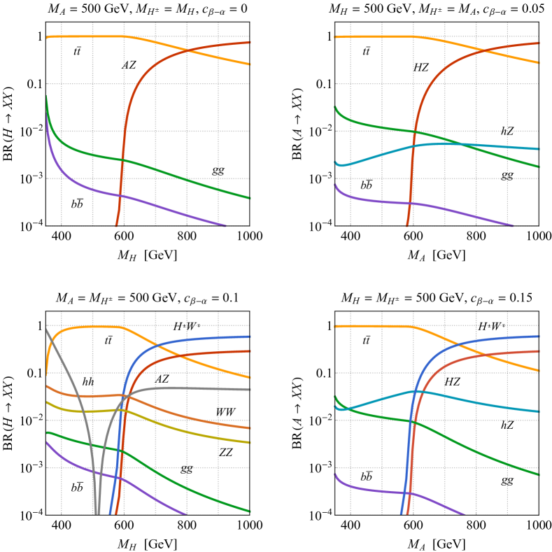
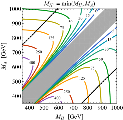
The above discussion suggests that close to the alignment limit the decay pattern of the heavy Higgses and is rather simple in all 2HDMs. To corroborate this statement we show in Figure 1 the branching ratios of and for four type-II 2HDM benchmark models. The different benchmarks thereby cover values of that range from the pure alignment limit to the case of maximally allowed misalignment, which amounts to around in the type-II 2HDM after LHC Run-1 (see for instance CMS (2016a)). Our calculation of the branching ratios is based on the formulas and results given in Djouadi et al. (1996); Djouadi (2008a, b); Alves et al. (2017); Haisch and Malinauskas (2018); Haisch et al. (2018). From the upper left panel one observes that for the decay almost fully saturates the total width of , while for the decay mode becomes important quickly and even dominant for . A similar picture arises in the case of the with and representing the two dominant decay modes for . This feature is illustrated in the upper right panel in Figure 1.
Notice that to obtain the latter plots we have fixed and , respectively. These choices are well-motivated, because only in these two cases Haber and Pomarol (1993); Pomarol and Vega (1994); Gerard and Herquet (2007); Grzadkowski et al. (2011); Haber and O’Neil (2011) can the or the have a sizeable mass splitting from the rest of the non-SM Higgses without being in conflict with EW precision measurements. The left (right) panel shown in the lower row of Figure 1 illustrate how the decay pattern of () changes if the charged Higgs mass is instead set equal to the mass of the heavy CP-odd (CP-even) Higgs. One observes that for such parameter choices besides and ( and ) also the channel () is important at high (). This feature is expected because () decays to a charged Higgs and a boson are kinematically allowed if () and unsuppressed in the alignment limit see (2). From the lower left panel one furthermore sees that for a non-zero value of the branching ratio of exceed the few-percent level for , making it the fourth largest branching ratio for heavy CP-even Higgses . We add that the results shown in the latter panel correspond to the choice , where is the quartic coupling that multiplies the term in the 2HDM scalar potential, and and denote the two Higgs doublets in the basis.
3 Anatomy of the signature
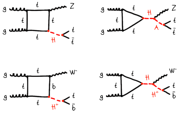
The discussion in the last section singles out the and final states as promising to search for the presence of heavy Higgs particles. Prototypes of Feynman diagrams that lead to the former signal in 2HDMs are shown in the upper row of Figure 2. In the graph on the left-hand side a is produced in association with a boson from a top-quark box, while in the right diagram the is emitted from a top-quark triangle and then decays via . Graphs where the role of the neutral Higgses and is interchanged also contribute to the signature in 2HDMs but are not explicitly shown in the figure.
In order to understand the anatomy of the signal in the 2HDM context, one first has to notice that the upper right Feynman diagram in Figure 2 allows for resonant production if the two conditions and are satisfied. Once the channels and are kinematically accessible the triangle graph therefore always dominates over the box contribution displayed on the upper left of the latter figure. In fact, the dominance of the triangle contribution allows one to estimate the signal strength . Since in the narrow-width approximation (NWA) the signal strength factorises into production and decay and given that for the parameters of interest, one obtains in the case of the following approximate result
| (4) |
If the signature arises instead through , the role of and has to simply be interchanged. The total production cross sections appearing in (4) are easy to calculate at leading order (LO). In the exact alignment limit and assuming that is not too large, we obtain at the following expressions
| (5) |
These approximations work to better than 20% for Higgs masses in the range of . They imply that the total production cross section of a is always larger than that of a if these particles have the same mass. For the relations (5) predict for example an enhancement factor of around 1.6. We emphasise that the formulas given in (5) serve mostly an illustrative purpose and have only been used to obtain the approximate signal strengths for and production as shown in Figures 3 and 5. Our numerical results presented in Section 8 and Appendices A and B instead do not use the approximations (5).
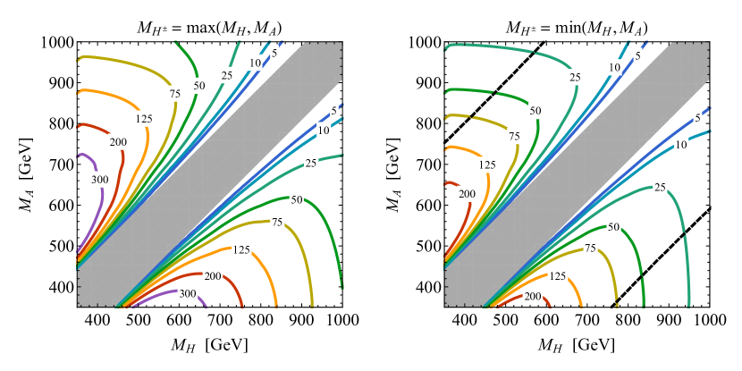
Figure 3 displays the signal strengths at as a function of and in the type-II 2HDM. The shown results are obtained by treating the process in the NWA. The kinematically inaccessible region in the – plane that separates (lower right corners) from (upper left corners) are indicated in grey. Both panels employ and . The left plot illustrates the choice meaning that the decay channels are closed. One sees that in this case the signal strength can reach and even exceed for and or vice versa. This number should be compared to the LO result for the SM production cross section at which amounts to . Notice that in accordance with (5) the signal strengths for are always slightly larger than those for . From the panel on the right-hand side of Figure 3 one moreover observes that the signal-over-background ratio is less favourable for the choice , because in this case the heavy neutral Higgses can decay to a charged Higgs and a boson. Despite this suppression, the signal strength can reach up to around , meaning that it still constitute a non-negligible fraction of the total SM production cross section. Notice that in the upper right (lower left) corner the width of the () becomes large because of () decays. To indicate this feature we have included in the figure dashed black contour lines that correspond to parameter choices leading to . For relative decay widths below the quoted value the NWA should be applicable.
The resonant contributions not only enhance the signal cross section, but also lead to interesting kinematic features that one can harness to discriminate signal from background. Firstly, since both heavy Higgses tend to be on-shell in the production chain , the invariant masses and of the and systems show characteristic Breit-Wigner peaks at
| (6) |
The difference between and can therefore be used to determine the mass splitting of the heavy Higgses. In the considered case, the distribution of the signal will for instance be peaked at
| (7) |
Second, since the four-momenta of the decay products and that enter are fixed by being preferentially on-shell, also the spectrum will have a characteristic shape. In fact, it is straightforward to show that the distribution of the resulting signal is a steeply rising function of with a cut-off at
| (8) |
that is smeared by the total decay width of the heavy Higgs . Needless to say, that the same line of reasoning and formulas similar to (6), (7) and (8) apply when one considers the process instead of .
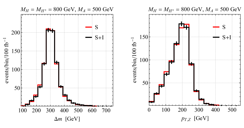
Figure 4 shows the and distribution that we obtain from a MadGraph5_aMCNLO Alwall et al. (2014) simulation of the new-physics contribution to the final state. The displayed results have been obtained in the context of the type-II 2HDM by employing a modified UFO implementation Degrande et al. (2012) of the 2HDM discussed in Bauer et al. (2017). The chosen parameters are , , and . The red predictions correspond to the pure new-physics signal (S), while the black distributions take into account the interference between the signal process and the background from SM production (). All relevant box and triangle diagrams have been included in our simulation. The distinctive kinematic features of the signal discussed earlier are clearly visible in the two panels with the distribution peaked at about and an edge in the spectrum at around . One also observes that, in contrast to the case of production Gaemers and Hoogeveen (1984); Dicus et al. (1994); Bernreuther et al. (1998); Frederix and Maltoni (2009); Hespel et al. (2016), signal-background interference leads only to minor distortions of the shapes of the most interesting distributions. Although the interference effects are observed to be small (roughly of the size of the statistical uncertainties in the shown example), we will include them in Section 8 when determining the sensitivity of the signature in constraining the parameter space of 2HDMs.
4 Anatomy of the signature
Two example diagrams that gives rise to a signal through the exchange of a charged Higgs boson are displayed in the lower row of Figure 2. In the left graph a and a are radiated off a box diagram with internal top and bottom quarks, while in the diagram on the right-hand side a is emitted from a top-quark triangle which then decays via . In both cases the charged Higgs boson decays to a pair. Notice that diagrams with or exchange also lead to a signal. These contributions while not explicitly shown in the lower row of Figure 2 are all included in our analysis.
The final state can be resonantly produced via () followed by the decay if the two conditions () and are fulfilled. In such a case triangle diagrams provide the leading contribution to the signal strength. In Figure 5 we show at in the – plane, treating the process in the NWA. The depicted results correspond to the type-II 2HDM and , and . The regions of parameter space in which the new-physics signal arises from (lower right corner) or from (upper left corner) are divided by a grey stripe that masks Higgs masses satisfying . From the figure one observes that the signal strength can be as large as (or even larger) for and . Since for the total production cross section is bigger than , one again notices a small asymmetry between the signal strengths and with the former being always slightly larger than the latter.
Like the case of the signal, also the kinematic distributions of the signature have distinctive features that can be exploited to tame SM backgrounds. Figure 6 shows an assortment of invariant mass distributions that can serve this purpose. The displayed results have been obtained in the type-II 2HDM using MadGraph5_aMCNLO. The choice of parameters is , , and . The left panel in the upper row of the figure depicts the invariant mass of the system in . One sees that the distribution has a sharp edge at around , which corresponds to the kinematic endpoint Allanach et al. (2000); Lester and Parker (2001)
| (9) |
Similarly, also the invariant mass of the final-state configuration that appears in the channel from the sequential decay has a kinematic endpoint. It is located at Allanach et al. (2000); Lester and Parker (2001)
| (10) |
The associated edge in the spectrum arises at about , a feature that is evident in the upper right panel of Figure 6. Notice that final states also arise from the leptonic decay of the bosons involved in . The corresponding invariant mass has a very soft endpoint at and no edge because the lepton is not emitted directly from the backbone of the whole decay chain. Since experimentally one can separate the two cases (see Section 7), an example of a signal distribution has not been depicted in Figure 6.
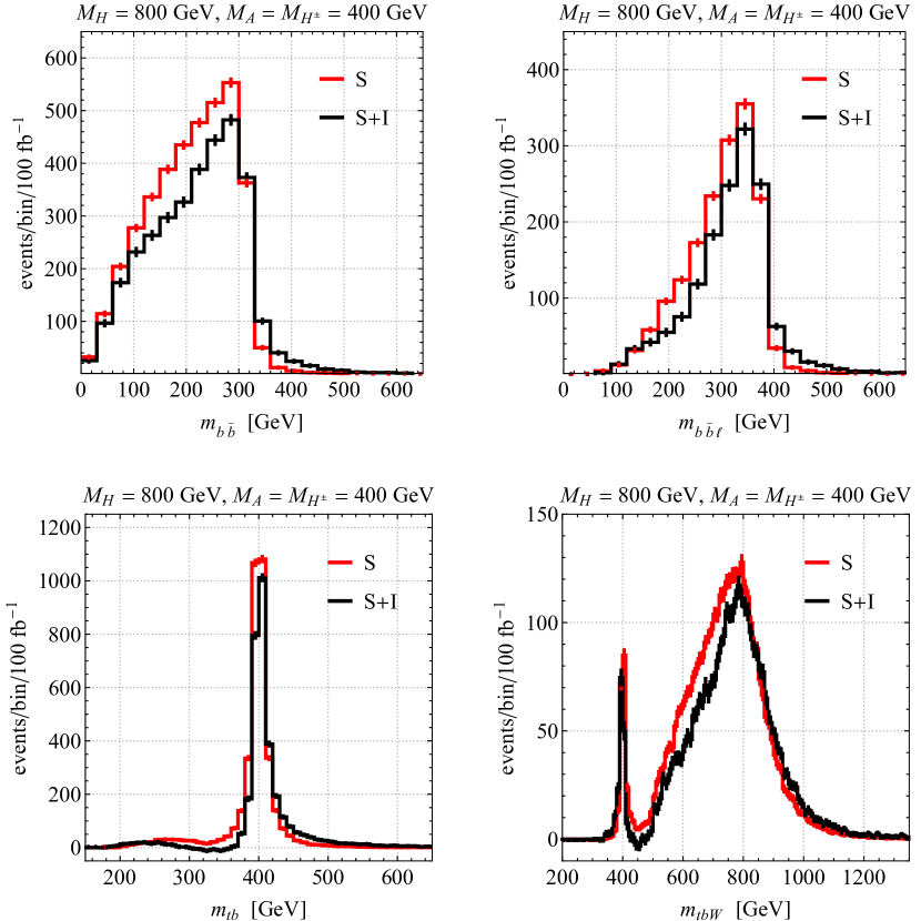
In the lower left panel the invariant mass of the system is depicted. As expected, this distribution shows a Breit-Wigner peak at
| (11) |
The invariant mass of the final state is displayed in the lower right panel of Figure 6. The two mass peaks at
| (12) |
resulting from and , respectively, are clearly visible in the figure. Notice that the peak at approximately is smeared by the total decay width of the heavy Higgs which in the case at hand amounts to . The resonance peak centred at is on the other hand narrow since .
Realise that not only the process (example diagrams are shown in the lower row of Figure 2) but also graphs corresponding to contribute to the signature in 2HDMs. To separate the charged Higgs contributions to the channel from the neutral Higgs contributions associated to production, we employ the so-called diagram removal (DR) procedure Frixione et al. (2008). In this scheme the final state is defined by removing from the scattering amplitude all doubly resonant diagrams, i.e. graphs in which the intermediate top quarks can be on-shell. Singly resonant contributions are on the other hand kept. The DR procedure is also applied to the SM amplitudes, and as a result only -fusion (but no top-fragmentation) diagrams contribute at LO in QCD to the final state.
Based on the DR definition of the final state, we have studied the impact of signal-background interference. The red curves in Figure 6 correspond to the pure new-physics signal (S), while the black distributions in the four panels take into account the interference between the signal process and the background from production within the SM (). Comparing the two sets of histograms, we observe that the kinematic features in the , , and distributions are always less pronounced for the predictions than the S results. Since the size of the signal-background interference typically exceeds the statistical uncertainties expected in future LHC runs, a rigorous assessment of the prospects of the final state to search for heavy Higgses should be based on MC simulations that include interference effects between the new-physics signal and the SM background.
5 MC generation and detector simulation
In our study we consider throughout collisions at . We generate the signal samples using a modified version of the Pseudoscalar_2HDM UFO together with MadGraph5_aMC@NLO and NNPDF23_lo_as_0130 parton distribution functions Ball et al. (2013). Compared to the UFO presented in Bauer et al. (2017) our new implementation is able to calculate the interference between the loop-induced and signals and the corresponding tree-level SM backgrounds. The obtained parton-level events are then decayed and showered with PYTHIA 8.2 Sjöstrand et al. (2015) which allows us to study the fully interfered signals and backgrounds at the detector level.
Our analysis will address the three-lepton final state, with two opposite-sign same-flavour leptons from the -boson decay and one lepton from the semileptonic decay of one of the two top quarks. For the description of the SM backgrounds to this final state, SM processes involving at least three leptons coming from the decay of EW gauge bosons are simulated. Most of the backgrounds are generated at LO with MadGraph5_aMC@NLO. The dominant irreducible background is which is generated with up to an additional jet. The background is instead generated with up to two additional jets. The dominant diboson background, i.e. , is simulated with up to three additional jets. The minor backgrounds considered are and both of which are obtained using MadGraph5_aMC@NLO. In each case the decay of the top quarks and the EW gauge bosons is performed by MadGraph5_aMC@NLO. The reducible background is generated at next-to-leading order (NLO) with POWHEG BOX Alioli et al. (2010).
A potential significant background in the case of the channel arises from processes where two leptons are produced in the decays of EW gauge bosons, and a third lepton is either the result of a misidentification in the detector or the decay of a meson. The latter is experimentally strongly suppressed by requiring the leptons to be isolated. The estimate of these backgrounds requires a profound understanding of the detector performance, and indeed the ATLAS and CMS use data-driven techniques rather than MC simulations to determine them. A recently published search for by the ATLAS experiment Aad et al. (2015b) shows that the requirement of having at least four jets of which two are identified as coming from the fragmentation of bottom quarks reduces the background from misidentified leptons to a level well below the other backgrounds.
In the case of the analysis, the background evaluation is performed through the generation of SM processes involving at least two leptons coming from the decays of EW gauge bosons. The backgrounds from Campbell et al. (2015), Re (2011), , and production Melia et al. (2011); Nason and Zanderighi (2014) were all generated at NLO with POWHEG BOX. The sample is generated at LO with MadGraph5_aMC@NLO, considering up to four jets for the matrix element calculation. The latter MC code is also used to simulate the backgrounds with at LO with a multiplicity of up to two jets, and the and backgrounds at LO. As for the analysis, we do not consider final states where one or both of the leptons are either fake electrons from jet misidentification or real non-isolated leptons from the decay of heavy flavours.
All partonic events are showered with PYTHIA 8.2 and the SM backgrounds are normalised to their NLO cross section calculated either with MadGraph5_aMC@NLO or with POWHEG BOX where relevant. The simulated analyses are performed on experimentally identified electrons, muons, photons, jets and which are constructed from the stable particles in the generator output. Jets are constructed by clustering the true momenta of all the particles interacting in the calorimeters, with the exception of muons. An anti- algorithm Cacciari et al. (2008) with a parameter is used, as implemented in FastJet Cacciari et al. (2012). Jets originating from the hadronisation of bottom quarks (-jets) are experimentally tagged in the detector (-tagged). The variable with magnitude is defined at truth level, i.e. before applying detector effects, as the vector sum of the transverse momenta of all the invisible particles (neutrinos in our case). The effect of the detector on the kinematic quantities used in the analysis is simulated by applying a Gaussian smearing to the momenta of the different reconstructed objects and reconstruction and tagging efficiency factors. The parametrisation of the smearing and of the reconstruction and tagging efficiencies is tuned to mimic the performance of the ATLAS detector Aad et al. (2008, 2009) and is applied as a function of the momentum and the pseudorapidity of the physical objects. The discrimination of the signal from the background is significantly affected by the experimental smearing assumed for . To simulate this effect, the transverse momenta of unsmeared electrons, muons and jets are subtracted from the truth and replaced by the corresponding smeared quantities. The residual truth imbalance is then smeared as a function of the scalar sum of the transverse momenta of the particles not assigned to electrons or jets. The same techniques have also been employed in Haisch et al. (2017); Pani and Polesello (2018).
6 Analysis strategy for the signature
In the case of the channel the generated signal and background events are preselected by requiring exactly three charged leptons (electrons or muons) with a pseudorapidity of . The leading lepton must have , while the other two are required to satisfy . At least one pair of leptons of opposite charge and same flavour must be present, and the invariant mass of this pair must meet the requirement . In case the event includes more than one such lepton pair, the pair with the invariant mass closest to the nominal value of is selected as the -boson candidate. All events furthermore need to contain four jets with and , of which two must be tagged as bottom-quark jets (-tagged).
Notice that the large jet multiplicity and the requirement of having two -tagged jets leads, on the one hand, to a strong reduction of the and SM backgrounds, and on the other selects all objects needed for a full reconstruction of the event. The leptonically decaying boson is reconstructed from the charged lepton not assigned to and the amount of by solving the -boson mass constraint. If the solution for the longitudinal momentum of the neutrino is imaginary, the real part of is taken. The reconstructed jets are assigned to the different and top decays, by choosing the assignment which gives the best compatibility with the decay of two top quarks in terms of reconstructed masses. If in the process two solutions are found for the reconstructed leptonic decay, the one giving the best mass compatibility is selected.
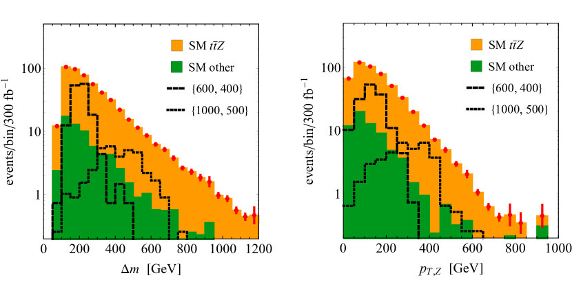
In Figure 7 the distributions of and for the SM backgrounds and two type-II 2HDM benchmark models after applying the selections described above are displayed. Our benchmarks correspond to , (, ), and and are indicated by the dashed (dotted) black lines. In the case of the spectrum, one observes from the left panel that the sum of the SM backgrounds is a steeply falling distribution, while both new-physics signals exhibit a Breit-Wigner peak. In fact, as expected from (7) the peaks are located at around and . Our results for the distributions are presented in the right panel of the latter figure. In agreement with (8) the two 2HDM benchmark models lead to spectra that show distinctive Jacobian peaks with edges at roughly and . The SM backgrounds are in contrast again smoothly falling and featureless. Notice that a measurement of the distribution in production does, unlike a measurement of the difference of invariant masses, not require the full reconstruction of the final state. As a result, is less subject to experimental uncertainties than . In order to stress the experimental robustness of the proposed signature, we will in our sensitivity study consider both the and the distribution as final discriminants.
7 Analysis strategy for the signature
In the case of the signal the dominant QCD backgrounds are production and production in association with a -jet. By vetoing events where the observed bosons and -jets are kinematically compatible with the decay of two top quarks the overwhelming background can be reduced by approximately two orders of magnitude, making it comparable to the background in size. After this selection the signal is however still two orders of magnitude smaller than the background. Notice that this is in contrast to the channel where the signal and the background are of the same size after background suppression. To improve the signal-over-background ratio in the case of the signal, one needs to exploit the decay kinematics of the heavy Higgses by identifying the decay products of the top quark in the signal events. The invariant mass of the top quark with the additional -jet will be peaked at , while the invariant mass of the two -jets and the two bosons equals or depending on which mass is larger. Experimentally the signal can be looked for in events with two, one or zero isolated charged leptons resulting from . In the following we will sketch a possible analysis procedure for the two-lepton final state. Given the small signal-to-background ratio for the irreducible backgrounds, we however expect that our conclusions will be valid for the one-lepton final state as well.
For the two-lepton case, the reconstruction of mass peaks is not possible due to the presence of two neutrinos in each event. However, given the presence of multi-step sequential decays leading to undetected neutrinos, the invariant mass distributions of the visible decay products are bounded from above Hinchliffe et al. (1997). In the case of top decays, the invariant mass of the resulting -quark and lepton must be lower than . Thus exactly two opposite-sign leptons ( and ) with and and exactly two -tagged jets ( and ) with are required in the event, and events are selected in which none of the two possible pairings among -jets and leptons is compatible with the decay of two top quarks. A convenient way of rejecting events compatible with two top decays consists in introducing the observable
| (13) |
where the minimisation runs over all pairs of distinct jets inside a predefined set of test jets. Based on the number of -tagged jets in the event, the set of test jets is defined as follows. If the event includes one or two -tagged jets, an additional test jet is considered, chosen as the non--tagged jet with the highest -tagging weight and . If three -tagged jets are found, they are all taken as test jets. The requirement suppresses the background by approximately two orders of magnitude. A dangerous background is also also due to the production of a boson in association with -jets. Vetoing same-flavour lepton pairs compatible with a -boson decay and requiring some reduces this background to roughly the level of the signal, albeit with large uncertainties. To avoid this possible issue we completely remove the latter and all other backgrounds including a real boson by requiring that the two selected leptons have different flavours. After these selections the remaining background consists of approximately one half of and one half of events.
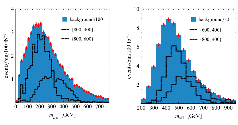
A further separation of signal from background can be achieved by exploiting the fact that in the case of the signal the invariant mass of the two -tagged jets as well as the invariant mass of the two -tagged jets with the lepton from a top decay are bounded from above. See (9) and (10). In order to illustrate this point we show in the left panel of Figure 8 the distribution of for two signal samples with (dashed black line) and (dotted black line), respectively. The remaining 2HDM parameters are set to , and and the background has been scaled down by a factor of 100 for better visibility. Upper cuts on matching the kinematic endpoint of the signal for different values of will improve the signal-over-background ratio, bringing it to a level of at most 3% over the parameter space relevant for this analysis. The variable is less effective as it has a less sharp edge, and suffers from an ambiguity in the choice of the lepton.
The final experimental handle is the fact that the invariant mass of the system will peak at the mass of the bosons for the bulk of the signal (cf. Figure 6) whereas for the background has a broad distribution centred at around . However, if the charged Higgs mass is not known, the observable cannot be reconstructed because of the two undetected neutrinos. A large literature on the reconstruction of the mass of new particles in events with two invisible particles in the final state is available (see e.g. Gripaios (2011) for a review). In our exploratory study, we employ the variable as an estimator of , which is defined as Paige (1996); Hinchliffe et al. (1997)
| (14) |
In the right panel of Figure 8 we show the distribution for (dashed black line) and (dotted black line), fixing the other parameters to , and . For better visibility the background has been scaled down by a factor 50 after applying the cut . The significance of the signal can be extracted from a shape fit to the spectrum for signal and background. Given the difference in shape between signal and background, and the large number of kinematic handles, it should be possible to extract a significant signal for a signal sample corresponding to 3 ab-1 of integrated luminosity if the shape of the background can be experimentally controlled to a level below . In these conditions a reliable evaluation of the coverage in parameter space can only be performed by the experimental collaborations. It is however worth noting that, due to the shape of the background distribution, the maximum sensitivity of the analysis is expected to arise for , making the coverage complementary to that of the search.
8 Numerical results
Based on the search strategy outlined in Section 6, we now study the sensitivity of future LHC runs to the signature. To evaluate the upper limit on the ratio of the signal yield to that predicted in the 2HDM framework, a profiled likelihood ratio test statistic applied to the shapes of the and distributions is used. The CLs method Read (2002) is employed to derive exclusion limits at 95% confidence level (CL). The statistical analysis has been performed by employing the RooStat toolkit Moneta et al. (2010). A systematic uncertainty on the absolute normalisation of the SM background (signal) of 15% (5%) is assumed. This choice of uncertainties is in accordance with the uncertainties obtained by ATLAS and CMS for existing searches in similar final states. For the signal, the main uncertainty is generated by the impact on the selection efficiency of uncertainties on the measurement of quantities such as e.g. the energy scale and resolution for jets and . In the case of the background there is in addition an important contribution to the total uncertainty that is associated with the procedure used to obtain the background estimate, which is typically achieved through a mixture of MC and data-driven techniques. Since we perform a shape analysis, the obtained fit results have reduced sensitivity to the absolute normalisation uncertainties, and are essentially determined by the uncertainties on the prediction of the shape of the distribution of the fitted variable for the SM background. The magnitude of these uncertainties is difficult to forecast, as they include different factors, such as the shape distortion from uncertainties on energy and efficiency determinations, or theoretical uncertainties associated to the simulation of the background. A variety of techniques are used by the experiments to control shape uncertainties, including the usage of appropriate control regions and the profiling of experimental uncertainties. In the case of the final state, shape uncertainties of a few percent seem to be an achievable goal, and we will determine the LHC reach, assuming a representative value of for the latter uncertainty.
The results given in the following are for integrated luminosities of and , corresponding to the LHC Run-3 phase and the high-luminosity option of the LHC (HL-LHC), respectively. As the LHC experimental community is still working on the detailed assessment of the impact of the high pileup on the detector performance in the HL-LHC phase, we assume for simplicity the same detector performance for the two benchmark luminosities. The analysis based on the variable, relying on an accurate measurement of and the momenta of jets will likely be affected by pileup. In contrast, we expect only a minor impact on the variable, built from two high- leptons. Under the assumptions presented above, we find that a shape analysis using leads to only marginally better results than a fit to . We are therefore convinced that the conclusions of this study are valid also in the presence of a much higher pileup than the one experienced in the ongoing LHC run. In this section, we will only show the results of our shape fit. A comparison of the performance of the and fits is provided in Appendix A.
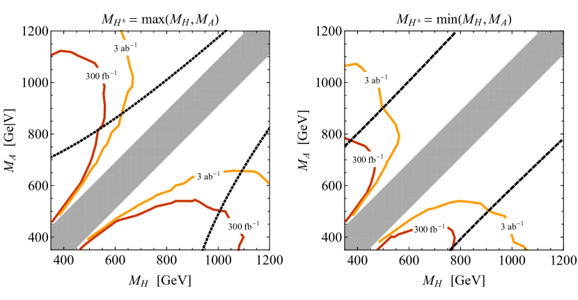
The results of our sensitivity study are displayed in Figures 9 and 10. In the two panels of the first figure, we show the 95% CL exclusion limits in the – plane that derive from a shape fit to the observable introduced in (7). The red (yellow) contours illustrate the constraints that follow from of data collected at . They are obtained in the type-II 2HDM employing , , (left panel) and (right panel). The region in the – plane that is kinematically inaccessible is indicated in grey. From the red contours in the left plot, one sees that if the intermediate can only decay to the final state but not to , based on the entire LHC Run-3 data set it should be possible to exclude masses in the range of approximately () for (). If, on the other hand, the decay channels are open, the exclusion reduces to for as illustrated by the red contour lines in the right panel. It is also evident from the two panels, that with of data that the HL-LHC is expected to collect, it may be possible to improve the LHC Run-3 sensitivity by up to a factor of 1.5. The corresponding contours are coloured yellow in Figure 9. The improvements are more pronounced for than for , and numerically largest for mass hierarchies . Notice that in these cases the signal strengths are small and in consequence the proposed search is statistics limited at LHC Run-3. The discovery reach corresponding to Figure 9 can be found in Appendix B.
At this point, one should mention that large mass splittings between the heavy Higgses are in general constrained by theoretical arguments such as perturbativity and vacuum stability. In order to illustrate this point, we depict in the left panel of Figure 9 the parameter space that is disfavoured by requiring simultaneously the quartic coupling to be perturbative, i.e. , and the simplest 2HDM scalar potential to be bounded from below Gunion and Haber (2003). The displayed constraints can be relaxed in more general 2HDMs containing additional quartic couplings like for example , and the shown contours should therefore only be considered as indicative, having the mere purpose to identify theoretically (dis)favoured parameter regions (see Bauer et al. (2018) for a more detailed discussion of this point). In the right plot in Figure 9, perturbativity and vacuum stability arguments instead do not lead to any restriction on the shown parameter space. As discussed before, in this case the total decay width of () however becomes large because the () channel is open. The family of values that leads to is indicated by the dashed black lines in the right panel. Although our analysis is performed keeping effects due to off-shell production and decay, and due to the interference with the SM background (see Section 3), it ignores possible modifications of the line shape Seymour (1995); Goria et al. (2012); Passarino et al. (2010). The latter effects have been studied in Anastasiou et al. (2011, 2012), where it was found that for a heavy Higgs boson different treatments of its propagator can lead to notable changes in the inclusive production cross sections compared to the case of a Breit-Wigner with a fixed width, as used in our work. In consequence, the exclusion limits in the upper left and lower right corner of the right plot in Figure 9 carry some (hard to quantify) model dependence related to the precise treatment of the propagators.
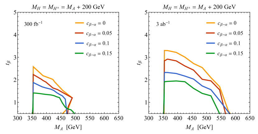
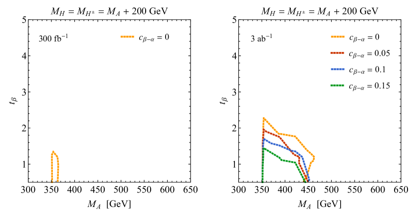
In Figure 10 we show furthermore the 95% CL exclusion contours in the – plane for the type-II 2HDM scenarios with and . In both panels the results of our shape fit are given for four different values of . Notice that for the chosen parameters there are no issues with perturbativity and vacuum stability, and that the is sufficiently narrow for the NWA to hold. From the results shown on the left-hand side one observes that with of data, all values of can be excluded for masses close to the top threshold in the exact alignment limit, i.e. . If the Higgs sector is not perfectly aligned, the branching ratio is reduced see (2), and as a result the bounds in the – plane become weaker. For instance, for the choice , we find that the reach is decreased by roughly a factor of 1.5 compared to the case of full alignment. One also sees that values up to around can be excluded with for and . With of integrated luminosity it turns out that the obtained limits can be pushed to values of and that are higher by approximately than the corresponding bounds. This statement is illustrated by the coloured contours that are displayed in the right panel of Figure 10. The discovery reach corresponding to the latter figure are provided in Appendix B.
The constraints on the type-II 2HDM parameter space presented in this section should be compared to the bounds that have been derived in Craig et al. (2015); Hajer et al. (2015); Gori et al. (2016). These analyses have considered the , and channels, and there seems to be a consensus that future searches for should provide the best sensitivity to neutral Higgses with masses at low values of . While a one-to-one comparison with the exclusions obtained in Craig et al. (2015); Hajer et al. (2015); Gori et al. (2016) is not possible, we note that the limits derived in our work appear to be more stringent than the bounds reported in the latter articles. In this context it is important to realise that the reach of the searches has found to be strongly dependent on the systematic uncertainty of the normalisation of the background. The analysis strategy proposed by us does in contrast not rely on knowing the absolute size of the relevant backgrounds to the level of a few percent, since the search gains its discriminating power from shape differences. We therefore expect future searches to lead to the most robust coverage of the 2HDM parameter space with , and .
9 Conclusions
In this article, we have proposed to use the and final states to search for heavy Higgs bosons at the LHC. These final states are interesting, because in the 2HDM context they can arise resonantly from or , if the requirements and or and are satisfied. In fact, the involved couplings , , , , and are all non-vanishing for see (2) and (3) which corresponds to the so-called alignment limit that is experimentally favoured by the agreement of the LHC Higgs measurements with SM predictions. As a result, appreciable and rates associated to production turn out to be a rather generic prediction in 2HDMs that feature a SM-like scalar and non-SM Higges that are heavier than about with some of their masses split by around or more.
By analysing the anatomy of the and signatures in 2HDMs, we have demonstrated that many of the resulting final-state distributions show peaks and/or edges that are characteristic for the on-shell production of a resonance followed by its sequential decay into visible and invisible particles. These kinematic features can be used to disentangle the new-physics signal from the SM background. In the case of the final state, we found that the difference between the masses of the and systems and the transverse momentum of the boson are powerful discriminants, while in the case of the final state the invariant masses , , and can be exploited for a signal-background separation. Our MC simulations have furthermore shown that the discussed observables can all be reconstructed and well measured under realistic experimental conditions through either a dedicated three-lepton ( and ) or two-lepton ( and ) analysis strategy (see Sections 6 and 7).
Applying our three-lepton analysis strategy to simulated 14 TeV LHC data, we have then presented a comprehensive sensitivity study of the signature in the 2HDM framework. We have derived various 95% CL exclusion limits on the parameter space of the type-II 2HDM that follow from a shape fit to the (see Section 8) and (see Appendix A) distributions. Our analysis shows that for the parameter choices , , and assuming of integrated luminosity, it should be possible to exclude all mass combinations inside a roughly triangular region spanned by the points , and . In the case of the mass hierarchy the decays are open and we instead find that the exclusions only reach up to around and (see Figure 9). For the scenarios , we have also derived the 95% CL exclusion limits in the – plane for four different values of (see Figure 10). For the choice , we found for instance that it should be possible to exclude values up to almost 2 for , assuming of data. The HL-LHC is expected to improve the quoted LHC Run-3 limits noticeably. The discovery reach in the – and – plane can be found in Appendix B. The constraints obtained in our work are complementary to and in many cases stronger than the exclusions that future LHC searches for the processes , and are expected to be able to provide (cf. Craig et al. (2015); Hajer et al. (2015); Gori et al. (2016)) on 2HDMs with neutral Higgses with and small values of .
In the case of the final state, we have found that for both the two-lepton and one-lepton analysis the signal-over-background ratios do not exceed the level of a few percent. As a result, a reliable evaluation of the coverage of the 2HDM parameter space would require to make strong assumptions about the systematic uncertainties that plague the normalisation and shape of the background at future LHC searches. Since we feel that it would be premature to make these assumptions, we hope that the ATLAS and CMS collaborations will explore the signature further. This is a worthwhile exercise, because we expect that at the HL-LHC with of integrated luminosity, this channel should also allow to probe parts of the 2HDM parameter space that feature heavy non-SM Higgses and values of the order of a few. In fact, the maximum sensitivity of our analysis arises for , making the coverage complementary to that of the proposed search.
Acknowledgements.
We are grateful to Stefania Gori and Priscilla Pani for useful conversations, and would like to thank Valentin Hirschi and Eleni Vryonidou for help with MadGraph5_aMCNLO. UH acknowledges the continued hospitality and support of the CERN Theoretical Physics Department.Appendix A Shape analysis using
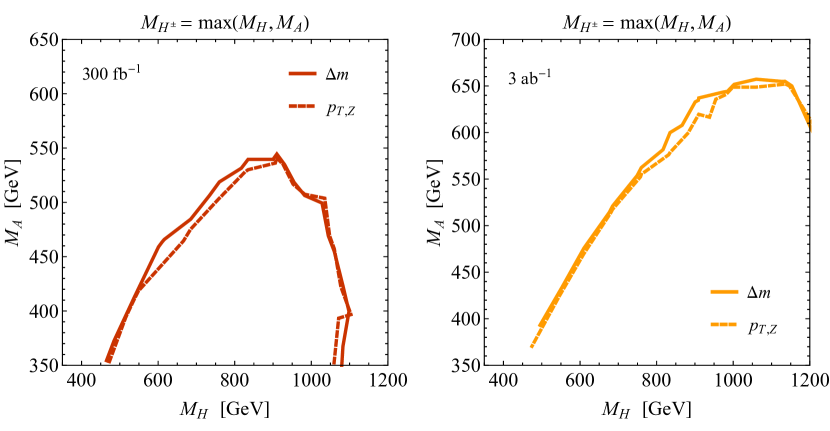
The 95% CL exclusions shown in Section 8 have been obtained from a shape analysis of the variable (7). Since the measurement of relies on accurate measurements of and the momenta of jets it will likely be affected by the large pileup present in the HL-LHC phase. In contrast, pileup is expected to have only a minor impact on , because this observable can be reconstructed from the measurement of two charged leptons with high transverse momentum. To corroborate the statement made in Section 8 that our analysis strategy is robust with respect to pileup, we compare in Figure 11 the performance of the proposed and shape analyses. The given results are obtained in the type-II 2HDM employing , , and only the parameter space with is shown. The assumptions about the uncertainties entering our analyses are specified in Section 8. One observes that a shape analysis based on (solid contours) leads to only marginally better 95% CL exclusions than a fit using (dashed contours) at both (left panel) and (right panel). This observation makes us confident that the main conclusions of this work also hold in the presence of the large pileup expected at the HL-LHC.
Appendix B Discovery reach
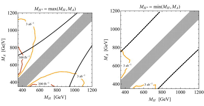
In this appendix we extend the numerical study performed in Section 8 by presenting the discovery reach corresponding to Figures 9 and 10. The limits in the – plane that stem from our shape fit are shown in Figure 12. The dotted red (dotted yellow) contours correspond to of integrated luminosity at . The displayed limits are obtained in the type-II 2HDM using , , (left panel) and (right panel). The part in the – plane that is kinematically inaccessible is shaded grey. One observes that the full LHC Run-3 has a quite limited discovery reach, as it can achieve significance only for masses in the range of around assuming that and . Furthermore, in the case of no discovery seems possible with of data. The situation is however expected to improve significantly with of integrated luminosity. In the case of , we find that the HL-LHC may be able to discover all mass combinations inside a region spanned by the points , and , while for only heavy neutral Higgs bosons with masses in the range of can potentially be discovered if . Notice that the quoted HL-LHC limits are similar to the 95% CL exclusions obtained in Section 8 for LHC Run-3.
Figure 13 displays in addition the discovery reach in the – plane for the type-II 2HDM scenarios with , and four different values of . From the results obtained for of data (left panel) one can see that a discovery seems only possible in the exact alignment limit for and masses close to the top threshold. The discovery reach is again significantly improved at the HL-LHC with of integrated luminosity (right panel), which should be able to achieve a significance of for all scenarios with in the range of approximately , and .
References
- Aad et al. (2012) G. Aad et al. (ATLAS), Phys. Lett. B716, 1 (2012), arXiv:1207.7214 [hep-ex] .
- Chatrchyan et al. (2012) S. Chatrchyan et al. (CMS), Phys. Lett. B716, 30 (2012), 1207.7235 .
- Sirunyan et al. (2017a) A. M. Sirunyan et al. (CMS), JHEP 11, 047 (2017a), arXiv:1706.09936 [hep-ex] .
- Aaboud et al. (2017a) M. Aaboud et al. (ATLAS), JHEP 10, 132 (2017a), arXiv:1708.02810 [hep-ex] .
- Aaboud et al. (2018a) M. Aaboud et al. (ATLAS), (2018a), arXiv:1802.04146 [hep-ex] .
- Sirunyan et al. (2018a) A. M. Sirunyan et al. (CMS), (2018a), arXiv:1804.02716 [hep-ex] .
- Aad et al. (2016) G. Aad et al. (ATLAS, CMS), JHEP 08, 045 (2016), arXiv:1606.02266 [hep-ex] .
- Aad et al. (2015a) G. Aad et al. (ATLAS), JHEP 11, 206 (2015a), arXiv:1509.00672 [hep-ex] .
- CMS (2016a) Summary results of high mass BSM Higgs searches using CMS run-I data, Tech. Rep. CMS-PAS-HIG-16-007 (CERN, Geneva, 2016).
- Aaboud et al. (2018b) M. Aaboud et al. (ATLAS), JHEP 01, 055 (2018b), arXiv:1709.07242 [hep-ex] .
- Sirunyan et al. (2018b) A. M. Sirunyan et al. (CMS), JHEP 09, 007 (2018b), arXiv:1803.06553 [hep-ex] .
- Khachatryan et al. (2015a) V. Khachatryan et al. (CMS), JHEP 11, 071 (2015a), arXiv:1506.08329 [hep-ex] .
- CMS (2016b) Search for a narrow heavy decaying to bottom quark pairs in the 13 TeV data sample, Tech. Rep. CMS-PAS-HIG-16-025 (CERN, Geneva, 2016).
- Sirunyan et al. (2018c) A. M. Sirunyan et al. (CMS), JHEP 08, 113 (2018c), arXiv:1805.12191 [hep-ex] .
- Khachatryan et al. (2015b) V. Khachatryan et al. (CMS), JHEP 10, 144 (2015b), arXiv:1504.00936 [hep-ex] .
- Aaboud et al. (2018c) M. Aaboud et al. (ATLAS), Eur. Phys. J. C78, 24 (2018c), arXiv:1710.01123 [hep-ex] .
- Aaboud et al. (2018d) M. Aaboud et al. (ATLAS), JHEP 03, 009 (2018d), arXiv:1708.09638 [hep-ex] .
- Aaboud et al. (2018e) M. Aaboud et al. (ATLAS), Eur. Phys. J. C78, 293 (2018e), arXiv:1712.06386 [hep-ex] .
- Sirunyan et al. (2018d) A. M. Sirunyan et al. (CMS), JHEP 06, 127 (2018d), arXiv:1804.01939 [hep-ex] .
- Khachatryan et al. (2016a) V. Khachatryan et al. (CMS), Phys. Lett. B759, 369 (2016a), arXiv:1603.02991 [hep-ex] .
- CMS (2016c) Search for with 2015 data, Tech. Rep. CMS-PAS-HIG-16-010 (CERN, Geneva, 2016).
- Aaboud et al. (2018f) M. Aaboud et al. (ATLAS), Phys. Lett. B783, 392 (2018f), arXiv:1804.01126 [hep-ex] .
- Aaboud et al. (2018g) M. Aaboud et al. (ATLAS), JHEP 03, 174 (2018g), arXiv:1712.06518 [hep-ex] .
- Khachatryan et al. (2016b) V. Khachatryan et al. (CMS), Phys. Lett. B755, 217 (2016b), arXiv:1510.01181 [hep-ex] .
- ATL (2016) Search for Higgs boson pair production in the final state of () using 13.3 fb-1 of collision data recorded at 13 TeV with the ATLAS detector, Tech. Rep. ATLAS-CONF-2016-071 (CERN, Geneva, 2016).
- Sirunyan et al. (2018e) A. M. Sirunyan et al. (CMS), JHEP 08, 152 (2018e), arXiv:1806.03548 [hep-ex] .
- Khachatryan et al. (2017) V. Khachatryan et al. (CMS), Phys. Lett. B767, 147 (2017), arXiv:1609.02507 [hep-ex] .
- Aaboud et al. (2017b) M. Aaboud et al. (ATLAS), Phys. Lett. B775, 105 (2017b), arXiv:1707.04147 [hep-ex] .
- Aaboud et al. (2017c) M. Aaboud et al. (ATLAS), JHEP 10, 112 (2017c), arXiv:1708.00212 [hep-ex] .
- Sirunyan et al. (2017b) A. M. Sirunyan et al. (CMS), (2017b), arXiv:1712.03143 [hep-ex] .
- Djouadi et al. (2015) A. Djouadi, L. Maiani, A. Polosa, J. Quevillon, and V. Riquer, JHEP 06, 168 (2015), arXiv:1502.05653 [hep-ph] .
- Craig et al. (2015) N. Craig, F. D’Eramo, P. Draper, S. Thomas, and H. Zhang, JHEP 06, 137 (2015), arXiv:1504.04630 [hep-ph] .
- Hajer et al. (2015) J. Hajer, Y.-Y. Li, T. Liu, and J. F. H. Shiu, JHEP 11, 124 (2015), arXiv:1504.07617 [hep-ph] .
- Gori et al. (2016) S. Gori, I.-W. Kim, N. R. Shah, and K. M. Zurek, Phys. Rev. D93, 075038 (2016), arXiv:1602.02782 [hep-ph] .
- Alvarez et al. (2017) E. Alvarez, D. A. Faroughy, J. F. Kamenik, R. Morales, and A. Szynkman, Nucl. Phys. B915, 19 (2017), arXiv:1611.05032 [hep-ph] .
- Aaboud et al. (2017d) M. Aaboud et al. (ATLAS), Phys. Rev. Lett. 119, 191803 (2017d), arXiv:1707.06025 [hep-ex] .
- Sirunyan et al. (2018f) A. M. Sirunyan et al. (CMS), Eur. Phys. J. C78, 140 (2018f), arXiv:1710.10614 [hep-ex] .
- Aaboud et al. (2018h) M. Aaboud et al. (ATLAS), (2018h), arXiv:1803.09678 [hep-ex] .
- Gaemers and Hoogeveen (1984) K. J. F. Gaemers and F. Hoogeveen, Phys. Lett. 146B, 347 (1984).
- Dicus et al. (1994) D. Dicus, A. Stange, and S. Willenbrock, Phys. Lett. B333, 126 (1994), arXiv:hep-ph/9404359 [hep-ph] .
- Bernreuther et al. (1998) W. Bernreuther, M. Flesch, and P. Haberl, Phys. Rev. D58, 114031 (1998), arXiv:hep-ph/9709284 [hep-ph] .
- Frederix and Maltoni (2009) R. Frederix and F. Maltoni, JHEP 01, 047 (2009), arXiv:0712.2355 [hep-ph] .
- Hespel et al. (2016) B. Hespel, F. Maltoni, and E. Vryonidou, JHEP 10, 016 (2016), arXiv:1606.04149 [hep-ph] .
- Glashow and Weinberg (1977) S. L. Glashow and S. Weinberg, Phys. Rev. D15, 1958 (1977).
- Paschos (1977) E. A. Paschos, Phys. Rev. D15, 1966 (1977).
- Craig et al. (2013) N. Craig, J. Galloway, and S. Thomas, (2013), arXiv:1305.2424 [hep-ph] .
- Djouadi et al. (1996) A. Djouadi, J. Kalinowski, and P. M. Zerwas, Z. Phys. C70, 435 (1996), arXiv:hep-ph/9511342 [hep-ph] .
- Djouadi (2008a) A. Djouadi, Phys. Rept. 457, 1 (2008a), arXiv:hep-ph/0503172 [hep-ph] .
- Djouadi (2008b) A. Djouadi, Phys. Rept. 459, 1 (2008b), arXiv:hep-ph/0503173 [hep-ph] .
- Alves et al. (2017) D. S. M. Alves, S. El Hedri, A. M. Taki, and N. Weiner, Phys. Rev. D96, 075032 (2017), arXiv:1703.06834 [hep-ph] .
- Haisch and Malinauskas (2018) U. Haisch and A. Malinauskas, JHEP 03, 135 (2018), arXiv:1712.06599 [hep-ph] .
- Haisch et al. (2018) U. Haisch, J. F. Kamenik, A. Malinauskas, and M. Spira, JHEP 03, 178 (2018), arXiv:1802.02156 [hep-ph] .
- Haber and Pomarol (1993) H. E. Haber and A. Pomarol, Phys. Lett. B302, 435 (1993), arXiv:hep-ph/9207267 [hep-ph] .
- Pomarol and Vega (1994) A. Pomarol and R. Vega, Nucl. Phys. B413, 3 (1994), arXiv:hep-ph/9305272 [hep-ph] .
- Gerard and Herquet (2007) J. M. Gerard and M. Herquet, Phys. Rev. Lett. 98, 251802 (2007), arXiv:hep-ph/0703051 [HEP-PH] .
- Grzadkowski et al. (2011) B. Grzadkowski, M. Maniatis, and J. Wudka, JHEP 11, 030 (2011), arXiv:1011.5228 [hep-ph] .
- Haber and O’Neil (2011) H. E. Haber and D. O’Neil, Phys. Rev. D83, 055017 (2011), arXiv:1011.6188 [hep-ph] .
- Alwall et al. (2014) J. Alwall, R. Frederix, S. Frixione, V. Hirschi, F. Maltoni, O. Mattelaer, H. S. Shao, T. Stelzer, P. Torrielli, and M. Zaro, JHEP 07, 079 (2014), arXiv:1405.0301 [hep-ph] .
- Degrande et al. (2012) C. Degrande, C. Duhr, B. Fuks, D. Grellscheid, O. Mattelaer, and T. Reiter, Comput. Phys. Commun. 183, 1201 (2012), arXiv:1108.2040 [hep-ph] .
- Bauer et al. (2017) M. Bauer, U. Haisch, and F. Kahlhoefer, JHEP 05, 138 (2017), arXiv:1701.07427 [hep-ph] .
- Allanach et al. (2000) B. C. Allanach, C. G. Lester, M. A. Parker, and B. R. Webber, JHEP 09, 004 (2000), arXiv:hep-ph/0007009 [hep-ph] .
- Lester and Parker (2001) C. G. Lester and M. A. Parker, “Model independent sparticle mass measurements at ATLAS,” (2001), presented on 12 Dec 2001.
- Frixione et al. (2008) S. Frixione, E. Laenen, P. Motylinski, B. R. Webber, and C. D. White, JHEP 07, 029 (2008), arXiv:0805.3067 [hep-ph] .
- Ball et al. (2013) R. D. Ball et al., Nucl. Phys. B867, 244 (2013), arXiv:1207.1303 [hep-ph] .
- Sjöstrand et al. (2015) T. Sjöstrand, S. Ask, J. R. Christiansen, R. Corke, N. Desai, P. Ilten, S. Mrenna, S. Prestel, C. O. Rasmussen, and P. Z. Skands, Comput. Phys. Commun. 191, 159 (2015), arXiv:1410.3012 [hep-ph] .
- Alioli et al. (2010) S. Alioli, P. Nason, C. Oleari, and E. Re, JHEP 06, 043 (2010), arXiv:1002.2581 [hep-ph] .
- Aad et al. (2015b) G. Aad et al. (ATLAS), JHEP 11, 172 (2015b), arXiv:1509.05276 [hep-ex] .
- Campbell et al. (2015) J. M. Campbell, R. K. Ellis, P. Nason, and E. Re, JHEP 04, 114 (2015), arXiv:1412.1828 [hep-ph] .
- Re (2011) E. Re, Eur. Phys. J. C71, 1547 (2011), arXiv:1009.2450 [hep-ph] .
- Melia et al. (2011) T. Melia, P. Nason, R. Röntsch, and G. Zanderighi, JHEP 11, 078 (2011), arXiv:1107.5051 [hep-ph] .
- Nason and Zanderighi (2014) P. Nason and G. Zanderighi, Eur. Phys. J. C74, 2702 (2014), arXiv:1311.1365 [hep-ph] .
- Cacciari et al. (2008) M. Cacciari, G. P. Salam, and G. Soyez, JHEP 04, 063 (2008), arXiv:0802.1189 [hep-ph] .
- Cacciari et al. (2012) M. Cacciari, G. P. Salam, and G. Soyez, Eur. Phys. J. C72, 1896 (2012), arXiv:1111.6097 [hep-ph] .
- Aad et al. (2008) G. Aad et al. (ATLAS), JINST 3, S08003 (2008).
- Aad et al. (2009) G. Aad et al. (ATLAS), (2009), arXiv:0901.0512 [hep-ex] .
- Haisch et al. (2017) U. Haisch, P. Pani, and G. Polesello, JHEP 02, 131 (2017), arXiv:1611.09841 [hep-ph] .
- Pani and Polesello (2018) P. Pani and G. Polesello, Phys. Dark Univ. 21, 8 (2018), arXiv:1712.03874 [hep-ph] .
- Hinchliffe et al. (1997) I. Hinchliffe, F. E. Paige, M. D. Shapiro, J. Soderqvist, and W. Yao, Phys. Rev. D55, 5520 (1997), arXiv:hep-ph/9610544 [hep-ph] .
- Gripaios (2011) B. Gripaios, Int. J. Mod. Phys. A26, 4881 (2011), arXiv:1110.4502 [hep-ph] .
- Paige (1996) F. E. Paige, 1996 DPF / DPB Summer Study On New Directions For High-Energy Physics: Proceedings, Snowmass 1996, eConf C960625, SUP114 (1996), [,710(1996)], arXiv:hep-ph/9609373 [hep-ph] .
- Read (2002) A. L. Read, Advanced Statistical Techniques in Particle Physics. Proceedings, Conference, Durham, UK, March 18-22, 2002, J. Phys. G28, 2693 (2002), [,11(2002)].
- Moneta et al. (2010) L. Moneta, K. Belasco, K. S. Cranmer, S. Kreiss, A. Lazzaro, D. Piparo, G. Schott, W. Verkerke, and M. Wolf, Proceedings, 13th International Workshop on Advanced computing and analysis techniques in physics research (ACAT2010): Jaipur, India, February 22-27, 2010, PoS ACAT2010, 057 (2010), arXiv:1009.1003 [physics.data-an] .
- Gunion and Haber (2003) J. F. Gunion and H. E. Haber, Phys. Rev. D67, 075019 (2003), arXiv:hep-ph/0207010 [hep-ph] .
- Bauer et al. (2018) M. Bauer, M. Klassen, and V. Tenorth, JHEP 07, 107 (2018), arXiv:1712.06597 [hep-ph] .
- Seymour (1995) M. H. Seymour, Phys. Lett. B354, 409 (1995), arXiv:hep-ph/9505211 [hep-ph] .
- Goria et al. (2012) S. Goria, G. Passarino, and D. Rosco, Nucl. Phys. B864, 530 (2012), arXiv:1112.5517 [hep-ph] .
- Passarino et al. (2010) G. Passarino, C. Sturm, and S. Uccirati, Nucl. Phys. B834, 77 (2010), arXiv:1001.3360 [hep-ph] .
- Anastasiou et al. (2011) C. Anastasiou, S. Buehler, F. Herzog, and A. Lazopoulos, JHEP 12, 058 (2011), arXiv:1107.0683 [hep-ph] .
- Anastasiou et al. (2012) C. Anastasiou, S. Buehler, F. Herzog, and A. Lazopoulos, JHEP 04, 004 (2012), arXiv:1202.3638 [hep-ph] .