Dimensional change of quadrupole orders in pseudospin-$\frac{1}{2}$ pyrochlore magnets under [111] field

Abstract

We have studied long range orders of electric quadrupole moments described by an effective pseudospin-$\frac{1}{2}$ Hamiltonian representing pyrochlore magnets with non-Kramers ions under [111] magnetic field, in relevance to Tb₂Ti₂O₇. Order parameters and phase transitions of this frustrated system are investigated using classical Monte-Carlo simulations. In zero field, the model undergoes a first-order phase transition from a paramagnetic state to an ordered state with an antiparallel arrangement of pseudospins. This pseudospin order is characterized by the wavevector $\bm{k}=0$ and is selected by an energetic or an order-by-disorder mechanism from degenerate $\bm{k}=(h,h,h)$ mean-field orders. Under [111] magnetic field this three-dimensional quadrupole order is transformed to a quasi two-dimensional quadrupole order on each kagomé lattice separated by field-induced ferromagnetic triangular lattices. We discuss implication of the simulation results with respect to experimental data of Tb₂Ti₂O₇.

I Introduction

Magnetic systems with geometric frustration have been studied experimentally and theoretically for decades [1]. In particular, systems on networks of triangles or tetrahedra, such as triangular [2], kagomé [3, 4], and pyrochlore [5] lattices, show interesting behavior due to the frustration. Among them classical spin ice on the pyrochlore lattice [6] has been investigated in depth from viewpoints of the finite zero-point entropy of water ice [7], field-induced two-dimensional (2D) kagomé ice [8, 9, 10], emergent magnetic monopoles [11, 12], topological sectors [13], etc. In recent years quantum spin liquid (QSL) states [14, 15], where conventional long-range orders (LRO) are suppressed by quantum fluctuations, are being intensively studied [16]. A QSL state is theoretically predicted for spin-ice like systems [17, 18, 19, 20], where transverse spin interactions transform the classical spin ice into QSL.

Among frustrated magnetic pyrochlore oxides [5] Tb_2+xTi_2-xO_7+y (TTO) has attracted much attention as a QSL candidate, because no conventional magnetic orders have been found [21, 22], and a quantum version of spin ice was theoretically proposed [23, 20]. Recently we showed that the putative QSL state of TTO is limited in a range of the small off-stoichiometry parameter $x<x_{\text{c}}\simeq-0.0025$ [24, 25, 22]. While in the other range $x_{\text{c}}<x$ TTO undergoes a phase transition most likely to an electric multipolar (or quadrupolar) state ($T<T_{\text{c}}$) [26] which is described by an effective pseudospin-$\frac{1}{2}$ Hamiltonian for non-Kramers ions [27]. The estimated parameter set of this Hamiltonian [26] is close to the theoretical phase boundary between the electric quadrupolar state and a U(1) QSL state [27, 19], which is hence a theoretical QSL candidate for TTO.

In our previous investigations using a TTO crystal sample with $T_{\text{c}}=0.53$ K [26, 28, 29], specific heat and magnetization under [111] and [100] magnetic fields were measured and finite-temperature phase-transitions were semi-quantitatively analyzed using classical Monte-Carlo (CMC) simulation techniques. Despite the quantum nature of the pseudospin-$\frac{1}{2}$ Hamiltonian [27, 19], the classical treatment provided us good arguments that TTO can be described by the Hamiltonian [26]. Although quantum (e.g. [30]) and classical (e.g. [31]) properties of these types of pseudospin-$\frac{1}{2}$ Hamiltonians for non-Kramers and Kramers pyrochlore magnets are of interest, they have not been fully investigated [32].

In this paper we present detailed studies of CMC simulations to complement our previous study of the quadrupole orders in TTO [26]. In particular, order parameters and finite-temperature phase transitions of the quadrupolar states were remained to be elucidated from a theoretical standpoint [26]. We have shown that under zero and low [111] fields the quadrupole ordered states have three dimensional (3D) and 2D characters, respectively. Nature of these phase transitions in zero and low fields is shown to be first order and second order with the 2D Ising universality class, respectively. Implication of the CMC simulation results is discussed with respect to experimental data of TTO.

II Effective pseudospin-$\frac{1}{2}$ Hamiltonian and CMC simulation

The minimal pseudospin-$\frac{1}{2}$ Hamiltonian for TTO [26, 33] is described by

$$\mathcal{H}=J_{\text{nn,eff}}\sum_{\langle{\bm{r}},{\bm{r}}^{\prime}\rangle} \sigma_{\bm{r}}^{z}\sigma_{\bm{r}^{\prime}}^{z}-J_{\text{nn,eff}}\bm{H}\cdot\sum_{\bm{r}}\bm{z}_{\bm{r}}\sigma_{\bm{r}}^{z}$$

$$+J_{\text{nn,eff}}\sum_{\langle{\bm{r}},{\bm{r}}^{\prime}\rangle} [2\delta(\sigma_{\bm{r}}^{+}\sigma_{\bm{r}^{\prime}}^{-}+\sigma_{\bm{r}}^{-}\sigma_{\bm{r}^{\prime}}^{+})$$

$$+2q(e^{2i\phi_{\bm{r},\bm{r}^{\prime}}}\sigma_{\bm{r}}^{+}\sigma_{\bm{r}^{\prime}}^{+}+\text{H.c.})]\;,$$ (1)

where the first and second terms are magnetic interactions: nearest-neighbor (NN) superexchange interaction of magnetic moment operators $\sigma_{\bm{r}}^{z}$ (the Pauli matrix) acting on the crystal field (CF) ground state doublet at a site $\bm{r}$, and Zeeman energy under dimensionless external magnetic field $\bm{H}$. These magnetic terms has been used as the model of spin ice with the effective coupling constant $J_{\text{nn,eff}}$ ($>0$) [34]. The third term of Eq. (1) represents NN superexchange interaction of quadrupole moment operators $\sigma_{\bm{r}}^{\pm}=(\sigma_{\bm{r}}^{x}\pm i\sigma_{\bm{r}}^{y})/2$ [27]. This term induces quantum fluctuations to the classical spin ice for the non-zero dimensionless parameters $\delta$ and $q$. Other detailed definitions of Eq. (1), the lattice site, its local axes etc. [33, 26], are described in the appendix.

In Eq. (1) we omit the dipolar interaction included in Eq. (1) of Ref. [26] in order to perform CMC simulations with larger system sizes. In this simplification, the typical parameters of the Hamiltonian for TTO are $J_{\text{nn,eff}}=1.48$ K, $\delta=0$, and $q=0.57$ [35]. In zero field, the classical ground state of Eq. (1) with these parameters is LRO of $xy$-components of the pseudospins (quadrupole order), which is denoted by the planar antiferropseudospin (PAF) phase (Fig. 7 in Ref. [27]).

By treating the pseudospin $\bm{\sigma}_{\bm{r}}$ as a classical unit vector [36], we carried out CMC simulations of the classical spin model described by Eq. (1). Since critical behaviors of finite-temperature phase-transitions are expected to be the same for classical and quantum models [37, 31], CMC simulations can be used to shed light on experimental data. For present CMC simulations we used parameter sets in a range relevant to TTO: $-0.1\leq\delta\leq 0.1$ and $0.2\leq q\leq 0.7$ [26], which encompasses the PAF and classical spin ice states [27]. These simulations were performed typically with $\sim 4\times 10^{6}$ MC steps per spin and for periodic clusters with $N=12L\times L\times L^{\prime}\leq 629856$ spins, where $L$ and $L^{\prime}$ stand for linear dimensions perpendicular and parallel to a [111] direction, respectively. The magnetic field was applied parallel to this [111] direction, along which there are $3L^{\prime}$ triangular layers and $3L^{\prime}$ kagomé layers within the periodic boundary (Fig. 1). We used the Metropolis single spin-flip updates [36] and the exchange Monte-Carlo method [38]. The CMC simulation software [39] is based on an example of a Heisenberg model distributed by the ALPS project [40, 41]. We note that the parameter set ($\delta,q$) had the substantial experimental uncertainty in Ref. [26], which is shown by the elongated region enclosed by the dotted line in Fig. 1(a) of Ref. [26]. This uncertainty was concluded, because CMC simulations with small $\delta\neq 0$ show very similar results to those with $\delta=0$ by adjusting the parameter $q$ [26].

III Order parameters

Long range orders of magnetic dipole and electric quadrupole moments expressed by pseudospin LRO $(\langle\sigma_{\bm{r}}^{x}\rangle,\langle\sigma_{\bm{r}}^{y}\rangle,\langle\sigma_{\bm{r}}^{z}\rangle)$ were discussed using a classical mean-field analysis in zero field [27]. It was shown that the PAF ordering has the highest mean-field critical temperature $T_{\text{c}}$ with degeneracy lines along [111] directions [27], more specifically, pseudospin LRO of non-zero $\langle\sigma_{\bm{r}}^{x}\rangle$ and $\langle\sigma_{\bm{r}}^{y}\rangle$ with modulation wavevectors $\bm{k}=(h,h,h)$ ($|h|\leq\tfrac{1}{2}$). We summarize details of these classical mean-field LROs in the appendix. In addition, it was suggested [27] that orders with the wavevector $\bm{k}=0$ can be selected from the infinitely degenerate mean-field PAF orders by an energetic [42] or an order-by-disorder mechanism.

The mean-field PAF order [27] with a wavevector $\bm{k}=(h,h,h)$ is expressed by a pseudospin LRO

$$\langle\bm{\sigma}_{\bm{t}_{n}+\bm{d}_{i}}\rangle\propto\bm{v}_{i}^{\text{2D}}e^{i\bm{k}\cdot(\bm{t}_{n}+\bm{d}_{i})}$$ (2)

with

$$\bm{v}_{i}^{\text{2D}}=\begin{cases}\bm{0}&(i=0)\\ \tfrac{\sqrt{3}}{2}\bm{x}_{i}+\tfrac{1}{2}\bm{y}_{i}&(i=1)\\ -\tfrac{\sqrt{3}}{2}\bm{x}_{i}+\tfrac{1}{2}\bm{y}_{i}&(i=2)\\ -\bm{y}_{i}&(i=3)\;,\end{cases}$$ (3)

where $\bm{x}_{i}$ and $\bm{y}_{i}$ stand for local axes at a crystallographic site $\bm{d}_{i}$ in the unit cell (Table 1), and $\bm{t}_{n}$ is an FCC translation vector. We note that these mean-field PAF orders have the zero amplitude on triangular lattice layers ($i=0$ sites in Fig. 1), which implies that the PAF order is essentially 2D LRO on each kagomé lattice layer (appendix).

III.1 Order parameter under zero magnetic field

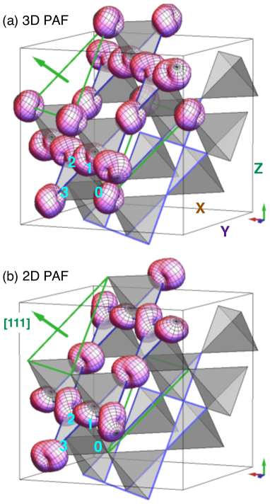
Figure 1: (a) 3D PAF [Eqs. (4) and (5)] and (b) 2D PAF [Eqs. (10) and (3)] electric quadrupole orders are schematically illustrated by deformation of the $f$-electron change density from that of the paramagnetic phase [26, 33].

The one-fold degeneracy of the mean-field PAF order with a wavevector $\bm{k}=(h,h,h)$ ($h>0$) is increased to three-fold in the limit of $h\rightarrow 0$. These three pseudospin LRO structures with $\bm{k}=0$ are expressed by (appendix)

$$\langle\bm{\sigma}_{\bm{t}_{n}+\bm{d}_{i}}\rangle\propto\bm{v}_{i}^{(j)}\;,$$ (4)

where $j=0,1,2$ with

$$\bm{v}_{i}^{(0)}=\begin{cases}\bm{y}_{i}&(i=1,2)\\ -\bm{y}_{i}&(i=0,3)\;,\end{cases}$$ (5)

$$\bm{v}_{i}^{(1)}=\begin{cases}\tfrac{\sqrt{3}}{2}\bm{x}_{i}-\tfrac{1}{2}\bm{y}_{i}&(i=1,3)\\ -\tfrac{\sqrt{3}}{2}\bm{x}_{i}+\tfrac{1}{2}\bm{y}_{i}&(i=0,2)\;,\end{cases}$$ (6)

and

$$\bm{v}_{i}^{(2)}=\begin{cases}\tfrac{\sqrt{3}}{2}\bm{x}_{i}+\tfrac{1}{2}\bm{y}_{i}&(i=0,1)\\ -\tfrac{\sqrt{3}}{2}\bm{x}_{i}-\tfrac{1}{2}\bm{y}_{i}&(i=2,3)\;.\end{cases}$$ (7)

Under zero field, these 3D PAF orders can be stabilized energetically or by an order-by-disorder mechanism [27], which will be shown by CMC simulations. Their order parameters may be decomposed into

$$m^{(j)}=\frac{\sum_{n,i}\bm{\sigma}_{\bm{t}_{n}+\bm{d}_{i}}\cdot\bm{v}_{i}^{(j)}}{\sum_{n,i}1}\;,$$ (8)

where the summation runs over all sites $\bm{t}_{n}+\bm{d}_{i}$. In the limit of $T\rightarrow 0$, $(\langle m^{(0)}\rangle,\langle m^{(1)}\rangle,\langle m^{(2)}\rangle)$ becomes $(\pm 1,0,0)$, $(0,\pm 1,0)$, or $(0,0,\pm 1)$. In CMC simulations we measure the average of

$$m_{\text{3DPAF}}=\sqrt{[m^{(0)}]^{2}+[m^{(1)}]^{2}+[m^{(2)}]^{2}}\;,$$ (9)

which represents the amplitude of the 3D PAF ordering.

In Fig. 1(a) we schematically illustrate the electric quadrupole order expressed by the pseudospin structure [Eqs. (4) and (5)]. We note that this “3D PAF” state is expressed by the “$T_{2g}$” state in Fig. 2(a) of Ref. [32], where a different notation is used: $J_{zz}=4J_{\text{nn,eff}}$, $J_{\pm}/J_{zz}=-\delta/2$, and $J_{\pm\pm}/J_{zz}=q/2$; the local $\bm{x}_{i}$ and $\bm{y}_{i}$ are rotated by 120 degrees from our definition.

III.2 Order parameter under [111] magnetic field

By taking a linear combination of Eq. (2) with various wavevectors $\bm{k}=(h,h,h)$ one can construct a 2D PAF pseudospin LRO which is non-zero only on an $\ell$-th kagomé lattice layer ($\ell=1,2,\cdots$)

$$\langle\bm{\sigma}_{\bm{t}_{n}+\bm{d}_{i}}\rangle\propto\bm{v}_{i}^{\text{2D}}\delta_{\ell,\hat{\bm{k}}\cdot(\bm{t}_{n}+\bm{d}_{i})}\;,$$ (10)

where $\hat{\bm{k}}$ is a vector parallel to the [111] direction such that $\hat{\bm{k}}\cdot(\bm{t}_{n}+\bm{d}_{i})=1,2,\cdots$ on the kagomé layers. In Fig. 1(b) we schematically illustrate the electric quadrupole order expressed by the pseudospin structure Eq. (10).

Since mean fields on the triangular layers ($i=0$ sites) vanish for the 2D PAF order, magnetic dipole moments on the triangular layers, $\langle\sigma_{\bm{t}_{n}+\bm{d}_{0}}^{z}\rangle\bm{z}_{0}$, can be easily induced by applying [111] magnetic field. When this magnetized state is stabilized against the 3D PAF state by low [111] magnetic fields, one can expect that the system behaves as a 2D PAF state on each kagomé layer, which is decoupled by field-induced ferromagnetic triangular layers.

Since $\bm{v}_{i}^{\text{2D}}$ [Eq. (3)] in Eq. (10) is expressed by $\bm{v}_{i}^{\text{2D}}=\tfrac{1}{2}\left[\bm{v}_{i}^{(0)}+\bm{v}_{i}^{(1)}+\bm{v}_{i}^{(2)}\right]$, we can define an order parameter of the 2D PAF order on a kagomé layer as

$$m_{\text{2DPAF}}=\tfrac{2}{3}\left(m^{(0)\prime}+m^{(1)\prime}+m^{(2)\prime}\right)$$ (11)

with

$$m^{(j)\prime}=\frac{\sum_{n,i}\bm{\sigma}_{\bm{t}_{n}+\bm{d}_{i}}\cdot\bm{v}_{i}^{(j)}}{\sum_{n,i}1}\;,$$ (12)

where the summation runs over sites on a single kagomé layer and an adjacent triangular layer. Under low [111] fields they become $\langle m^{(0)\prime}\rangle=\langle m^{(1)\prime}\rangle=\langle m^{(2)\prime}\rangle\simeq\pm\tfrac{1}{2}$ and $\langle m_{\text{2DPAF}}\rangle\simeq\pm 1$ at low temperatures. We will show that $m_{\text{2DPAF}}$ is the order parameter under low [111] fields by CMC simulations.

IV Results of CMC simulations

IV.1 Zero magnetic field

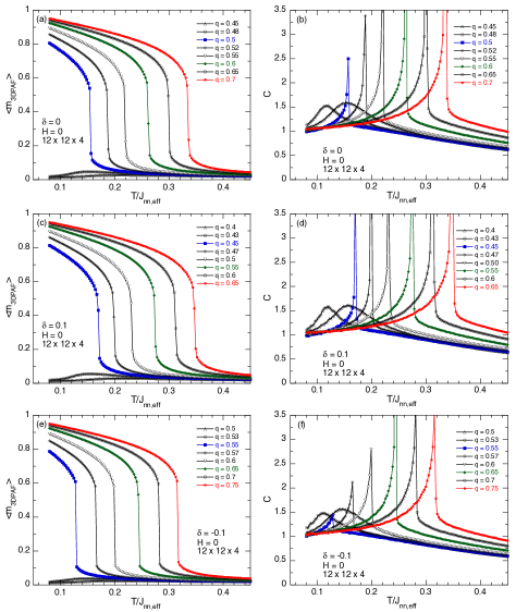
Figure 2: Temperature dependence of 3D PAF order parameter $\langle m_{\text{3DPAF}}\rangle$ and specific heat $C$ under zero field calculated by CMC simulations for various $q$ values. Shown in (a,b) are results with $\delta=0$; (c,d) and (e,f) are results with $\delta=0.1$, and $-0.1$, respectively.

Under zero magnetic field, it was shown that the classical ground state of the model for small $\delta$ changes from the classical spin ice state ($q<q_{\text{c}}=(1-\delta)/2$) to the PAF state ($q>q_{\text{c}}$) [27]. We performed CMC simulations using several parameter sets of the effective Hamiltonian to clarify whether the energetic or the order-by-disorder selection mechanism stabilizes the 3D PAF order. The simulations were performed with a lattice size of $L=12$ and $L^{\prime}=4$ ($12\times 12\times 4$). In Fig. 2 we plot the 3D-PAF order parameter $\langle m_{\text{3DPAF}}\rangle$ and the specific heat $C=(<E^{2}>-<E>^{2})/(NT^{2})$, where $E$ is the internal energy, as a function of temperature for $\delta=0,\pm 0.1$ and various $q$ values under zero field. One can see from Fig. 2(a) that $\langle m_{\text{3DPAF}}\rangle$ discontinuously increases below a critical temperature $T_{\text{c}}$ for $q\geq q_{\text{c}}$. This implies that the phase transition is first order and that the $\bm{k}=0$ order (3D PAF) occurs as expected. At the transition temperatures the specific heat [Fig. 2(b)] shows very sharp peaks. The CMC simulations with non-zero $\delta=0.1$ [Figs. 2(c) and (d)] and $\delta=-0.1$ [Figs. 2(e) and (f)] show parallel results with those of $\delta=0$. This confirms previous CMC simulations [26] and is consistent with a mean-field result (appendix) that small $\delta$ only changes $T_{\text{c}}$ [the largest eigenvalue Eq. (22)] as $T_{\text{c}}(q,\delta)=T_{\text{c}}(q,\delta=0)[1+\delta/(2q)]$, without affecting eigenvectors Eqs. (23) and (24).

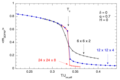
Figure 3: Size dependence of 3D PAF order parameter $\langle m_{\text{3DPAF}}\rangle$ as a function of temperature.

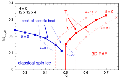
Figure 4: $T$-$q$ phase diagram determined by CMC simulations shown in Fig. 2. Red and blue thick lines are $T_{\text{c}}$ and broad peak of specific heat, respectively, obtained by simulations with $\delta=0$. Dashed and dotted thin lines are those with $\delta=\pm 0.1$.

Further CMC simulations with $(\delta,q)=(0,0.7)$ were performed to study size dependence of the 3D PAF order parameter. These results are shown in Fig. 3, which obviously demonstrates that the phase transition is first order. In Fig. 4 three curves of $T_{\text{c}}$ are plotted as a function of $q$ for $\delta=-0.1$, $0.0$, and $0.1$. It discontinuously decreases to $T_{\text{c}}=0$ at the critical value $q_{\text{c}}=-0.45$, $0.5$, and $0.55$ for $\delta=-0.1$, $0.0$, and $0.1$, respectively. This agrees with the first-order nature of the quantum phase transition, which was investigated by a quantum treatment [19]. In the range $q<q_{\text{c}}$ the specific heat shows only a broad peak at about $T/J_{\text{nn,eff}}\sim 0.2$, which can be interpreted as the behavior of the classical spin ice model [27]. We note that this peak temperature is significantly lower (about $1/4$) than that of the quantum MC simulation of the same model with parameters $q=0$ and $\delta\neq 0$ [43]. This implies that the temperature scale of the present CMC simulations is considerably reduced. Thereby one has to take account of this fact when comparing the CMC simulations with experimental data.

IV.2 Under [111] magnetic field

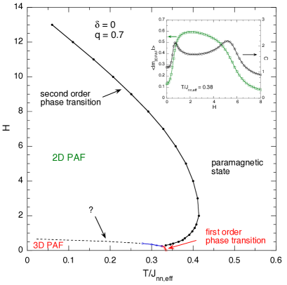
Figure 5: $H$-$T$ phase diagram under [111] magnetic field. There are the paramagnetic state and two LRO states of electric quadrupole moments denoted by 3D PAF and 2D PAF. Inset shows $H$ dependence of specific heat $C$ and 2D PAF order parameter $\langle|m_{\text{2DPAF}}|\rangle$ at $T/J_{\text{nn,eff}}=0.38$, which are calculated by simulations with lattice size $12\times 12\times 4$.

To study finite-temperature phase-transitions under [111] magnetic fields, we performed CMC simulations with a parameter set $(\delta,q)=(0,0.7)$ under various fields $H$. Figure 5 shows an approximate $H$-$T$ phase diagram obtained from peaks of the specific heat and jumps of the order parameter $\langle m_{\text{3DPAF}}\rangle$, which are calculated by simulations with lattice sizes $12\times 12\times 4$ and/or $6\times 6\times 2$. From the high-temperature paramagnetic phase the system undergoes a phase transition to one of the two quadrupole ordered phases denoted by 3D PAF and 2D PAF, which will be discussed later.

These 3D and 2D PAF phases are separated by a phase transition line, a crossover line, or multiple phase transitions (the dashed curve in Fig. 5). These three possibilities could not be clarified by the present simulation techniques, because the single-spin-flip simulations suffer from a freezing problem at low temperatures. We note that the boundary line between 3D PAF and 2D PAF states depicted by the dashed curve in Fig. 5 corresponds to the low-field kink of the $M$-$H$ curve shown in Fig. 5(b) of Ref. [26]. Simulated $M(H,T)$ data suggest that there may be intermediate magnetization plateau states between zero field and the low-field kink.

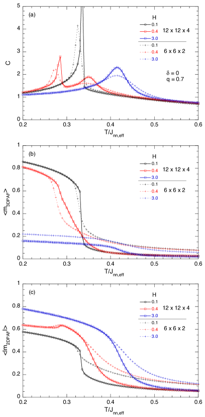
Figure 6: Temperature and size dependence of (a) specific heat $C$, (b) 3D PAF order parameter $\langle m_{\text{3DPAF}}\rangle$, and (c) 2D PAF order parameter $\langle|m_{\text{2DPAF}}|\rangle$ calculated by CMC simulations under three typical [111] fields $H=0.1$, 0.4, and 3.

Figure 6 shows temperature dependence of the specific heat $C$, the 3D-PAF order parameter $\langle m_{\text{3DPAF}}\rangle$, and the 2D-PAF order parameter $\langle|m_{\text{2DPAF}}|\rangle$ under three typical magnetic fields: $H=0.1$, 0.4, and 3. At the low field $H=0.1$ it is evident that the system shows the same first-order phase transition as zero field, and that LRO is the 3D PAF order. On the other hand, at the high field $H=3$, the size dependence of $C(T)$ and $\langle|m_{\text{2DPAF}}|\rangle(T)$ [Figs. 6(a) and 6(c)] show typical behaviors of a second-order phase-transition. These indicate that $\langle|m_{\text{2DPAF}}|\rangle$ is the order parameter of the second-order phase-transition, in agreement with the initial expectation. At the intermediate field $H=0.4$ the temperature dependence of the specific heat [Fig. 6(a)] implies that two successive phase transitions occur. At the higher $T_{\text{c}1}/J_{\text{nn,eff}}\simeq 0.35$, $C(T)$ and $\langle|m_{\text{2DPAF}}|\rangle(T)$ [Figs. 6(a) and 6(c)] show that the phase transition is the same kind as that for $H=3$. On the other hand, characteristics of the lower $T_{\text{c}2}/J_{\text{nn,eff}}\simeq 0.28$ are less clear owing to the freezing problem. The simulated $C(T)$, $\langle m_{\text{3DPAF}}\rangle(T)$, and $\langle|m_{\text{2DPAF}}|\rangle(T)$ (Fig. 6) suggest that $T_{\text{c}2}$ is a continuous phase transition between 2D PAF and 3D PAF states, which could not be further investigated using the present techniques. In addition to the constant $H$ plots (Fig. 6), magnetic field dependence of $C$ and $\langle|m_{\text{2DPAF}}|\rangle$ with constant $T=0.38J_{\text{nn,eff}}$ are shown in the inset of Fig. 5. At this temperature reentrant phase transitions occur at lower and upper critical fields, $H_{\text{c1}}\simeq 0.7$ and $H_{\text{c2}}\simeq 5.2$.

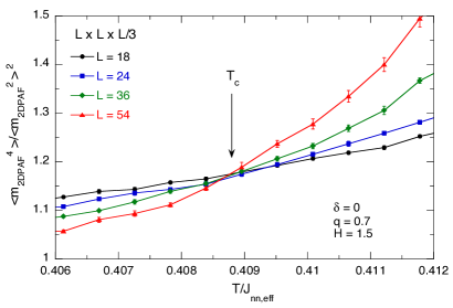
Figure 7: Temperature dependence of the Binder cumulant $\left<m_{\text{2DPAF}}^{4}\right>/\left<m_{\text{2DPAF}}^{2}\right>^{2}$ close to $T_{\text{c}}$ for lattice sizes $L=18,24,36$, and $54$ under [111] field $H=1.5$.

Since the 2D PAF order breaks a $Z_{2}$ symmetry of $m_{\text{2DPAF}}$, one can naturally expect that its second-order phase-transition at $T_{\text{c}}$ belongs to the universality class of the 2D Ising model. To confirm this universality we performed standard finite-size scaling analyses [36] on CMC simulation data taken under a typical [111] field $H=1.5$. These simulations were carried out on clusters with lattice sizes $L\times L\times(L/3)$ with $L=18,24,36$, and $54$. Figure 7 shows the Binder cumulant $U_{4}=\left<m_{\text{2DPAF}}^{4}\right>/\left<m_{\text{2DPAF}}^{2}\right>^{2}$ as a function of temperature. These curves with different lattice sizes cross at a single point, which enables us to determine the critical temperature $T_{\text{c}}/J_{\text{nn,eff}}=0.4088(2)$.

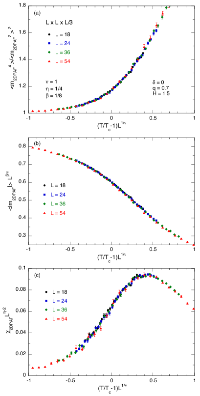
Figure 8: Finite size scaling of (a) the Binder cumulant $\left<m_{\text{2DPAF}}^{4}\right>/\left<m_{\text{2DPAF}}^{2}\right>^{2}$, (b) 2D PAF order parameter $\langle|m_{\text{2DPAF}}|\rangle$, and (c) 2D PAF susceptibility $\chi_{\text{2DPAF}}$.

The theory of the finite-size scaling indicates that the Binder cumulant, the order parameter $\left<|m_{\text{2DPAF}}|\right>$, and the susceptibility $\chi_{\text{2DPAF}}=N_{\text{2D}}\left(\left<m_{\text{2DPAF}}^{2}\right>-\left<|m_{\text{2DPAF}}|\right>^{2}\right)/T$ show the scaling forms

$$U_{4} =f(L^{1/\nu}(T-T_{\text{c}})/T_{\text{c}})\;,$$

$$\left<|m_{\text{2DPAF}}|\right> =L^{-\beta/\nu}g(L^{1/\nu}(T-T_{\text{c}})/T_{\text{c}})\;,$$ (13)

$$\chi_{\text{2DPAF}} =L^{2-\eta}h(L^{1/\nu}(T-T_{\text{c}})/T_{\text{c}})\;,$$

where $f$, $g$, and $h$ are universal functions [36]. In Fig. 8 we show these finite-size scaling plots using the exact critical exponents $\nu=1$, $\beta=1/8$, and $\eta=1/4$ for the 2D Ising model. These figures show excellent data collapse, which proves the finite-size scaling relations of the 2D Ising model. Therefore we conclude that the second-order phase-transition of the 2D PAF state belongs to the 2D Ising universality class.

To complement the argument of the 2D Ising universality class we calculated squares of the Fourier transform of $m_{\text{2DPAF}}$ [Eq. (11)], which is defined on each $\ell$-th kagomé lattice layer, with wavevectors $\bm{k}=(h,h,h)$ ($0\leq h\leq 1$)

$$|m_{\text{2DPAF}}(\bm{k})|^{2}=\left|\sum_{\ell}\left[m_{\text{2DPAF}}\right]_{\ell}\,e^{i\bm{k}\cdot\bm{r}}\right|^{2},$$ (14)

where $\bm{r}$ is a lattice position on the $\ell$-th kagomé lattice layer. If $m_{\text{2DPAF}}$ has really 2D character, simulated averages of $|m_{\text{2DPAF}}(\bm{k})|^{2}$ do not depend on $h$. In terms of a scattering experiment (assuming that the quadrupole moment would be visible), $\langle|m_{\text{2DPAF}}(\bm{k})|^{2}\rangle$ is constant between two $\Gamma$ points $\bm{k}=(0,0,0)$ and $(1,1,1)$. In Fig. 9 we show CMC averages $\langle|m_{\text{2DPAF}}(\bm{k})|^{2}\rangle$ close to $T_{\text{c}}$, which were computed with a lattice size $12\times 12\times 4$. These curves show independence of $h$ and thereby the two dimensionality of the order parameter. We note that the freezing problem of the present CMC techniques prohibited us from performing simulations with larger system sizes and from obtaining the averages at low temperatures ($T\ll T_{\text{c}}$). This difficulty is seen as the large error estimation of the low-temperature data ($T\leq T_{\text{c}}$) shown in Fig. 9. Despite this large error, we also note that one may see slight wavevector dependence for the curve at $T=0.40J_{\text{nn,eff}}<T_{\text{c}}$. This may suggest that the 2D PAF order is weakly modulated along the [111] direction at low temperatures.

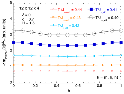
Figure 9: Wavevector dependence of $\langle|m_{\text{2DPAF}}(\bm{k})|\rangle^{2}$ along [111] direction above and below $T_{\text{c}}$ computed by CMC simulations with lattice size $12\times 12\times 4$. Size of symbol represents estimated error of data.

V Discussion

In previous investigations [26, 28] we showed that the simple pseudospin-$\frac{1}{2}$ Hamiltonian described by Eq. (1) qualitatively and semi-quantitatively accounts for most of the experimental observations of the TTO sample with $T_{\text{c}}>0$ by selecting the appropriate model parameters. The agreement between experiments and theories was surprisingly better than our initial expectation. This means that the model Hamiltonian essentially explains the experimentally observed properties of TTO. Although there remain problems of oversimplifications caused by the classical approximations for the quantum model and by neglecting effects of higher-energy CF states [32] and Jahn-Teller effects due to the phonon mechanism [44].

We would like to make a few comments on the the present CMC simulation results in relation to experimental observations. A first comment is on the natural question: how does the off-stoichiometry parameter of Tb_2+xTi_2-xO_7+y, $x$ (and/or $y$), function as the tuning parameter between QSL and quadrupolar states? Our experiments using both poly- and single-crystalline samples showed that $x_{\text{c}}\simeq-0.0025$ is the quantum critical point [24, 25]. They also showed that by approaching to $x_{\text{c}}$ from the quadrupolar side $x>x_{\text{c}}$, the large specific-heat peak observed in $C(T)$ data (e.g. Fig. 4(a) in Ref. [26]) abruptly becomes smaller peaks as shown in Fig. 2 of Ref. [24] and Fig. 4(a) of Ref. [25]. By assuming that the change of $x$ is equivalent to that of $q$, the experimental behavior of $C(T)$ is approximately reproduced by the simulated $C(T)$ shown in Fig. 2(b). Therefore an answer to the question may be that $x$ tunes the ratio of the magnitude of the quadrupole interaction to that of the magnetic interaction.

A second comment is on susceptibilities under zero field. We calculated the magnetic susceptibility $\chi_{\parallel[111]}=N\left(\langle m_{\parallel[111]}^{2}\rangle-\langle|m_{\parallel[111]}|\rangle^{2}\right)/T$ using the same parameter sets as those of Fig. 2(a). These results are shown in Fig. 10(a). The curve with $q=0.55$ bears resemblance to the experimental data of the TTO sample with $T_{\text{c}}=0.53$ K (Fig. 2(a) of Ref. [26]). If we take account of the reduction of the temperature scale for the CMC simulation the resemblance becomes more striking. This also can justify the interpretation of TTO using the model Hamiltonian and the CMC simulation. We also calculated the electric quadrupole susceptibility corresponding to the 3D PAF order $\chi_{m_{\text{3DPAF}}}=N\left(\langle m_{\text{3DPAF}}^{2}\rangle-\langle|m_{\text{3DPAF}}|\rangle^{2}\right)/T$. Temperature dependence of this quadrupole susceptibility is shown in Fig. 10(b). The large increase of $\chi_{m_{\text{3DPAF}}}$ close to $T_{\text{c}}$ can be measured by ultrasonic experiments of TTO, for example, extending measurements of Ref. [45] down to 0.3 K.

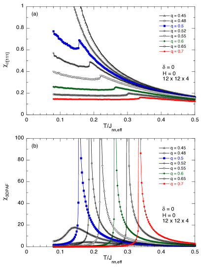
Figure 10: Temperature dependence of (a) magnetic susceptibility parallel to [111] direction $\chi_{\parallel[111]}$ and (b) susceptibility of $m_{\text{3DPAF}}$ under zero field calculated by CMC simulations.

A third comment is on the first-order nature of the zero-field phase-transition of the CMC simulations. This does not agree with experimental $C(T)$, which shows a second-order behavior [26]. In addition, the second-order phase-transition under [111] field seems to be somewhat smeared out for the the experimental data (Fig. 4(a,b) of Ref. [26]) compared to the CMC simulations. These disagreements remain to be explained, e.g., by adding a higher-order term in the Hamiltonian [46], by a disorder effect [47], or possibly by a quantum effect.

VI Conclusions

We have studied phase transitions of pyrochlore magnets with non-Kramers ions under [111] magnetic field represented by the effective pseudospin-$\frac{1}{2}$ Hamiltonian [27] from a viewpoint of relevance to electric quadrupolar states of Tb₂Ti₂O₇ [26]. Order parameters and finite-temperature phase-transitions of this frustrated model system are investigated using classical Monte-Carlo simulations. In zero field, the model undergoes a first-order phase-transition from the paramagnetic state to a 3D quadrupolar state with an antiparallel arrangement of pseudospins. This 3D order is selected energetically or by an order-by-disorder mechanism from degenerate $\bm{k}=(h,h,h)$ mean-field orders. Under [111] magnetic field this 3D state is transformed to a 2D quadrupolar state on each kagomé lattice, which is separated by field-induced ferromagnetic triangular lattices. This 2D system undergoes a second-order phase-transition belonging to the 2D Ising universality class.

*

Appendix A Definitions of Hamiltonian and classical mean-field theory

Detailed definitions of the Hamiltonian and pseudospin orders within a classical mean-field theory are summarized in this section. The CF ground state doublet of TTO [33] can be written by

$$|\pm 1\rangle_{\text{D}}=A|\mp 4\rangle\pm B|\mp 1\rangle+C|\pm 2\rangle\mp D|\pm 5\rangle\;,$$ (15)

where $|m\rangle$ stands for the $|J=6,m\rangle$ state within a $JLS$-multiplet [48]. Using CF parameters of Ref. [49] the coefficients of Eq. (15) are $A=0.9581$, $B=0.1284$, $C=0.1210$, $D=0.2256$. Magnetic-dipole and electric-quadrupole moment operators [50] within $|\pm 1\rangle_{\text{D}}$ are proportional to the Pauli matrices $\sigma^{\alpha}$ ($\alpha=x,y,z$) and the unit matrix [33]: magnetic moment operators

$$J_{x} =J_{y}=0,$$

$$J_{z} =-(4A^{2}+B^{2}-2C^{2}-5D^{2})\sigma^{z}\;,$$ (16)

and quadrupole moment operators

$$\tfrac{1}{2}[3J_{z}^{2}-J(J+1)] =3A^{2}-\tfrac{39}{2}B^{2}-15C^{2}+\tfrac{33}{2}D^{2},$$

$$\tfrac{\sqrt{3}}{2}[J_{x}^{2}-J_{y}^{2}] =\left(-\tfrac{21\sqrt{3}}{2}B^{2}+9\sqrt{10}AC\right)\sigma^{x},$$

$$\tfrac{\sqrt{3}}{2}[J_{x}J_{y}+J_{y}J_{x}] =-\left(-\tfrac{21\sqrt{3}}{2}B^{2}+9\sqrt{10}AC\right)\sigma^{y},$$

$$\tfrac{\sqrt{3}}{2}[J_{z}J_{x}+J_{x}J_{z}] =-\left(3\sqrt{30}BC+9\sqrt{\tfrac{33}{2}}AD\right)\sigma^{x},$$

$$\tfrac{\sqrt{3}}{2}[J_{y}J_{z}+J_{z}J_{y}] =-\left(3\sqrt{30}BC+9\sqrt{\tfrac{33}{2}}AD\right)\sigma^{y}\;.$$ (17)

The operators $\sigma_{\bm{r}}^{\alpha}$ of Eq. (1) act on $|\pm 1\rangle_{\text{D}}$ at each pyrochlore lattice site $\bm{r}=\bm{t}_{n}+\bm{d}_{i}$, where $\bm{t}_{n}$ is an FCC translation vector and $\bm{d}_{i}$ ($i=0,1,2,3$) are four crystallographic sites in the unit cell. Coordinates of these sites $\bm{d}_{i}$ and their local axes $\bm{x}_{i}$, $\bm{y}_{i}$, and $\bm{z}_{i}$ are listed in Table 1. The phases $\phi_{\bm{r},\bm{r}^{\prime}}$ of Eq. (1) are $\phi_{\bm{t}_{n}+\bm{d}_{i},\bm{t}_{n^{\prime}}+\bm{d}_{i^{\prime}}}=0$, $-2\pi/3$, and $2\pi/3$ for site pairs of $(i,i^{\prime})=(0,3),(1,2)$, $(i,i^{\prime})=(0,1),(2,3)$, and $(i,i^{\prime})=(0,2),(1,3)$, respectively, where the notation of Ref. [27] is used.

Table 1: Coordinates of four crystallographic sites $\bm{d}_{i}$ and their local axes $\bm{x}_{i}$, $\bm{y}_{i}$, and $\bm{z}_{i}$ [33]. These coordinates are defined using (global) cubic XYZ axes shown in Fig. 1(a). The four sites $\bm{d}_{i}$ are illustrated by vertices with light blue numbers ($i=0,1,2,3$) of a tetrahedron in Fig. 1(a).

$i$	$\bm{d}_{i}$	$\bm{x}_{i}$	$\bm{y}_{i}$	$\bm{z}_{i}$
0	$\tfrac{1}{4}(0,0,0)$	$\tfrac{1}{\sqrt{6}}(1,1,-2)$	$\tfrac{1}{\sqrt{2}}(-1,1,0)$	$\tfrac{1}{\sqrt{3}}(1,1,1)$
1	$\tfrac{1}{4}(0,1,1)$	$\tfrac{1}{\sqrt{6}}(1,-1,2)$	$\tfrac{1}{\sqrt{2}}(-1,-1,0)$	$\tfrac{1}{\sqrt{3}}(1,-1,-1)$
2	$\tfrac{1}{4}(1,0,1)$	$\tfrac{1}{\sqrt{6}}(-1,1,2)$	$\tfrac{1}{\sqrt{2}}(1,1,0)$	$\tfrac{1}{\sqrt{3}}(-1,1,-1)$
3	$\tfrac{1}{4}(1,1,0)$	$\tfrac{1}{\sqrt{6}}(-1,-1,-2)$	$\tfrac{1}{\sqrt{2}}(1,-1,0)$	$\tfrac{1}{\sqrt{3}}(-1,-1,1)$

Possible pseudospin LROs of Eq. (1) under zero magnetic field were discussed in Ref. [27]. We summarize a few results of the classical mean-field theory [27] to facilitate gaining insight of order parameters for the PAF phase (Fig. 7 in Ref. [27]; $q>q_{\text{c}}$). The effective Hamiltonian of Eq. (1) under zero magnetic field can be expressed using the Fourier transform as

$$\mathcal{H}\propto-J_{\text{nn,eff}}\sum_{\bm{k},i,i^{\prime},\alpha,\beta}\sigma_{\bm{k},i}^{\alpha}J_{i,\alpha;i^{\prime},\beta}(\bm{k})\sigma_{\bm{k},i^{\prime}}^{\beta}\;,$$ (18)

where the summation runs over wavevectors $\bm{k}$ in the first Brillouin zone, $i,i^{\prime}=0,1,2,3$ and $\alpha,\beta=x,y,z$, and $\sigma_{\bm{t}_{n}+\bm{d}_{i}}^{\alpha}=\sum_{\bm{k}}\sigma_{\bm{k},i}^{\alpha}e^{i\bm{k}\cdot(\bm{t}_{n}+\bm{d}_{i})}$. The matrix $J_{i,\alpha;i^{\prime},\beta}(\bm{k})$ stands for the Fourier transform of the superexchange coupling constants $J_{n,i,\alpha;n^{\prime},i^{\prime},\beta}$ between $\sigma_{\bm{t}_{n}+\bm{d}_{i}}^{\alpha}$ and $\sigma_{\bm{t}_{n^{\prime}}+\bm{d}_{i^{\prime}}}^{\beta}$:

$$J_{i,\alpha;i^{\prime},\beta}(\bm{k})=\sum_{n}J_{n,i,\alpha;n^{\prime},i^{\prime},\beta}e^{i\bm{k}\cdot[(\bm{t}_{n}+\bm{d}_{i})-(\bm{t}_{n^{\prime}}+\bm{d}_{i^{\prime}})]}\;.$$ (19)

The critical temperature $T_{\text{c}}$ and pseudospin LRO are obtained by the largest eigenvalue ($\propto T_{\text{c}}$) and corresponding eigenvectors of $J_{i,\alpha;i^{\prime},\beta}(\bm{k})$.

The largest eigenvalue of $J_{i,\alpha;i^{\prime},\beta}(\bm{k})$ is degenerate on four symmetry-equivalent lines $\bm{k}=(h,\pm h,h)$ and $(h,h,\pm h)$, where $|h|\leq\tfrac{1}{2}$ [27]. On a degeneracy line $\bm{k}=(h,h,h)$, the $12\times 12$ matrix $J_{i,\alpha;i^{\prime},\beta}(\bm{k})$ consists of magnetic $4\times 4$ and quadrupolar $8\times 8$ blocks: the magnetic submatrix

$$J_{i,z;i^{\prime},z}(\bm{k}=(h,h,h))=-J_{\text{nn,eff}}$$

$$\times\begin{pmatrix}0&\cos(\pi h)&\cos(\pi h)&\cos(\pi h)\\ \cos(\pi h)&0&1&1\\ \cos(\pi h)&1&0&1\\ \cos(\pi h)&1&1&0\\ \end{pmatrix}\;,$$ (20)

which acts on a vector $(\sigma_{\bm{k},0}^{z},\sigma_{\bm{k},1}^{z},\sigma_{\bm{k},2}^{z},\sigma_{\bm{k},2}^{z})^{\text{T}}$, and the quadrupolar submatrix

$$J_{i,\alpha;i^{\prime},\beta}(\bm{k}=(h,h,h))=-J_{\text{nn,eff}}$$

$$\times\begin{pmatrix}0&\cos(\pi h)M_{1}&\cos(\pi h)M_{2}&\cos(\pi h)M_{3}\\ \cos(\pi h)M_{1}&0&M_{3}&M_{2}\\ \cos(\pi h)M_{2}&M_{3}&0&M_{1}\\ \cos(\pi h)M_{3}&M_{2}&M_{1}&0\\ \end{pmatrix}\;,$$ (21)

which acts on a vector $(\sigma_{\bm{k},0}^{x},\sigma_{\bm{k},0}^{y},\sigma_{\bm{k},1}^{x},\sigma_{\bm{k},1}^{y},\sigma_{\bm{k},2}^{x},\sigma_{\bm{k},2}^{y},\sigma_{\bm{k},3}^{x},\sigma_{\bm{k},3}^{y})^{\text{T}}$. In Eq. (21) $M_{i}$ ($i=1,2,3$) stand for $2\times 2$ matrices $M_{1}=\begin{pmatrix}\delta-\tfrac{1}{2}q&-\tfrac{\sqrt{3}}{2}q\\ -\tfrac{\sqrt{3}}{2}q&\delta+\tfrac{1}{2}q\\ \end{pmatrix}$   , $M_{2}=\begin{pmatrix}\delta-\tfrac{1}{2}q&\tfrac{\sqrt{3}}{2}q\\ \tfrac{\sqrt{3}}{2}q&\delta+\tfrac{1}{2}q\\ \end{pmatrix}$   , and $M_{3}=\begin{pmatrix}\delta+q&0\\ 0&\delta-q\\ \end{pmatrix}$. One can show that the largest eigenvalue of $J_{i,\alpha;i^{\prime},\beta}(\bm{k})$ is that of Eq. (21), which is exactly

$$J_{\text{nn,eff}}(2q+\delta)$$ (22)

for small $\delta$ (PAF phase).

One can also show that the degeneracy of the largest eigenvalue is one and three fold for $|h|>0$ and $h=0$, respectively, and that the corresponding eigenvectors, which depend on neither $q$ nor $\delta$, are given by

$$\begin{pmatrix}\sigma_{\bm{k},0}^{x}\\ \sigma_{\bm{k},0}^{y}\\ \sigma_{\bm{k},1}^{x}\\ \sigma_{\bm{k},1}^{y}\\ \sigma_{\bm{k},2}^{x}\\ \sigma_{\bm{k},2}^{y}\\ \sigma_{\bm{k},3}^{x}\\ \sigma_{\bm{k},3}^{y}\\ \end{pmatrix}=\begin{pmatrix}0\\ 0\\ \tfrac{\sqrt{3}}{2}\\ \tfrac{1}{2}\\ -\tfrac{\sqrt{3}}{2}\\ \tfrac{1}{2}\\ 0\\ -1\\ \end{pmatrix}$$ (23)

[Eq. (3)] for $|h|>0$ and by

$$\begin{pmatrix}\sigma_{\bm{0},0}^{x}\\ \sigma_{\bm{0},0}^{y}\\ \sigma_{\bm{0},1}^{x}\\ \sigma_{\bm{0},1}^{y}\\ \sigma_{\bm{0},2}^{x}\\ \sigma_{\bm{0},2}^{y}\\ \sigma_{\bm{0},3}^{x}\\ \sigma_{\bm{0},3}^{y}\\ \end{pmatrix}=\begin{pmatrix}0\\ -1\\ 0\\ 1\\ 0\\ 1\\ 0\\ -1\\ \end{pmatrix}\,,\begin{pmatrix}-\tfrac{\sqrt{3}}{2}\\ \tfrac{1}{2}\\ \tfrac{\sqrt{3}}{2}\\ -\tfrac{1}{2}\\ -\tfrac{\sqrt{3}}{2}\\ \tfrac{1}{2}\\ \tfrac{\sqrt{3}}{2}\\ -\tfrac{1}{2}\\ \end{pmatrix}\,,\begin{pmatrix}\tfrac{\sqrt{3}}{2}\\ \tfrac{1}{2}\\ \tfrac{\sqrt{3}}{2}\\ \tfrac{1}{2}\\ -\tfrac{\sqrt{3}}{2}\\ -\tfrac{1}{2}\\ -\tfrac{\sqrt{3}}{2}\\ -\tfrac{1}{2}\\ \end{pmatrix}$$ (24)

[Eqs. (5), (6), (7)] for $h=0$. Therefore, it is very likely that pseudospin LROs of Eq. (1) just below $T_{\text{c}}$ under zero magnetic field are either the mean-field PAF order [Eq. (23)] or the 3D PAF order [Eq. (24)]. Although it is not obvious which PAF order is selected, one can expect that at sufficiently low temperatures an energetic or an order-by-disorder mechanism stabilizes the 3D PAF order. We note that for the PAF order [Eq. (23)] the mean field at the triangular lattice site ($\bm{d}_{i=0}$) vanishes, which implies that the PAF order is essentially 2D LRO on each kagomé lattice layer.

References

- Lacroix et al. [2011] C. Lacroix, P. Mendels, and F. Mila, eds., Introduction to Frustrated Magnetism (Springer, Berlin, Heidelberg, 2011).
- Wannier [1950] G. H. Wannier, Antiferromagnetism. the triangular ising net, Phys. Rev. 79, 357 (1950).
- Syôzi [1951] I. Syôzi, Prog. Theor. Phys. , 306 (1951).
- Qi et al. [2008] Y. Qi, T. Brintlinger, and J. Cumings, Direct observation of the ice rule in an artificial kagome spin ice, Phys. Rev. B 77, 094418 (2008).
- Gardner et al. [2010] J. S. Gardner, M. J. P. Gingras, and J. E. Greedan, Magnetic pyrochlore oxides, Rev. Mod. Phys. 82, 53 (2010).
- Bramwell and Gingras [2001] S. T. Bramwell and M. J. P. Gingras, Science 294, 1495 (2001).
- Ramirez et al. [1999] A. P. Ramirez, A. Hayashi, R. J. Cava, R. Siddharthan, and B. S. Shastry, Zero-point entropy in ‘spin ice’, Nature (London) 399, 333 (1999).
- Matsuhira et al. [2002] K. Matsuhira, Z. Hiroi, T. Tayama, S. Takagi, and T. Sakakibara, LETTER TO THE EDITOR: A new macroscopically degenerate ground state in the spin ice compound Dy2Ti2O7 under a magnetic field, J. Phys. Condens. Matter 14, L559 (2002).
- Tabata et al. [2006] Y. Tabata, H. Kadowaki, K. Matsuhira, Z. Hiroi, N. Aso, E. Ressouche, and B. Fåk, Kagomé Ice State in the Dipolar Spin Ice , Phys. Rev. Lett. 97, 257205 (2006).
- Fennell et al. [2007] T. Fennell, S. T. Bramwell, D. F. McMorrow, P. Manuel, and A. R. Wildes, Pinch points and Kasteleyn transitions in kagome ice, Nature Physics 3, 566 (2007).
- Castelnovo et al. [2008] C. Castelnovo, R. Moessner, and S. L. Sondhi, Magnetic monopoles in spin ice, Nature 451, 42 (2008).
- Kadowaki et al. [2009] H. Kadowaki, N. Doi, Y. Aoki, Y. Tabata, T. J. Sato, J. W. Lynn, K. Matsuhira, and Z. Hiroi, Observation of Magnetic Monopoles in Spin Ice, J. Phys. Soc. Jpn. 78, 103706 (2009).
- Jaubert et al. [2013] L. D. C. Jaubert, M. J. Harris, T. Fennell, R. G. Melko, S. T. Bramwell, and P. C. W. Holdsworth, Topological-sector fluctuations and curie-law crossover in spin ice, Phys. Rev. X 3, 011014 (2013).
- Lee [2008] P. A. Lee, An end to the drought of quantum spin liquids, Science 321, 1306 (2008).
- Balents [2010] L. Balents, Spin liquids in frustrated magnets, Nature (London) 464, 199 (2010).
- Savary and Balents [2017] L. Savary and L. Balents, Quantum spin liquids: a review, Rep. Prog. Phys. 80, 016502 (2017).
- Hermele et al. [2004] M. Hermele, M. P. A. Fisher, and L. Balents, Pyrochlore photons: The spin liquid in a three-dimensional frustrated magnet, Phys. Rev. B 69, 064404 (2004).
- Benton et al. [2012] O. Benton, O. Sikora, and N. Shannon, Seeing the light: Experimental signatures of emergent electromagnetism in a quantum spin ice, Phys. Rev. B 86, 075154 (2012).
- Lee et al. [2012] S. Lee, S. Onoda, and L. Balents, Generic quantum spin ice, Phys. Rev. B 86, 104412 (2012).
- Gingras and McClarty [2014] M. J. P. Gingras and P. A. McClarty, Quantum spin ice: a search for gapless quantum spin liquids in pyrochlore magnets, Rep. Prog. Phys. 77, 056501 (2014).
- Gardner et al. [1999] J. S. Gardner, S. R. Dunsiger, B. D. Gaulin, M. J. P. Gingras, J. E. Greedan, R. F. Kiefl, M. D. Lumsden, W. A. MacFarlane, N. P. Raju, J. E. Sonier, I. Swainson, and Z. Tun, Cooperative Paramagnetism in the Geometrically Frustrated Pyrochlore Antiferromagnet , Phys. Rev. Lett. 82, 1012 (1999).
- Kadowaki et al. [2018] H. Kadowaki, M. Wakita, B. Fåk, J. Ollivier, S. Ohira-Kawamura, K. Nakajima, H. Takatsu, and M. Tamai, Continuum Excitation and Pseudospin Wave in Quantum Spin-Liquid and Quadrupole Ordered States of Tb2+xTi2-xO7+y, J. Phys. Soc. Jpn. 87, 064704 (2018).
- Molavian et al. [2007] H. R. Molavian, M. J. P. Gingras, and B. Canals, Dynamically Induced Frustration as a Route to a Quantum Spin Ice State in Tb2Ti2O7 via Virtual Crystal Field Excitations and Quantum Many-Body Effects, Phys. Rev. Lett. 98, 157204 (2007).
- Taniguchi et al. [2013] T. Taniguchi, H. Kadowaki, H. Takatsu, B. Fåk, J. Ollivier, T. Yamazaki, T. J. Sato, H. Yoshizawa, Y. Shimura, T. Sakakibara, T. Hong, K. Goto, L. R. Yaraskavitch, and J. B. Kycia, Long-range order and spin-liquid states of polycrystalline Tb2+xTi2-xO7+y, Phys. Rev. B 87, 060408 (2013).
- Wakita et al. [2016] M. Wakita, T. Taniguchi, H. Edamoto, H. Takatsu, and H. Kadowaki, Quantum spin liquid and electric quadrupolar states of single crystal Tb2+xTi2-xO7+y, J. Phys.: Conf. Series 683, 012023 (2016).
- Takatsu et al. [2016a] H. Takatsu, S. Onoda, S. Kittaka, A. Kasahara, Y. Kono, T. Sakakibara, Y. Kato, B. Fåk, J. Ollivier, J. W. Lynn, T. Taniguchi, M. Wakita, and H. Kadowaki, Quadrupole Order in the Frustrated Pyrochlore , Phys. Rev. Lett. 116, 217201 (2016a).
- Onoda and Tanaka [2011] S. Onoda and Y. Tanaka, Quantum fluctuations in the effective pseudospin- model for magnetic pyrochlore oxides, Phys. Rev. B 83, 094411 (2011).
- Takatsu et al. [2016b] H. Takatsu, T. Taniguchi, S. Kittaka, T. Sakakibara, and H. Kadowaki, Quadrupole order in the frustrated pyrochlore magnet Tb2Ti2O7, J. Phys.: Conf. Series 683, 012022 (2016b).
- Takatsu et al. [2017] H. Takatsu, T. Taniguchi, S. Kittaka, T. Sakakibara, and H. Kadowaki, Thermodynamic properties of quadrupolar states in the frustrated pyrochlore magnet Tb2Ti2O7, J. Phys.: Conf. Series 828, 012007 (2017).
- Bojesen and Onoda [2017] T. A. Bojesen and S. Onoda, Quantum spin ice under a [111] magnetic field: From pyrochlore to kagome, Phys. Rev. Lett. 119, 227204 (2017).
- Zhitomirsky et al. [2014] M. E. Zhitomirsky, P. C. W. Holdsworth, and R. Moessner, Nature of finite-temperature transition in anisotropic pyrochlore , Phys. Rev. B 89, 140403 (2014).
- [32] J. G. Rau and M. J. P. Gingras, arXiv:1806.09638.
- Kadowaki et al. [2015] H. Kadowaki, H. Takatsu, T. Taniguchi, B. Fåk, and J. Ollivier, Composite Spin and Quadrupole Wave in the Ordered Phase of Tb2+xTi2-xO7+y, SPIN 05, 1540003 (2015).
- den Hertog and Gingras [2000] B. C. den Hertog and M. J. P. Gingras, Dipolar interactions and origin of spin ice in ising pyrochlore magnets, Phys. Rev. Lett. 84, 3430 (2000).
- [35] The parameter values of , , and in this paper are obtained by converting the typical parameters K, K, , and of Ref. [26] using the relation , by which the dipolar interaction can be effectively included [34].
- Landau and Binder [2015] D. P. Landau and K. Binder, A Guide to Monte Carlo Simulations in Statistical Physics (Cambridge University Press, Cambridge, Heidelberg, 2015).
- Sachdev [2011] S. Sachdev, Quantum Phase Transitions (Cambridge University Press, Cambridge, New York, 2011).
- Hukushima and Nemoto [1996] K. Hukushima and K. Nemoto, Exchange monte carlo method and application to spin glass simulations, J. Phys. Soc. Jpn. 65, 1604 (1996).
- [39] H. Kadowaki, https://github.com/kadowaki-h/MCsimulationQOpyrochlore.
- Bauer et al. [2011] B. Bauer, L. D. Carr, H. G. Evertz, A. Feiguin, J. Freire, S. Fuchs, L. Gamper, J. Gukelberger, E. Gull, S. Guertler, A. Hehn, R. Igarashi, S. V. Isakov, D. Koop, P. N. Ma, P. Mates, H. Matsuo, O. Parcollet, G. Pawłowski, J. D. Picon, L. Pollet, E. Santos, V. W. Scarola, U. Schollwöck, C. Silva, B. Surer, S. Todo, S. Trebst, M. Troyer, M. L. Wall, P. Werner, and S. Wessel, The alps project release 2.0: open source software for strongly correlated systems, J. Stat. Mech. 2011, P05001 (2011).
- Albuquerque et al. [2007] A. F. Albuquerque, F. Alet, P. Corboz, P. Dayal, A. Feiguin, S. Fuchs, L. Gamper, E. Gull, S. Gürtler, A. Honecker, R. Igarashi, M. Körner, A. Kozhevnikov, A. Läuchli, S. R. Manmana, M. Matsumoto, I. P. McCulloch, F. Michel, R. M. Noack, G. Pawłowski, L. Pollet, T. Pruschke, U. Schollwöck, S. Todo, S. Trebst, M. Troyer, P. Werner, S. Wessel, and the ALPS Collaboration, The ALPS project release 1.3: Open-source software for strongly correlated systems, Journal of Magnetism and Magnetic Materials 310, 1187 (2007).
- Palmer and Chalker [2000] S. E. Palmer and J. T. Chalker, Order induced by dipolar interactions in a geometrically frustrated antiferromagnet, Phys. Rev. B 62, 488 (2000).
- Kato and Onoda [2015] Y. Kato and S. Onoda, Numerical evidence of quantum melting of spin ice: Quantum-to-classical crossover, Phys. Rev. Lett. 115, 077202 (2015).
- Bonville et al. [2011] P. Bonville, I. Mirebeau, A. Gukasov, S. Petit, and J. Robert, Tetragonal distortion yielding a two-singlet spin liquid in pyrochlore Tb2Ti2O7, Phys. Rev. B 84, 184409 (2011).
- Nakanishi et al. [2011] Y. Nakanishi, T. Kumagai, M. Yoshizawa, K. Matsuhira, S. Takagi, and Z. Hiroi, Elastic properties of the rare-earth dititanates R2Ti2O7 (R = Tb, Dy, and Ho), Phys. Rev. B 83, 184434 (2011).
- Zhitomirsky et al. [2012] M. E. Zhitomirsky, M. V. Gvozdikova, P. C. W. Holdsworth, and R. Moessner, Quantum Order by Disorder and Accidental Soft Mode in , Phys. Rev. Lett. 109, 077204 (2012).
- Imry and Ma [1975] Y. Imry and S.-k. Ma, Random-field instability of the ordered state of continuous symmetry, Phys. Rev. Lett. 35, 1399 (1975).
- Jensen and Mackintosh [1991] J. Jensen and A. R. Mackintosh, Rare Earth Magnetism (Clarendon Press, Oxford, 1991).
- Mirebeau et al. [2007] I. Mirebeau, P. Bonville, and M. Hennion, Magnetic excitations in Tb2Sn2O7 and Tb2Ti2O7 as measured by inelastic neutron scattering, Phys. Rev. B 76, 184436 (2007).
- Kusunose [2008] H. Kusunose, Description of Multipole in f-Electron Systems, J. Phys. Soc. Jpn. 77, 064710 (2008).