Conductance oscillations and speed of chiral Majorana mode in a quantum-anomalous-Hall 2d strip

Abstract

We predict conductance oscillations in a quantum-anomalous Hall 2d strip having a superconducting region of length $L_{x}$ with a chiral Majorana mode. These oscillations require a finite transverse extension of the strip $L_{y}$ of a few microns or less. Measuring the conductance periodicity with $L_{x}$ and a fixed bias, or with bias and a fixed $L_{x}$, yields the speed of the chiral Majorana mode. The physical mechanism behind the oscillations is the interference between backscattered chiral modes from second to first interface of the NSN double junction. The interferometer effect is enhanced by the presence of side barriers.

Majorana modes in Condensed Matter systems are object of an intense research due to their peculiar exchange statistics that could allow implementing a robust quantum computer Nayak et al. (2008). A breakthrough in the field was the observation of zero-bias anomalies in semiconductor nanowires with proximity-induced superconductivity Mourik et al. (2012). Although an intense theoretical debate has followed the experiment, evidence is now accumulating Gül et al. (2018); Zhang et al. (2018) that these quasi-1d systems indeed host localized Majorana states on its two ends, for a proper choice of all the system parameters (see Refs. Aguado (2017); Lutchyn et al. (2018) for recent reviews).

Another breakthrough is the recent observation of a peculiar conductance quantization, $0.5e^{2}/h$, in a quantum-anomalous-Hall 2d (thin) strip, of $2\times 1$ mm He et al. (2017). A region of $L_{x}\approx 0.8\,{\rm mm}$ in the central part of the strip is put in proximity of a superconductor bar, whose influence makes the central piece of the strip become a topological system able to host a single chiral Majorana mode. The device can then be seen as a generic NSN double junction with tunable topological properties. The hallmark of transport by a single chiral Majorana mode in the central part is the observed halved quantized conductance, since a Majorana Fermion is half an electron and half a hole Qi et al. (2010); Chung et al. (2011); Wang et al. (2013, 2014, 2015); Lian et al. (2016).

The observed signal of a chiral Majorana mode in the macroscopic device of Ref. He et al. (2017) naturally leads to the question of how is this result affected when the system dimensions are reduced and quantum properties are enhanced. Can the presence of a Majorana mode still be clearly identified in a smaller strip? Are there additional smoking-gun signals? In this Rapid Communication we provide theoretical evidence predicting a positive answer to these questions. In a smaller strip, with lateral extension $L_{y}$ of a few microns or less, we predict the existence of conductance oscillations as a function of $L_{x}$ (the longitudinal extension of the superconducting piece) and a fixed longitudinal bias. Alternatively, oscillations are also present as a function of bias and a fixed value of $L_{x}$.

We find that the period of the conductance oscillations is related to the speed $c$ of the chiral Majorana mode, as defined from the linear dispersion relation $E=c\hbar k$ with $k$ the mode wavenumber. More precisely, the oscillating part of the conductance is $\approx\delta{G}\,\cos{(2L_{x}E/\hbar c)}$. Therefore, measuring the distance $\Delta L_{x}$ between two successive conductance maxima in a fixed bias $V$ (equivalent to a fixed energy $E$ since $E=eV/2$), it is $c=\Delta L_{x}E/\pi\hbar$. Analogously, in a device with a fixed $L_{x}$ the distance $\Delta E$ between two successive bias maxima yields $c=L_{x}\Delta E/\pi\hbar$. As anticipated, this result implies the possibility of a purely electrical measurement of the speed of a chiral Majorana mode and it thus provides an additional hallmark of the presence of such peculiar modes.

A narrow strip (typically $L_{y}\lesssim 1\,\mu{\rm m}$) is required for a sizable oscillation amplitude $\delta G$ for, otherwise, it becomes negligible when $L_{y}$ increases. The amplitude is also weakly dependent on the energy, yielding a slightly damped oscillation with bias. The physical mechanism behind the predicted conductance oscillations is the interference of the two backscattered chiral modes of the NSN double junction. An initially reflected mode from the first interface (NS), assuming left to right incidence, is superposed by the reflection from the second interface (SN) that has travelled backwards a distance $L_{x}$. A constructive interference yields an enhanced Andreev reflection that, in turn, yields an enhanced device conductance. Since Majorana-mode backscattering between the two interfaces can be seen as a manifestation of the hybridization of the two edge modes of the strip, a finite (small) $L_{y}$ is required for its manifestation as a sizeable effect.

Chiral mode backscattering in presence of Majorana modes was already considered in Ref. Chung et al. (2011), but only between interfaces and leads, not in between interfaces, which only occurs in the quantum limit for smaller $L_{y}$. We stress that, as discussed in Ref. Chung et al. (2011), we assume a grounded superconductor configuration and that conductance is measured with an applied symmetrical bias on both sides. Very recent works Zhang et al. (2017); Zhou et al. (2018) have considered biased superconductor configurations, focussing on the dependence of the quasiparticle-reversal transmissions with the chemical potential. Quasiparticle reversal was also discussed with quantum spin Hall insulators in Ref. Reinthaler et al. (2013). Interferometry with Majorana beam splitters was considered in Akhmerov et al. (2009); Fu and Kane (2009); Røising and Simon (2018), although a conceptual difference with our work is that beam splitters constrain quasiparticles to follow different trajectories while we consider a single material strip. It is also worth stressing that the suggested interference of this work requires travelling modes with a well defined $k$, such as chiral Majorana modes, since the oscillations persist for arbitrary large values of $L_{x}$. This is an essential difference with hybridization of Majorana (localized) end states in nanowires, lacking a well defined $k$, that has been shown to rapidly vanish as $L_{x}$ increases Das Sarma et al. (2012).

Model and parameter values.- We consider a model of a double-layer QAH strip with induced superconductivity in the central region as in Ref. He et al. (2017). Using vectors of Pauli matrices for the two-valued variables representing usual spin $\bm{\sigma}$, electron-hole isospin $\bm{\tau}$ and layer-index pseudospin $\bm{\lambda}$, in a Nambu spinorial representation that groups the field operators in the top $(t)$ and bottom $(b)$ layers, $\left[(\Psi^{t}_{k\uparrow},\Psi^{t}_{k\downarrow},\Psi^{t\dagger}_{-k\downarrow},-\Psi^{t\dagger}_{-k\uparrow}),(\Psi^{b}_{k\uparrow},\Psi^{b}_{k\downarrow},\Psi^{b\dagger}_{-k\downarrow},-\Psi^{b\dagger}_{-k\uparrow})\right]^{T}$, the Hamiltonian reads

$${\cal H} = \left[\,m_{0}+m_{1}\left(p_{x}^{2}+p_{y}^{2}\right)\,\right]\tau_{z}\,\lambda_{x}+\Delta_{Z}\,\sigma_{z}$$ (1)

$$- \frac{\alpha}{\hbar}\,\left(\,p_{x}\sigma_{y}-p_{y}\sigma_{x}\right)\,\tau_{z}\,\lambda_{z}$$

$$+ \Delta_{p}\,\tau_{x}+\Delta_{m}\,\tau_{x}\,\lambda_{z}\,.$$

The physical origin of the different parameters has been discussed in Refs. He et al. (2017); Qi et al. (2010); Chung et al. (2011); Wang et al. (2013, 2014, 2015); Lian et al. (2016). Let us only emphasize here that the superconductivity parameters $\Delta_{p,m}$ are just the half-sum or half-difference of the corresponding parameter in each layer, $\Delta_{p,m}\equiv(\Delta_{1}\pm\Delta_{2})/2$, with $\Delta_{1,2}$ vanishing in the left and right normal regions and taking constant values for $x\in[-L_{x}/2,L_{x}/2]$ (see sketch in Fig.1). The strip confinement along the lateral coordinate ($y$) is obtained by assuming that $m_{0}$ takes a large value for $y\not\in[-L_{y}/2,L_{y}/2]$, effectively forcing the wave functions to vanish at the lateral edges.

It is important to consider realistic values for the Hamiltonian parameters. In our calculations we assume a unit system set by 1 meV as energy unit, 1 $\mu$m as length unit, and a mass unit $m_{U}$ from the condition $\hbar\equiv m_{U}^{1/2}{\rm meV}^{1/2}{\mu}{\rm m}$, yielding $m_{U}=7.6\times 10^{-5}m_{e}$, where $m_{e}$ is the bare electron mass. We have assumed $\alpha=0.26\,{\rm meV}\mu{\rm m}$, $m_{0}=1\,{\rm meV}$, $m_{1}=10^{-3}\,m_{U}^{-1}$, $\Delta_{1}=1\,{\rm meV}$ and $\Delta_{2}=0.1\,{\rm meV}$. The parameter $\Delta_{Z}$ models an intrinsic magnetization of the material and is varied to explore different phase regions, usually with $\Delta_{Z}<2\,{\rm meV}$. We take these values as reasonable estimates for QAH insulators based on Cr doped and V doped (Bi,Sb)₂Se₃ or (Bi,Sb)₂Te₃ magnetic thin films Wang et al. (2014, 2015). Nevertheless, the results we disuss below are not sensitive to small variations around these estimates.

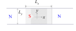
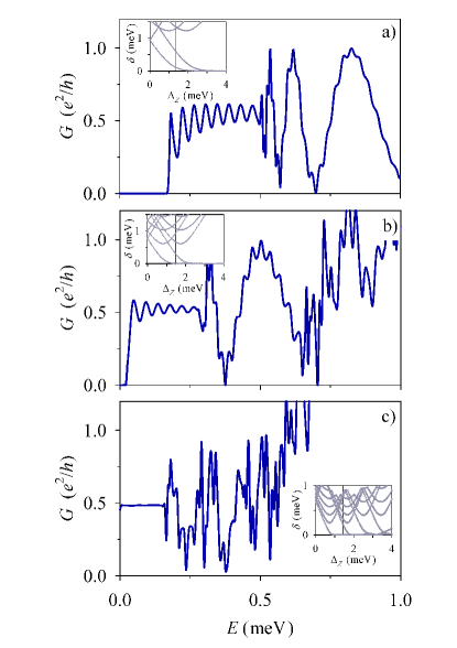
Figure 1: Upper: Sketch of the physical system. Panels a)-c): Conductance as a function of the energy (bias) for $L_{y}=1$ $\mu$m (a), 2 $\mu$m (b) and 5 $\mu$m (c). The three panels are for $L_{x}=20$ $\mu$m and $\Delta_{Z}=1.5$ meV. The insets in each panel show the $\delta-\Delta_{Z}$ phase diagram, with $\delta$ the $k=0$ gap of the $L_{x}\to\infty$ system. The vertical (red) line in each inset shows the correspondence with the energy sweep of its panel.

Method.- Our analysis is based on the numerical solution of the Bogoliubov-deGennes scattering equation ${\cal H}\Psi=E\Psi$ for a given energy $E$, assuming an expansion of the wave function in the complex band structure for each portion of the strip where the parameters are constant. An effective matching in 2d at the two interfaces of the NSN double junction yields all the scattering coefficients. The method is explained in more detail in the Supplemental Material SM and is based on Refs. Serra (2013); Osca and Serra (2015, 2017a, 2017b, 2018); Tisseur and Meerbergen (2001); Lehoucq et al. (1998); Lent and Kirkner (1990). In particular, the conductance for a given energy $E$ is determined as

$$G(E)=\frac{e^{2}}{h}\left[T_{N}(E)+R_{A}(E)\right]\;.$$ (2)

where $T_{N}$ is the normal (electron-electron) transmission probability and $R_{A}$ is the Andreev (electron-hole) reflection probability. The superconductor is assumed grounded and the applied bias symmetrical since otherwise currents may emerge from the superconductor and flow to the leads Lambert et al. (1993); Lim et al. (2012); Chung et al. (2011)

The resolution method describes both longitudinal and transverse evanescent behaviour, an essential point since we are interested in the dependence with both $L_{x}$ and $L_{y}$. Including large-enough sets of $N_{k}\approx 100$ complex-$k$ waves for each region describes longitudinal evanescent behaviour while a uniform $y$ spatial grid with $N_{y}\approx 100$ points is required to describe the transverse behavior. In addition, a minimal grid of only $N_{x}=5$ points for each interface is required for the matching. The computational cost is small and, quite importantly, it is independent of $L_{x}$, which is again essential for the study of the $L_{x}$-dependence up to large values.

Results.- Figure 1 shows a characteristic evolution of bias-dependent conductance, $G(E)$, as the strip width $L_{y}$ increases: 1 $\mu$m (a), 2 $\mu$m (b) and 5 $\mu$m (c). As expected, the wide strip shows a low-energy flat conductance of 0.5$e^{2}/h$ that, when increasing $E$, evolves into a complicated variation due to the successive activation of higher energy modes of the strip. The value of $\delta$, the $k=0$ gap energy, is shown for each mode as a funcion of $\Delta_{Z}$ in the corresponding insets of Fig. 1. In the narrower strips of Figs. 1a,b the flat 0.5$e^{2}/h$ plateau transforms into a clear oscillating pattern, with larger amplitude at the onset and gradually damping with increasing energies. This pattern is clearly enhanced in the smaller $L_{y}$ strip (Fig. 1a). A sudden change of this pattern occurs when a second chiral mode is activated, setting in a larger amplitude envelope oscillation between zero and one conductance quantum in Figs. 1a,b.

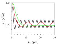
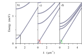
Figure 2: a) $L_{x}$ dependence of the conductance for different values of the width $L_{y}$, as indicated by the number close to each line (in microns). The results correspond to those in Fig. 1 for selected values of the energy: 0.3 meV ($L_{y}=1$ $\mu$m), 0.09 meV ($L_{y}=2$ $\mu$m), 0.1 meV ($L_{y}=5$ $\mu$m). b)-d): Energy bands for the corresponding values of $L_{y}$. The energy and wavenumber are indicated in each panel with the same line color of a).

The oscillating conductance in the regime of a single chiral mode of a narrow strip is the main result of this work. It is a sizeable effect, easily reaching 40-50 % conductance variations for energies near the activation onset of Fig. 1a. Next, we study the role of the longitudinal distance $L_{x}$ on the oscillation. Figure 2 shows $G(L_{x})$ corresponding to selected transverse widths and energies of Fig. 1. This figure provides a quantitative measure of the contribution of longitudinal evanescent modes to the conductance. In all cases $G$ initially decreases from a value close to one, reaching a sustained regime after a critical value of $L_{x}$ is exceeded. In the narrower strips the asymptotic-$L_{x}$ regime again reproduces the oscillating pattern mentioned above.

The separation between successive conductance maxima (minima) of the sustained oscillations of Fig. 2a can be related to the speed of the chiral Majorana mode. This connection is clear from a direct comparison between the computed real band structure of the propagating modes shown in Fig. 2b-d. The approximate Majorana mode is represented by the lowest band with an almost linear dependence on wavenumber, $E\approx c\hbar k$, with $c\approx 0.26\,{\rm meV}\mu{\rm m}/\hbar$. Assuming a conductance maximum requires an integer number of half wavelengths fit in distance $L_{x}$ we infer $c=\Delta L_{x}E/\pi$, where $\Delta L_{x}$ is the separation of two successive maxima. This reproduces $c\approx 0.26\,{\rm meV}\mu{\rm m}/\hbar$ for the $L_{y}=1\,\mu$m and $2\,\mu$m results of Fig. 2a, respectively.

As explicitly shown above, measuring $G(L_{x})$ allows an electrical determination of the mode speed. The same conclusion is obtained inferring $c$ from the separation energy $\Delta E$ between two successive maxima of the oscillation pattern $G(E)$ of Fig. 1a,b. In this case, however, the oscillation is not sustained for arbitrary large values, but one has to choose $E$ in the proper interval corresponding to the propagation of a single chiral mode. There is a clear analogy between our model system and a photon interferometer, similarly to other Condensed Matter systems such as Aharonov-Bohm rings, with the genuine difference that in a strip the interference of chiral modes is governed by the interplay between strip dimensions $L_{x}$, $L_{y}$ and the mechanism of Andreev backscattering. Incidentally, in units of the photon speed in vacuum the chiral mode speed of Fig. 2 is $\approx 1.3\times 10^{-3}$.

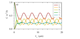
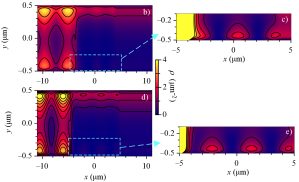
Figure 3: a) Evolution with $L_{x}$ of normal and Andreev reflections and transmissions for a strip of $L_{y}=1$ $\mu$m and energy $E=0.25$ meV. b-e) Spatial distribution of probability density, in $\mu{\rm m}^{-2}$, corresponding to the conductance maximum at $L_{x}=7.5\,\mu$m (b) and minimum at $L_{x}=9.3\,\mu$m (d). Panels c) and e) show the densities in a 10x-zoomed scale for the highlighted regions.

We now elucidate from our calculations the physical mechanism behind the enhanced conductance when condition $L_{x}=n\lambda/2$ is fulfilled, with $n$ an integer and $\lambda$ the wavelength of the chiral mode between the two interfaces. Figure 3 shows that the conductance oscillation basically reflects the behavior of the Andreev reflection probability $R_{A}$, the normal transmission $T_{N}$ is also oscillating but with a weaker amplitude and a reduced wavelength. The contour plots displayed in panels b)-e) show the distribution of quasiparticle probability density corresponding to an incidence from the upper left chiral mode. As expected, in the superconducting piece of the strip transmission proceeds predominantly attached to the upper edge. A zoom of the lower edge reveals that in panel c) two full intervals between density maxima fit in $L_{x}$, counting backwards from the lower right maximum, while in panel e) two and a half intervals can fit in. As the distance between density maxima is $\lambda/2$, this is the interference of the backscattered chiral mode from the right interface that can thus enhance/decrease the global Andreev reflection from the left interface.

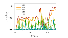
Figure 4: $G(E)$ in presence of barriers to the left and right of the strip superconductor region. The different curves correspond to varying barrier lengths $L_{b}$, as indicated in microns. We take $m_{0b}=2$ meV in the barrier sections of the strip. Other parameters as in Fig. 1b.

Edge chiral Majorana modes are robust against backscattering induced by local disorder, in a similar way of the quantum Hall effect. We have checked (Supplemental Material) that the conductance oscillations of this work are indeed robust with the presence of local fluctuations $\delta m_{0}(x,y)$ in a portion of the strip modelling bulk disorder as well as deviations from perfect straight edges. As final result, we have considered the presence of side material barriers in the longitudinal direction by assuming $m_{0}\equiv m_{0b}=2$ meV in regions of length $L_{b}$ to the left and right of the superconductor central island of the strip. As with usual potential barriers, the transparency of those side regions can be tuned by changing $m_{0b}$ and/or $L_{b}$. The presence of side barriers tends to decouple leads and central island, leading to a more clear manifestation of the interferometer character discussed above. Figure 4 shows how the oscillating pattern of $G(E)$ evolves to a sequence of spikes as the barriers become less and less transparent; each spike signaling the condition of resonant backscattering of the chiral Majorana mode. Thus, the configuration with side barriers suggests a device operation with more clear difference between its on and off states.

Conclusion.- In summary, our calculations suggest that a quantum-anomalous Hall thin strip with a central superconductor section could display conductance oscillations when the strip transverse size $L_{y}$ is in the micrometer range and the system is in a fully quantum coherent regime. As a function of the superconductor region length $L_{x}$ the oscillations are sustained up to arbitrary large values. We conclude that a quantum mesoscopic strip behaves as an interferometer that allows measuring the speed of the chiral Majorana mode. The physical mechanism is the enhanced Andreev reflection due to resonant backscattering of the chiral mode from the second to the first interface. The presence of side barriers magnifies the interferometer effect by yielding conductance spikes.

Supplemental Material

We give details of the method we use to solve the Bogoliubov-deGennes equation for quasiparticle scattering. Some complementary results are also included.

Appendix A Method

As discussed in the main text, we devise an approach to solve the scattering Bogoliubov-deGennes equation for quasiparticles

$${\cal H}\Psi(xy\eta_{\sigma}\eta_{\tau}\eta_{\lambda})=E\Psi(xy\eta_{\sigma}\eta_{\tau}\eta_{\lambda})\;,$$ (3)

where the $\eta$’s represent the doubled variables for spin, isospin and pseudospin, respectively. The main idea is to expand the wave function using the complex band structure for each portion of the wire and, subsequently, solve an effective set of equations ensuring the proper matching of solutions in 2d at the two longitudinal interfaces. Related solution schemes have been previously used by us in Refs. Serra (2013); Osca and Serra (2017a, b).

A.1 Complex $k$’s

In each uniform region (along $x$) we may expand

$$\Psi(xy\eta_{\sigma}\eta_{\tau}\eta_{\lambda})=\sum_{c}c_{k}\,e^{ik(x-x_{k})}\,\Phi_{k}(y\eta_{\sigma}\eta_{\tau}\eta_{\lambda})\;,$$ (4)

where the $\Phi_{k}$’s are the solutions of the translationally invariant problem for a characteristic wavenumber $k$. The phases $\exp{(-ikx_{k})}$ are introduced for convenience by a proper choice of the $x_{k}$’s, to be mentioned below. It is important to include the possibility of complex wavenumbers $k$ in order to describe evanescent modes. The sets of solutions $\{k,\Phi_{k}\}$ are determined from

$$(h(k)-E)\Phi_{k}(y\eta_{\sigma}\eta_{\tau}\eta_{\lambda})=0\;,$$ (5)

where $h(k)$ is the reduced Hamiltonian once the $x$ dependence has been removed assuming a plane wave along $x$.

Equation (5) can be seen as a nonlinear eigenvalue problem for $k$ (notice that $E$ is known). The kinetic-like term of the Hamiltonian yields a $k^{2}$ contribution, while the Rashba-like term yields a linear $k$ term. A clever transformation allows a simplification of Eq. (5) to a linear eigenvalue problem for $k$ by doubling the number of components of the wave function Tisseur and Meerbergen (2001). Defining $\tilde{\Phi}_{k}(y\eta_{\sigma}\eta_{\tau}\eta_{\lambda}\eta_{g})$ where $\eta_{g}$ is the new (generalized) double valued index, such that

$$\tilde{\Phi}_{k}(y\eta_{\sigma}\eta_{\tau}\eta_{\lambda}\eta_{g})=\left\{\begin{array}[]{cc}\rule{0.0pt}{2.84544pt}\Phi_{k}(y\eta_{\sigma}\eta_{\tau}\eta_{\lambda})&{\rm if}\;\eta_{g}=1\;,\\ \rule{0.0pt}{2.84544pt}\ell_{0}\,k\,s(\eta_{\tau})\Phi_{k}(y\eta_{\sigma}\eta_{\tau}\bar{\eta}_{\lambda})&{\rm if}\;\eta_{g}=2\;,\end{array}\right.$$ (6)

where $\ell_{0}$ is our length unit and we have defined $\bar{\eta}$ to be the opposite of $\eta$ and $s(\eta)=\pm 1$ for $\eta=1,2$, respectively. The resulting eigenvalue equation for $\tilde{\Phi}_{k}$ reads

$$\tilde{h}\,\tilde{\Phi}_{k}(y\eta_{\sigma}\eta_{\tau}\eta_{\lambda}\eta_{g})=k\,\tilde{\Phi}_{k}(y\eta_{\sigma}\eta_{\tau}\eta_{\lambda}\eta_{g})\;,$$ (7)

where $\tilde{h}$ is the corresponding generalized Hamiltonian, not depending on wavenumber, and $k$ is now a standard (linear) eigenvalue.

Discretizing the $y$ coordinate in a uniform grid of $N_{y}$ points and using finite differences for the derivatives Eq. (7) transforms into a matrix problem. The corresponding matrix is non Hermitian, as could be anticipated since $k$ can be complex. We have diagonalized it using the ARPACK inverse coding routines, which allow a very efficient use of the matrix sparseness Lehoucq et al. (1998). The method yields the set of $N_{k}$ wave numbers closer to a chosen value, typically $k=0$.

A.2 Matching in 2d

Having obtained a large enough set of complex $k$’s and $\Phi_{k}$’s in each part of the strip, next step requires matching the solutions using the apropriate boundary conditions; a process that will determine the $c_{k}$’s containing the physical information of the scattering matrix. Our approach is inspired by the quantum-transmitting-boundary method Lent and Kirkner (1990). We introduce a minimal $x$ grid of $N_{x}$ points centered around the positions of the two longitudinal interfaces. $N_{x}$ equals the number of points of the finite-difference rule for the derivatives. Typically, $N_{x}=3$ is enough, although we have also checked higher values $N_{x}=5,7,\dots$.

The algorithm has to define a closed set of equations for the unknowns

$$\left\{{c_{k}}^{\prime}s,\Psi(xy\eta_{\sigma}\eta_{\tau}\eta_{\lambda})\right\}\;,$$ (8)

where the $k$’s are those of output modes ($N_{k}$). The total number of unknowns in the unknowns set of Eq. (8) is $N_{k}+2\times 8N_{x}N_{y}$. The corresponding closed set of equations yielding all the unknowns is summarized in Tab. 1, where we have defined the projected equations

$$\sum_{\eta_{\sigma}\eta_{\tau}\eta_{\lambda}}\int{dy}\,\Phi_{k^{\prime}}^{*}(y\eta_{\sigma}\eta_{\tau}\eta_{\lambda})\,\Psi(xy\eta_{\sigma}\eta_{\tau}\eta_{\lambda}) =$$

$$\sum_{k}{c_{k}e^{ik(x-x_{k})}{\cal M}_{k^{\prime}k}}\;,$$ (9)

with the mode-overlap matrix

$${\cal M}_{k^{\prime}k}=\sum_{\eta_{\sigma}\eta_{\tau}\eta_{\lambda}}\int{dy}\,\Phi_{k^{\prime}}^{*}(y\eta_{\sigma}\eta_{\tau}\eta_{\lambda})\,\Phi_{k}(y\eta_{\sigma}\eta_{\tau}\eta_{\lambda})\;.$$ (10)

The resulting set of linear equations from Tab. 1 is solved using again the ARPACK routines. This has to be repeated for each input mode in order to determine the full scattering probabilities for arbitrary incidence. In each case, the solutions fulfil conservation of quasiparticle probability. Since the $x$-grids are defined only around the interfaces, the computational burden is not increasing with $L_{x}$. Finally, the $x_{k}$’s in Eq. (4) are chosen such that for complex wavenumbers the exponentially increasing solutions always remain bounded.

Table 1: Summary of effective 2d matching equations

	Number of Eqs.
Discretized Eq. (3) on central points of $x$-derivative rule	$2\times 8N_{y}$
Eq. (4) on side points of $x$-derivative rule	$2\times 8(N_{x}-1)N_{y}$
Projected Eq. (9) on central points of $x$-derivative rule	$N_{k}$

Appendix B Results

The following pages contain additional results not included in the main text.

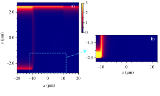
Figure 5: Same as Fig. 3d,e of the main text but for a wide strip of $L_{y}=5\;\mu$m, $L_{x}=20\,\mu$m and $E=0.1$ meV. The zoomed scale shows that chiral mode backscattering has fully vanished in between the two interfaces. Notice also that, relative to the tranverse size $L_{y}$, the edge-character of the modes is much increased while oscillations along $x$ are absent. We have used a $y$ grid with $N_{y}=200$ points. This case already agrees with the macroscopic result, with a flat conductance $G=0.5\,e^{2}/h$.

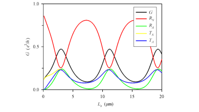
Figure 6: $G(L_{x})$ in presence of lateral material barriers with $m_{0b}=2\,{\rm meV}$ and $L_{b}=0.5\,\mu{\rm m}$. We have assumed $L_{y}=2\,\mu{\rm m}$, $E=0.1\,{\rm meV}$ and $\Delta_{Z}=1.5\,{\rm meV}$. As discussed in the main text with the case of $G(E)$, due to the barriers the conductance oscillations evolve to a sequence of peaks also with $G(L_{x})$.

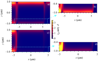
Figure 7: Same as Fig. 3 of the main text but for a strip of $L_{y}=2\;\mu$m with side barriers of $m_{0b}=2$ meV and $L_{b}=0.5\,\mu{\rm m}$. Panels a,b are for a conductance maximum (Fig. 6) with $L_{x}=11.2\,\mu$m, while panels c,d are for a conductance minimum (Fig. 6) with $L_{x}=7.4\,\mu$m. The zoom in density scale of panels b,d is 3x. As expected, the backscattered mode from the second to the first interface is much weaker in panel d) than in b).

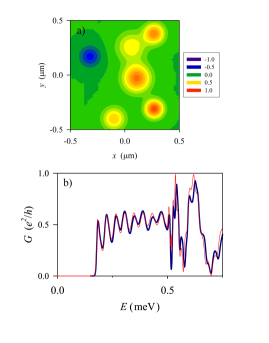
Figure 8: Same result of Fig. 1a of the main text in presence of impurities modeled as a fluctuating field $\delta m_{0}(x,y)$. We assumed a fluctuation range $\delta m_{0}/m_{0}\in[-1,1]$. a) Spatial distribution of $\delta m_{0}(x,y)$; b) comparison of the conductance in presence (thick) and absence (thin) of the impurities.

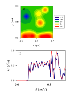
Figure 9: Same as Fig 8 with an extra accumulation of impurities on the lower edge of the strip that models a perturbation of the straight edge.