Wild Residual Bootstrap Inference for Penalized Quantile Regression with Heteroscedastic Errors

Abstract

We consider a heteroscedastic regression model in which some of the regression coefficients are zero but it is not known which ones. Penalized quantile regression is a useful approach for analyzing such data. By allowing different covariates to be relevant for modeling conditional quantile functions at different quantile levels, it provides a more complete picture of the conditional distribution of a response variable than mean regression. Existing work on penalized quantile regression has been mostly focused on point estimation. Although bootstrap procedures have recently been shown to be effective for inference for penalized mean regression, they are not directly applicable to penalized quantile regression with heteroscedastic errors. We prove that a wild residual bootstrap procedure for unpenalized quantile regression is asymptotically valid for approximating the distribution of a penalized quantile regression estimator with an adaptive $L_{1}$ penalty and that a modified version can be used to approximate the distribution of $L_{1}$-penalized quantile regression estimator. The new methods do not need to estimate the unknown error density function. We establish consistency, demonstrate finite sample performance, and illustrate the applications on a real data example.

1 Introduction

We consider the quantile regression model $Y_{i}={x}_{i}^{T}\mbox{$\beta$}_{0}+\epsilon_{i}$ ($i=1,\ldots,n$), where ${x}_{i}=(x_{i0},x_{i1},\ldots,x_{ip})^{T}$ with $x_{i0}=1$ is the $i$th nonstochastic design point in $\mathcal{R}^{p}$, and $\epsilon_{i}$ is a random error with probability density $f_{i}$ and the $\tau$th quantile equal to zero. The unknown regression coefficient $\mbox{$\beta$}_{0}=(\beta_{00},\beta_{01},\ldots,\beta_{0p})^{T}$ may depend on $\tau$, but we omit such dependence in notation for simplicity. Quantile regression was proposed by Koenker and Bassett, (1978) and has become a popular alternative to least squares regression. Conditional quantiles are of interest in a variety of applications, such as the conditional median of medical expenditure or a low conditional quantile of birth weight. Comparing such quantiles for a range of $\tau$ values enables researchers to obtain a more complete picture of the conditional distribution than mean regression and is particularly useful for analyzing heterogeneous data. See Koenker, (2005) and Koenker et al., (2017).

We suppose that some of the covariates are irrelevant for modeling the $\tau$th conditional quantile but we have no prior information on which. In such a setting, penalized quantile regression has been proven to avoid over-fitting by shrinking the estimated coefficients of irrelevant covariates toward zero. Here, we focus on the asymptotic regime where the number of predictors $p$ is fixed while the sample size $n$ goes to infinity. Asymptotic theory for penalized quantile regression in this setup was recently studied by Zou and Yuan, (2008) for independent and identically distributed random errors, and Wu and Liu, (2009), who established the asymptotic distribution of penalized quantile regression estimator for the adaptive $L_{1}$ penalty (Zou,, 2006) and considered an extension to the general heteroscedastic error setting. However, these works have not considered estimation of the standard error of the estimated penalized quantile regression coefficients. The asymptotic distribution of $L_{1}$-penalized quantile regression has a positive probability mass at zero for the component for which the true regression parameter has a zero value. Inference based directly on asymptotic theory is not convenient. On the other hand, the adaptively $L_{1}$-penalized quantile regression estimator enjoys the oracle property under regularity conditions: the zero coefficients are estimated as exactly zero with probability approaching unity and the nonzero coefficients have the asymptotic normal distribution we would obtain if we knew in advance which coefficients are zero. However, convergence to the oracle distribution is often slow and results in inaccurate confidence intervals (Chatterjee and Lahiri,, 2013).

In practice, a two-step procedure is commonly used to construct confidence intervals. First, penalized quantile regression is applied to select variables. Then the model is refitted with selected variables only to construct confidence intervals. Such a procedure does not account for uncertainties involved in variable selection and generally tends to produce wider confidence intervals, as demonstrated in our simulation study.

These challenges motivate us to develop a wild residual bootstrap-based inference approach for penalized quantile regression with $L_{1}$ or adaptive $L_{1}$ penalty. Our work is mostly related to Chatterjee and Lahiri, (2010, 2011, 2013) and Camponovo, (2015) on bootstrapping penalized estimators in the least squares regression setting. An alternative perturbation method for inference on regularized regression estimates was studied in Minnier et al., (2011). Chatterjee and Lahiri, (2010) proved that standard bootstrap is inconsistent for estimating the distribution of the $L_{1}$ penalized least squares estimator when one or more of the components of the regression parameter vector are zero; the failure of the naive paired bootstrap was proved in Camponovo, (2015). Modified residual and paired bootstraps were proposed in Chatterjee and Lahiri, (2011) and Camponovo, (2015), respectively. Chatterjee and Lahiri, (2013) demonstrated that although the adaptively penalized least squares estimator enjoys the oracle property, inference based directly on the oracle distribution is often inaccurate and more accurate inference can be obtained via a residual bootstrap. However, these bootstrap methods do not directly apply to the quantile regression setting due to the nonsmoothness of the quantile loss function and the heteroscedastic error distribution. We prove that a wild residual bootstrap procedure proposed by Feng et al., (2011) for unpenalized quantile regression is asymptotically valid for approximating the distribution of the quantile regression estimator with adaptive $L_{1}$ penalty. Furthermore, a modified version of this wild residual bootstrap procedure can be used to approximate the distribution of $L_{1}$ penalized quantile regression. Our derivation of the bootstrap consistency theory for penalized quantile regression uses techniques substantially different from that of Feng et al., (2011).

2 Inference for adaptive $L_{1}$-penalized quantile regression

2.1 Quantile regression with adaptive $L_{1}$ penalty

The unpenalized quantile regression estimator for $\mbox{$\beta$}_{0}$ is $\overline{\mbox{$\beta$}}=(\overline{\beta}_{0},\ldots,\overline{\beta}_{p})^{T}$, where

$$\overline{\mbox{$\beta$}}=\operatorname*{arg\,min}_{\mbox{$\beta$}}\sum_{i=1}^{n}\rho_{\tau}(Y_{i}-{x}_{i}^{T}\mbox{$\beta$})$$ (1)

and $\rho_{\tau}(u)=u\left\{\tau-I(u<0)\right\}$ is the quantile loss function. Under general regularity conditions, $\overline{\beta}$ is asymptotically normal. The asymptotic covariance matrix of $\overline{\beta}$ depends on the unknown conditional density function of $\epsilon_{i}$ (Koenker,, 2005).

Often not all covariates collected are relevant for modeling the $\tau$th conditional quantile, that is, some of the components of $\mbox{$\beta$}_{0}$ are zero. Let $A=\{1\leq j\leq p:\beta_{0j}\neq 0\}$ be the index set of the nonzero coefficients. Let $|A|=q$ be the cardinality of the set $A$. Without loss of generality, we assume that the last $p-q$ components of $\mbox{$\beta$}_{0}$ are zero; that is, we can write $\mbox{$\beta$}_{0}=(\mbox{$\beta$}_{01}^{T},{0}^{T}_{p-q})^{T}$, where ${0}_{p-q}$ denotes a $(p-q)$- dimensional vector of zeros, and $A=\{1,\ldots,q\}$. Let ${X}=({x}_{1},\ldots,{x}_{n})^{T}$ be the $n\times(p+1)$ matrix of covariates, where ${x}_{1}^{T},\ldots,{x}_{n}^{T}$ are the rows of ${X}$. We also write $X=({1},{X}_{1},\ldots,{X}_{p})$, where ${1},{X}_{1},\ldots,{X}_{p}$ are the columns of ${X}$ and ${1}$ represents an $n$-vector of ones. Define ${X}_{A}$ to be the submatrix of ${X}$ that consists of its first $q+1$ columns; and define ${X}_{A^{c}}$ to be the submatrix of ${X}$ that consists of its last $p-q$ columns. Similarly, let ${x}_{iA}$ be the subvector that contains the first $q+1$ entries of ${x}_{i}$.

The quantile regression estimator with the adaptive $L_{1}$ penalty performs simultaneous estimation and variable selection by minimizing a penalized quantile loss function, i.e.,

$$\widetilde{\mbox{$\beta$}}=\operatorname*{arg\,min}_{\mbox{$\beta$}}\Big{\{}\sum_{i=1}^{n}\rho_{\tau}(Y_{i}-{x}_{i}^{T}\mbox{$\beta$})+\lambda_{n}\sum_{j=1}^{p}w_{j}|\beta_{j}|\Big{\}},$$ (2)

where $\lambda_{n}>0$ is a tuning parameter, and $w_{j}=|\overline{\beta}_{j}|^{-\gamma}$ are the adaptive weights ($\gamma>0$). Write $\widetilde{\mbox{$\beta$}}=(\widetilde{\beta}_{0},\ldots,\widetilde{\beta}_{p})^{T}$ and $\widetilde{A}=\{1\leq j\leq p:\widetilde{\beta}_{j}\neq 0\}$. Let $\widetilde{\mbox{$\beta$}}_{1}$ be the subvector that contains the first $(q+1)$ elements of $\widetilde{\mbox{$\beta$}}$. Let $D_{0}=\lim_{n\rightarrow\infty}n^{-1}\sum_{i=1}^{n}{x}_{iA}{x}_{iA}^{T}$ and $D_{1}=\lim_{n\rightarrow\infty}n^{-1}\sum_{i=1}^{n}f_{i}(0){x}_{iA}{x}_{iA}^{T}$, where $f_{i}(0)$ is the density function of $\epsilon_{i}$ evaluated at zero. The following properties of $\widetilde{\mbox{$\beta$}}$ were established in Wu and Liu, (2009).

Lemma 2.1

Assume Condition 2 of Section 2.2 is satisfied. If $n^{-1/2}\lambda_{n}\rightarrow 0$ and $n^{(\gamma-1)/2}\lambda_{n}\rightarrow\infty$, then the adaptive $L_{1}$-penalized quantile regression estimator $\widetilde{\mbox{$\beta$}}$ enjoys the oracle property. That is,
(i) $\mbox{pr}(\widetilde{A}=A)\rightarrow 1$ as $n\rightarrow\infty$;
(ii) $n^{1/2}(\widetilde{\mbox{$\beta$}}_{1}-\mbox{$\beta$}_{01})\rightarrow N\{{0}_{q+1},\tau(1-\tau)D_{1}^{-1}D_{0}D_{1}^{-1}\}$ in distribution as $n\rightarrow\infty$.

The result in Lemma 1 is referred to as the oracle property: with probability approaching one the zero coefficients of $\mbox{$\beta$}_{0}$ are identified as zero and the nonzero coefficients are identified as nonzero; and we can estimate the nonzero subvector of $\mbox{$\beta$}_{0}$ as efficiently as if we know the true model in advance. The proof of Lemma 2.1 is given in the Supplementary Material.

2.2 A wild residual bootstrap procedure and its consistency

We use a wild residual bootstrap procedure to approximate the asymptotic distribution of $\widetilde{\mbox{$\beta$}}$. Our procedure is motivated by the work of Feng et al., (2011) for unpenalized quantile regression. To obtain the wild bootstrap sample, we follow the steps below.

1. We first calculate the residuals from the adaptively penalized quantile regression: $\hat{\epsilon}_{i}=Y_{i}-{x}_{i}^{T}\widetilde{\mbox{$\beta$}}$ ($i=1,\ldots,n$) and obtain $\widetilde{\mbox{$\beta$}}$ by (2).

2. Let $\epsilon_{i}^{*}=r_{i}|\hat{\epsilon}_{i}|$, where $r_{i}$ ($i=1,\ldots,n$) are generated as a random sample from a distribution with a cumulative distribution function $G$ satisfying Conditions 3-5 below.

3. We generate the bootstrap sample as $Y_{i}^{*}={x}_{i}^{T}\widetilde{\mbox{$\beta$}}+\epsilon_{i}^{*}$ ($i=1,\ldots,n$).

Using the bootstrap sample, we recalculate the adaptively penalized quantile regression estimator as

$$\widetilde{\mbox{$\beta$}}^{*}=\operatorname*{arg\,min}_{\mbox{$\beta$}}\Big{\{}\sum_{i=1}^{n}\rho_{\tau}(Y_{i}^{*}-{x}_{i}^{T}\mbox{$\beta$})+\lambda_{n}\sum_{j=1}^{p}w_{j}^{*}|\beta_{j}|\Big{\}},$$ (3)

where $w_{j}^{*}=|\overline{\beta}_{j}^{*}|^{-\gamma}$, $\overline{\mbox{$\beta$}}^{*}=(\overline{\beta}^{*}_{0},\ldots,\overline{\beta}^{*}_{p})^{T}$ is the ordinary quantile regression estimator recomputed on the bootstrap sample. For $j=1,\ldots,p$ and $0<\alpha<1$, let $d_{j}^{*(\alpha/2)}$ and $d_{j}^{*(1-\alpha/2)}$ be the $(\alpha/2)$-th and $(1-\alpha/2)$-th quantiles of the bootstrap distribution of $n^{1/2}(\widetilde{\mbox{$\beta$}}_{j}^{*}-\widetilde{\mbox{$\beta$}}_{j})$, respectively. We can estimate $d_{j}^{*(\alpha/2)}$ and $d_{j}^{*(1-\alpha/2)}$ from a large number of bootstrap samples. An asymptotic $100(1-\alpha)\%$ bootstrap confidence interval for $\beta_{0j}$, $j=1,\ldots,p$, is given by $\big{[}\widetilde{\mbox{$\beta$}}_{j}-n^{-1/2}d_{j}^{*(1-\alpha/2)},\widetilde{\mbox{$\beta$}}_{j}-n^{-1/2}d_{j}^{*(\alpha/2)}\big{]}.$ As in Feng et al., (2011), we work under the following technical conditions:
Condition 1. The true value $\mbox{$\beta$}_{0}$ is an interior point of a compact set in $R^{p}$. The density of $\epsilon_{i}$, denoted by $f_{i}(\cdot)$, is Lipschitz continuous and is bounded away from 0 and $\infty$ in a neighborhood around 0 for all $i$;
Condition 2. $\lim_{n\rightarrow\infty}n^{-1}\sum_{i=1}^{n}{x}_{i}{x}_{i}^{T}\rightarrow B_{0}$ and $\lim_{n\rightarrow\infty}n^{-1}\sum_{i=1}^{n}f_{i}(0){x}_{i}{x}_{i}^{T}\rightarrow B_{1}$ for some positive definite matrices $B_{0}$ and $B_{1}$. Furthermore, $\sum_{i=1}^{n}||{x}_{i}||^{3}=O(n)$ and $\max_{1\leq i\leq n}||{x}_{i}||=O(n^{1/4})$, where $||\cdot||$ is the Euclidean norm;
Condition 3. for some strictly positive constants $c_{1}$ and $c_{2}$, $\sup\{r\in\mathbb{G}:r\leq 0\}=-c_{1}$ and $\inf\{r\in\mathbb{G}:r\geq 0\}=c_{2}$, where $\mathbb{G}$ is the support of the weight distribution $G$;
Condition 4. the weight distribution $G$ satisfies $\int_{0}^{+\infty}r^{-1}dG(r)=-\int_{-\infty}^{0}r^{-1}dG(r)=1/2$ and $E_{G}(|r|)<\infty$ , where the expectation is taken under $G$;
Condition 5. the $\tau$th quantile of the distribution $G$ is zero.

Theorem 2.2 shows that the conditional distribution of $n^{1/2}(\widetilde{\mbox{$\beta$}}^{*}-\widetilde{\mbox{$\beta$}})$ provides an asymptotically valid approximation of that of $n^{1/2}(\widetilde{\mbox{$\beta$}}-\mbox{$\beta$})$. Let $\widetilde{A}^{*}=\{j=1,\ldots,p:\widetilde{\beta}_{j}^{*}\neq 0\}$, and let $\widetilde{\mbox{$\beta$}}_{1}^{*}$ be the subvector that contains the first $q+1$ elements of $\widetilde{\mbox{$\beta$}}^{*}$. Let ${r}=\{r_{1},\ldots,r_{n}\}$ be the random bootstrap weights and ${z}=\{{z}_{1},\ldots,{z}_{n}\}$ be the random sample. By the wild bootstrap mechanism, the distribution of ${r}$ is independent of that of ${z}$. Let $\mbox{pr}_{{z}}$ denote the probability under the joint distribution of ${z}$, and let $\mbox{pr}_{{r}\mid{z}}$ denote the probability of ${r}$ conditional on ${z}$.

Theorem 2.2

If Conditions 1–5 and the assumptions of Lemma 2.1 are satisfied, then $pr_{{r}\mid{z}}(\widetilde{A}^{*}=A)=1+o_{\textnormal{pr}_{{z}}}(1)$. Furthermore,

$$\sup_{t}\big{|}\textnormal{pr}_{{r}\mid{z}}\{n^{1/2}(\widetilde{\mbox{$\beta$}}_{1}^{*}-\widetilde{\mbox{$\beta$}}_{1})\leq t\}-\textnormal{pr}_{{z}}\{n^{1/2}(\widetilde{\mbox{$\beta$}}_{1}-\mbox{$\beta$}_{01})\leq t\}\big{|}=o_{\textnormal{pr}_{{z}}}(1).$$

Remark 1

Conditions 1 and 2 are slightly weaker than the corresponding conditions in Feng et al., (2011). Under Condition 5, conditional on the data, $\epsilon_{i}^{*}$ has the $\tau$th quantile equal to zero. Conditions 3 and 4 ensure that the asymptotic distribution of the bootstrap estimator, conditional on the data, matches the unconditional asymptotic distribution of the original adaptively penalized quantile regression estimator, which depends on the unknown error density function. A simple weight distribution that satisfies Conditions 3–5 is the two-point distribution with probabilities $1-\tau$ and $\tau$ at $r=2(1-\tau)$ and $-2\tau$, respectively. Another example given in Feng et al., (2011) is the distribution which for $1/8<\tau<7/8$, $g(r)=G^{\prime}(r)=-rI(-2\tau-1/4\leq r\leq-2\tau+1/4)+rI\{2(1-\tau)-1/4\leq r\leq 2(1-\tau)+1/4\}.$ We propose several other distributions that satisfy these conditions in the Supplementary Material.

Remark 2

By definition $n^{1/2}(\widetilde{\mbox{$\beta$}}^{*}-\widetilde{\mbox{$\beta$}})$ minimizes $Q_{n}^{*}(\mbox{$\delta$})$, where $Q_{n}^{*}(\mbox{$\delta$})=\sum_{i=1}^{n}\big{\{}\rho_{\tau}(\epsilon_{i}^{*}-n^{-1/2}{x}_{i}^{T}\mbox{$\delta$})-\rho_{\tau}(\epsilon_{i}^{*})\big{\}}+\lambda_{n}\sum_{j=1}^{p}w_{j}^{*}\big{(}\widetilde{\beta}_{j}+n^{-1/2}\delta_{j}|-|\widetilde{\beta}_{j}|\big{)},$ The crux of the proof of Theorem 2.2 is to show that conditional on the data,

$$Q_{n}^{*}(\mbox{$\delta$})\rightarrow Q^{*}(\mbox{$\delta$})=\begin{cases}-\mbox{$\delta$}^{T}H+\mbox{$\delta$}^{T}B_{1}\mbox{$\delta$}/2,&\text{ $\delta_{j}=0$ for $j>q$},\\ +\infty,&\text{otherwise},\end{cases}$$

in probability, where $H\sim N\{{0},\tau(1-\tau)B_{0}\}$. Then the results follow from epi-convergence theory, see the unpublished technical reports of Geyer (On the asymptotics of convex stochastic optimization, technical report, 1996) and Knight (Epi-convergence in distribution and stochastic equi-semicontinuity, technical report, 1999).

Remark 3

As pointed out by a referee, Leeb and Pötscher, (2008) and Pötscher and Schneider, (2009) revealed that the distribution of adaptive lasso and other shrinkage-type estimators cannot be estimated uniformly in a shrinking neighborhood of the underlying parameter values. In the setting we consider, the number of covariates is fixed. We assume the smallest nonzero signal is not diminishing to zero when the sample size increases. Furthermore, as in Chatterjee and Lahiri, (2011), we do not claim the bootstrap based estimator of the distribution of adaptive lasso to be uniformly consistent over any diminishing neighborhood of underlying parameter values. See also Remark 3 of Chatterjee and Lahiri, (2011).

Remark 4

For the adaptive lasso, the coverage probability of the confidence interval approaches unity, because the wild residual bootstrap distribution approximates the adaptive lasso estimator distribution, which identifies zero coefficients as exactly zero with probability approaching unity.

3 Modified wild residual bootstrap for $L_{1}$ penalized quantile regression

We also consider the $L_{1}$ or lasso penalized quantile regression estimator

$$\widecheck{\mbox{$\beta$}}=\operatorname*{arg\,min}_{\mbox{$\beta$}}\Big{\{}\sum_{i=1}^{n}\rho_{\tau}(Y_{i}-{x}_{i}^{T}\mbox{$\beta$})+\lambda_{n}\sum_{j=1}^{p}|\beta_{j}|\Big{\}},$$ (4)

where $\lambda_{n}>0$ is a tuning parameter. The asymptotic distribution of $\widecheck{\mbox{$\beta$}}$ follows that of the minimizer of a random process, which is specified in the following lemma.

Lemma 3.1

Under Condition 2 and if $n^{-1/2}\lambda_{n}\rightarrow\lambda_{0}\geq 0$,

$$n^{1/2}(\widecheck{\mbox{$\beta$}}-\mbox{$\beta$}_{0}) \rightarrow \operatorname*{arg\,min}_{\mbox{$\delta$}}\Big{[}-\mbox{$\delta$}^{T}H+\mbox{$\delta$}^{T}B_{1}\mbox{$\delta$}/2+\lambda_{0}\sum_{j=1}^{p}\big{\{}|\delta_{j}|I(\beta_{0j}=0)$$

$$\hskip 56.9055pt+\delta_{j}\mathrm{sign}(\beta_{0j})I(\beta_{0j}\neq 0)\big{\}}\Big{]},$$

in distribution as $n\rightarrow\infty$, where $H$ is defined in Remark 2.

The proof is given in the Supplementary Material. For $L_{1}$-penalized mean regression, Chatterjee and Lahiri, (2010) proved that the asymptotic distribution of the naive residual bootstrapped lasso estimator is a random measure on $R^{p}$ and that the bootstrap is inconsistent whenever the regression parameter vector contains one or more zeros. An explanation of this phenomenon is that the lasso estimates the sign of nonzero coefficients correctly with high probability, but estimates the zero coefficients to be positive or negative with positive probabilities. The naive residual bootstrap fails to reproduce the sign of zero coefficients with high probability. To remedy this, Chatterjee and Lahiri, (2010) proposed a thresholding procedure, which we adapt.

Our procedure proceeds as follows. Let $\{a_{n}\}$ be a sequence of numbers such that $a_{n}+(n^{-1/2}\log n)a_{n}^{-1}\rightarrow 0$ as $n\rightarrow\infty$. For example, $a_{n}=cn^{-\delta}$, for some $c>0$, $0<\delta<1/2$. For $\overline{\mbox{$\beta$}}$ defined in (1), we consider the thresholded estimator $\widecheck{\mbox{$\beta$}}^{*}=(\widecheck{\beta}^{*}_{0},\ldots,\widecheck{\beta}^{*}_{p})^{T}$, where $\widecheck{\beta}^{*}_{0}=\overline{\beta}_{0}$ and $\widecheck{\beta}^{*}_{j}=\widecheck{\beta}_{j}I(|\widecheck{\beta}_{j}|>a_{n})$ for $j=1\ldots,p$. Let $\widecheck{\epsilon}_{i}=Y_{i}-{x}_{i}^{T}\widecheck{\mbox{$\beta$}}^{*}$ ($i=1,\ldots,n$). Let $\epsilon_{i}^{**}=r_{i}|\widecheck{\epsilon}_{i}|$ ($i=1,\ldots,n$), where the bootstrap weights $r_{i}$ satisfy Conditions 3–5. We choose to threshold the ordinary quantile regression estimator directly. Alternatively, we may threshold the lasso estimator $\widecheck{\mbox{$\beta$}}$, which will yield the same asymptotic results for the bootstrapped estimator but requires an additional tuning parameter for the lasso.

The bootstrap sample is generated by $Y_{i}^{**}={x}_{i}^{T}\widecheck{\mbox{$\beta$}}^{*}+\epsilon_{i}^{**}$ ($i=1,\ldots,n$). We then recalculate the $L_{1}$ penalized quantile regression estimator using the bootstrap sample:

$$\widecheck{\mbox{$\beta$}}^{**}=\operatorname*{arg\,min}_{\mbox{$\beta$}}\Big{\{}\sum_{i=1}^{n}\rho_{\tau}(Y_{i}^{**}-{x}_{i}^{T}\mbox{$\beta$})+\lambda_{n}\sum_{j=1}^{p}|\beta_{j}|\Big{\}}.$$ (5)

Theorem 3.2 below shows that the conditional distribution of $n^{1/2}(\widecheck{\mbox{$\beta$}}^{**}-\widecheck{\mbox{$\beta$}}^{*})$ provides an asymptotically valid approximation of that of $n^{1/2}(\widecheck{\mbox{$\beta$}}-\mbox{$\beta$}_{0})$.

Theorem 3.2

If Conditions 1–5 and the assumptions of Lemma 3.1 are satisfied, then

$$\sup_{t}\big{|}\textnormal{pr}_{{r}\mid{z}}\{n^{1/2}(\widecheck{\mbox{$\beta$}}^{**}-\widecheck{\mbox{$\beta$}}^{*})\leq t\}-\textnormal{pr}_{{z}}\{n^{1/2}(\widecheck{\mbox{$\beta$}}-\mbox{$\beta$}_{0})\leq t\}\big{|}=o_{\textnormal{pr}_{{z}}}(1).$$

4 Numerical results

4.1 Monte Carlo studies

We study the accuracy of 95% confidence intervals constructed by our bootstrap procedures. For the adaptive $L_{1}$ penalty, we select the tuning parameter $\lambda_{n}$ by minimizing a Bayesian information criterion (Lee et al.,, 2014) and consider $\gamma=1,2$. For the $L_{1}$ penalty, we select $\lambda_{n}$ by cross-validation and consider two choices of $a_{n}$. One choice adopts a data-driven approach that minimizes the estimated mean squared error $E^{*}(||\widecheck{\mbox{$\beta$}}^{**}-\widecheck{\mbox{$\beta$}}^{*}||^{2})$, where $E^{*}$ is the average over bootstrap samples; see Section 5.2 of Chatterjee and Lahiri, (2011) and Remark 2 of Camponovo, (2015). The other choice is the empirical choice $a_{n}=n^{-1/3}$, which is motivated by the rate required by the asymptotic theory. The bootstrap random weights $r_{i}$ are generated from the two-point distribution described in Feng et al., (2011); see Remark 1. We also tried alternative weight distributions and found the results similar.

We compare the new methods with the confidence intervals from the oracle model, from the full model, and from the two-step procedure described in Section 1 with adaptive lasso or lasso applied in the first step. The oracle procedure is not implementable in real data analysis. For these competing methods, we consider confidence intervals obtained by the rank score method and by the wild bootstrap method in the R package quantreg (Koenker,, 2016).

Table 1: Empirical coverage probabilities ($\times 100$) and average interval lengths (in parentheses) for nominal 95% confidence intervals

	$\beta_{1}=\Phi^{-1}(\tau)$	$\beta_{3}=$0$\cdot$25	$\beta_{5}=$0$\cdot$5	$\beta_{7}=1$	$\beta_{9}=2$	Zeros	TP	FP
			$\tau=$0$\cdot$5	$n=100$
New AL1	92$\cdot$0 (0$\cdot$33)	94$\cdot$6 (0$\cdot$15)	93$\cdot$2 (0$\cdot$17)	95$\cdot$3 (0$\cdot$13)	92$\cdot$7 (0$\cdot$14)	97$\cdot$4 (0$\cdot$06)	4	0$\cdot$3
New AL2	90$\cdot$6 (0$\cdot$42)	95$\cdot$0 (0$\cdot$15)	93$\cdot$6 (0$\cdot$17)	95$\cdot$1 (0$\cdot$13)	92$\cdot$5 (0$\cdot$14)	98$\cdot$3 (0$\cdot$06)	4	0$\cdot$3
New L1	90$\cdot$7 (0$\cdot$28)	92$\cdot$9 (0$\cdot$15)	92$\cdot$4 (0$\cdot$18)	94$\cdot$9 (0$\cdot$15)	91$\cdot$2 (0$\cdot$16)	93$\cdot$5 (0$\cdot$11)	4	3$\cdot$3
New L2	92$\cdot$2 (0$\cdot$29)	93$\cdot$7 (0$\cdot$16)	93$\cdot$6 (0$\cdot$19)	96$\cdot$1 (0$\cdot$16)	94$\cdot$5 (0$\cdot$17)	95$\cdot$5 (0$\cdot$12)	4	3$\cdot$3
Full RS	94$\cdot$8 (0$\cdot$59)	95$\cdot$9 (0$\cdot$21)	96$\cdot$7 (0$\cdot$24)	96$\cdot$2 (0$\cdot$21)	96$\cdot$1 (0$\cdot$22)	95$\cdot$9 (0$\cdot$21)	4	6
Full WB	91$\cdot$0 (0$\cdot$54)	97$\cdot$4 (0$\cdot$18)	95$\cdot$9 (0$\cdot$22)	97$\cdot$6 (0$\cdot$18)	94$\cdot$6 (0$\cdot$20)	96$\cdot$1 (0$\cdot$19)	4	6
TS AL RS	94$\cdot$8 (0$\cdot$51)	96$\cdot$6 (0$\cdot$21)	96$\cdot$3 (0$\cdot$27)	97$\cdot$1 (0$\cdot$23)	95$\cdot$6 (0$\cdot$23)	98$\cdot$2 (0$\cdot$26)	4	0$\cdot$3
TS AL WB	91$\cdot$5 (0$\cdot$47)	95$\cdot$5 (0$\cdot$16)	94$\cdot$2 (0$\cdot$21)	96$\cdot$0 (0$\cdot$17)	92$\cdot$4 (0$\cdot$19)	97$\cdot$7 (0$\cdot$21)	4	0$\cdot$3
TS L RS	94$\cdot$1 (0$\cdot$52)	96$\cdot$2 (0$\cdot$22)	95$\cdot$6 (0$\cdot$27)	96$\cdot$0 (0$\cdot$23)	95$\cdot$4 (0$\cdot$24)	96$\cdot$3 (0$\cdot$26)	4	3$\cdot$3
TS L WB	92$\cdot$1 (0$\cdot$49)	94$\cdot$7 (0$\cdot$18)	94$\cdot$3 (0$\cdot$22)	95$\cdot$9 (0$\cdot$19)	93$\cdot$3 (0$\cdot$20)	95$\cdot$8 (0$\cdot$21)	4	3$\cdot$3
Oracle RS	-	97$\cdot$1 (0$\cdot$21)	97$\cdot$9 (0$\cdot$26)	97$\cdot$0 (0$\cdot$20)	97$\cdot$2 (0$\cdot$18)	-	4	0
Oracle WB	-	97$\cdot$7 (0$\cdot$15)	95$\cdot$9 (0$\cdot$19)	98$\cdot$2 (0$\cdot$15)	97$\cdot$2 (0$\cdot$16)	-	4	0
			$\tau=$0$\cdot$7	$n=250$
New AL1	89$\cdot$6 (0$\cdot$35)	94$\cdot$8 (0$\cdot$10)	92$\cdot$2 (0$\cdot$09)	94$\cdot$9 (0$\cdot$08)	93$\cdot$6 (0$\cdot$09)	98$\cdot$7 (0$\cdot$04)	5	0$\cdot$1
New AL2	89$\cdot$8 (0$\cdot$34)	94$\cdot$1 (0$\cdot$09)	91$\cdot$7 (0$\cdot$09)	95$\cdot$0 (0$\cdot$08)	93$\cdot$1 (0$\cdot$09)	99$\cdot$0 (0$\cdot$04)	5	0$\cdot$1
New L1	90$\cdot$1 (0$\cdot$34)	94$\cdot$4 (0$\cdot$10)	94$\cdot$2 (0$\cdot$10)	95$\cdot$4 (0$\cdot$08)	95$\cdot$1 (0$\cdot$09)	95$\cdot$4 (0$\cdot$06)	5	2$\cdot$6
New L2	90$\cdot$7 (0$\cdot$35)	94$\cdot$9 (0$\cdot$10)	94$\cdot$2 (0$\cdot$10)	95$\cdot$4 (0$\cdot$08)	95$\cdot$1 (0$\cdot$09)	95$\cdot$9 (0$\cdot$06)	5	2$\cdot$6
Full RS	94$\cdot$9 (0$\cdot$39)	96$\cdot$8 (0$\cdot$12)	95$\cdot$3 (0$\cdot$12)	95$\cdot$8 (0$\cdot$10)	96$\cdot$4 (0$\cdot$11)	95$\cdot$9 (0$\cdot$11)	5	5
Full WB	90$\cdot$6 (0$\cdot$37)	96$\cdot$3 (0$\cdot$11)	95$\cdot$5 (0$\cdot$11)	97$\cdot$3 (0$\cdot$09)	96$\cdot$1 (0$\cdot$11)	96$\cdot$2 (0$\cdot$10)	5	5
TS AL RS	93$\cdot$8 (0$\cdot$37)	95$\cdot$4 (0$\cdot$12)	96$\cdot$1 (0$\cdot$10)	95$\cdot$9 (0$\cdot$11)	96$\cdot$4 (0$\cdot$12)	98$\cdot$8 (0$\cdot$11)	5	0$\cdot$1
TS AL WB	91$\cdot$7 (0$\cdot$35)	95$\cdot$2 (0$\cdot$11)	95$\cdot$7 (0$\cdot$09)	95$\cdot$8 (0$\cdot$10)	96$\cdot$5 (0$\cdot$11)	98$\cdot$9 (0$\cdot$11)	5	0$\cdot$1
TS L RS	93$\cdot$8 (0$\cdot$37)	95$\cdot$0 (0$\cdot$12)	95$\cdot$3 (0$\cdot$11)	96$\cdot$2 (0$\cdot$11)	95$\cdot$5 (0$\cdot$12)	96$\cdot$1 (0$\cdot$11)	5	2$\cdot$6
TS L WB	91$\cdot$2 (0$\cdot$35)	94$\cdot$8 (0$\cdot$12)	95$\cdot$2 (0$\cdot$10)	95$\cdot$7 (0$\cdot$11)	96$\cdot$8 (0$\cdot$12)	96$\cdot$0 (0$\cdot$10)	5	2$\cdot$6
Oracle RS	94$\cdot$0 (0$\cdot$38)	96$\cdot$8 (0$\cdot$11)	95$\cdot$3 (0$\cdot$11)	95$\cdot$9 (0$\cdot$09)	96$\cdot$4 (0$\cdot$10)	-	5	0
Oracle WB	90$\cdot$8 (0$\cdot$36)	95$\cdot$7 (0$\cdot$10)	94$\cdot$9 (0$\cdot$10)	96$\cdot$6 (0$\cdot$08)	96$\cdot$4 (0$\cdot$10)	-	5	0

• New AL1: proposed method with adaptive $L_{1}$ penalty ($\gamma=1$); New AL2: proposed method with adaptive $L_{1}$ penalty ($\gamma=2$); New L1: proposed method with $L_{1}$ penalty (data-driven choice of $a_{n}$); New L2: proposed method with $L_{1}$ penalty ($a_{n}=n^{-1/3}$); Full RS: full model with rank-score method; Full WB: full model with wild residual bootstrap; TS AL RS: two-step procedure, adaptive $L_{1}$ ($\gamma=1$) followed by rank-score method; TS AL WB: two-step procedure, adaptive $L_{1}$ ($\gamma=1$) followed by wild residual bootstrap; TS L RS: two-step procedure, lasso followed by rank-score method; TS L WB: two-step procedure, lasso followed by wild residual bootstrap; Oracle RS: oracle model with rank-score method; Oracle WB: oracle model with wild residual bootstrap; Zeros: the reported average coverage probability (length) is the average for all zero coefficients; TP: average number of true positives; FP: average number of false positives.

Let $Y=$0$\cdot$25$X_{3}+$0$\cdot$5$X_{5}+X_{7}+2X_{2}+X_{1}\xi,$ where $\xi\sim N(0,1)$ denotes the random error. Let $\widetilde{X}=(\widetilde{X}_{1},\dots,\widetilde{X}_{10})^{T}\sim N_{10}(0,I_{p})$. We set $X_{1}=\Phi(\widetilde{X}_{1})$, where $\Phi$ is the standard normal cumulative distribution function, and $X_{i}=\widetilde{X}_{i}$ for $i=2,\dots,10$. We consider estimating the conditional median and the 0$\cdot$7 conditional quantile of $Y$. Note that the variable $X_{1}$ is inactive for estimating the conditional median and is active for estimating the 0$\cdot$7 conditional quantile. Let $\mbox{$\beta$}=(\beta_{1},\ldots,\beta_{10})^{T}$ be the vector of quantile regression coefficients. We have $\beta_{3}=$0$\cdot$25, $\beta_{5}=$0$\cdot$5, $\beta_{7}=1$, $\beta_{9}=2$, $\beta_{2}=\beta_{4}=\beta_{6}=\beta_{8}=\beta_{10}=0$ for both quantiles, $\beta_{1}=0$ for the conditional median and $\beta_{1}=\Phi^{-1}$(0$\cdot$7) for the 0$\cdot$7 conditional quantile.

We perform 1000 simulations with 400 bootstrapped samples for each. We report sample size $n=100$ for estimating the conditional median and size 250 for estimating the 0$\cdot$7 conditional quantile, as it is known to be more challenging to estimate a higher quantile than to estimate the median. Table 1 summarizes the simulation results. The standard errors of the coverage probabilities are below 0.01 and the standard errors of the confidence interval lengths are below 0.005 for all cases. We also report the average number of nonzero coefficients correctly identified to be nonzero and the average number of zero coefficients incorrectly identified to be nonzero. For the two-step procedure, we only report results for $\gamma=1$ if adaptive lasso is applied in Step 1 as the results for $\gamma=2$ are similar. Additional simulation results are given in the Supplementary Material.

The wild residual bootstrap procedures achieve the specified coverage probability. For the $L_{1}$ penalty, the two choices of $a_{n}$ yield similar results. The adaptive $L_{1}$ penalty produces sparser models than the $L_{1}$ penalty does. The resulting confidence intervals are generally shorter than those based on the full model or the two-step procedure. For the adaptive lasso, the coverage probability of the confidence interval for zero coefficients is close to one, see Remark 4. Similar numerical findings for adaptive lasso penalized least square regression were reported in Minnier et al. (2011) and Camponovo (2015).

4.2 A real data example

We analyze data on the effects of ozone on school children’s lung growth (Ihorst et al.,, 2004). The study was carried out from February 1996 to October 1999 in South Western Germany on school children initially in first and second primary school classes. The data we analyze contain a subset of 496 children with complete data at three examinations (Buchholz et al.,, 2008).

The response variable is the forced vital capacity of the lung. We consider the ten explanatory variables with the largest inclusion probabilities using the bootstrap procedure from De Bin et al., (2015): gender, $x_{1}$; height at pulmonary function testing, $x_{2}$; weight at pulmonary function testing, $x_{3}$; maximal nitrogen oxide value of last 24 hours before pulmonary function testing, $x_{4}$; wheezing or whistling in the chest, $x_{5}$; shortness of breath, $x_{6}$; whether patient lives in a village with high ozone values, $x_{7}$; sensitization to pollens, $x_{8}$; sensitization to dust mite allergens, $x_{9}$; and age at March 1, 1996, $x_{10}$.

Table 2 reports 95% confidence intervals for each covariate from bootstrapping penalized quantile regression with the adaptive $L_{1}$ and $L_{1}$ penalties for estimating the conditional median and the conditional 0.7 quantile. For both methods, the variables $x_{1}$, $x_{2}$ and $x_{3}$ are identified as significant at both quantiles.

Table 2: Analysis of ozone data: wild residual-based 95% bootstrapped confidence intervals for the 0.5 and 0.7 conditional quantiles

	$\tau=$0$\cdot$5					$\tau=$0$\cdot$7
	New AL1	New AL2	New L		New AL1	New AL2	New L
Intercept	(2$\cdot$26, 2$\cdot$31)	(2$\cdot$26, 2$\cdot$30)	(2$\cdot$26, 2$\cdot$31)		(2$\cdot$37, 2$\cdot$41)	(2$\cdot$37, 2$\cdot$41)	(2$\cdot$37, 2$\cdot$42)
$x_{1}$	($-$0$\cdot$13, $-$0$\cdot$08)	($-$0$\cdot$12, $-$0$\cdot$09)	($-$0$\cdot$10, $-$0$\cdot$10)		($-$0$\cdot$12, $-$0$\cdot$08)	($-$0$\cdot$12, $-$0$\cdot$08)	($-$0$\cdot$10, $-$0$\cdot$10)
$x_{2}$	(0$\cdot$15, 0$\cdot$22)	(0$\cdot$14, 0$\cdot$20)	(0$\cdot$18, 0$\cdot$24)		(0$\cdot$16, 0$\cdot$22)	(0$\cdot$16, 0$\cdot$22)	(0$\cdot$21, 0$\cdot$26)
$x_{3}$	(0$\cdot$04, 0$\cdot$12)	(0$\cdot$05, 0$\cdot$12)	(0$\cdot$07, 0$\cdot$08)		(0$\cdot$06, 0$\cdot$15)	(0$\cdot$06, 0$\cdot$15)	(0$\cdot$08, 0$\cdot$09)
$x_{4}$	(0, 0)	($-$0$\cdot$01, 0$\cdot$01)	(0, 0)		($-$0$\cdot$01, 0)	($-$0$\cdot$01, 0)	(0, 0)
$x_{5}$	(0, 0)	(0$\cdot$01, 0$\cdot$03)	(0$\cdot$02, 0$\cdot$02)		($-$0$\cdot$01, 0)	($-$0$\cdot$01, 0)	(0, 0)
$x_{6}$	(0, 0)	(0, 0)	(0, 0)		(0$\cdot$01, 0$\cdot$05)	(0$\cdot$01, 0$\cdot$05)	(0$\cdot$03, 0$\cdot$03)
$x_{7}$	(0, 0)	($-$0$\cdot$01, 0$\cdot$01)	(0, 0)		(0, 0$\cdot$01)	($-$0$\cdot$01, 0$\cdot$01)	(0, 0)
$x_{8}$	(0, 0)	($-$0$\cdot$01, 0$\cdot$01)	(0, 0)		($-$0$\cdot$03, $-$0$\cdot$01)	($-$0$\cdot$03, 0)	($-$0$\cdot$02, $-$0$\cdot$02)
$x_{9}$	(0, 0)	($-$0$\cdot$01, 0$\cdot$01)	(0, 0)		(0, 0$\cdot$02)	(0, 0$\cdot$02)	(0, 0)
$x_{10}$	(0, 0)	(0, 0$\cdot$04)	(0$\cdot$01, 0$\cdot$02)		(0, 0$\cdot$01)	(0, 0$\cdot$01)	($-$0$\cdot$01, 0)

• New AL1: proposed method with adaptive $L_{1}$ penalty ($\gamma=1$); New AL2: proposed method with adaptive $L_{1}$ penalty ($\gamma=2$); and New L: proposed method with $L_{1}$ penalty (data-driven choice of $a_{n}$).

Appendix: Proofs of Theorems 2.2 and 3.2

We use $E^{*}$ and $\mbox{var}^{*}$ to denote expectation and variance conditional on the sample ${z}$. Let $E_{{r},{z}}$ and $\mbox{var}_{{r},{z}}$ be the expectation and variance with respect to the joint distribution of ${r}$ and ${z}$. Let pr denote the probability under the joint distribution; and let $\mbox{pr}_{{r}\mid{z}}$ denote the probability of ${r}$ conditional on ${z}$. A random variable $R_{n}$ is said to be $o_{p_{{r}}}^{*}(1)$ if for any $\epsilon,\delta>0$, $\mbox{pr}_{{z}}\{\mbox{pr}_{{r}|{z}}(|R_{n}|>\epsilon)>\delta\}\rightarrow 0$, as $n\rightarrow\infty$, and $o_{\mbox{pr}_{{r},{z}}}(1)$ is the regular notion with respect to the joint distribution of ${r}$ and ${z}$. Lemma 3 from Cheng and Huang, (2010) will be used repeatedly to allow for the transition of various stochastic orders in different probability spaces.

Let $V_{n}^{*}(\mbox{$\delta$})=\sum_{i=1}^{n}\big{\{}\rho_{\tau}(\epsilon_{i}^{*}-n^{-1/2}{x}_{i}^{T}\mbox{$\delta$})-\rho_{\tau}(\epsilon_{i}^{*})\big{\}}.$ Let $\psi_{\tau}(u)=\tau-I(u<0)$. It follows from Knight, (1998) and Koenker, (2005) that

$$V_{n}^{*}(\mbox{$\delta$}) = -n^{-1/2}\sum_{i=1}^{n}{x}_{i}^{T}\mbox{$\delta$}\psi_{\tau}(\epsilon_{i}^{*})+\sum_{i=1}^{n}\int_{0}^{n^{-1/2}{x}_{i}^{T}\mbox{$\delta$}}\big{\{}I(\epsilon_{i}^{*}\leq s)-I(\epsilon_{i}^{*}\leq 0)\big{\}}ds$$

$$= V_{1n}^{*}(\mbox{$\delta$})+V_{2n}^{*}(\mbox{$\delta$}).$$

Lemma .1

Under the conditions of Theorem 2.2,

$$\sup_{t}\big{|}\textnormal{pr}_{{r}\mid{z}}\{V_{1n}^{*}(\mbox{$\delta$})\leq t\}-\textnormal{pr}_{{z}}\{-\mbox{$\delta$}^{T}H\leq t\}\big{|}=o_{\textnormal{pr}_{{z}}}(1).$$ (6)

The proof of Lemma A1 is given in the Supplementary Material.

Lemma .2

Under the conditions of Theorem 2.2,

$$V_{2n}^{*}(\mbox{$\delta$})=\mbox{$\delta$}^{T}B_{1}\mbox{$\delta$}/2+o_{p_{{r}}}^{*}(1).$$ (7)

Proof. Recall $\epsilon_{i}^{*}=r_{i}|\hat{\epsilon}_{i}|$ and $\hat{\epsilon}_{i}=\epsilon_{i}-{x}_{i}^{T}(\widetilde{\mbox{$\beta$}}-\mbox{$\beta$}_{0})$. We will show that

$$\sup_{{b}\in B}|V_{2n}^{*}(\mbox{$\delta$},{b})-\mbox{$\delta$}^{T}B_{1}\mbox{$\delta$}/2|=o_{p_{{r}}}^{*}(1),$$

where $V_{2n}^{*}(\mbox{$\delta$},{b})=\sum_{i=1}^{n}\int_{0}^{n^{-1/2}{x}_{i}^{T}\mbox{$\delta$}}\big{\{}I(r_{i}|\epsilon_{i}-n^{-1/2+\eta}{x}_{i}^{T}{b}|\leq s)-I(r_{i}\leq 0)\big{\}}ds,$ with $B$ a compact set and $\eta>0$. Since $\mbox{pr}_{{z}}\{n^{1/2-\eta}(\widetilde{}\mbox{$\beta$}-\mbox{$\beta$}_{0})\in B\}\rightarrow 1$, the result of the lemma follows. By Lemma 3 of Cheng and Huang, (2010), it suffices to show that

$$\sup_{{b}\in B}|V_{2n}^{*}(\mbox{$\delta$},{b})-\mbox{$\delta$}^{T}B_{1}\mbox{$\delta$}/2|=o_{p_{{r},{z}}}(1).$$

We will use Theorem 2.11.9 in van der Vaart and Wellner, (1996). For a fixed $\varepsilon>0$, divide the set $B$ in $O(\varepsilon^{-2p})$ cubes of the form $C_{k}=\prod_{j=1}^{p}[b_{j,k_{j}-1},b_{j,k_{j}})$ with ${k}=(k_{1},\ldots,k_{p})^{T}$, $k_{j}=1,\ldots,O(\varepsilon^{-2})$ for $j=1,\ldots,p$, and $b_{j,k_{j}}-b_{j,k_{j}-1}\leq\varepsilon^{2}$. Then, writing $V_{2n}^{*}(\mbox{$\delta$},{b})=\sum_{i=1}^{n}v_{i{b}}$, we will show that

$$\sum_{i=1}^{n}E_{{r},{z}}\Big{(}\sup_{{b},{b}^{\prime}\in C_{k}}|v_{i{b}}-v_{i{b}^{\prime}}|^{2}\Big{)}\leq\varepsilon^{2}.$$ (8)

Indeed, for fixed $i$ and for ${b},{b}^{\prime}\in C_{k}$, $|v_{i{b}}-v_{i{b}^{\prime}}|^{2}$ is bounded above by

$$\Big{|}\int_{0}^{n^{-1/2}{x}_{i}^{T}\mbox{$\delta$}}\big{\{}I(r_{i}|\epsilon_{i}-n^{-1/2+\eta}{x}_{i}^{T}{b}|\leq s)-I(r_{i}|\epsilon_{i}-n^{-1/2+\eta}{x}_{i}^{T}{b}^{\prime}|\leq s)\big{\}}ds\Big{|}^{2}$$

$$\leq \ I({x}_{i}^{T}\mbox{$\delta$}>0)n^{-1/2}{x}_{i}^{T}\mbox{$\delta$}\int_{0}^{n^{-1/2}{x}_{i}^{T}\mbox{$\delta$}}\big{|}I(r_{i}|\epsilon_{i}-n^{-1/2+\eta}{x}_{i}^{T}{b}|\leq s)-I(r_{i}|\epsilon_{i}-n^{-1/2+\eta}{x}_{i}^{T}{b}^{\prime}|\leq s)\big{|}ds$$

$$+I({x}_{i}^{T}\mbox{$\delta$}\leq 0)n^{-1/2}|{x}_{i}^{T}\mbox{$\delta$}|\int_{0}^{n^{-1/2}|{x}_{i}^{T}\mbox{$\delta$}|}\big{|}I(r_{i}|\epsilon_{i}-n^{-1/2+\eta}{x}_{i}^{T}{b}|\leq-s)-I(r_{i}|\epsilon_{i}-n^{-1/2+\eta}{x}_{i}^{T}{b}^{\prime}|\leq-s)\big{|}ds.$$

Let us focus on the first term above, as the second term is similar. The first term equals

$$I({x}_{i}^{T}\mbox{$\delta$}>0,r_{i}>0)n^{-1/2}{x}_{i}^{T}\mbox{$\delta$}\int_{0}^{n^{-1/2}{x}_{i}^{T}\mbox{$\delta$}}\big{|}I(-s/r_{i}+n^{-1/2+\eta}{x}_{i}^{T}{b}\leq\epsilon_{i}\leq s/r_{i}+n^{-1/2+\eta}{x}_{i}^{T}{b})$$

$$-I(-s/r_{i}+n^{-1/2+\eta}{x}_{i}^{T}{b}^{\prime}\leq\epsilon_{i}\leq s/r_{i}+n^{-1/2+\eta}{x}_{i}^{T}{b}^{\prime})\big{|}ds$$

$$\leq I({x}_{i}^{T}\mbox{$\delta$}>0,r_{i}>0)n^{-1/2}{x}_{i}^{T}\mbox{$\delta$}\int_{0}^{n^{-1/2}{x}_{i}^{T}\mbox{$\delta$}}\Big{\{}\big{|}I(\epsilon_{i}\leq s/r_{i}+n^{-1/2+\eta}{x}_{i}^{T}{b})-I(\epsilon_{i}\leq s/r_{i}+n^{-1/2+\eta}{x}_{i}^{T}{b}^{\prime})\big{|}$$

$$+\big{|}I(\epsilon_{i}\leq-s/r_{i}+n^{-1/2+\eta}{x}_{i}^{T}{b})-I(\epsilon_{i}\leq-s/r_{i}+n^{-1/2+\eta}{x}_{i}^{T}{b}^{\prime})\big{|}\Big{\}}ds$$

$$\leq I({x}_{i}^{T}\mbox{$\delta$}>0,r_{i}>0)n^{-1/2}{x}_{i}^{T}\mbox{$\delta$}\int_{0}^{n^{-1/2}{x}_{i}^{T}\mbox{$\delta$}}\Big{[}\big{\{}I(\epsilon_{i}\leq s/r_{i}+n^{-1/2+\eta}{x}_{i}^{T}{b}_{k})-I(\epsilon_{i}\leq s/r_{i}+n^{-1/2+\eta}{x}_{i}^{T}{b}_{{k}-1})\big{\}}$$

$$+\big{\{}I(\epsilon_{i}\leq-s/r_{i}+n^{-1/2+\eta}{x}_{i}^{T}{b}_{k})-I(\epsilon_{i}\leq-s/r_{i}+n^{-1/2+\eta}{x}_{i}^{T}{b}_{{k}-1})\big{\}}\Big{]}ds,$$

where for notational simplicity we assume that all components of ${x}_{i}$ are positive. Hence,

$$\sum_{i=1}^{n}E_{{r},{z}}\Big{(}\sup_{{b},{b}^{\prime}\in C_{k}}|v_{i{b}}-v_{i{b}^{\prime}}|^{2}\Big{)}$$

$$\leq n^{-1/2}\sum_{i=1}^{n}|{x}_{i}^{T}\mbox{$\delta$}|\int\int_{0}^{n^{-1/2}|{x}_{i}^{T}\mbox{$\delta$}|}\Big{[}\big{\{}F_{i}(s/r+n^{-1/2+\eta}{x}_{i}^{T}{b}_{k})-F_{i}(s/r+n^{-1/2+\eta}{x}_{i}^{T}{b}_{{k}-1})\big{\}}$$

$$\hskip 14.22636pt+\big{\{}F_{i}(-s/r+n^{-1/2+\eta}{x}_{i}^{T}{b}_{k})-F_{i}(-s/r+n^{-1/2+\eta}{x}_{i}^{T}{b}_{{k}-1})\big{\}}\Big{]}ds\,dG(r)$$

$$\leq 2n^{-1}\sum_{i=1}^{n}|{x}_{i}^{T}\mbox{$\delta$}|^{2}n^{-1/2+\eta}{x}_{i}^{T}|{b}_{k}-{b}_{{k}-1}|\sup_{t\in{\cal N}_{i}}f_{i}(t)\leq c\varepsilon^{2},$$

for some $0<c<\infty$, for $\eta\leq 1/2$, where ${\cal N}_{i}$ is a neighborhood of 0 such that $\sup_{t\in{\cal N}_{i}}f_{i}(t)<\infty$; see Condition 1. This verifies (8).

Let $N_{[\,]}(\varepsilon,B,L_{2}^{n})$ be the bracketing number of $B$, i.e., the minimal number of sets $N_{\varepsilon}$ in a partition $B=\cup_{j=1}^{N_{\varepsilon}}B_{\varepsilon j}$ such that $\sum_{i=1}^{n}E_{{r},{z}}\big{\{}\sup_{{b},{b}^{\prime}\in B_{\varepsilon j}}(v_{i{b}}-v_{i{b}^{\prime}})^{2}\big{\}}\leq\varepsilon^{2}$ for $j=1,\ldots,N_{\varepsilon}$. For any $\delta_{n}\downarrow 0$,

$$\int_{0}^{\delta_{n}}\{\log N_{[\,]}(\varepsilon,B,L_{2}^{n})\}^{1/2}\,d\varepsilon\leq c\int_{0}^{\delta_{n}}\{\log(\varepsilon^{-2p})\}^{1/2}d\varepsilon\rightarrow 0.$$

Since the partition of $B$ does not depend on $n$ and since $\sup_{{b}\in B}|v_{i{b}}|\rightarrow 0$ for all $i$, it follows from Theorem 2.11.9 in van der Vaart and Wellner, (1996) that $V_{2n}^{*}(\mbox{$\delta$},{b})-E_{{r},{z}}\{V_{2n}^{*}(\mbox{$\delta$},{b})\}$ converges weakly in $\ell^{\infty}(B)$ provided it converges marginally, where $\ell^{\infty}(B)$ is the space of bounded functions from $B$ to $\mathcal{R}$ equipped with the supremum norm.

To check convergence of $V_{2n}^{*}(\mbox{$\delta$},{b})$ for fixed ${b}\in B$, it suffices to show that $\mbox{E}_{{r},{z}}\{V_{2n}^{*}(\mbox{$\delta$},{b})\}\rightarrow\mbox{$\delta$}^{T}B_{1}\mbox{$\delta$}/2$ and $\mbox{var}_{{r},{z}}\{V_{2n}^{*}(\mbox{$\delta$},{b})\}\rightarrow 0$. Note that

$$E_{{r},{z}}\{V_{2n}^{*}(\mbox{$\delta$},{b})\}$$

$$= E_{{r}}\Big{(}E_{{z}|{r}}\Big{[}\sum_{i=1}^{n}\int_{0}^{n^{-1/2}{x}_{i}^{T}\mbox{$\delta$}}\big{\{}I(r_{i}|\epsilon_{i}-n^{-1/2+\eta}{x}_{i}^{T}{b}|\leq s)-I(r_{i}\leq 0)\big{\}}ds\Big{]}\Big{)}$$

$$= \int_{0}^{\infty}\sum_{i=1}^{n}\int_{0}^{n^{-1/2}{x}_{i}^{T}\mbox{$\delta$}}\big{\{}F_{i}(s/r+n^{-1/2+\eta}{x}_{i}^{T}{b})-F_{i}(-s/r+n^{-1/2+\eta}{x}_{i}^{T}{b})\big{\}}I({x}_{i}^{T}\mbox{$\delta$}>0)dsdG(r)$$

$$+\int_{-\infty}^{0}\sum_{i=1}^{n}\int_{0}^{n^{-1/2}{x}_{i}^{T}\mbox{$\delta$}}\big{\{}1-F_{i}(s/r+n^{-1/2+\eta}{x}_{i}^{T}{b})+F_{i}(-s/r+n^{-1/2+\eta}{x}_{i}^{T}{b})-1\big{\}}I({x}_{i}^{T}\mbox{$\delta$}<0)dsdG(r)$$

$$=W_{1}+W_{2},$$

say, where $F_{i}$ denotes the distribution of $\epsilon_{i}$.

$$W_{1} = \int_{0}^{\infty}\sum_{i=1}^{n}\int_{0}^{n^{-1/2}{x}_{i}^{T}\mbox{$\delta$}}\big{\{}f_{i}(0)2s/r\big{\}}I({x}_{i}^{T}\mbox{$\delta$}>0)dsdG(r)$$

$$+\int_{0}^{\infty}\sum_{i=1}^{n}\int_{0}^{n^{-1/2}{x}_{i}^{T}\mbox{$\delta$}}\big{\{}f_{i}(t^{*}/r)-f_{i}(0)\big{\}}2s/rI({x}_{i}^{T}\mbox{$\delta$}>0)dsdG(r)=W_{11}+W_{12},$$

say, where $t^{*}$ is between $-n^{-1/2}{x}_{i}^{T}\mbox{$\delta$}+n^{-1/2+\eta}{x}_{i}^{T}{b}$ and $n^{-1/2}{x}_{i}^{T}\mbox{$\delta$}+n^{-1/2+\eta}{x}_{i}^{T}{b}$. Note that

$$W_{11}=\int_{0}^{\infty}r^{-1}dG(r)\sum_{i=1}^{n}f_{i}(0)\big{(}n^{-1/2}{x}_{i}^{T}\mbox{$\delta$}\big{)}^{2}I({x}_{i}^{T}\mbox{$\delta$}>0)=\frac{1}{2}\mbox{$\delta$}^{T}\big{\{}n^{-1}\sum_{i=1}^{n}f_{i}(0){x}_{i}{x}_{i}^{T}I({x}_{i}^{T}\mbox{$\delta$}>0)\big{\}}\mbox{$\delta$}.$$

By Condition 1, there exists a positive constant $c$ such that

$$|W_{12}| \leq c\int_{0}^{\infty}\sum_{i=1}^{n}\int_{0}^{n^{-1/2}{x}_{i}^{T}\mbox{$\delta$}}\big{(}n^{-1/2}{x}_{i}^{T}\mbox{$\delta$}/r+n^{-1/2+\eta}|{x}_{i}^{T}{b}|\big{)}2s/rI({x}_{i}^{T}\mbox{$\delta$}>0)dsdG(r)$$

$$\leq c\Big{\{}\int_{0}^{\infty}r^{-2}dG(r)\Big{\}}\big{(}n^{-1/2}||\mbox{$\delta$}||\max_{1\leq i\leq n}||{x}_{i}||\big{)}\Big{[}\mbox{$\delta$}^{T}\big{\{}n^{-1}\sum_{i=1}^{n}{x}_{i}{x}_{i}^{T}I({x}_{i}^{T}\mbox{$\delta$}>0)\big{\}}\mbox{$\delta$}\Big{]}$$

$$+c\Big{\{}\int_{0}^{\infty}r^{-1}dG(r)\Big{\}}\big{(}n^{-1/2+\eta}||{b}||\max_{1\leq i\leq n}||{x}_{i}||\big{)}\Big{[}\mbox{$\delta$}^{T}\big{\{}n^{-1}\sum_{i=1}^{n}{x}_{i}{x}_{i}^{T}I({x}_{i}^{T}\mbox{$\delta$}>0)\big{\}}\mbox{$\delta$}\Big{]}\rightarrow 0,$$

as Conditions 3 and 4 imply that $\int_{0}^{\infty}r^{-2}dG(r)$ is bounded, and by Condition 2 we have $n^{-1/2+\eta}\max_{1\leq i\leq n}||{x}_{i}||\rightarrow 0$ for $\eta$ small enough. Similarly, we can show $W_{2}=\frac{1}{2}\mbox{$\delta$}^{T}\big{\{}n^{-1}\sum_{i=1}^{n}f_{i}(0){x}_{i}{x}_{i}^{T}I({x}_{i}^{T}\mbox{$\delta$}<0)\big{\}}\mbox{$\delta$}+o(1).$ Hence, $E_{{r},{z}}\{V_{2n}^{*}(\mbox{$\delta$},{b})\}\rightarrow\mbox{$\delta$}^{T}B_{1}\mbox{$\delta$}/2$ as $n\rightarrow\infty$. To show $\mbox{var}_{{r},{z}}\{V_{2n}^{*}(\mbox{$\delta$},{b})\}\rightarrow 0$, we have

$$\mbox{var}_{{r},{z}}\{V_{2n}^{*}(\mbox{$\delta$},{b})\} = \sum_{i=1}^{n}\mbox{var}_{{r},{z}}\Big{[}\int_{0}^{n^{-1/2}{x}_{i}^{T}\mbox{$\delta$}}\big{\{}I(r_{i}|\epsilon_{i}-n^{-1/2+\eta}{x}_{i}^{T}{b}|\leq s)-I(r_{i}\leq 0)\big{\}}ds\Big{]}$$

$$\leq \sum_{i=1}^{n}E_{{r},{z}}\Big{[}\int_{0}^{n^{-1/2}{x}_{i}^{T}\mbox{$\delta$}}\big{\{}I(r_{i}|\epsilon_{i}-n^{-1/2+\eta}{x}_{i}^{T}{b}|\leq s)-I(r_{i}\leq 0)\big{\}}ds\Big{]}^{2}$$

$$= \Big{(}n^{-1/2}||\mbox{$\delta$}||\max_{1\leq i\leq n}||{x}_{i}||\Big{)}E_{{r},{z}}\{V_{2n}^{*}(\mbox{$\delta$},{b})\},$$

where the last equality follows because $\int_{0}^{n^{-1/2}{x}_{i}^{T}\mbox{$\delta$}}\big{\{}I(r_{i}|\epsilon_{i}-n^{-1/2+\eta}{x}_{i}^{T}{b}|\leq s)-I(r_{i}\leq 0)\big{\}}ds$ is always nonnegative. Since $n^{-1/2}\max_{1\leq n}||{x}_{i}||\rightarrow 0$ and $\mbox{E}_{{r},{z}}\{V_{2n}^{*}(\mbox{$\delta$},{b})\}\rightarrow\mbox{$\delta$}^{T}B_{1}\mbox{$\delta$}/2$, we have $\mbox{var}_{{r},{z}}\{V_{2n}^{*}(\mbox{$\delta$},{b})\}\rightarrow 0$ as $n\rightarrow\infty$. This finishes the proof. $\Box$

Proof of Theorem 2.2. Recall that $Q_{n}^{*}(\mbox{$\delta$})=\sum_{i=1}^{n}\big{\{}\rho_{\tau}(\epsilon_{i}^{*}-n^{-1/2}{x}_{i}^{T}\mbox{$\delta$})-\rho_{\tau}(\epsilon_{i}^{*})\big{\}}+\lambda_{n}\sum_{j=1}^{p}w_{j}^{*}\big{(}|\widetilde{\beta}_{j}+n^{1/2}\delta_{j}|-|\widetilde{\beta}_{j}|\big{)}$, where $w_{j}^{*}=|\overline{\beta}_{j}^{*}|^{-\gamma}$, $\overline{\mbox{$\beta$}}^{*}=(\overline{\beta}^{*}_{0},\overline{\beta}^{*}_{1},\ldots,\overline{\beta}^{*}_{p})^{T}$ is the ordinary quantile regression estimator computed from the bootstrap sample, $\gamma>0$. We have $n^{1/2}(\widetilde{\mbox{$\beta$}}^{*}-\widetilde{\mbox{$\beta$}})=\operatorname*{arg\,min}_{\mbox{$\delta$}}Q_{n}^{*}(\mbox{$\delta$}).$ Let $A_{n}$ denote the event that the adaptive lasso estimator $\widetilde{\mbox{$\beta$}}$ correctly estimated all the zero components of $\beta$, i.e., $A_{n}$ is the set of all $\omega\in\Omega$ such that $\{j:1\leq j\leq p,\widetilde{\beta}_{j}(\omega)=0\}=\{q+1,\ldots,p\}$. Then it follows from Lemma 2.1 that $\mbox{pr}(A_{n})\rightarrow 1$ as $n\rightarrow\infty$. There exists a subsequence $\{n_{k}\}$ such that $\mbox{pr}(A_{n_{k}}^{c}i.o.)=0$. Let $\Omega_{0}^{c}$ be the union of $\limsup_{k}A_{n_{k}}^{c}$ and the event on which (6) or (7) fails to hold, then $\mbox{pr}(\Omega_{0})=1$. For any fixed $w\in\Omega_{0}$, there exists $n_{w}\geq 1$ such that for all $n\geq n_{w}$, $\{j:1\leq j\leq p,\widetilde{\beta}_{nj}(\omega)=0\}=\{q+1,\ldots,p\}$. Hence on $\Omega_{0}$, as $n\rightarrow\infty$,

$$Q_{n}^{*}(\mbox{$\delta$})\rightarrow Q^{*}(\mbox{$\delta$})=\begin{cases}-\mbox{$\delta$}^{T}H+\mbox{$\delta$}^{T}B_{1}\mbox{$\delta$}/2,&\text{$\delta_{q+1}=\cdots=\delta_{p}=0$,}\\ +\infty,&\text{otherwise},\end{cases}$$

in probability. Following the same argument as in Lemma 2.1 and applying epi-convergence theory see the unpublished technical reports of Geyer (On the asymptotics of convex stochastic optimization, technical report, 1996) and Knight (Epi-convergence in distribution and stochastic equi-semicontinuity, technical report, 1999), the result is established by the equivalent representation of bootstrap consistency in (23.2) of van der Vaart, (1998). $\Box$
Proof of Theorem 3.2. Let $A_{n}=\{||\widecheck{\mbox{$\beta$}}^{*}-\mbox{$\beta$}_{0}||\leq cn^{-1/2}\log(n)\}$ for some given positive constant $c$. Since $\overline{\mbox{$\beta$}}$ is $n^{1/2}$-consistent, we have $\mbox{pr}(A_{n})\rightarrow 1$. Let $Q_{n}^{**}(\mbox{$\delta$})=\sum_{i=1}^{n}\big{\{}\rho_{\tau}(\epsilon_{i}^{**}-n^{-1/2}{x}_{i}^{T}\mbox{$\delta$})-\rho_{\tau}(\epsilon_{i}^{**})\big{\}}+\lambda_{n}\sum_{j=1}^{p}\big{(}|\widecheck{\beta}^{*}_{j}+n^{-1/2}\delta_{j}|-|\widecheck{\beta}^{*}_{j}|\big{)},$ then $n^{1/2}(\widecheck{\mbox{$\beta$}}^{**}-\widecheck{\mbox{$\beta$}}^{*})$ minimizes $Q_{n}^{**}(\mbox{$\delta$})$. Let $V_{n}^{**}(\mbox{$\delta$})=\sum_{i=1}^{n}\big{\{}\rho_{\tau}(\epsilon_{i}^{**}-{x}_{i}^{T}\mbox{$\delta$}/n^{1/2})-\rho_{\tau}(\epsilon_{i}^{**})\big{\}}.$ We can write

$$V_{n}^{**}(\mbox{$\delta$}) = -n^{-1/2}\sum_{i=1}^{n}{x}_{i}^{T}\mbox{$\delta$}\psi_{\tau}(\epsilon_{i}^{**})+\sum_{i=1}^{n}\int_{0}^{n^{-1/2}{x}_{i}^{T}\mbox{$\delta$}}\big{\{}I(\epsilon_{i}^{**}\leq s)-I(\epsilon_{i}^{**}\leq 0)\big{\}}ds$$

$$= V_{1n}^{**}(\mbox{$\delta$})+V_{2n}^{**}(\mbox{$\delta$}).$$

Similarly as in the proof of Lemma A1,

$$\sup_{t}\big{|}\textnormal{pr}_{{r}\mid{z}}\{V_{1n}^{**}(\mbox{$\delta$})\leq t\}-\textnormal{pr}_{{z}}\{-\mbox{$\delta$}^{T}H\leq t\}\big{|}=o_{\textnormal{pr}_{{z}}}(1).$$

Similarly as in the proof of Lemma A2, $V_{2n}^{**}(\mbox{$\delta$})=\mbox{$\delta$}^{T}B_{1}\mbox{$\delta$}/2+o_{p_{{r}}}^{*}(1).$ For $n$ sufficiently large, on the event $A_{n}$, $\mbox{sign}(\widecheck{\beta}^{*}_{j})=\mbox{sign}(\beta_{0j})$ and $\widecheck{\beta}^{*}_{j}=\overline{\beta}_{0j}$ for $j=1,\ldots,q$; and $\widecheck{\beta}^{*}_{j}=0$ for $j=q+1,\ldots,p$. Conditional on the data, $\lambda_{n}\sum_{j=1}^{p}\big{\{}|\widecheck{\beta}^{*}_{j}+\delta_{j}/n^{1/2}|-|\widecheck{\beta}^{*}_{j}|\big{\}}\rightarrow\lambda_{0}\sum_{j=1}^{p}\big{\{}|\delta_{j}|I(\widecheck{\beta}^{*}_{j}=0)+\delta_{j}\mbox{sign}(\beta_{0j})I(\widecheck{\beta}^{*}_{j}\neq 0)\}$. For any $1\leq j\leq p$,

$$\mbox{pr}\Big{\{}|\delta_{j}|I(\widecheck{\beta}^{*}_{j}=0)+\delta_{j}\mbox{sign}(\beta_{0j})I(\widecheck{\beta}^{*}_{j}\neq 0)=|\delta_{j}|I(\beta_{0j}=0)+\delta_{j}\mbox{sign}(\beta_{0j})I(\beta_{0j}\neq 0)\Big{\}}$$

$$\geq \mbox{pr}\Big{\{}|\delta_{j}|I(\widecheck{\beta}^{*}_{j}=0)+\delta_{j}\mbox{sign}(\beta_{0j})I(\widecheck{\beta}^{*}_{j}\neq 0)=|\delta_{j}|I(\beta_{0j}=0)+\delta_{j}\mbox{sign}(\beta_{0j})I(\beta_{0j}\neq 0),A_{n}\Big{\}}\rightarrow 1,$$

as $n\rightarrow\infty$. Therefore, conditional on the data, as $n\rightarrow\infty$,

$$Q_{n}^{**}(\mbox{$\delta$})\rightarrow-\mbox{$\delta$}^{T}H+\mbox{$\delta$}^{T}B_{1}\mbox{$\delta$}/2+\lambda_{0}\sum_{j=1}^{p}\big{\{}|\delta_{j}|I(\beta_{0j}=0)+\delta_{j}\mbox{sign}(\beta_{0j})I(\beta_{0j}\neq 0)\big{\}},$$

in distribution. Following the same argument as in Lemma 3.1 and applying epi-convergence theory, see the unpublished technical reports of Geyer (On the asymptotics of convex stochastic optimization, technical report, 1996) and Knight (Epi-convergence in distribution and stochastic equi-semicontinuity, technical report, 1999), the result is established by the equivalent representation of bootstrap consistency in (23.2) of van der Vaart, (1998). $\Box$

Supplementary Material

Appendix 1

Proofs of Lemma 1, Lemma 2 and Lemma A1

The proofs of Lemmas 1 and 2 combine the ideas in Wu and Liu, (2009) and Wang et al., (2012). Section 3.3 of Wu and Liu, (2009) considered an extension of the asymptotic theory of penalized quantile regression to the general heteroscedastic error setting but only a sketch of the derivation was provided in their online supplement. We provide a detailed derivation below for completeness.

Proof of Lemma 1. Write $\mbox{$\delta$}=(\mbox{$\delta$}_{1}^{T},\mbox{$\delta$}_{2}^{T})^{T}$, where $\mbox{$\delta$}_{1}=(\delta_{0},\delta_{1},\ldots,\delta_{q})^{T}$ and $\mbox{$\delta$}_{2}=(\delta_{q+1},\ldots,\delta_{p})^{T}$. Write $\widetilde{\mbox{$\delta$}}=(\widetilde{\mbox{$\delta$}}_{1}^{T},\widetilde{\mbox{$\delta$}}_{2}^{T})^{T}=n^{1/2}(\widetilde{\mbox{$\beta$}}-\mbox{$\beta$}_{0})$. Then $\widetilde{\mbox{$\delta$}}$ minimizes $Q_{n}(\mbox{$\delta$})$, where

$$Q_{n}(\mbox{$\delta$})=\sum_{i=1}^{n}\big{\{}\rho_{\tau}(\epsilon_{i}-n^{-1/2}{x}_{i}^{T}\mbox{$\delta$})-\rho_{\tau}(\epsilon_{i})\big{\}}+\lambda_{n}\sum_{j=1}^{p}w_{j}\big{(}|\beta_{0j}+n^{-1/2}\delta_{j}|-|\beta_{0j}|\big{)}.$$

It follows from Knight, (1998) and Koenker, (2005) that $\sum_{i=1}^{n}\big{\{}\rho_{\tau}(\epsilon_{i}-n^{-1/2}{x}_{i}^{T}\mbox{$\delta$})-\rho_{\tau}(\epsilon_{i})\big{\}}=-\mbox{$\delta$}^{T}H+\mbox{$\delta$}^{T}B_{1}\mbox{$\delta$}/2+o_{p}(1),$ where $H\sim N\{{0},\tau(1-\tau)B_{0}\}$. For the penalty term, we consider two cases. (i) For $j=1,\ldots,q$, $\overline{\beta}_{j}\rightarrow\beta_{0j}\neq 0$ in probability, and $n^{1/2}\big{(}|\beta_{0j}+\delta_{j}/n^{1/2}|-|\beta_{0j}|\big{)}\rightarrow\delta_{j}\mbox{sign}(\beta_{0j})$. It follows that $\lambda_{n}w_{j}\big{(}|\beta_{0j}+\delta_{j}/n^{1/2}|-|\beta_{0j}|\big{)}=(n^{-1/2}\lambda_{n})|\overline{\beta}_{0j}|^{-\gamma}n^{1/2}\big{(}|\beta_{0j}+\delta_{j}/n^{1/2}|-|\beta_{0j}|\big{)}\rightarrow 0$ as $n^{-1/2}\lambda_{n}\rightarrow 0$. (ii) For $j=q+1,\ldots,p$, $\lambda_{n}w_{j}\big{(}|\beta_{0j}+\delta_{j}/n^{1/2}|-|\beta_{0j}|\big{)}=(n^{(\gamma-1)/2}\lambda_{n})(n^{1/2}|\overline{\beta}_{j}|)^{-\gamma}|\delta_{j}|$. Since $n^{(\gamma-1)/2}\lambda_{n}\rightarrow\infty$ and $n^{1/2}|\overline{\beta}_{j}|=O_{p}(1)$, the limit of $\lambda_{n}w_{j}\big{(}|\beta_{0j}+\delta_{j}/n^{1/2}|-|\beta_{0j}|\big{)}$ is zero if $\delta_{j}=0$ and is $\infty$ if $\delta_{j}\neq 0$. Hence

$$Q_{n}(\mbox{$\delta$})\rightarrow Q(\mbox{$\delta$})=\begin{cases}-\mbox{$\delta$}^{T}H+\mbox{$\delta$}^{T}B_{1}\mbox{$\delta$}/2,&\delta_{q+1}=\cdots=\delta_{p}=0,\\ +\infty,&\text{otherwise},\end{cases}$$

in probability. Note that $Q_{n}(\mbox{$\delta$})$ is convex in $\delta$ and its limit $Q(\mbox{$\delta$})$ has a unique minimum $(D_{1}^{-1}W,{0}_{p-q}^{T})^{T}$, where $W\sim N\{0,\tau(1-\tau)D_{0}\}$, $D_{0}=\lim_{n\rightarrow\infty}n^{-1}\sum_{i=1}^{n}{x}_{iA}{x}_{iA}^{T}$ and $D_{1}=\lim_{n\rightarrow\infty}n^{-1}\sum_{i=1}^{n}f_{i}(0){x}_{iA}{x}_{iA}^{T}$. It follows from the epi-convergence theory, see Geyer (On the asymptotics of convex stochastic optimization, technical report, 1996) and Knight (Epi-convergence in distribution and stochastic equi-semicontinuity, technical report, 1999), that $\widetilde{\mbox{$\delta$}}\rightarrow\operatorname*{arg\,min}_{\mbox{$\delta$}}Q(\mbox{$\delta$})$ in distribution. Hence $\widetilde{\mbox{$\delta$}}_{1}\rightarrow D_{1}^{-1}W\sim N\{0,\tau(1-\tau)D_{1}^{-1}D_{0}D_{1}^{-1}\}$ in distribution and $\widetilde{\mbox{$\delta$}}_{2}\rightarrow 0$ in distribution. This proves (ii).

Note that the above asymptotic normality result suggests that $\mbox{pr}(j\in\widetilde{A})\rightarrow 1$ for $j=1,\ldots,q$. To prove (i), it remains to show $\mbox{pr}(j\in\widetilde{A})\rightarrow 0$ for $j=q+1,\ldots,p$. For a given $j\in\{q+1,\ldots,p\}$, let

$$\xi_{j}(\mbox{$\delta$}) = -\tau n^{-1/2}\sum_{i=1}^{n}x_{ij}I(\epsilon_{i}-n^{-1/2}{x}_{i}^{T}\mbox{$\delta$}>0)$$

$$+(1-\tau)n^{-1/2}\sum_{i=1}^{n}x_{ij}I(\epsilon_{i}-n^{-1/2}{x}_{i}^{T}\mbox{$\delta$}<0)-n^{-1/2}\sum_{i=1}^{n}x_{ij}v_{i}+\lambda_{n}n^{-1/2}w_{j}\mbox{sign}(\delta_{j}),$$

where $v_{i}=0$ if $\epsilon_{i}-n^{-1/2}{x}_{i}^{T}\mbox{$\delta$}\neq 0$ and $v_{i}\in[\tau-1,\tau]$ otherwise. By the KKT optimality conditions (Boyd and Vandenberghe,, 2004), if $j\in\widetilde{A}$, then there must exist some $v_{i}^{*}$ such that $v_{i}^{*}=0$ if $\epsilon_{i}-{x}_{i}^{T}\widetilde{\mbox{$\delta$}}/n^{1/2}\neq 0$ and $v_{i}^{*}\in[\tau-1,\tau]$ otherwise, such that for $\xi_{j}(\widetilde{\mbox{$\delta$}})$ with $v_{i}=v_{i}^{*}$, $\xi_{j}(\widetilde{\mbox{$\delta$}})=0$. Hence $\mbox{pr}(j\in\widetilde{A})\leq\mbox{pr}\{\xi_{j}(\widetilde{\mbox{$\delta$}})=0\}$. Note that $\lambda_{n}n^{-1/2}w_{j}=(n^{(\gamma-1)/2}\lambda_{n})(n^{1/2}|\overline{\beta}_{j}|)^{-\gamma}\rightarrow\infty$ as $n\rightarrow\infty$. Furthermore, we have

$$-\tau n^{-1/2}\sum_{i=1}^{n}x_{ij}I(\epsilon_{i}-n^{-1/2}{x}_{i}^{T}\widetilde{\mbox{$\delta$}}>0)+(1-\tau)n^{-1/2}\sum_{i=1}^{n}x_{ij}I(\epsilon_{i}-n^{-1/2}{x}_{i}^{T}\widetilde{\mbox{$\delta$}}<0)-n^{-1/2}\sum_{i=1}^{n}x_{ij}v_{i}^{*}$$

$$=n^{-1/2}\sum_{i=1}^{n}x_{ij}\{I(\epsilon_{i}-n^{-1/2}{x}_{i}^{T}\widetilde{\mbox{$\delta$}}\leq 0)-\tau\}-n^{-1/2}\sum_{i\in\mathcal{D}}x_{ij}\{v_{i}^{*}+(1-\tau)\},$$

where $\mathcal{D}=\{i:\epsilon_{i}-n^{-1/2}{x}_{i}^{T}\widetilde{\mbox{$\delta$}}=0\}$. With probability one the number of elements in $\mathcal{D}$ is finite, following the same argument as in Section 2.2 of Koenker, (2005). Therefore, $n^{-1/2}\sum_{i\in\mathcal{D}}x_{ij}\{v_{i}^{*}+(1-\tau)\}=O_{p}(n^{-1/2})$. Similarly as in the proof of Lemma 4.3 of Wang et al., (2012), we can show that for any $\Delta>0$, as $n\rightarrow\infty$,

$$\sup_{||\mbox{$\delta$}^{\prime}-\mbox{$\delta$}||\leq\Delta}n^{-1/2}\Big{|}\sum_{i=1}^{n}x_{ij}\big{\{}I(\epsilon_{i}-n^{-1/2}{x}_{i}^{T}\mbox{$\delta$}^{\prime}\leq 0)-I(\epsilon_{i}-n^{-1/2}{x}_{i}^{T}\mbox{$\delta$}\leq 0)$$

$$-\mbox{pr}(\epsilon_{i}-n^{-1/2}{x}_{i}^{T}\mbox{$\delta$}^{\prime}\leq 0)+\mbox{pr}(\epsilon_{i}-n^{-1/2}{x}_{i}^{T}\mbox{$\delta$}\leq 0)\big{\}}\Big{|}=o_{p}(1),$$

where $||\cdot||$ denotes the $L_{2}$-norm. As a result,

$$n^{-1/2}\Big{|}\sum_{i=1}^{n}x_{ij}\{I(\epsilon_{i}-n^{-1/2}{x}_{i}^{T}\widetilde{\mbox{$\delta$}}\leq 0)-\tau\}\Big{|}$$

$$\leq n^{-1/2}\sup_{||\mbox{$\delta$}^{\prime}-\mbox{$\delta$}||\leq\Delta}\Big{|}\sum_{i=1}^{n}x_{ij}\{I(\epsilon_{i}-n^{-1/2}{x}_{i}^{T}\mbox{$\delta$}^{\prime}\leq 0)-I(\epsilon_{i}-n^{-1/2}{x}_{i}^{T}\mbox{$\delta$}\leq 0)-\mbox{pr}(\epsilon_{i}-n^{-1/2}{x}_{i}^{T}\mbox{$\delta$}^{\prime}\leq 0)$$

$$+\mbox{pr}(\epsilon_{i}-n^{-1/2}{x}_{i}^{T}\mbox{$\delta$}\leq 0)\}\Big{|}+n^{-1/2}\sup_{||\mbox{$\delta$}^{\prime}-\mbox{$\delta$}||\leq\Delta}\Big{|}\sum_{i=1}^{n}x_{ij}\{\mbox{pr}(\epsilon_{i}-n^{-1/2}{x}_{i}^{T}\mbox{$\delta$}^{\prime}\leq 0)-\mbox{pr}(\epsilon_{i}-n^{-1/2}{x}_{i}^{T}\mbox{$\delta$}\leq 0)\}\Big{|}$$

$$+n^{-1/2}\Big{|}\sum_{i=1}^{n}x_{ij}\{I(\epsilon_{i}-n^{-1/2}{x}_{i}^{T}\mbox{$\delta$}\leq 0)-\tau\}\Big{|}$$

$$= o_{p}(1).$$

Therefore, $\mbox{pr}(j\in\widetilde{A})\leq\mbox{pr}\{\xi_{j}(\widetilde{\mbox{$\delta$}})=0\}\rightarrow 0$, for $j=q+1,\ldots,p$. $\Box$

Proof of Lemma 2. Similarly as in the proof of Lemma 1, we can show that

$$\sum_{i=1}^{n}\big{\{}\rho_{\tau}(\epsilon_{i}-{x}_{i}^{T}\mbox{$\delta$}/n^{1/2})-\rho_{\tau}(\epsilon_{i})\big{\}}+\lambda_{n}\sum_{j=1}^{p}\big{(}|\beta_{0j}+\delta_{j}/n^{1/2}|-|\beta_{0j}|\big{)}$$

$$\rightarrow -\mbox{$\delta$}^{T}H+\mbox{$\delta$}^{T}B_{1}\mbox{$\delta$}/2+\lambda_{0}\sum_{j=1}^{p}\{|\delta_{j}|I(\beta_{0j}=0)+\delta_{j}\mbox{sign}(\beta_{0j})I(\beta_{0j}\neq 0)\}$$

in distribution. The result then follows from epi-convergence theory. $\Box$

Proof of Lemma A1. We have $V_{1n}^{*}(\mbox{$\delta$})=n^{-1/2}\sum_{i=1}^{n}{x}_{i}^{T}\mbox{$\delta$}\big{\{}I(r_{i}|\hat{\epsilon}_{i}|<0)-\tau\big{\}}=-n^{-1/2}\sum_{i=1}^{n}{x}_{i}^{T}\mbox{$\delta$}\big{\{}\tau-I(r_{i}<0)\big{\}}.$ Note that $E^{*}\{V_{1n}^{*}(\mbox{$\delta$})\}=0$ and $\mbox{var}^{*}\{V_{1n}^{*}(\mbox{$\delta$})\}=\tau(1-\tau)n^{-1}\sum_{i=1}^{n}\mbox{$\delta$}^{T}{x}_{i}{x}_{i}^{T}\mbox{$\delta$}\rightarrow\tau(1-\tau)\mbox{$\delta$}^{T}B_{0}\mbox{$\delta$}$ in probability. To check the Lindeberg condition, it suffices to show that $\forall\epsilon>0$,

$$n^{-1}\sum_{i=1}^{n}\mbox{E}^{*}\Big{(}\Big{[}{x}_{i}^{T}\mbox{$\delta$}\big{\{}I(r_{i}|\hat{\epsilon}_{i}|<0)-\tau\big{\}}\Big{]}^{2}I\big{[}|{x}_{i}^{T}\mbox{$\delta$}\big{\{}I(r_{i}|\hat{\epsilon}_{i}|<0)-\tau\big{\}}\big{|}>\epsilon\surd{n}\big{]}\Big{)}\rightarrow 0,$$

in probability. This holds by noting that the left side of the above expression is upper bounded by $n^{-1}\sum_{i=1}^{n}({x}_{i}^{T}\mbox{$\delta$})^{2}I(|{x}_{i}^{T}\mbox{$\delta$}|>\epsilon\surd{n})$, which converges to zero in probability by the dominated convergence theorem. The result of the lemma follows from the Lindeberg central limit theorem. $\Box$

Appendix 2

A Useful Lemma from Cheng and Huang, (2010)

We use ${r}=\{r_{1},\ldots,r_{n}\}$ to denote the random bootstrap weights and ${z}=\{{z}_{1},\ldots,{z}_{n}\}$ to denote the random sample. Note that ${r}$ and ${z}$ induce two different sources of randomness. By the wild bootstrap mechanism, the distribution of ${r}$ is independent of that of ${z}$. We adopt the following notation from Cheng and Huang, (2010). A random quantity $R_{n}$ is said to be $o_{p_{{r}}}^{*}(1)$ if for any $\epsilon,\delta>0$, $\mbox{pr}_{{z}}(\mbox{pr}_{{r}|{z}}(|R_{n}|>\epsilon)>\delta)\rightarrow 0$, as $n\rightarrow\infty$. Similarly, $R_{n}$ is said to be $O_{p_{{r}}}^{*}(1)$ in if for all $\delta>0$ there exists a $0<M<\infty$ such that $\mbox{pr}_{{z}}(\mbox{pr}_{{r}|{z}}(|R_{n}|>M)>\delta)\rightarrow 0$, as $n\rightarrow\infty$. And $o_{p_{{r},{z}}}(1)$, $O_{p_{{r},{z}}}(1)$ are the regular notion with respect to the joint probability distribution of ${r}$ and ${z}$.

The following lemma from Cheng and Huang, (2010) will be used repeatedly in our proof. It allows the transition of various stochastic orders in different probability spaces and leads to simplified proofs in many places.

Lemma .3

(Lemma 3 of Cheng and Huang, (2010)) Suppose that

$$Q_{n}=o_{p_{{r}}}^{*}(1),\quad R_{n}=O_{p_{{r}}}^{*}(1).$$

We have

$$A_{n}=o_{p_{{r},{z}}}(1) \Longleftrightarrow A_{n}=o_{p_{{r}}}^{*}(1),$$

$$B_{n}=O_{p_{{r},{z}}}(1) \Longleftrightarrow B_{n}=O_{p_{{r}}}^{*}(1),$$

$$C_{n}=Q_{n}\times O_{p_{{z}}}(1) \Longleftrightarrow C_{n}=o_{p_{{r}}}^{*}(1),$$

$$D_{n}=R_{n}\times O_{p_{{z}}}(1) \Longleftrightarrow D_{n}=O_{p_{{r}}}^{*}(1),$$

$$F_{n}=Q_{n}\times R_{n} \Longleftrightarrow F_{n}=o_{p_{{r}}}^{*}(1).$$

Appendix 3

Additional Examples of Random Weight Distribution

The random weights used in the wild residual bootstrap procedure are generated from a distribution $G$ that satisfies Conditions 3–5 of the main paper. Two examples of such random weight distributions were given in Feng et al., (2011). We propose below three new weight distributions satisfying these conditions. Note that compared with the continuous distribution in Feng et al., (2011), the new distributions given in Examples 1–2 below have no restrictions on the value of $\tau$.

Example 1.

$$g_{1}(r)=G_{1}^{\prime}(r) = -\frac{r}{8v_{1}}\mbox{I}\left\{-2(\tau+v_{1})\leq r\leq-2(\tau-v_{1})\right\}$$

$$+\frac{r}{8v_{2}}\mbox{I}\left\{2(1-\tau-v_{2})\leq r\leq 2(1-\tau+v_{2})\right\},$$

where $0<v_{1}<\tau$ and $0<v_{2}<1-\tau$.

Example 2.

$$g_{2}(r)=G_{2}^{\prime}(r) = -\frac{r}{32v_{1}}\mbox{I}\left\{-4(a+v_{1})<r<-4(a-v_{1})\right\}$$

$$-\frac{r}{32v_{2}}\mbox{I}\left\{-4(\tau-a+v_{2})<r<-4(\tau-a-v_{2})\right\}$$

$$+\frac{r}{32v_{3}}\mbox{I}\left\{4(b-v_{3})<r<4(b+v_{2})\right\}$$

$$+\frac{r}{32v_{4}}\mbox{I}\left\{4(1-\tau-b-v_{3})<r<4(1-\tau-b+v_{2})\right\},$$

where $0<v_{1}<a$, $0<v_{2}<\tau-a$, $0<v_{3}<b$, $0<v_{4}<1-\tau-b$, $0<a<\tau$, and $0<b<1-\tau$.

Example 3. The point mass distribution

$$P(W=r) = a\mbox{I}\left\{r=-4a\right\}+(\tau-a)\mbox{I}\left\{r=-4(\tau-a)\right\}$$

$$+b\mbox{I}\left\{r=4b\right\}+(1-\tau-b)\mbox{I}\left\{r=4(1-\tau-b)\right\},$$

where $0<a<\tau$ and $0<b<1-\tau$.

Appendix 4

Additional Numerical Results

In Table 3, we summarize the simulation results on the comparison of empirical coverage probabilities ($\times 100$) and average interval lengths (in parentheses) for 95% confidence intervals for $\tau=$0$\cdot$5, $n=250$ and $\tau=$0$\cdot$7, $n=400$ for the various methods described in Section 4.1 of the main paper. We note that the standard errors of the coverage probabilities are below 0$\cdot$01 and the standard errors of the confidence interval lengths are below 0$\cdot$005 for all cases. These results supplement those in Table 1 of the main paper and demonstrate further improvement with increased sample size.

(a)	(b)
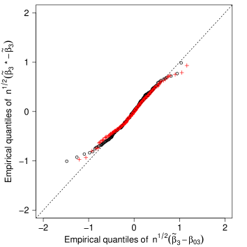
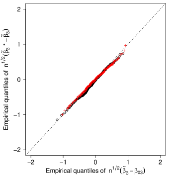
(c)	(d)

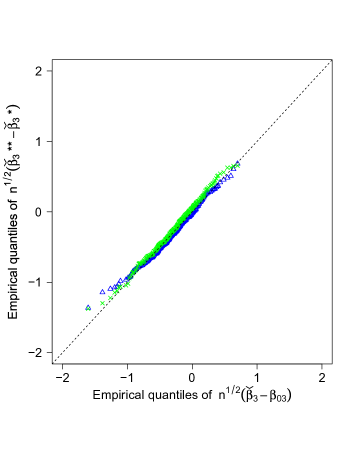
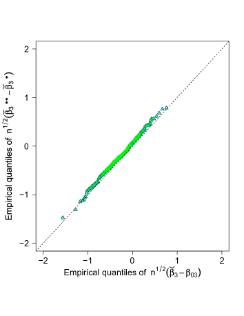
Figure 1: QQ plots for the New AL1 ( ), New AL2 ( +), New L1 ( ), and New L2 ( $\times$) methods for estimating $\beta_{3}=$0$\cdot$25 when $n=250$. (a) and (b) adaptive $L_{1}$ method when $\tau=$0$\cdot$5 and $\tau=$0$\cdot$7, respectively; (c) and (d) $L_{1}$ method when $\tau=$0$\cdot$5 and $\tau=$0$\cdot$7, respectively.

Figure 1 displays the QQ plots of the quantiles of the wild residual bootstrapped estimator versus the empirical quantiles of the corresponding penalized estimator for estimating the smallest coefficient $\beta_{3}=$0$\cdot$25 for both the $L_{1}$ penalty and the adaptive $L_{1}$ penalty when sample size $n=250$ and $400$, for $\tau=$0$\cdot$5 and 0$\cdot$7, respectively. Overall, the wild residual bootstrapped distribution has satisfactory performance.

Table 3: Empirical coverage probabilities ($\times 100$) and average interval lengths (in parentheses) for nominal 95% confidence intervals

	$\beta_{1}=\Phi^{-1}(\tau)$	$\beta_{3}=$ 0$\cdot$25	$\beta_{5}=$ 0$\cdot$5	$\beta_{7}=1$	$\beta_{9}=2$	Zeros	TP	FP
			$\tau=$0$\cdot$5	$n=250$
New AL1	92$\cdot$4 (0$\cdot$22)	94$\cdot$8 (0$\cdot$09)	93$\cdot$3 (0$\cdot$09)	94$\cdot$9 (0$\cdot$07)	94$\cdot$0 (0$\cdot$08)	99$\cdot$0 (0$\cdot$03)	4	0$\cdot$2
New AL2	91$\cdot$4 (0$\cdot$28)	94$\cdot$3 (0$\cdot$09)	93$\cdot$5 (0$\cdot$09)	93$\cdot$9 (0$\cdot$07)	93$\cdot$8 (0$\cdot$08)	99$\cdot$2 (0$\cdot$03)	4	0$\cdot$2
New L1	93$\cdot$6 (0$\cdot$14)	93$\cdot$9 (0$\cdot$10)	93$\cdot$0 (0$\cdot$09)	95$\cdot$3 (0$\cdot$08)	94$\cdot$3 (0$\cdot$09)	95$\cdot$1 (0$\cdot$05)	4	2$\cdot$8
New L2	92$\cdot$6 (0$\cdot$15)	94$\cdot$4 (0$\cdot$10)	92$\cdot$9 (0$\cdot$09)	95$\cdot$4 (0$\cdot$08)	94$\cdot$5 (0$\cdot$09)	95$\cdot$0 (0$\cdot$05)	4	2$\cdot$8
Full RS	93$\cdot$9 (0$\cdot$37)	97$\cdot$0 (0$\cdot$12)	95$\cdot$2 (0$\cdot$11)	96$\cdot$5 (0$\cdot$09)	96$\cdot$1 (0$\cdot$11)	96$\cdot$7 (0$\cdot$10)	4	6
Full WB	91$\cdot$5 (0$\cdot$35)	97$\cdot$0 (0$\cdot$11)	96$\cdot$2 (0$\cdot$11)	97$\cdot$2 (0$\cdot$09)	96$\cdot$2 (0$\cdot$10)	96$\cdot$7 (0$\cdot$10)	4	6
TS AL RS	95$\cdot$1 (0$\cdot$34)	97$\cdot$6 (0$\cdot$14)	97$\cdot$5 (0$\cdot$11)	97$\cdot$1 (0$\cdot$13)	98$\cdot$4 (0$\cdot$15)	99$\cdot$3 (0$\cdot$11)	4	0$\cdot$2
TS AL WB	93$\cdot$2 (0$\cdot$32)	93$\cdot$6 (0$\cdot$11)	95$\cdot$8 (0$\cdot$09)	95$\cdot$4 (0$\cdot$10)	97$\cdot$2 (0$\cdot$10)	99$\cdot$1 (0$\cdot$09)	4	0$\cdot$2
TS L RS	94$\cdot$7 (0$\cdot$33)	96$\cdot$7 (0$\cdot$13)	96$\cdot$8 (0$\cdot$12)	97$\cdot$5 (0$\cdot$12)	97$\cdot$8 (0$\cdot$14)	96$\cdot$9 (0$\cdot$12)	4	2$\cdot$8
TS L WB	93$\cdot$2 (0$\cdot$32)	93$\cdot$8 (0$\cdot$11)	94$\cdot$8 (0$\cdot$10)	96$\cdot$0 (0$\cdot$10)	96$\cdot$3 (0$\cdot$11)	96$\cdot$6 (0$\cdot$10)	4	2$\cdot$8
Oracle RS	-	98$\cdot$6 (0$\cdot$14)	96$\cdot$2 (0$\cdot$12)	98$\cdot$4 (0$\cdot$11)	97$\cdot$9 (0$\cdot$13)	-	4	0
Oracle WB	-	96$\cdot$4 (0$\cdot$10)	95$\cdot$0 (0$\cdot$10)	96$\cdot$1 (0$\cdot$08)	95$\cdot$7 (0$\cdot$09)	-	4	0
			$\tau=$0$\cdot$7	$n=400$
New AL1	91$\cdot$6 (0$\cdot$27)	93$\cdot$6 (0$\cdot$07)	94$\cdot$7 (0$\cdot$06)	93$\cdot$5 (0$\cdot$07)	93$\cdot$8 (0$\cdot$07)	98$\cdot$9 (0$\cdot$03)	5	0$\cdot$1
New AL2	91$\cdot$6 (0$\cdot$27)	93$\cdot$8 (0$\cdot$07)	94$\cdot$8 (0$\cdot$06)	93$\cdot$6 (0$\cdot$07)	94$\cdot$3 (0$\cdot$07)	99$\cdot$2 (0$\cdot$04)	5	0$\cdot$0
New L1	92$\cdot$5 (0$\cdot$27)	93$\cdot$8 (0$\cdot$08)	95$\cdot$2 (0$\cdot$07)	94$\cdot$7 (0$\cdot$08)	93$\cdot$9 (0$\cdot$07)	95$\cdot$6 (0$\cdot$04)	5	2$\cdot$1
New L2	92$\cdot$8 (0$\cdot$27)	94$\cdot$0 (0$\cdot$08)	95$\cdot$6 (0$\cdot$07)	94$\cdot$6 (0$\cdot$08)	94$\cdot$0 (0$\cdot$07)	96$\cdot$1 (0$\cdot$04)	5	2$\cdot$1
Full RS	95$\cdot$6 (0$\cdot$30)	96$\cdot$1 (0$\cdot$09)	95$\cdot$1 (0$\cdot$08)	95$\cdot$8 (0$\cdot$09)	96$\cdot$1 (0$\cdot$08)	96$\cdot$0 (0$\cdot$08)	5	5
Full WB	93$\cdot$1 (0$\cdot$29)	95$\cdot$6 (0$\cdot$09)	96$\cdot$1 (0$\cdot$08)	95$\cdot$2 (0$\cdot$08)	95$\cdot$4 (0$\cdot$08)	95$\cdot$9 (0$\cdot$08)	5	5
TS AL RS	95$\cdot$3 (0$\cdot$30)	96$\cdot$3 (0$\cdot$07)	96$\cdot$1 (0$\cdot$08)	95$\cdot$4 (0$\cdot$08)	94$\cdot$5 (0$\cdot$08)	99$\cdot$3 (0$\cdot$09)	5	0$\cdot$1
TS AL WB	92$\cdot$7 (0$\cdot$28)	96$\cdot$6 (0$\cdot$07)	96$\cdot$9 (0$\cdot$07)	96$\cdot$1 (0$\cdot$08)	95$\cdot$5 (0$\cdot$08)	99$\cdot$2 (0$\cdot$08)	5	0$\cdot$1
TS L RS	94$\cdot$8 (0$\cdot$30)	96$\cdot$0 (0$\cdot$08)	95$\cdot$4 (0$\cdot$08)	95$\cdot$5 (0$\cdot$08)	95$\cdot$0 (0$\cdot$08)	95$\cdot$5 (0$\cdot$08)	5	2$\cdot$1
TS L WB	92$\cdot$4 (0$\cdot$28)	96$\cdot$4 (0$\cdot$07)	96$\cdot$7 (0$\cdot$08)	95$\cdot$2 (0$\cdot$08)	95$\cdot$6 (0$\cdot$08)	96$\cdot$0 (0$\cdot$08)	5	2$\cdot$1
Oracle RS	95$\cdot$6 (0$\cdot$30)	96$\cdot$3 (0$\cdot$08)	95$\cdot$6 (0$\cdot$07)	95$\cdot$9 (0$\cdot$08)	95$\cdot$9 (0$\cdot$08)	-	5	0
Oracle WB	92$\cdot$8 (0$\cdot$28)	95$\cdot$8 (0$\cdot$08)	96$\cdot$8 (0$\cdot$07)	95$\cdot$7 (0$\cdot$08)	95$\cdot$4 (0$\cdot$07)	-	5	0

• New AL1: adaptive $L_{1}$ method with wild residual bootstrap ($\gamma=1$); New AL2: adaptive $L_{1}$ method with wild residual bootstrap ($\gamma=2$); New L1: $L_{1}$ method with modified wild residual bootstrap (data-driven choice of $a_{n}$); New L2: $L_{1}$ method with modified wild residual bootstrap ($a_{n}=n^{-1/3}$); Full RS: full model with rank-score method; Full WB: full model with wild residual bootstrap; TS AL RS: two-step procedure, adaptive $L_{1}$ ($\gamma=1$) followed by rank-score method for the refitted model; TS AL WB: two-step procedure, adaptive $L_{1}$ ($\gamma=1$) followed by wild residual bootstrap for the refitted model; TS L RS: two-step procedure, lasso followed by rank-score method for the refitted model; TS L WB: two-step procedure, lasso followed by wild residual bootstrap for the refitted model; Oracle RS: oracle model with rank-score method; Oracle WB: oracle model with wild residual bootstrap; Zeros: the reported average coverage probability (length) is the average for all zero coefficients; TP: average number of true positives; FP: average number of false positives.

References

- Boyd and Vandenberghe, (2004) Boyd, S. and Vandenberghe, L. (2004). Convex Optimization. Cambridge: Cambridge University Press.
- Buchholz et al., (2008) Buchholz, A., Holländer, N., and Sauerbrei, W. (2008). On properties of predictors derived with a two-step bootstrap model averaging approach – A simulation study in the linear regression model. Computational Statistics & Data Analysis, 52(5):2778–2793.
- Camponovo, (2015) Camponovo, L. (2015). On the validity of the pairs bootstrap for lasso estimators. Biometrika, 102(4):981–987.
- Chatterjee and Lahiri, (2010) Chatterjee, A. and Lahiri, S. (2010). Asymptotic properties of the residual bootstrap for lasso estimators. Proceedings of the American Mathematical Society, 138(12):4497–4509.
- Chatterjee and Lahiri, (2013) Chatterjee, A. and Lahiri, S. (2013). Rates of convergence of the adaptive lasso estimators to the oracle distribution and higher order refinements by the bootstrap. The Annals of Statistics, 41(3):1232–1259.
- Chatterjee and Lahiri, (2011) Chatterjee, A. and Lahiri, S. N. (2011). Bootstrapping lasso estimators. Journal of the American Statistical Association, 106(494):608–625.
- Cheng and Huang, (2010) Cheng, G. and Huang, J. Z. (2010). Bootstrap consistency for general semiparametric M-estimation. The Annals of Statistics, 38(5):2884–2915.
- De Bin et al., (2015) De Bin, R., Janitza, S., Sauerbrei, W., and Boulesteix, A.-L. (2015). Subsampling versus bootstrapping in resampling-based model selection for multivariable regression. Biometrics, 72:272–280.
- Feng et al., (2011) Feng, X., He, X., and Hu, J. (2011). Wild bootstrap for quantile regression. Biometrika, 98(4):995–999.
- Ihorst et al., (2004) Ihorst, G., Frischer, T., Horak, F., Schumacher, M., Kopp, M., Forster, J., Mattes, J., and Kuehr, J. (2004). Long-and medium-term ozone effects on lung growth including a broad spectrum of exposure. European Respiratory Journal, 23(2):292–299.
- Knight, (1998) Knight, K. (1998). Limiting distributions for regression estimators under general conditions. The Annals of Statistics, 26(2):755–770.
- Koenker, (2005) Koenker, R. (2005). Quantile Regression. Cambridge: Cambridge University Press.
- Koenker, (2016) Koenker, R. (2016). quantreg: Quantile regression. r package version 5.35.
- Koenker and Bassett, (1978) Koenker, R. and Bassett, G. (1978). Regression quantiles. Econometrica, 46:33–50.
- Koenker et al., (2017) Koenker, R., Chernozhukov, V., He, X., and Peng, L., editors (2017). Handbook of Quantile Regression. Chapman & Hall/CRC.
- Lee et al., (2014) Lee, E. R., Noh, H., and Park, B. U. (2014). Model selection via Bayesian information criterion for quantile regression models. Journal of the American Statistical Association, 109(505):216–229.
- Leeb and Pötscher, (2008) Leeb, H. and Pötscher, B. M. (2008). Sparse estimators and the oracle property, or the return of Hodges’ estimator. Journal of Econometrics, 142(1):201–211.
- Minnier et al., (2011) Minnier, J., Tian, L., and Cai, T. (2011). A perturbation method for inference on regularized regression estimates. Journal of the American Statistical Association, 106(496):1371–1382.
- Pötscher and Schneider, (2009) Pötscher, B. M. and Schneider, U. (2009). On the distribution of the adaptive lasso estimator. Journal of Statistical Planning and Inference, 139(8):2775–2790.
- van der Vaart, (1998) van der Vaart, A. W. (1998). Asymptotic Statistics. Cambridge University Press.
- van der Vaart and Wellner, (1996) van der Vaart, A. W. and Wellner, J. A. (1996). Weak Convergence and Empirical Processes. New York: Springer.
- Wang et al., (2012) Wang, L., Wu, Y., and Li, R. (2012). Quantile regression for analyzing heterogeneity in ultra-high dimension. Journal of the American Statistical Association, 107(497):214–222.
- Wu and Liu, (2009) Wu, Y. and Liu, Y. (2009). Variable selection in quantile regression. Statistica Sinica, 19:801–817.
- Zou, (2006) Zou, H. (2006). The adaptive lasso and its oracle properties. Journal of the American Statistical Association, 101(476):1418–1429.
- Zou and Yuan, (2008) Zou, H. and Yuan, M. (2008). Composite quantile regression and the oracle model selection theory. The Annals of Statistics, 36:1108–1126.