Exact minimum number of bits
to stabilize a linear system

Abstract

We consider an unstable scalar linear stochastic system, $X_{n+1}=aX_{n}+Z_{n}-U_{n}$, where $a\geq 1$ is the system gain, $Z_{n}$’s are independent random variables with bounded $\alpha$-th moments, and $U_{n}$’s are the control actions that are chosen by a controller who receives a single element of a finite set $\{1,\ldots,M\}$ as its only information about system state $X_{i}$. We show new proofs that $M>a$ is necessary and sufficient for $\beta$-moment stability, for any $\beta<\alpha$. Our achievable scheme is a uniform quantizer of the zoom-in / zoom-out type that codes over multiple time instants for data rate efficiency; the controller uses its memory of the past to correctly interpret the received bits. We analyze its performance using probabilistic arguments. We show a simple proof of a matching converse using information-theoretic techniques. Our results generalize to vector systems, to systems with dependent Gaussian noise, and to the scenario in which a small fraction of transmitted messages is lost.

I Introduction

We study the tradeoff between stabilizability of a linear stochastic system and the coarseness of the quantizer used to represent the state. The evolution of the system is described by

$$X_{n+1}=aX_{n}+Z_{n}-U_{n},$$ (1)

where constant $a\geq 1$; $X_{1}$ and $Z_{1},Z_{2},\ldots$ are independent random variables with bounded $\alpha$-th moments, and $U_{n}$ is the control action chosen based on the history of quantized observations. More precisely, an $M$-bin causal quantizer-controller for $X_{1},X_{2},\ldots$ is a sequence $\{\mathsf{f}_{n},\mathsf{g}_{n}\}_{n=1}^{\infty}$, where $\mathsf{f}_{n}\colon\mathbb{R}^{n}\mapsto[M]$ is the encoding (quantizing) function, and $\mathsf{g}_{n}\colon[M]\mapsto\mathbb{R}^{n}$ is the decoding (controlling) function, and $[M]\triangleq\{1,2,\ldots,M\}$. At time $i$, the controller outputs

$$U_{n}=\mathsf{g}_{n}(\mathsf{f}_{1}(X_{1}),\mathsf{f}_{2}(X^{2}),\ldots,\mathsf{f}_{n}(X^{n})).$$ (2)

The fundamental operational limit of quantized control of interest in this paper is the minimum number of quantization bins to achieve $\beta$-moment stability:

$$M^{\star}_{\beta}\triangleq\min\bigg{\{}M\colon \exists\,M\text{-bin causal quantizer-controller }$$

$$\text{ s.t.~{} }\lim\sup_{n}\mathbb{E}\left[|X_{n}|^{\beta}\right]<\infty\bigg{\}},$$ (3)

where $0<\beta<\alpha$ is fixed.

The main results of the paper are new proofs of the following achievability and converse theorems, whose various special cases have been previously shown in literature.

Theorem 1 (achievability).

Let $X_{1},~{}Z_{n}$ in (1) be independent random variables with bounded $\alpha$-moments. Then for any $0<\beta<\alpha$

$$M^{\star}_{\beta}\leq\lfloor a\rfloor+1.$$ (4)

Theorem 2 (converse).

Let $X_{1}$, $Z_{n}$ in (1) be independent random variables. Let $h(X_{1})>-\infty$, where $h(X)\triangleq-\int_{\mathbb{R}}f_{X}(x)\log f_{X}(x)dx$ is the differential entropy. Then, for all $\beta>0$,

$$M^{\star}_{\beta}\geq\lfloor a\rfloor+1.$$ (5)

The first achievability results [1, 2] focused on unstable scalar systems with bounded disturbances, i.e. $|Z_{n}|\leq B$ a.s., and showed that a simple uniform quantizer with the number of quantization bins in (4) stabilizes such systems. That corresponds to the special case $\alpha=\beta=\infty$. Nair and Evans [3] showed that time-invariant fixed-rate quantizers are unable to attain bounded cost if the noise is unbounded [3], regardless of their rate. The reason is that since the noise is unbounded, over time, a large magnitude noise realization will inevitably be encountered, and the dynamic range of the quantizer will be exceeded by a large margin, not permitting recovery. This necessitates the use of adaptive quantizers of zooming type [4, 5, 6]. Such quantizers “zoom out” (i.e. expand their quantization intervals) when the system is far from the target and “zoom in” when the system is close to the target. Nair and Evans [3] constructed such an adaptive fixed-length quantizer with nonuniform quantization levels and showed second-moment stability via a recursive bound on its mean-squared error, under the assumption that the system noise has bounded $2+\epsilon$ moment, for some $\epsilon>0$. Under the same assumption, Yüksel [7] (see [8],[9] for generalizations to vector systems and to $\beta=1,2,\ldots$) showed second-moment stabilizability using a uniform scalar quantizer that enters its zoom-out mode whenever its input falls outside its dynamic range. When applied to encode each $k$-th system state over the following $k$ time instances, the schemes in [3, 7] attain (4) for a large enough $k$. See also [10], which explores the use of constrained quantizers to encode the overflow event over multiple time instances.

The converse in the special case of $\beta=2$ was proved in [3], where it was shown that it is impossible to achieve second moment stability in the system in (1) using a quantizer-controller with the number of bins $<\lfloor a\rfloor+1$. This implies the validity of Theorem 2 for $\beta\geq 2$. Variants of the necessity result in Theorem 2 are known for vector systems with bounded disturbances [11] and model uncertainty [12]; for noiseless vector systems under different stability criteria [13]; for vector linear stochastic systems under second moment constraint stabilized over rate-constrained noiseless [3] and packet-drop [14] channels; for vector linear stochastic systems stabilized in probability over noisy channels [15]; and for nonlinear systems with additive noise stabilized in probability over noisy channels [16, Th. 3.1].

In this paper, we construct a new zoom-in zoom-out scheme that most of the time operates as if the noise were bounded, and relies on a periodic magnitude test to determine whether the state has left the quantized region. Similar to an application of the schemes in [3, 7] to an undersampled system with the transmission of a codeword over multiple time slots mentioned above, our strategy uses coding over multiple time instants, and the controller uses its memory of the past to correctly interpret the received bits. While the controller in the above modification of the known schemes is almost always silent, producing a large signal once in $k$ time instances, our controller is almost always active, producing a control signal optimized for bounded noise. Thus it introduces less delay. If the periodic magnitude test is failed, the quantizer-controller enters the zoom-out mode, which is essentially the same as in [7]: the controller looks for the $X_{n}$ in exponentially larger intervals until it is located, at which point it returns to the zoom-in mode. We provide an elementary analysis of our scheme with an explicit bound on $k$ leading to Theorem 1.

We also present a short proof of the converse result in Theorem 2 that uses information-theoretic arguments. We also provide an elementary converse proof for stabilizability in probability that is tight for non-integer $a$.

In Section II, we describe our achievable scheme and give its analysis. In Section III, we give a proof of the converse in Theorem 2. Our results generalize to constant-length time delays, to control over communication channels that drop a small fraction of packets, to systems with dependent Gaussian noise, and to vector systems. These extensions are presented in Section IV. This is a full version of the conference paper [17]. This paper presents full proofs (the proofs in [17] are either omitted or replaced with proof outlines), and a much more comprehensive discussion of our results and their relationship to past and future research. In addition, Theorem 3, which presents a converse using an elementary probabilistic argument, is not contained in [17].

II Achievable scheme

II-A The idea

Here we explain the idea of our achievable scheme. For readability we focus on the case $a\in[1,2)$ and show that the system can be controlled with 1 bit. In this case we will be able to restrict to two types of tests, a sign test and a magnitude test (see Fig. 1), which simplifies our procedure. The straightforward extension to an arbitrary $a\geq 1$, in which the sign test is replaced by a uniform quantizer, is found in Section II-E below.

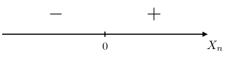
(a) Sign test

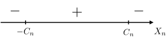
(b) Magnitude test

Figure 1: The binary quantizer uses two kinds of tests on a schedule determined by the previous $\pm$’s to produce the next $+$ or $-$.

In the case of bounded noise a uniform time-invariant quantizer deterministically keeps $X_{n}$ bounded [1, 2]. Indeed, when $|Z_{n}|\leq B$, $n=1,2,\ldots$ and $|X_{1}|\leq C_{1}$, if $C_{1}\geq\frac{B}{1-a/2}$ one can put

$$C_{2}\triangleq(a/2)C_{1}+B\leq C_{1},$$ (6)

and putting further $C_{n+1}\triangleq(a/2)C_{n}+B$, we obtain a monotonically decreasing to $\frac{B}{1-a/2}$ sequence numbers $\{C_{n}\}_{n=1}^{\infty}$. Setting

$$U_{n}=(a/2)C_{n}\mathop{\rm sgn}(X_{n})$$ (7)

requires only 1 bit of knowledge about $X_{n}$ (i.e., its sign). If $|X_{n}|\leq C_{n}$ then

$$|X_{n+1}|\leq(a/2)C_{n}+B=C_{n+1},$$ (8)

and

$$\limsup_{n\to\infty}|X_{n}|\leq\frac{B}{1-a/2}.$$ (9)

Actually, this is the best achievable bound on the uncertainty about the location of $X_{n}$, as a simple volume-division argument shows [11, 18].

When $Z_{n}$ merely have bounded $\alpha$-moments the above does not work because a single large value of $Z_{n}$ will cause the system to explode. However we can use the idea of the bounded case with the following modification. Most of the time, in normal, or zoom-in, mode, the controller assumes the $X_{n}$ are bounded by constants $C_{n}$ and forms the control actions according to the above procedure, but occasionally, on a schedule, the quantizer performs a magnitude test and sends a bit whose sole purpose is to inform the controller whether the $X_{n}$ is staying within desired bounds. If the test is passed, the controller continues in the normal mode, and otherwise, it enters the emergency, or zoom-out, mode, whose purpose is to look for the $X_{n}$ in exponentially larger intervals until it is located, at which point it returns to the zoom-in mode while still occasionally checking for anomalies. We will show that all this can be accomplished with only 1 bit per controller action.

The intuition behind our scheme is the following. At any given time, with high probability $X_{n}$ is not too large. Thus, the emergencies are rare, and when they do occur, the size of the uncertainty region tends to decrease exponentially. The zoom-in mode operates almost exactly as in the bounded case, except that we choose $B$ large enough to diminish the probability that the noise exceeds it. We now proceed to making these intuitions precise in Section II-B.

II-B The Algorithm

Here we describe the algorithm precisely and then prove that it works. Specifically, we consider the setting of Theorem 1 with $a\in[1,2)$ and $Z_{n}$ with bounded $\alpha$-moments. We find $U_{n}$ - a function only of the sequence bits received from the quantizer - that achieves $\beta$-moment stability, for $0<\beta<\alpha$.

First we prepare some constants. We fix $B\geq 1$ large enough. We set the probing factor $P=P(\alpha,\beta)$ - a large positive constant (how large will be explained below, but roughly $P$ blows up as $\beta\uparrow\alpha$). Fix a small $\delta>0$ and a large enough $k=k(a)$ so that

$$(a/2)^{k-1}a \leq 1-3\delta.$$ (10)

We proceed in “rounds” of at least $k+1$ moves, $k$ moves in normal (zoom-in) mode and $k+1$’th move to test whether $X_{n}$ escaped the desired bounds. If that magnitude test comes back normal, the round ends; otherwise the controller enters the emergency (zoom-out) mode, whose duration is variable and which ends once the controller learns a new (larger) bound on $X_{n}$. In normal mode, we use the update rule in (7), where $C_{n}\geq B$ is positive. In the emergency mode, $U_{n}\equiv 0$ while $C_{n}$ grows exponentially. A precise description of the operation of the algorithm is given below.

1. At the start of a round at time-step $m$, $|X_{m}|\leq C_{m}$, the controller is silent, $U_{m}=0$, and $X_{m+1}=aX_{m}+Z_{m}$. Set

   $$C_{m+1}=aC_{m}+B,$$ (11)

   and for each $i\in\{2,\ldots,k\}$,

   $$C_{m+i} =\frac{a}{2}C_{m+i-1}+B$$ (12)

   $$=\left(a/2\right)^{i-1}C_{m+1}+\frac{1-({a}/2)^{i-1}}{1-{a}/2}B.$$ (13)

   In this normal mode operation, the quantizer sends a sequence of signs of $X_{n}$ (see Fig. 1(a)), while the controller applies the controls (7) successively to $X_{m},\ldots,X_{m+k-1}$. This normal mode operation will keep $X_{m+i}$ bounded by $C_{m+i}$ unless some $Z_{m+i}$ is atypically large.

2. The quantizer applies the magnitude test to check whether $|X_{m+k}|\leq C_{m+k}$ (see Fig. 1(b)). If $|X_{m+k}|\leq C_{m+k}$, we return to step 1. If $|X_{m+k}|>C_{m+k}$, this means some $Z_{m+i}$ was abnormally large; the system has blown up and we must do damage control. In this case we enter emergency (zoom-out) mode in Step 3 below.

3. In emergency mode, we repeatedly perform silent ($U_{m+k+j}\equiv 0$) magnitude tests via

   $$C_{m+k+j}=P\,C_{m+k+j-1}=P^{j}C_{m+k}\quad j\geq 0$$ (14)

   until the first time $\tau$ that the magnitude test is passed, i.e.

   $$\tau\triangleq\inf\left\{j\geq 0\colon|X_{m+k+j}|\leq C_{m+k+j}\right\}.$$ (15)

   We then set $m\leftarrow m+k+\tau$ and return to Step 1.

The controller is silent at the start of a round because it does not know the sign of $X_{m}$. Each round thus includes one silent step at the start, and $\tau\geq 0$ silent steps of the emergency mode.

II-C Overview of the Analysis

We analyze the result of each round. At the start of each round $m$ we know that $X_{m}$ is contained within interval $[-C_{m},C_{m}]$. We will show that when $C_{m}$ is large, the uncertainty interval tends to decrease by a constant factor each round.

At the start of the round, $|X_{m}|\leq C_{m}$. Assume that for each $i\in\{0,1,\ldots,k\}$, we have

$$|Z_{m+i}|\leq B.$$ (16)

and thus

$$|X_{m+i}| \leq C_{m+i}.$$ (17)

In particular, applying (10), (11) and (12), we bound the state at the end of the round as

$$|X_{m+k}| \leq C_{m+k}$$ (18)

$$\leq(1-3\delta)\,C_{m}+\frac{B}{1-{a}/2},$$ (19)

which means that $C_{m+k}\leq C_{m}$, provided that $C_{m}\geq\frac{B}{3\delta(1-a/2)}$. Thus, even starting with the silent step we have successfully decreased $C_{m}$, provided that it was large enough.

What if (16) fails to hold? Because the $Z_{i}$ have bounded $\alpha$-moments, by the union bound and Markov’s inequality, the chance (16) fails is at most

$$\mathbb{P}\left[\cup_{i=0}^{k}\left\{{|Z_{m+i}|>B}\right\}\right]\leq(k+1)\,\mathbb{E}\left[|Z|^{\alpha}\right]B^{-\alpha}.$$ (20)

In this case, we show that we can control the blow-up to avert a catastrophe. Recall that in emergency mode our procedure will take exponentially growing $C_{n}$ (see (14)) so that we will soon observe that $|X_{n}|\leq C_{n}$. The controller then exits emergency mode and returns to the normal mode, starting a new round at time step $n$. Using boundedness of $\alpha$-moments of $Z_{i}$, we will show in Section II-D below that the chance that on step $n=m+k+j$ this fails is exponentially small in $j$. We will see that in each round starting at $X_{m}\in[-C_{m},C_{m}]$, there is a high chance to shrink the magnitude of the state and a small chance to grow larger. In the next section we explain how to obtain precise moment control.

II-D Precise Analysis

Here we give details of the analysis outlined in Section II-C, demonstrating that when the $Z_{n}$ are i.i.d. with bounded $\alpha$-moments, our strategy in Section II-B yields

$$\limsup_{n}\mathbb{E}[|X_{n}|^{\beta}]<\infty$$ (21)

for all $0<\beta<\alpha$.

The following tools will be instrumental in controlling the tails of the accumulated noise.

Proposition 1.

If the random variable $Z$ has finite $\alpha$-moment, then

$$t^{\alpha}\mathbb{P}[|Z|>t]$$ (22)

are bounded in $t$. Conversely, if (22) are bounded in $t$ then $Z$ has a finite $\beta$-moment for any $0<\beta<\alpha$.

Proof.

The first part is the Markov inequality. The second is a standard use of the tail-sum formula. ∎

Lemma 1.

Suppose $a>1$ is fixed and $Z_{i}$ are (arbitrarily coupled) random variables with uniformly bounded absolute $\alpha$ moments. Then the random variables

$$\tilde{Z}_{j}\triangleq\sum_{i=0}^{j}a^{-i}Z_{i}$$ (23)

also have uniformly bounded absolute $\alpha$-moments.

Proof.

It is easy to see that for any $\alpha>0,~{}\varepsilon>0$ there is $c=c_{\alpha,\varepsilon}$ such that for all

$$(x+y)^{\alpha}\leq c_{\alpha,\varepsilon}x^{\alpha}+(1+\varepsilon)y^{\alpha}$$ (24)

holds for all $x,y\geq 0$. Indeed, to see this, assume without loss of generality that $x=1$, and note that when $y$ is sufficiently large we already have

$$(1+y)^{\alpha}\leq(1+\varepsilon)y^{\alpha}.$$ (25)

The set of $y$ for which (25) does not hold is bounded, hence so is the value of $(1+y)^{\alpha}$; take $c$ to be an upper bound for this expression. The equation will now hold for any value of $y$.

Applying (24) repeatedly yields

$$|\tilde{Z}_{k}|^{\alpha} \leq$$ (26)

$$c|Z_{0}|^{\alpha}+c\sum_{i=1}^{k-1}(1+\epsilon)^{i}a^{-\alpha i}|Z_{i}|^{\alpha}+(1+\varepsilon)^{k}a^{-\alpha k}|Z_{k}|^{\alpha}.$$

Since $\mathbb{E}\left[|Z_{i}|^{\alpha}\right]$ are uniformly bounded and for $1+\varepsilon<a^{\alpha}$ the geometric series $\sum_{i=1}^{j-1}(1+\epsilon)^{i}a^{-\alpha i}$ converges, $\mathbb{E}[|\tilde{Z}_{j}|^{\alpha}]$ is bounded uniformly in $j$, as desired. ∎

Remark 1.

The mild assumptions of Lemma 1 will make it easy to generalize our results to dependent noise in Section IV-C below.

The bound in Lemma 2 below considers the evolution of the system over $k+1+\tau$ steps, where $\tau$ (15) determines the end of the round. Note that $\tau$ is a stopping time of the filtration generated by $\{X_{n}\}$.

Lemma 2.

Fix $B,P>0$ and consider our algorithm described in Section II-B with these parameters. Suppose that time-step $m$ is the start of a round, so that the round ends on time-step $m+k+\tau$. For all $1<a<2$ and for all $0\leq j\leq\tau$, it holds that

$$~{}\max\left\{|X_{m+1}|,\ldots,|X_{m+k+j}|,C_{m+k+j}\right\}$$ (27)

$$\leq ~{}Pa^{k+j}\left(2C_{m}+\frac{a\,B}{(2-a)(a-1)}+\sum_{\ell=0}^{k+j-1}a^{-\ell-1}|Z_{m+\ell}|\right),$$

Proof.

Appendix. ∎

Proof of Theorem 1 for the case $a\in[1,2)$.

To avoid a special treatment of the case $a=1$, we assume that $a>1$. This is without loss because showing stability for $a$ implies stability for all $a^{\prime}\leq a$. First we prepare some constants. Recall the choices of $k$ and $\delta$ in (10).

• Fix $\Delta<\alpha-\beta$ an arbitrary fixed constant, e.g. $\Delta=\frac{\alpha-\beta}{3}$, so that

  $$\beta=\alpha-3\Delta.$$ (28)

• Fix $P$ large enough so that

  $$P/a\geq\max\left\{\left(\frac{a}{1-\delta}\right)^{\alpha-\Delta},~{}2^{k},~{}\frac{a^{k+1}}{2(a-1)}\right\}.$$ (29)

Suppose that time-step $m$ is the start of a round, so that the round ends on time-step $m+k+\tau$, with stopping time $\tau=0$ usually.

We define a modified sequence $\tilde{X}_{n}$ through, for $1\leq i\leq k+\tau$,

$$\tilde{X}_{m+i}\triangleq ~{}\left(\frac{1}{1-\delta}\right)^{\tau-|i-k|_{+}}$$ (30)

$$~{}\max\left\{|X_{m+k}|,\ldots,|X_{m+k+\tau}|,C_{m+k+\tau}\right\},$$

where $|\cdot|_{+}\triangleq\max\{0,\cdot\}$. Clearly this definition ensures that

$$|X_{m+k+j}|\leq\tilde{X}_{m+k+j}\quad 0\leq j\leq\tau.$$ (31)

Furthermore, for all $1\leq i\leq k-1$, there exists universal constants $K_{1},K_{2},K_{3}$ that depend on $a$, $k$ and $B$ such that (Appendix -A)

$$\mathbb{E}\left[|X_{m+i}|^{\beta}\right]\leq K_{1}\,\mathbb{E}\left[\tilde{X}_{m+k}^{\beta}\right]+K_{2}\,\mathbb{E}\left[\tilde{X}_{m}^{\beta}\right]+K_{3}.$$ (32)

Inequalities (31) and (32) together mean that to establish (21), it is sufficient to prove

$$\limsup_{n}\mathbb{E}[\tilde{X}_{n}^{\beta}]<\infty.$$ (33)

The rest of the proof is focused in establishing (33).

By definition (30),

$$\tilde{X}_{m+i}\leq\tilde{X}_{m+1}\quad i=2,\ldots,k+\tau,$$ (34)

with equality for $i\leq k$.

We will show that

$$\mathbb{E}[\tilde{X}_{m+1}^{\beta}] \leq(1-\delta)^{\beta}\mathbb{E}[\tilde{X}_{m}^{\beta}]+K,$$ (35)

where $K=K(P,k,\delta)$ is a constant that may depend on $P,k,\delta$ (but is independent of $m$). Together, inequalities (34) and (35) ensure that $\limsup_{n}\mathbb{E}[\tilde{X}_{n}^{\beta}]$ is bounded above by $\frac{K}{1-(1-\delta)^{\beta}}$.

The intuition behind the definition for $\tilde{X}_{n}$ is as follows. We want to construct a dominating sequence $\tilde{X}_{n}$ with the expected decrease property in (35). During emergency mode, the original sequence $X_{n}$ may increase on average during rounds. The sequence $\tilde{X}_{n}$ in (30) takes the potential increase during each round up front, achieving the desired expected decrease property. We will see that $P$ in (29) is chosen so that the constant-factor decrease of the system is preserved when switching between rounds.

To show (35), we define the filtration $\mathcal{F}_{n}$ as follows: $\mathcal{F}_{n}$ is the $\sigma$-algebra generated by the sequences $Z_{1},Z_{2},\ldots,Z_{n-1}$ and $\tilde{X}_{1},\tilde{X}_{2},\ldots,\tilde{X}_{n}$. Unless $n$ is the end of a round, knowledge of $\tilde{X}_{n}$ involves a peek into the future, so $\mathcal{F}_{n}$ encompasses slightly more information than the naive notion of “information up to time $n$”. The inequality we will show, clearly stronger than (35), is

$$\mathbb{E}[\tilde{X}_{m+1}^{\beta}\mid\mathcal{F}_{m}]\leq(1-\delta)^{\beta}\mathbb{E}[\tilde{X}_{m}^{\beta}\mid\mathcal{F}_{m}]+K.$$ (36)

Define

$$Y_{n}\triangleq\frac{\tilde{X}_{n+1}}{\tilde{X}_{n}+\frac{B}{(1-a/2)(1-3\delta)}}.$$ (37)

We will show (36) by the means of the following two statements, where $m$ is the transition between rounds:

1. For sufficiently large $k$ and $P$ in (10) and (29), respectively, it holds that

   $$\mathbb{P}\left[Y_{m}\geq t|\mathcal{F}_{m}\right]=O\left(t^{-(\alpha-\Delta)}\right),$$ (38)

2. As $B\to\infty$,

   $$\mathbb{P}\left[Y_{m}\leq 1-3\delta\mid\mathcal{F}_{m}\right]\to 1.$$ (39)

We use (38) and (39) to show (36) as follows. First, observe that by (38) and Proposition 1, $\{Y_{m}|\mathcal{F}_{m}\}$ has bounded $\beta+\Delta$ - moment since we assumed (28) when choosing $\Delta$. Furthermore, since the right side of (38) is independent of $\mathcal{F}_{m}$, the $\beta+\Delta$ - moment of $Y_{m}$ is bounded uniformly in $m$. Now, pick $p>1$ so that $\beta p\leq\beta+\Delta$, and let $q$ satisfy $\frac{1}{p}+\frac{1}{q}=1$. Write

$$~{}\mathbb{E}\left[Y_{m}^{\beta}\mid\mathcal{F}_{m}\right]$$

$$\leq ~{}(1-3\delta)^{\beta}+\mathbb{E}\left[Y_{m}^{\beta}\,1\left\{Y_{m}>1-3\delta\right\}\mid\mathcal{F}_{m}\right]$$ (40)

$$\leq ~{}(1-3\delta)^{\beta}+\left(\mathbb{E}\left[Y_{m}^{\beta p}\mid\mathcal{F}_{m}\right]\right)^{\frac{1}{p}}\left(\mathbb{P}\left[Y_{m}>1-3\delta\mid\mathcal{F}_{m}\right]\right)^{\frac{1}{q}}$$ (41)

$$\to ~{}(1-3\delta)^{\beta},\quad B\to\infty,$$ (42)

where (41) is by Hölder’s inequality, and the second term in (41) vanishes as $B\to\infty$ due to (39) and uniform boundedness of the $\beta+\Delta$ - moment of $\{Y_{m}\mid\mathcal{F}_{m}\}$. Note that convergence in (42) is uniform in $m$. It follows that for a large enough $B$ (how large depends on the values of $P,k,\delta$),

$$\mathbb{E}\left[Y_{m}^{\beta}\mid\mathcal{F}_{m}\right]\leq(1-2\delta)^{\beta}.$$ (43)

Rewriting (43) using (37) yields

$$\mathbb{E}[\tilde{X}_{m+1}^{\beta}\mid\mathcal{F}_{m}] \leq(1-2\delta)^{\beta}\left(\tilde{X}_{m}+\frac{B}{(1-a/2)(1-3\delta)}\right)^{\beta}$$ (44)

$$\leq(1-\delta)^{\beta}\tilde{X}_{m}^{\beta}+K,$$ (45)

where to write (45) we used (24). This establishes the inequality (36).

To complete the proof of Theorem 1, it remains to establish (38) and (39).

To show (38), recall that the round ends at stopping time $m+k+\tau$. Since the events $\{\tau=j\}$ are disjoint, we have

$$\mathbb{P}\left[Y_{m}\geq t|\mathcal{F}_{m}\right] =\sum_{j=0}^{\infty}\mathbb{P}[Y_{m}\geq t,\tau=j|\mathcal{F}_{m}]$$

$$\phantom{=}+\mathbb{P}[Y_{m}\geq t,\tau=\infty|\mathcal{F}_{m}]$$ (46)

Note that since $m$ is the end of the previous round, $\mathcal{F}_{m}$ does not contain any information about the future.

We estimate the probability of the event in $\mathbb{P}[Y_{m}\geq t,\tau=j|\mathcal{F}_{m}]$ in two ways, and use the better estimate on each term individually.

We express the system state at time $m+i$ in terms of the system state at time $m$:

$$X_{m+i} =a^{i}\left(X_{m}+\sum_{\ell=0}^{i-1}a^{-\ell-1}U_{m+\ell}+\sum_{\ell=0}^{i-1}a^{-\ell-1}Z_{m+\ell}\right).$$ (47)

Using (7), (11), (12) and recalling that $U_{m}=0$, we can crudely bound the cumulative effect of controls on $X_{m+i}$ as

$$a^{i}\left|\sum_{\ell=0}^{k-1}a^{-\ell-1}U_{m+\ell}\right| \leq a^{i}\left(a/2\right)\sum_{\ell=1}^{\infty}a^{-\ell-1}$$ (48)

$$\phantom{=}\left(\left(a/2\right)^{\ell-1}C_{m+1}+\frac{1-({a}/2)^{\ell-1}}{1-{a}/2}B\right)$$

$$=a^{i}\left(C_{m}+\frac{B}{a-1}\right).$$ (49)

Recalling the definitions of $\tilde{X}_{n}$, $Y_{n}$ in (30), (37), respectively, and invoking Lemma 2, we see that if $\{Y_{m}\geq t,\tau=j\}$ holds, then

$$~{}t(1-\delta)^{k+j-1}\left(\tilde{X}_{m}+\frac{B}{(1-a/2)(1-3\delta)}\right)$$ (50)

$$\leq ~{}Pa^{k+j}\left(2C_{m}+\frac{aB}{(2-a)(a-1)}+\sum_{\ell=0}^{k+j-1}a^{-\ell-1}|Z_{m+\ell}|\right).$$

Noting that both $C_{m}$ and $\frac{aB}{2-a}$ are dominated by $\tilde{X}_{m}+\frac{B}{(1-a/2)(1-3\delta)}\geq 1$, we can weaken (50) as

$$\!\!\!t(1-\delta)^{k+j-1}\leq Pa^{k+j}\left(2+\frac{1}{a-1}+\sum_{\ell=0}^{k+j-1}a^{-\ell-1}|Z_{m+\ell}|\right).$$ (51)

Applying Lemma 1 and Proposition 1, we deduce that the probability of the event in (51) is

$$O\left(\left(\frac{a}{1-\delta}\right)^{\alpha j}t^{-\alpha}\right).$$ (52)

The bound in (52) works well for small $j$ / large $t$. For large $j$ / small $t$, we observe that $\{Y_{m}\geq t,\tau=j\}\subseteq\{\tau\geq j\}$ and apply the following reasoning. The event $\{\tau\geq j\}$ means that the emergency did not end at time $j$; in other words,

$$|X_{m+k+j-1}| >C_{m+k+j-1}$$ (53)

$$=P^{j}\left(2\left(a/2\right)^{k}C_{m}+\frac{B}{1-{a}/2}\right),$$ (54)

where to write (54) we used (11), (13), and (14). Substituting $i\leftarrow k+j$ into (47) and recalling (49) and $|X_{m}|\leq C_{m}$, we weaken (53)–(54) as

$$\phantom{=}a^{k+j}\bigg{(}2C_{m}+\frac{aB}{(2-a)(a-1)}+\sum_{\ell=0}^{k+j-1}a^{-\ell-1}|Z_{m+\ell}|\bigg{)}$$

$$>P^{j}\left(2\left(a/2\right)^{k}C_{m}+\frac{B}{1-{a}/2}\right),$$ (55)

the event equivalent to

$$(a/P)^{j}\sum_{\ell=0}^{k+j-1}a^{-\ell-1}|Z_{m+\ell}|\geq 2\left((1/2)^{k}-(a/P)^{j}\right)C_{m}$$

$$+\left((1/a)^{k}-\frac{a(a/P)^{j}}{2(a-1)}\right)\frac{B}{1-a/2}.$$ (56)

Due to the choice of $P$ in (29), the coefficients in front of $C_{m}$ and $B$ in the right side of (56) are nonnegative for all $j\geq 1$. Bounding the probability of the event in (56) using Lemma 1 and Proposition 1, we conclude that

$$\mathbb{P}\left[\tau\geq j\right]=O\left(\left(P/a\right)^{-j\alpha}\right).$$ (57)

Furthermore, (57) means that $\mathbb{P}\left[\tau=\infty\right]=0$. Indeed, $1\{\tau=\infty\}=\prod_{j=0}^{\infty}1\left\{\tau\geq j\right\}=\lim_{j\to\infty}1\left\{\tau\geq j\right\}$ and by Fatou’s lemma,

$$\mathbb{P}\left[\tau=\infty\right]\leq\lim_{j\to\infty}\mathbb{P}\left[\tau\geq j\right]=0,$$ (58)

thus the corresponding term can be eliminated from (46).

Juxtaposing (52) and (57), we conclude that the probability $\mathbb{P}[Y_{m}\geq t,\tau=j|\mathcal{F}_{m}]$ is bounded by

$$O\left(\min\left\{\left(\frac{a}{1-\delta}\right)^{\alpha j}t^{-\alpha},\left(P/a\right)^{-j\alpha}\right\}\right).$$ (59)

Since (29) ensures that $(P/a)^{\Delta}\geq\left(\frac{a}{1-\delta}\right)^{\alpha}$, we weaken (59) as

$$O\left(\left(P/a\right)^{j\Delta}\min\left\{t^{-\alpha},\left(P/a\right)^{-j\alpha}\right\}\right).$$ (60)

Recall that we have fixed $t$ and are varying $j$; this upper bound peaks at $j$ such that $(P/a)^{j}=t$ at the value $t^{-(\alpha-\Delta)}$ and decays geometrically on each side at rates $(P/a)^{\Delta}$ and $(P/a)^{\alpha-\Delta}$. Hence the sum of all $\mathbb{P}[Y_{m}\geq t,\tau=j|\mathcal{F}_{m}]$ terms in (46) is bounded by the maximum up to a constant factor and therefore (38) holds.

To complete the proof of Theorem 1, it remains to establish (39). By Markov’s inequality (20), with probability converging to $1$ as $B\to\infty$, all terms $Z_{m},\ldots,Z_{m+k}$ are within $[-B,B]$, and $\tau=0$. In such a case, applying (19) and recalling (30), we get

$$\tilde{X}_{m+1} =\max\{|X_{m+k}|,C_{m+k}\}$$ (61)

$$\leq\left(1-3\delta\right)\tilde{X}_{m}+\frac{B}{1-a/2},$$ (62)

which implies that $Y_{m}\leq 1-3\delta$, establishing (39).

∎

II-E Finer Quantization

For $a\geq 2$, the controller receives an element of an $\lfloor a\rfloor+1$-element set instead of a single bit. In this case we restrict our attention to order-statistic tests, meaning that we split the real line into $\lfloor a\rfloor+1$ intervals

$$(-\infty,w_{1,n}),[w_{1,n},w_{2,n}),\dots,[w_{\lfloor a\rfloor,n},\infty),$$ (63)

and the controller receives the index $b_{n}\in\{0,1,\dots,\lfloor a\rfloor\}$ of the interval containing $X_{n}$. The only real issue is for the quantizer and the controller to agree upon a rule for updating the values of $w_{i}$. However, this is easy; in the obvious generalization of our algorithm to higher $a$, the (uniform) quantizer simply breaks up the interval $[-C_{n},\,C_{n}]$ into $\lfloor a\rfloor+1$ equal parts, where $C_{n}$ is the same bound on the state magnitude as before. Both quantizer and controller follow the rules in (12) (with $a/2$ replaced by $a/(\lfloor a\rfloor+1)$ and in (14) to update $C_{n}$. During the normal mode, the controller applies the control

$$U_{n}=-C_{n}+C_{n}\frac{2b_{n}+1}{\lfloor a\rfloor+1}$$ (64)

which reduces to (7) when $\lfloor a\rfloor=1$.

In the case $a<1$, the controller does nothing, which by Lemma 1 achieves $\beta$-moment stability.

III Converse

In this section, we prove the converse result in Theorem 2 using information-theoretic arguments similar to those employed in [3, 20]. Then, we use elementary probability to show an alternative converse result, which implies Theorem 2 unless $a$ is an integer.

Proof of Theorem 2.

Conditional entropy power is defined as

$$N(X|U)\triangleq\frac{1}{2\pi e}\mathop{\rm exp}\left(2h(X|U)\right)$$ (65)

where $h(X|U)=-\int_{\mathbb{R}}f_{X,U}(x,u)\log f_{X|U=u}(x)dx$ is the conditional differential entropy of $X$.

Conditional entropy power is bounded above in terms of moments (e.g. [21, Appendix 2]):

$$N(X) \leq\kappa_{\beta}\mathbb{E}\left[|X|^{\beta}\right]^{\frac{2}{\beta}}$$ (66)

$$\kappa_{\beta} \triangleq\frac{2}{\pi e}\left(e^{\frac{1}{\beta}}\Gamma\left(1+\frac{1}{\beta}\right)\beta^{\frac{1}{\beta}}\right)^{2},$$ (67)

Thus,

$$\kappa_{\beta}\mathbb{E}\left[|X_{n}|^{\beta}\right]^{\frac{2}{\beta}} \geq N\left(X_{n}\right)$$ (68)

$$\geq N\left(X_{n}|U^{n-1}\right),$$ (69)

where (69) holds because conditioning reduces entropy. Next, we show a recursion on $N\left(X_{n}|U^{n-1}\right)$:

$$N\left(X_{n}|U^{n-1}\right) =N(\mathsf{A}X_{n-1}+{Z}_{n-1}|U^{n-1})$$ (70)

$$\geq a^{2}N(X_{n-1}|U^{n-1})+N({Z}_{n-1})$$ (71)

$$\geq a^{2}N(X_{n-1}|U^{n-2})\mathop{\rm exp}\left(-2r\right)+N({Z}_{n-1}),$$ (72)

where (71) is due to the conditional entropy power inequality:

$$N(X+Y|U)\geq N(X|U)+N(Y|U),$$ (73)

which holds as long as $X$ and $Y$ are conditionally independent given $U$, and (72) is obtained by weakening the constraint $|U_{n-1}|\leq M$ to a mutual information constraint $I(X_{n-1};U_{n-1}|U^{n-2})\leq\log M=r$ and observing that

$$\min_{P_{U|X}\colon I(X;U)\leq r}h(X|U) \geq h(X)-r.$$ (74)

It follows from (72) that $r>\log a$ is necessary to keep $N\left(X_{n}|U^{n-1}\right)$ bounded. Due to (69), it is also necessary to keep $\beta$-th moment of $X_{n}$ bounded. ∎

Consider the following notion of stability.

Definition 1.

The system is stabilizable in probability if there exists a control strategy such that for some bounded interval $\mathcal{I}$,

$$\limsup_{n\to\infty}\mathbb{P}\left[X_{n}\in\mathcal{I}\right]>0.$$ (75)

As a simple consequence of Markov’s inequality, if the system is moment-stable, it is also stable in probability. Therefore the following converse for stability in probability implies a converse for moment stability.

Theorem 3.

Assume that $X_{1}$ has a density. To achieve stability in probability, $M\geq\lceil a\rceil$ is necessary.

Proof.

We want to show that for any bounded interval $\mathcal{I}$, if $r<\log a$ then

$$\limsup_{n\to\infty}\mathbb{P}\left[X_{n}\in\mathcal{I}\right]=0.$$ (76)

At first we assume that the density of $X_{1}$ is bounded, that is, $|f_{X_{1}}(x)|\leq f_{\max}$ and that $X_{1}$ is supported on a finite interval, i.e. $|X_{1}|\leq x_{\max}$, for some constants $f_{\max},x_{\max}$.

Since we are showing a converse (impossibility) result, we may relax the operational constraints by revealing the noises $Z_{n},~{}n=1,2,\ldots$ noncausally to both encoder and decoder. Since then the controller can simply subtract the effect of the noise, we may put $Z_{n}\equiv 0$ in (1). Then, $X_{n+1}=a^{n}X_{1}+\tilde{U}_{n}$, where $\tilde{U}_{n}\triangleq\sum_{i=0}^{n}a^{n-i}U_{i}$ is the combined effect of $t$ controls, which can take one of $M^{n}$ values, i.e. $U_{n}=u(m)$ if $X_{1}\in\mathcal{I}_{m}$, $m=1,\ldots,M^{n}$. Regardless of the particular choice of control actions $u(m)$ and quantization intervals $\mathcal{I}_{m}$, for any bounded interval $\mathcal{I}$,

$$\mathbb{P}\left[X_{n+1}\in\mathcal{I}\right] =\mathbb{P}\left[a^{n}X_{1}+\tilde{U}_{n}\in\mathcal{I}\right]$$ (77)

$$=\sum_{m=1}^{M^{n}}\mathbb{P}\left[a^{n}X_{1}+u(m)\in\mathcal{I},X_{1}\in\mathcal{I}_{m}\right]$$ (78)

$$\leq M^{n}a^{-n}f_{\max}|\mathcal{I}|,$$ (79)

and (76) follows for any $M<a$, confirming the necessity of $M\geq\lceil a\rceil$ to achieve weak stability.

Finally, if the density of $X_{1}$ is unbounded, consider the set $\mathcal{S}_{b}\triangleq\left\{x\in\mathbb{R}\colon f_{X_{1}}(x)\leq b\right\}$ and notice that since $1\{f_{X_{1}}(x)>b\}\to 0$ pointwise as $b\to\infty$, by dominated convergence theorem,

$$\mathbb{P}\left[X_{1}\in\mathcal{S}_{b}\right] =\int_{\mathbb{R}}f_{X_{1}}(x)1\{f_{X_{1}}(x)>b\}\mathrm{d}x\to 0\text{ as }b\to\infty.$$ (80)

Therefore for any $\epsilon>0$, one can pick $b>0$ such that $\mathbb{P}\left[X_{1}\in\mathcal{S}_{b}\right]\leq\epsilon$. Then, since we already proved that (76) holds for bounded $f_{X_{1}}$, we conclude

$$\limsup_{n\to\infty}\mathbb{P}\left[X_{n}\in\mathcal{I}\right]\leq\epsilon+\limsup_{n\to\infty}\mathbb{P}\left[X_{n}\in\mathcal{I}|X_{1}\in\mathcal{S}_{b}\right]=\epsilon,$$ (81)

which implies that (76) continues to hold for unbounded $f_{X_{1}}$. ∎

The quantities $\lceil a\rceil$ and $\lfloor a\rfloor+1$ coincide unless $a$ is an integer, thus Theorem 3 shows that for non-integer $a$, the converse (impossibility) part of Theorem 1 continues to hold in the sense of weak stability. Note that the proof of Theorem 3 relaxes the causality requirement. We conjecture that $\lceil a\rceil$ can be replaced by $\lfloor a\rfloor+1$ in its statement, but proving that will require bringing causality back in the picture, and the simple argument in the proof of Theorem 3 will not work.

We conclude Section III with a technical remark.

Remark 2.

The assumptions in Theorem 3 are weaker than those in Theorem 2, because the differential entropy of $X_{1}$ not being $-\infty$ implies that $X_{1}$ must have a density. The assumption that $X_{1}$ must have a density is not superficial. For example, consider $Z_{i}\equiv 0$ and $X_{1}$ uniformly distributed on the Cantor set, and $a=2.9$. Clearly this system can be stabilized with 1 bit, by telling the controller at each step the undeleted third of the interval the state is at. This is lower than the result of Theorem 1, which states that $M^{\star}_{\beta}$ would be $3$ if $X_{1}$ had a density. Beyond distributions with densities, we conjecture that $M^{\star}_{\beta}$ will depend on the Hausdorff dimension of the probability measure of $X_{1}$.

IV Generalizations

In this section, we generalize our results in several directions. In most cases we only outline the mild differences in the proof.

IV-A Constant-Length Time Delays

Many systems have a finite delay in feedback. To model this, we can force $U_{n}$ to depend on only the feedback up to round $n-\ell$, i.e.

$$U_{n}=\mathsf{g}_{n}(\mathsf{f}_{1}(X_{1}),\mathsf{f}_{2}(X^{2}),\ldots,\mathsf{f}_{n-\ell}(X^{n-\ell})),$$ (82)

where $\mathsf{f}_{n}(X^{n})$ is the quantizer’s output at time $n$, as before.

We argue here that this makes no difference in terms of the minimum number of bits required for stability. We state the modified result next.

Theorem 4.

Let $X_{1}$, $Z_{n}$ in (1) be independent random variables with bounded $\alpha$-moments. Assume that $h(X_{1})>-\infty$. The minimum number of quantization points to achieve $\beta$-moment stability, for any $0<\beta<\alpha$ and with any constant delay $\ell$ is given by $\lfloor a\rfloor+1$.

Proof.

The problem here is that the encoder sees the system before the controller can act on it. However, if we also delay the encoder seeing the system by $\ell$ time steps, then we can directly use the algorithm we have already constructed. Specifically, if our artificially delayed sequence of system states is $\{\tilde{X}_{n}\}$, then the real sequence is given by

$$X_{n}=a^{\ell}\tilde{X}_{n}+a^{\ell-1}Z_{n+1}+...+Z_{n+\ell}.$$ (83)

By Theorem 1, we can keep $\mathbb{E}[|\tilde{X}_{n}|^{\beta}]$ bounded for any $\beta<\alpha$ by applying to $\tilde{X}_{n}$ the control in (64) in normal mode and $U_{n}=0$ in the emergency mode. Since with delay, the controller acts on $X_{n}$ rather than on $\tilde{X}_{n}$, we multiply the control action (64) by $a^{\ell}$ to achieve the same effect on $\tilde{X}_{n}$ as without delay. Furthermore, each $Z_{i}$ has bounded $\beta$ moment, so by Lemma 1 their sum will have bounded $\beta$-moment, as desired.

The converse is obvious as even with $\ell=0$, Theorem 2 asserts that the system cannot be stabilized with fewer than $\lfloor a\rfloor+1$ bits.

∎

IV-B Packet drops

Suppose that the encoder cannot send information to the controller at all time-steps. Instead, the encoder can only send information at a deterministic set $\mathcal{T}\subseteq\mathbb{N}$ of times. Formally,

$$U_{n}=\mathsf{g}_{n}(\{\mathsf{f}_{n}(X^{n})\colon n\in\mathcal{T}\}).$$ (84)

As long as the density of $\mathcal{T}$ is high enough on all large, constant-sized scales, the same results go through.

Definition 2.

A set $\mathcal{T}\subseteq\mathbb{N}$ is strongly $p$-dense if there exists $N$ such that for all $n$ we have

$$\frac{|n+i\colon n+i\in\mathcal{T},~{}i=0,\ldots,N-1|}{N}>p.$$ (85)

Note that the constant delay scenario in Section IV-A amounts to control on a strongly $p$-dense set, with $p\in[0,1)$ as close to $1$ as desired.

Theorem 5.

Let $X_{1}$, $Z_{n}$ in (1) be independent random variables with bounded $\alpha$-moments. Assume that $h(X_{1})>-\infty$. The minimum number of quantization points to achieve $\beta$-moment stability is $\lfloor a\rfloor+1$, for any $0<\beta<\alpha$ and on any strongly $p$-dense set with some $p\in[0,1]$ large enough so that

$$\left(\lfloor a\rfloor+1\right)^{p}>a.$$ (86)

Proof.

The requirement (86) ensures that the bounded case works; indeed, it is equivalent to

$$\left(\frac{a}{\lfloor a\rfloor+1}\right)^{p}a^{1-p}<1,$$ (87)

which means that the logarithm of the range of $X_{n}$ decreases on average each time-step.

In the unbounded noise case, we perform the same basic algorithm, but ensuring that the normal mode has enough times in $\mathcal{T}$, so the duration of the normal mode gets longer if $N$ is large. Likewise, in the emergency mode, it will take longer to catch blow-ups. However, a much weaker condition on $\mathcal{T}$ suffices for the emergency mode to end: even if $\mathcal{T}$ contains only $1$ element out of every $N$, we make the probe factor $P$ large enough depending on $N$. The difference between probing every $N$ time steps vs. every time step at most a factor of $a^{N}$ which is a constant. ∎

IV-C Dependent Noise

Here we address a modification in which the noise is correlated rather than independent.

Proposition 2.

Suppose $\{Z_{n}\}$ is a Gaussian process whose covariance matrix ${\mathsf{M}}$ (for any number of samples) has spectrum bounded by $\lambda$. Then there is an independent Gaussian process $\{Z^{\prime}_{n}\}$ such that the random variables $\{Z_{n}+Z^{\prime}_{n}\}$ are i.i.d. Gaussians with variances $\lambda^{2}$.

Proof.

Just make the covariances matrices of $\{Z_{n}\}$ and $\{Z^{\prime}_{n}\}$ add to $\lambda I$; the assumption means both are positive semidefinite, hence define Gaussian processes. ∎

If the rows of ${\mathsf{M}}$ have $\ell^{1}$ norm at most $\lambda$, the assumption of Proposition 2 that ${\mathsf{M}}$ has spectrum bounded by $\lambda$ will be satisfied. Indeed, we can add a positive semidefinite matrix to such an ${\mathsf{M}}$ to obtain a diagonal matrix with each entry at most $\lambda$: if ${\mathsf{M}}$ has an entry of $x$ at positions $(i,j)$ and $(j,i)$ then we add $|x|$ to the $(i,i)$ and $(j,j)$ entries; it is easy to see that the symmetric matrix

$$\begin{pmatrix}|x|&-x\\ -x&|x|\end{pmatrix}$$ (88)

is always positive semidefinite. Therefore doing this for all non-diagonal entries adds a positive semidefinite matrix to ${\mathsf{M}}$ and still results in a spectrum contained in $[0,\lambda]$, meaning ${\mathsf{M}}$ also had spectrum contained in $[0,\lambda]$.

Theorem 6.

The results in Theorems 1, 4, 5 extend to the case when $\{Z_{n}\}$ is correlated Gaussian noise whose covariance matrix has bounded spectrum.

Proof.

As a result of Proposition 2, for any Gaussian noise with known covariance matrix ${\mathsf{M}}$ of bounded spectrum, the controller can simply add extra noise to the system via $U_{n}$ to effectively make the noise i.i.d. Gaussian, reducing this scenario to the i.i.d. case.

∎

IV-D Vector systems

The results generalize to higher dimensional systems

$$X_{n+1}={\mathsf{A}}X_{n}+Z_{n}-\mathsf{B}U_{n},$$ (89)

where ${\mathsf{A}}$ is a $d\times d$ matrix and $Z_{n},~{}U_{n}$ are vectors. The dimensionality of control signals $U_{n}$ can be less than $d$, in which case ${\mathsf{B}}$ is a tall matrix.

For the controls to potentially span the whole space $\mathbb{R}^{d}$ when combined with the multiplication-by-$\mathsf{A}$ amplification, the range of

$$\left[{\mathsf{B}},\,{\mathsf{A}}{\mathsf{B}},\,{\mathsf{A}}^{2}{\mathsf{B}},\,\dots,\,{\mathsf{A}}^{d-1}{\mathsf{B}}\right]$$ (90)

needs to span $\mathbb{R}^{d}$. Such a pair $(\mathsf{A},\mathsf{B})$ of matrices is commonly referred to as controllable. (The $0,\ldots,d-1$ powers of ${\mathsf{A}}$ are sufficient in (90), because by the Cayley-Hamilton theorem any higher power of ${\mathsf{A}}$ is a linear combination of those lower powers). For our results to hold, a weaker condition suffices, namely, we need stabilizability of $({\mathsf{A}},{\mathsf{B}})$, which is to say that only unstable modes need be controllable. More precisely, in the canonical representation of a linear system,

$$\begin{bmatrix}X^{u}_{n+1}\\ X^{s}_{n+1}\end{bmatrix}=\begin{bmatrix}{\mathsf{A}}^{u}&{\mathsf{A}}^{\prime}\\ {\mathsf{0}}&{\mathsf{A}}^{s}\end{bmatrix}\begin{bmatrix}X^{u}_{n}\\ X^{s}_{n}\end{bmatrix}+Z_{n}-\begin{bmatrix}{\mathsf{B}}^{u}\\ {\mathsf{0}}\end{bmatrix}U_{n},$$ (91)

where the matrix ${\mathsf{A}}^{s}$ has all stable eigenvalues, the state coordinates $X^{s}_{n+1}$ cannot be reached by the control $U_{n}$. Stabilizability means that the pair $(\mathsf{A}^{u},\mathsf{B}^{u})$ is controllable, which ensures that unstable modes can be controlled.

The idea behind our generalization to the vector case, previously explored in e.g. [3], is that we can decompose $\mathbb{R}^{d}$ into eigenspaces of ${\mathsf{A}}$ and rotate attention between these parts.

Theorem 7.

Consider the stochastic vector linear system in (89) with $({\mathsf{A}},{\mathsf{B}})$ stabilizable. Let $X_{1},~{}Z_{n}$ be independent random $\mathbb{R}^{d}$-valued random vectors with bounded $\alpha$-moments. Assume that $h(X_{1})>-\infty$. Let $(\lambda_{1},...,\lambda_{d})$ be the eigenvalues of ${\mathsf{A}}$, and set

$$a\triangleq\prod_{j=1}^{d}\max(1,|\lambda_{j}|).$$ (92)

Then for any $0<\beta<\alpha$, the minimum number of quantization points to achieve $\beta$-moment stability is

$$M_{\beta}^{\star}=\lfloor a\rfloor+1.$$ (93)

Proof.

We first consider the case $U_{n}\in\mathbb{R}^{d}$, ${\mathsf{B}}={\mathsf{I}}$:

$$X_{n+1}={\mathsf{A}}X_{n}+Z_{n}-U_{n},$$ (94)

and then explain how to deal with the general stabilizable system in (89).

By using a real Jordan decomposition, we can block-diagonalize ${\mathsf{A}}$ into

$${\mathsf{A}}=\bigoplus_{j}{\mathsf{A}}_{j}$$ (95)

where ${\mathsf{A}}_{j}\colon\mathcal{V}_{j}\to\mathcal{V}_{j}$ with

$$\bigoplus_{j}\mathcal{V}_{j}=\mathbb{R}^{d}$$ (96)

such that:

1. The spectrum of each ${\mathsf{A}}_{j}$ is either a single real $\lambda_{j}$ (possibly with multiplicity) or a pair of complex numbers $\lambda_{j},\bar{\lambda}_{j}$ (with equal multiplicity).

2. The spectral norm of ${\mathsf{A}}_{j}^{k}$ is $|\lambda_{j}|^{k}k^{O(1)}$.

This decomposition splits any vector $X_{n}$ into a sum $X_{n}=\sum_{j}X_{n,j}$. Each $X_{n,j}$ individually satisfies a control equation with matrix ${\mathsf{A}}_{j}$, and we will control these separately. Indeed, if

$$\sup_{n}\mathbb{E}[|X_{n,j}|^{\beta}]<\infty$$ (97)

for all $j$, then we get the desired result. (Note that we do not need to assume that the noise $Z_{n}$ behaves independently on each subspace; getting from separate moment bounds on $X_{n,j}$ to a moment bound on $X_{n}$ does not require any sort of independence.)

If $|\lambda_{j}|<1$, we can leave that subspace alone; we will have (97) without doing anything (by Lemma 1). If $\lambda_{j}\geq 1$ we will act on this subspace at times in $\mathcal{T}_{j}\subseteq\mathbb{N}$ where $\mathcal{T}_{j}$ is strongly $p_{j}$-dense for some $p_{j}$ (Definition 85) with

$$(\lfloor a\rfloor+1)^{p_{j}}>|\lambda_{j}|^{\mathop{\rm dim}(\mathcal{V}_{j})}.$$ (98)

The assumption (92) precisely means that we can pick such $p_{j}$ with $\sum_{j}p_{j}<1$. Generating a partition of $\mathbb{N}$ into strongly $p_{j}$-dense sets $\mathcal{T}_{j}$ is simple if this constraint holds.

Now we are left to explain how to handle the problem on each $\mathcal{V}_{j}$ separately. If $\mathop{\rm dim}(\mathcal{V}_{j})=1$, then we have done this before. The key point is the second property above on the growth of the spectral norm of ${\mathsf{A}}_{j}^{k}$; for fixed, large enough $k$, this growth is slow enough that we can use the same procedure, and the non-trivial Jordan blocks won’t matter.

Now we proceed as before in rounds of $k$ steps, except that the encoder sends everything at the end of a round rather than bit-by-bit (we can do this by introducing a constant amount of delay). At the end of $k$ steps, assuming that $X_{n,\,j}$ started in some ball $B_{C}(0)$ at the start of the round for $C$ large, the ending value $X_{n+k,\,j}$ will with high probability be contained in a ball $B_{C^{\prime}}(0)$ with $C^{\prime}$ given by (for some $\epsilon>0$)

$$C^{\prime}=(|\lambda_{j}|+\varepsilon)^{\left(\frac{kp_{j}}{\mathop{\rm dim}\mathcal{V}_{j}}\right)}C$$ (99)

assuming that no noise term was very large (the “high probability” is independent of $j$ by another use of Lemma 1 - note that the high-dimensionality doesn’t matter since the Euclidean norm is subadditive).

We also recall that any set in $\mathcal{S}_{j}$ of diameter $D$ can be covered by at most $O(\left(\frac{D}{r}\right)^{\mathop{\rm dim}\mathcal{S}_{j}})$ balls of radius $r$. Hence for large enough $k$, we can cover $B_{C^{\prime}}(0)$ with $O\left(\left(\lfloor a\rfloor+1-\varepsilon\right)^{k\,p_{j}}\right)$ balls of radius $\left(\frac{(|\lambda_{j}|+\varepsilon)C}{\lfloor a\rfloor+1-\varepsilon}\right)$.

The upshot of this is that at the end of a round of length $k$, assuming no blow-up happened, the encoder has enough bandwidth to point to one of many balls of smaller radius than the starting ball and assert that $X_{n,j}$ is now inside that ball. Hence, typical behavior of the system will reduce the radius of $X_{n,j}$ by a constant factor each round.

Emergency mode proceeds in the same way as before, using balls of larger and larger size. The effect is still that the $\beta$-moment of the radius decreases in expectation when large, hence is bounded.

To prove the converse, we can project out stable eigenmodes of ${\mathsf{A}}$ as done in [20], and then apply a straightforward generalization of the reasoning in Section III to the resulting vector system. This converse will apply to the system with low-dimensional controls in (89), because we can always augment the matrix ${\mathsf{B}}$ to make it full rank and extend the dimension of the control signal accordingly.

To show an achievable scheme for (89), we will reduce the problem to the delayed version of (94). Although we only addressed delays in the $1$-dimensional setting in Section IV-A, the exact same argument shows that delays change absolutely nothing in all dimensions. We will focus on the case of controllable $(\mathsf{A},\mathsf{B})$, because if $(\mathsf{A},\mathsf{B})$ is merely stabilizable we can always ignore the uncontrollable stable part as per the canonical representation (91). We will use the spanning set of matrices to give an arbitrary control with a delay of $\ell$ steps, where $\ell\leq d-1$ is such tha t the range of

$$\left[{\mathsf{B}},\,{\mathsf{A}}{\mathsf{B}},\,{\mathsf{A}}^{2}{\mathsf{B}},\,\dots,\,{\mathsf{A}}^{\ell}{\mathsf{B}}\right]$$ (100)

spans $\mathbb{R}^{d}$. Then any vector $v\in\mathbb{R}^{d}$ can be written as

$$v={\mathsf{B}}v_{0}+{\mathsf{A}}{\mathsf{B}}v_{1}+\dots+{\mathsf{A}}^{\ell}{\mathsf{B}}v_{\ell},$$ (101)

where $v_{i}\in\mathrm{ran}({\mathsf{A}}^{i}{\mathsf{B}})$ for each $i$, and $|v_{i}|=O(|v|)$.

Now, suppose that the sequence $\{\hat{U}_{n}\}_{n\in\mathbb{Z}^{+}}$ solves the control problem with delay $\ell$, meaning that the control $\hat{U}_{n}$ is chosen at time $n$ but kicks in at time $n+\ell$. That is, $\{\hat{U}_{n}\}$ is chosen so that the sequence $\hat{X}_{n}$ given by

$$\hat{X}_{n+1}={\mathsf{A}}\hat{X}_{n}+Z_{n}-\hat{U}_{n-\ell}$$ (102)

has bounded moments. We assume that the noises $Z_{n}$ are common to (89) and (102), so that $\{X_{n}\}$ and $\{\hat{X}_{n}\}$ are coupled together rather than independent. Per (101) we can write

$$\hat{U}_{n}={\mathsf{B}}\,U_{0,n}+{\mathsf{A}}{\mathsf{B}}\,U_{1,n}+{\mathsf{A}}^{2}{\mathsf{B}}\,U_{2,n}+\dots+{\mathsf{A}}^{\ell}{\mathsf{B}}\,U_{\ell,n}.$$ (103)

To realize control $\hat{U}_{n}$ that takes full effect at time $n+\ell$, we can have $\hat{U}_{n}$ contribute ${\mathsf{B}}\,U_{i,n}$ to the control at time $n+\ell-i$. If we do this for every $n$, however, we see that the control $\tilde{U}_{n}={\mathsf{B}}\,U_{n}$ applied at time $n$ will consist of contributions from all $\hat{U}_{n-\ell},\ldots,\hat{U}_{n}$:

$$U_{n}=\sum_{i=0}^{\ell}U_{i,n-\ell+i},$$ (104)

and the actual accumulated control by time $n+\ell$ is larger than $\hat{U}_{n}$. Therefore, by applying (104) to the state of the original system $X_{n}$ (89) at time $n$, we will not get exactly $\hat{X}_{n}$. However, the difference $\hat{X}_{n}-X_{n}$ is a finite sum of terms of type ${\mathsf{A}}^{j_{1}}\,U_{j_{2},\ell}$ that are bounded, according to (7), in terms of the same majorizing sequence $\tilde{X}_{n}$ ((30), Lemma 2) that we used to bound the $\beta$-moment of $\hat{X}_{n}$. Since $\tilde{X}_{n}$ has bounded $\beta$-moment according to (35) (although we haven’t emphasized it, $\tilde{X}_{n}$ is also bounded in $\beta$-moment in higher dimensions just as in the $1$-dimensional case), we conclude that the finite number of extra controls has no bearing on stabilizability. ∎

V Conclusion

This paper studies the minimum number of bits necessary and sufficient for stability, when fixed-rate quantizers are used, and proves that conveying $\lfloor a\rfloor+1$ distinct values is necessary and sufficient to achieve $\beta$-moment stability, where $a$ is defined in (92), provided that the independent additive noises have bounded $\alpha$ moments, for some $\alpha>\beta$. Theorem 1, which is the main technical result of the paper, proposes and analyses a time-varying strategy to achieve stability of a scalar system under this minimum communication requirement. We use probabilistic arguments to show this result. Theorem 2 shows a matching converse (impossibility) result, attesting that no strategy can achieve stability with a lower amount of communication. We use information-theoretic arguments to show this result. Theorem 3 relaxes the assumptions of Theorem 2, and shows, using a purely probabilistic argument, that $\lceil a\rceil$ distinct messages are necessary for stability even in the absence of additive noise. Generalizations to constant-length time delays, communication channels with packet drops, dependent noise, and vector systems are presented in Theorem 4, Theorem 5, Theorem 6, Theorem 7, respectively.

In [28], we applied a similar strategy to stabilize a system with random gain $a$ (which is constant in the present paper) using finitely many bits at each time step.

An advantage of the scheme presented in this paper compared to [20] is that it uses a fixed number of bits at each time step, and thus is directly compatible with standard block error-correcting codes used for the transmission over noisy channels. Analyzing how our strategy can be applied together with an appropriate error-correcting code to control over noisy channels and whether fundamental limits can be attained that way is an important future research direction.

While we picked the constants to guarantee a bounded $\beta$-moment, we did not try to optimize them in order to minimize it. A natural future research direction, then, is to study, in the spirit of [20], the tradeoff between rate and the attainable $\beta$-moment. It will be interesting to see whether our scheme can approach the lower bound in [20], and to compare its performance with that of the Lloyd-Max quantizer, explored in the context of control in [29].

-A Proof of (32)

For $1\leq i\leq k$, we express the system state at time $m+k$ in terms of the system state at time $m+i$:

$$X_{m+k}=a^{k-i}\Bigg{(} X_{m+i}+\sum_{\ell=0}^{k-i-1}a^{-\ell-1}U_{m+i+\ell}$$

$$+\sum_{\ell=0}^{k-i-1}a^{-\ell-1}Z_{m+i+\ell}\Bigg{)}.$$ (105)

Applying (7), (11) and (13), we can crudely bound the cumulative effect of controls on $X_{m+k}$ as

$$\!\!\!\!\left|\sum_{\ell=0}^{k-1}a^{-\ell-1}U_{m+i+\ell}\right| \leq\left(a/2\right)\sum_{\ell=1}^{\infty}a^{-\ell-1}$$

$$\left(\left(a/2\right)^{\ell}C_{m+i}+\frac{1-({a}/2)^{\ell}}{1-{a}/2}B\right)$$ (106)

$$=C_{m+i}+\frac{B}{a-1}$$ (107)

$$\leq\left(a/2\right)^{-k}C_{m}+\frac{aB}{(2-a)(a-1)}$$ (108)

Unifying (105) and (108), we get

$$|X_{m+i}| \leq|X_{m+k}|+\left(a/2\right)^{-k}C_{m}$$

$$+\frac{aB}{(2-a)(a-1)}+\sum_{\ell=0}^{k-i-1}a^{-\ell-1}|Z_{m+i+\ell}|$$ (109)

By Lemma 1, the sum of random variables on the right ride of (109) has uniformly bounded $\alpha$-moments, and since by definition of $\tilde{X}_{n}$ in (30), $\tilde{X}_{m}\leq C_{m}$ and $|X_{m+k}|\leq\tilde{X}_{m+k}$, (32) follows by the means of (24).

-B Proof of Lemma 2

Combining (47), (49) and $|X_{m}|\leq C_{m}$ yields for $i=1,2,\ldots,k+\tau$,

$$|X_{m+i}|\leq a^{i}\left(2C_{m}+\frac{B}{a-1}+\sum_{\ell=0}^{i-1}a^{-\ell-1}|Z_{m+\ell}|\right),$$ (110)

Maximizing the right side of (110) over $1\leq i\leq k+j$ and using (110), we conclude

$$\max_{1\leq i\leq k+j}|X_{m+i}| \leq a^{k+j}\bigg{(}2C_{m}+\frac{B}{a-1}$$

$$+\sum_{\ell=0}^{k+j-1}a^{-\ell-1}|Z_{m+\ell}|\bigg{)},$$ (111)

It remains to bound $C_{m+k+j}$. If $j=0$, we may simply apply (19), which means, crudely,

$$C_{m+k+j}\leq\text{right side of \eqref{eq:mostmax}}+\frac{a^{k+j}B}{1-a/2}.$$ (112)

If $j>0$, since the round did not end on step $m+k+j-1$, we have $C_{m+k+j-1}<|X_{m+k+j-1}|$, which means that

$$C_{m+k+j}<P|X_{m+k+j-1}|.$$ (113)

Combining (111), (112) and (113) yields (27).

Victoria Kostina received the bachelor’s degree from Moscow Institute of Physics and Technology (MIPT) in 2004, the master’s degree from University of Ottawa in 2006, and the Ph.D. degree from Princeton University in 2013. During her studies at MIPT, she was affiliated with the Institute for Information Transmission Problems of the Russian Academy of Sciences. She is currently a Professor of electrical engineering and computing and mathematical sciences at California Institute of Technology. Her research interests include information theory, coding, control, learning, and communications. She received the Natural Sciences and Engineering Research Council of Canada postgraduate scholarship during 2009–2012, Princeton Electrical Engineering Best Dissertation Award in 2013, Simons-Berkeley research fellowship in 2015 and the NSF CAREER award in 2017.

Yuval Peres obtained his PhD in 1990 from the Hebrew University in Jerusalem. In 1993, he joined the faculty of the University of California at Berkeley, where he served as a professor in the mathematics and statistics departments until 2006. From 2006 to 2018, he was a Principal Researcher at Microsoft Research. He has also taught at Yale and at the Hebrew University, and is currently visiting Kent State University. Yuval Peres has published more than 300 papers with 200 co-authors and has mentored 21 PhD theses. His research encompasses most areas of probability theory, including random walks, Brownian motion, percolation, and random graphs. He has co-authored books on Markov chains, probability on graphs, game theory and Brownian motion. Dr. Peres is an IMS fellow and a recipient of the Rollo Davidson prize and the Loeve prize. In 2002, he was an invited speaker at the International Congress of Mathematicians in Beijing, and in 2016 he was elected to the National Academy of Sciences.

Gireeja Ranade is an Assistant Teaching Professor at UC Berkeley. Before this she was a Researcher at Microsoft Research AI, Redmond. She received an MS and PhD in EECS from UC Berkeley and an SB in EECS from MIT. Her research interests have revolved around understanding stochastic systems and problems in control theory, information theory and wireless communications.

Mark Sellke is a PhD student in mathematics at Stanford advised by Sébastien Bubeck and Andrea Montanari. He graduated from MIT in 2017 with a B.S. in mathematics and from the University of Cambridge with a Masters in mathematics with distinction in 2018. He is the recipient of an NSF Graduate Fellowship and a Stanford Graduate Fellowship. Mark’s primary research interests are in probability and theoretical machine learning. His work ”Chasing Convex Bodies Optimally” won the best paper and best student paper awards at SODA 2020.

References

- [1] J. Baillieul, “Feedback designs for controlling device arrays with communication channel bandwidth constraints,” in ARO Workshop on Smart Structures, Pennsylvania State Univ, 1999, pp. 16–18.
- [2] W. S. Wong and R. W. Brockett, “Systems with finite communication bandwidth constraints. II. Stabilization with limited information feedback,” IEEE Transactions on Automatic Control, vol. 44, no. 5, pp. 1049–1053, 1999.
- [3] G. N. Nair and R. J. Evans, “Stabilizability of stochastic linear systems with finite feedback data rates,” SIAM Journal on Control and Optimization, vol. 43, no. 2, pp. 413–436, 2004.
- [4] A. Gersho and D. Goodman, “A training mode adaptive quantizer,” IEEE Transactions on Information Theory, vol. 20, no. 6, pp. 746–749, 1974.
- [5] J. Kieffer and J. Dunham, “On a type of stochastic stability for a class of encoding schemes,” IEEE Transactions on Information Theory, vol. 29, no. 6, pp. 793–797, 1983.
- [6] R. W. Brockett and D. Liberzon, “Quantized feedback stabilization of linear systems,” IEEE transactions on Automatic Control, vol. 45, no. 7, pp. 1279–1289, 2000.
- [7] S. Yüksel, “Stochastic stabilization of noisy linear systems with fixed-rate limited feedback,” IEEE Transactions on Automatic Control, vol. 55, no. 12, pp. 2847–2853, 2010.
- [8] A. P. Johnston and S. Yüksel, “Stochastic stabilization of partially observed and multi-sensor systems driven by unbounded noise under fixed-rate information constraints,” IEEE Transactions on Automatic Control, vol. 59, no. 3, pp. 792–798, 2014.
- [9] S. Yüksel and S. P. Meyn, “Random-time, state-dependent stochastic drift for Markov chains and application to stochastic stabilization over erasure channels,” IEEE Transactions on Automatic Control, vol. 58, no. 1, pp. 47–59, 2012.
- [10] O. Sabag, V. Kostina, and B. Hassibi, “Stabilizing dynamical systems with fixed-rate feedback using constrained quantizers,” in 2020 IEEE International Symposium on Information Theory (ISIT), June 2020, pp. 2855–2860.
- [11] S. Tatikonda and S. Mitter, “Control under communication constraints,” IEEE Transactions on Automatic Control, vol. 49, no. 7, pp. 1056–1068, 2004.
- [12] N. C. Martins, M. A. Dahleh, and N. Elia, “Feedback stabilization of uncertain systems in the presence of a direct link,” IEEE Transactions on Automatic Control, vol. 51, no. 3, pp. 438–447, 2006.
- [13] S. Yüksel and T. Başar, “Minimum rate coding for LTI systems over noiseless channels,” IEEE Transactions on Automatic Control, vol. 51, no. 12, pp. 1878–1887, 2006.
- [14] P. Minero, M. Franceschetti, S. Dey, and G. N. Nair, “Data rate theorem for stabilization over time-varying feedback channels,” IEEE Transactions on Automatic Control, vol. 54, no. 2, pp. 243–255, 2009.
- [15] A. S. Matveev, “State estimation via limited capacity noisy communication channels,” Mathematics of Control, Signals, and Systems, vol. 20, no. 1, pp. 1–35, 2008.
- [16] S. Yüksel, “Stationary and ergodic properties of stochastic nonlinear systems controlled over communication channels,” SIAM Journal on Control and Optimization, vol. 54, no. 5, pp. 2844–2871, 2016.
- [17] V. Kostina, Y. Peres, G. Ranade, and M. Sellke, “Exact minimum number of bits to stabilize a linear system,” in Proceedings 57th IEEE Conference on Decision and Control, Miami, FL, Dec. 2018, pp. 453–458.
- [18] B. G. N. Nair, F. Fagnani, S. Zampieri, and R. J. Evans, “Feedback control under data rate constraints: An overview,” Proceedings of the IEEE, vol. 95, no. 1, pp. 108–137, 2007.
- [19] S. Yüksel and T. Başar, Stochastic networked control systems: Stabilization and optimization under information constraints. Springer Science & Business Media, 2013.
- [20] V. Kostina and B. Hassibi, “Rate-cost tradeoffs in control,” IEEE Transactions on Automatic Control, vol. 64, no. 11, pp. 4525–4540, Apr. 2019.
- [21] R. Zamir and M. Feder, “On universal quantization by randomized uniform/lattice quantizers,” IEEE Transactions on Information Theory, vol. 38, no. 2, pp. 428–436, Mar. 1992.
- [22] C. E. Shannon, “A mathematical theory of communication,” Bell Syst. Tech. J., vol. 27, pp. 379–423, 623–656, July and October 1948.
- [23] A. J. Stam, “Some inequalities satisfied by the quantities of information of Fisher and Shannon,” Information and Control, vol. 2, no. 2, pp. 101–112, 1959.
- [24] F. Colonius and C. Kawan, “Invariance entropy for control systems,” SIAM Journal on Control and Optimization, vol. 48, no. 3, pp. 1701–1721, 2009.
- [25] F. Colonius, C. Kawan, and G. Nair, “A note on topological feedback entropy and invariance entropy,” Systems & Control Letters, vol. 62, no. 5, pp. 377–381, 2013.
- [26] C. Kawan and J.-C. Delvenne, “Network entropy and data rates required for networked control,” IEEE Transactions on Control of Network Systems, vol. 3, no. 1, pp. 57–66, 2015.
- [27] A. Da Silva and C. Kawan, “Robustness of critical bit rates for practical stabilization of networked control systems,” Automatica, vol. 93, pp. 397–406, 2018.
- [28] V. Kostina, Y. Peres, G. Ranade, and M. Sellke, “Stabilizing a system with an unbounded random gain using only a finite number of bits,” IEEE Transactions on Information Theory, vol. 67, no. 4, pp. 2554–2561, Apr. 2021.
- [29] A. Khina, Y. Nakahira, Y. Su, and B. Hassibi, “Algorithms for optimal control with fixed-rate feedback,” in Proceedings 2017 IEEE Conference on Decision and Control, Melbourne, Australia, Dec. 2017.