Hydrodynamic modes in a magnetized chiral plasma with vorticity

Abstract

By making use of a covariant formulation of the chiral kinetic theory in the relaxation-time approximation, we derive the first-order dissipative hydrodynamics equations for a charged chiral plasma with background electromagnetic fields. We identify the global equilibrium state for a rotating chiral plasma confined to a cylindrical region with realistic boundary conditions. Then, by using linearized hydrodynamic equations, supplemented by the Maxwell equations, we study hydrodynamic modes of magnetized rotating chiral plasma in the regimes of high temperature and high density. We find that, in both regimes, dynamical electromagnetism has profound effects on the spectrum of propagating modes. In particular, there are only the sound and Alfvén waves in the regime of high temperature, and the plasmons and helicons at high density. We also show that the chiral magnetic wave is universally overdamped because of high electrical conductivity in plasma that causes an efficient screening of charge fluctuations. The physics implications of the main results are briefly discussed.

I Introduction

Chiral plasmas can be realized in a number of physical systems, ranging from degenerate forms of dense matter in compacts stars Weber:2004kj ; Yamamoto:2015gzz to hot plasmas in the early universe Joyce:1997uy ; Vallee:2011zz ; Durrer:2013pga and heavy-ion collisions Liao:2014ava ; Kharzeev:2015znc ; Huang:2015oca . A nonelectromagnetic single-chirality plasma can be formed by neutrinos trapped in a dense nuclear medium formed during the early stages of the supernova explosions Burrows:1986me . The ultrarelativistic matter inside the jets of accreting black holes is yet another example of a chiral plasma in astrophysics McKinney:2006tf . In condensed matter physics, pseudorelativistic analogues of chiral plasmas are realized by the low-energy electron quasiparticles in Dirac and Weyl materials Vafek:2013mpa ; Burkov:2015hba .

As numerous theoretical studies suggest, the corresponding chiral forms of matter could exhibit unusual phenomena that have roots in quantum anomalies. A partial list of such phenomena includes the chiral magnetic Fukushima:2008xe , chiral separation Vilenkin:1980fu ; Metlitski:2005pr , and chiral vortical Vilenkin:1978hb ; Vilenkin:1979ui ; Vilenkin:1980zv ; Erdmenger:2008rm ; Banerjee:2008th ; Son:2009tf ; Sadofyev:2010pr ; Neiman:2010zi ; Landsteiner:2011cp effects. Such effects not only modify the transport properties of relativistic matter but also give rise to new types of low-energy collective modes Kharzeev:2010gd ; Jiang:2015cva ; Chernodub:2015gxa ; Frenklakh:2015fzc . The latter, in turn, could lead to a range of anomalous observables in heavy-ion collisions; see Refs. Liao:2014ava ; Kharzeev:2015znc ; Huang:2015oca for reviews. (For similar studies in the context of Dirac/Weyl materials, see Refs. Pellegrino:2015qtu ; Gorbar:2016sey ; Gorbar:2016vvg ; Long:2017xnj .) It is remarkable that the anomalous features can be described by using semiclassical approaches such as kinetic theory and hydrodynamics. It is not surprising, therefore, that the corresponding chiral formulations of the kinetic theory Son:2012wh ; Stephanov:2012ki ; Son:2012zy ; Manuel:2014dza and hydrodynamics Son:2009tf ; Sadofyev:2010pr ; Neiman:2010zi attracted a lot of attention recently.

While the ideal chiral hydrodynamics can be obtained from general principles and symmetries alone Son:2009tf ; Sadofyev:2010pr ; Neiman:2010zi , the inclusion of dissipative effects poses a much harder problem. Recently, this problem was partially resolved by us in Ref. Gorbar:2017toh , where the second-order dissipative hydrodynamics for a chiral plasma made of neutral particles was formulated. Starting from the chiral kinetic theory (CKT) in the relaxation-time approximation, we derived the corresponding set of hydrodynamic equations by using the Chapman-Enskog method and a special type of self-consistent truncation Denicol:2010xn ; Jaiswal:2013npa ; Jaiswal:2013vta ; Jaiswal:2015mxa .

In connection to the CKT, which served as a starting point in the derivation of dissipative hydrodynamics in Ref. Gorbar:2017toh , we should note that its original formulation Son:2012wh ; Stephanov:2012ki ; Son:2012zy did not have an explicit Lorentz covariance and did not account for the effects of collisions. Both of these facts presented serious limitations for practical applications of the CKT. The issue of Lorentz covariance was partially addressed in the derivations based on the Wigner-function approach in Refs. Gao:2012ix ; Chen:2012ca . A nontrivial realization of the Lorentz invariance was further illuminated in Ref. Chen:2014cla , where the need for the so-called “side jumps” in scattering processes was advocated. The structure of collision terms was further investigated in Ref. Chen:2015gta , but its generalization to the case with background electromagnetic fields remained unclear. A truly covariant formulation of the CKT in background electromagnetic fields that treats collisions self-consistently was obtained recently in Refs. Hidaka:2016yjf ; Hidaka:2017auj (see also Ref. Huang:2018wdl ).

In this study, by making use of the covariant formulation of the CKT Hidaka:2016yjf ; Hidaka:2017auj in the relaxation-time approximation, we derive the equations of dissipative hydrodynamics for a magnetized chiral plasma with nonzero vorticity and study its collective modes. It might be appropriate to note that the use of the hydrodynamic description is the relevant and most appropriate in the long-wavelength regime of a chiral plasma. Unlike the chiral kinetic theory, for example, it naturally incorporates the oscillations of fluid flow. Previously, some hydrodynamic modes in the presence of background magnetic fields and vorticity have been discussed in Refs. Yamamoto:2015ria ; Abbasi:2015saa ; Kalaydzhyan:2016dyr ; Abbasi:2016rds ; Hattori:2017usa , but not always with sufficient rigor. (For studies of hydrodynamic modes in Dirac/Weyl materials, see also Ref. Gorbar:2018nmg .) One of the common limitations is the use of the approximation with nondynamical background fields. While many new exotic modes are predicted, it is unknown whether any of them would survive when dynamical electromagnetism is properly accounted for. The novel and distinctive feature of the present study is a self-consistent treatment of electromagnetic effects in a charged chiral plasma. As we demonstrate, dynamical electromagnetism plays an essential role in shaping the physical properties of collective modes (with and without rotation in plasma). One of its most dramatic consequences is the absence of the chiral magnetic wave, which becomes strongly overdamped due to high conductivity of hot and/or dense plasmas.

This paper is organized as follows. In Sec. II, we start by deriving the complete set of dissipative chiral hydrodynamics equations from the CKT. The global equilibrium state of a uniformly rotating chiral plasma in a background magnetic field is discussed in Sec. III. The linearized hydrodynamic equations for deviations of hydrodynamic variables from their equilibrium values are derived in Sec. IV. The studies of hydrodynamic modes in the high-temperature and high-density regimes of a chiral magnetized rotating plasma are presented in Secs. V and VI, respectively. In both regimes, we investigate the role of dynamical electromagnetism on the properties of the modes. The general discussion and the summary of our main results are given in Sec. VII. Several appendixes at the end of the paper contain some technical details and useful reference material.

Throughout this paper we use the units with $c=1$, but keep track of the Planck constant $\hbar$ explicitly. Also, the convention for the Minkowski metric is $g_{\mu\nu}=\mbox{diag}(1,-1,-1,-1)$ and the Levi-Cività tensor $\epsilon^{\mu\nu\alpha\beta}$ is defined so that $\epsilon^{0123}=1$.

II Theoretical framework

In this section we derive a closed system of chiral hydrodynamic equations from the covariant version of the CKT Hidaka:2016yjf ; Hidaka:2017auj . The latter was obtained from the quantum-field theoretic formulation of massless QED by applying the Schwinger-Keldysh formalism. In the corresponding description, the lesser/greater propagators are directly connected to the Wigner function. Unlike the early heuristic approaches based on the Wigner function for noninteracting fermions Gao:2012ix ; Chen:2012ca , the derivation in Refs. Hidaka:2016yjf ; Hidaka:2017auj not only accounts for background electromagnetic fields but also includes the effects of interactions. A similar description might also be possible by using the on-shell effective field theory that was recently proposed in Ref. Carignano:2018gqt .

When dealing with charged plasmas in the hydrodynamic regime, the electromagnetic fields should be treated as fully dynamical, even in the static and steady-state cases. This implies that the commonly used background field approximation is not reliable in investigations of hydrodynamic modes. Therefore, in our study below, we supplement the equations for the hydrodynamic variables with the coupled Maxwell equations for the electromagnetic fields. As we will demonstrate below, such a self-consistent treatment will be important not only for the correct description of the hydrodynamic modes but also for identifying the global equilibrium state in a magnetized relativistic plasma with nonzero vorticity.

In order to capture dissipative effects, we should start our derivation from the CKT that takes particle interactions into account. Instead of introducing a complete particle collision integral, however, we will utilize the so-called relaxation-time approximation. From the viewpoint of the resulting hydrodynamic description, which assumes a local thermal equilibrium on sufficiently short distance scales, this should be an adequate approximation. It should be noted, however, that enforcing Lorentz invariance in the relaxation-time approximation is far from trivial Hidaka:2018ekt . Traces of this problem will also show up in our derivation below where we will find that the consistency of hydrodynamic equations (12)–(14) requires a special choice of the reference frame.

In order to set up the notations, let us start from a short introduction into the formalism used in Refs. Hidaka:2016yjf ; Hidaka:2017auj . By definition, the Wigner function of Weyl fermions is given by $W_{\alpha\beta}(p,x)=(2\pi)^{3}\langle\psi^{\dagger}_{\beta}(x)\delta^{4}(\hat{p}-p)\psi_{\alpha}(x)\rangle$, where $\alpha,\beta=1,2$ are the spinor indices, $\hat{p}_{\mu}\equiv\frac{i}{2}\left(\partial_{\mu}-\partial_{\mu}^{\dagger}\right)$, and $\psi(x)$ is a second quantized Weyl spinor of a given chirality. (For a general overview of the Wigner function formalism, see Ref. Vasak:1987um .) Since the Wigner function is a matrix in the spinor space, it can be conveniently represented in terms of the Pauli matrices, i.e., $W(p,x)=W^{\mu}(p,x)\sigma_{\mu}$, where $\sigma^{\mu}=(1,\vec{\sigma})$. The four-vector $W^{\mu}(p,x)$ is related to the phase-space density of the number density current of chiral fermions with momentum $p$ at position $x$. As we will see below, therefore, one can also relate the trace of the Wigner function to the (quasi)classical distribution function of chiral particles.

In general, we will consider chiral plasmas that are made of fermions of both chiralities, denoted by $\lambda=\pm 1$, where the plus (minus) sign corresponds to the right-handed (left-handed) fermions. In the following, we will assume that fermions of each chirality are described by independent Wigner functions or, in other words, that $W(p,x)$ depends on the chirality index $\lambda$. For simplicity of the notation, however, such a dependence will not be displayed explicitly, although it will always tacitly be assumed.

The quasiclassical solution for the Wigner function can be obtained iteratively by using the expansion in powers of $\hbar$ Hidaka:2016yjf ; Hidaka:2017auj . The zeroth order result, in particular, is given by $W_{(0)}^{\mu}(p,x)=p^{\mu}\delta(p^{2})f(p,x)$, where function $f(p,x)$ satisfies the relativistic Boltzmann equation for an ideal gas in a background electromagnetic field, i.e., $p^{\mu}\mathcal{D}_{\mu}f(p,x)=0$. Here, the phase space derivative is defined by $\mathcal{D}^{\mu}=\partial/\partial x^{\mu}-eF^{\mu\nu}\partial/\partial p^{\nu}$ and $F^{\mu\nu}$ is the electromagnetic field strength tensor. The function $f(p,x)$ can be interpreted as a particle distribution function.

To the linear order in $\hbar$, the distribution function $f(p,x)$ satisfies the following covariant CKT equation Hidaka:2016yjf ; Hidaka:2017auj :

$$\mathcal{D}_{\mu}W^{\mu}(p,x)=\delta(p^{2})p\cdot C+\lambda\hbar e\tilde{F}^{\mu\nu}C_{\mu}p_{\nu}\delta^{\prime}(p^{2}),$$ (1)

where $\tilde{F}^{\mu\nu}=\frac{1}{2}\epsilon^{\mu\nu\alpha\beta}F_{\alpha\beta}$ is the dual of the field strength tensor and $W^{\mu}(p,x)$ is the Wigner function with the corrections up to subleading order. The explicit form of the latter is given in terms of $f(p,x)$ as follows:

$$W^{\mu}(p,x)\equiv p^{\mu}\delta(p^{2})f+\lambda\hbar S^{\mu\nu}\delta(p^{2})(D_{\nu}f-C_{\nu})+\lambda\hbar e\tilde{F}^{\mu\nu}p_{\nu}\delta^{\prime}(p^{2})f+O(\hbar^{2})$$ (2)

Here, $S^{\mu\nu}=\frac{1}{2}\epsilon^{\mu\nu\alpha\beta}p_{\alpha}u_{\beta}/(p\cdot u)$ is a particle spin tensor and $C^{\mu}$ is a collision operator which will be defined later. Note that the spin tensor is expressed in terms of a timelike four-vector $u^{\mu}(x)$ that defines the local frame.

It is instructive to review the physical meaning of the individual terms on the right-hand side of Eq. (2). The first one, which gives the zeroth order result, describes the classical free particle streaming. The second term captures the spin-orbit interaction and the effects of collisions. It is critical for the chiral vortical effect and the current connected with side jumps (see also Ref. Chen:2014cla ). The third term on the right-hand side of Eq. (2) describes the interaction of the magnetic moment with the background field and is responsible for the chiral magnetic effect. We also note that the first two terms enforce the conventional massless dispersion relation for chiral fermions, i.e., $p^{2}=0$, whereas the last one accounts for quantum corrections to the dispersion relation.

As mentioned earlier, we will treat the collisions in the CKT by employing the relaxation-time approximation. In this approximation, the Lorentz covariant collision operator has a particularly simple form $C^{\mu}=-u^{\mu}(f-f_{\textrm{eq}})/\tau$, where $\tau$ is the relaxation time and $f_{\textrm{eq}}(p,x)$ is the equilibrium distribution function Hidaka:2018ekt . In this case, $S^{\mu\nu}C_{\nu}\equiv 0$ and, therefore, the side-jump term in the Wigner function vanishes. After taking into account Eq. (2), the CKT equation (1) takes a rather simple form, i.e.,

$$\mathcal{D}_{\mu}W^{\mu}=-\frac{u_{\mu}(W^{\mu}-W^{\mu}_{\textrm{eq}})}{\tau},$$ (3)

where $W^{\mu}_{\textrm{eq}}$ is the Wigner function, associated with the equilibrium state. For the equilibrium distribution function in the local frame of the fluid, we will assume the usual Fermi-Dirac distribution, i.e.,

$$f_{\textrm{eq}}(p,x)=\frac{1}{1+e^{\textrm{sign}(p_{0})(\varepsilon_{p}-\mu_{\lambda})/T}}.$$ (4)

Note that the chirality index $\lambda$ (not to be confused with a Lorentz index) is shown explicitly in the chemical potential $\mu_{\lambda}\equiv\mu+\lambda\mu_{5}$, where $\mu$ is the fermion number chemical potential and $\mu_{5}$ is the chiral chemical potential. By definition, the particle dispersion relation is given by

$$\varepsilon_{p}=u_{\mu}p^{\mu}+\frac{\lambda\hbar}{2}\frac{p\cdot\omega}{p\cdot u},$$ (5)

where $\omega^{\mu}=\frac{1}{2}\epsilon^{\mu\nu\alpha\beta}u_{\nu}\partial_{\alpha}u_{\beta}$ is the local vorticity Hidaka:2016yjf ; Hidaka:2017auj . The vortical term in Eq. (5) accounts for the spin-orbit coupling and, as suggested by its dependence on $\hbar$, has a quantum origin. In order to describe both particles (with $p_{0}>0$) and antiparticles (with $p_{0}<0$), we introduced the energy sign factor, $\textrm{sign}(p_{0})$, in the exponent of the distribution function (4).

As is clear from Eqs. (4) and (5), the local equilibrium state is determined by six independent parameters, i.e., the local temperature $T(x)$, the two local chemical potentials $\mu_{\lambda}(x)$ (for the two species of fermions with opposite chiralities), and three (out of total four) independent components of the local rest-frame velocity $u^{\mu}(x)$, constrained by the normalization condition $u^{\mu}u_{\mu}=1$. These parameters fully describe the local thermodynamic state of a chiral plasma. It might be important to emphasize that we will treat the plasma, which is made of two types of particles of opposite chirality, as a one-component fluid. This means that the local equilibrium state is characterized by the same common temperature and fluid velocity independent of the chirality. However, we will allow for the chemical potentials of opposite chirality fermions to be different. The corresponding hydrodynamic regime can be justified when the chirality-changing (anomalous) processes are sufficiently rare, i.e., when the rate of the thermal (kinetic) equilibration is much faster than the rate of the anomalous processes. From a theoretical viewpoint, this is a particularly interesting regime as it allows for chiral effects to be realized and observed in quasiclassical systems.

In essence, the hydrodynamic equations are nothing else but the continuity equations for the conserved quantities. In the case of a charged chiral plasma, they are the fermion number and chiral charge currents, as well as the energy-momentum tensor. (Note that here we use the fermion number current $j^{\mu}$ instead of the electric current $j_{\rm el}^{\mu}\equiv ej^{\mu}$.) In terms of the chiral Wigner functions, the corresponding quantities are given as follows Vasak:1987um :

$$j^{\mu} = 2\sum_{\lambda}\int\frac{d^{4}p}{(2\pi\hbar)^{3}}W^{\mu},$$ (6)

$$j_{5}^{\mu} = 2\sum_{\lambda}\lambda\int\frac{d^{4}p}{(2\pi\hbar)^{3}}W^{\mu},$$ (7)

$$T^{\mu\nu} = \sum_{\lambda}\int\frac{d^{4}p}{(2\pi\hbar)^{3}}(W^{\mu}p^{\nu}+p^{\mu}W^{\nu}).$$ (8)

It might be instructive to note that these expressions contain an additional dependence on the Planck constant $\hbar$ entering through the phase-space measure. Such a dependence is not connected with the use of the quasiclassical approximation for the Wigner function, but simply accounts for a correct number of microstates in any given macrostate. Interestingly, the same dependence on $\hbar$ in the phase-space measure should appear even in the classical theory, although it usually drops out from many classical observables and thermodynamic relations. In our study of a chiral plasma, however, an explicit dependence on $\hbar$ will remain in most thermodynamic quantities, including the particle and energy densities, the pressure, and transport coefficients. (For explicit expressions of some thermodynamic quantities, see Appendix A.)

Before proceeding further, it is useful to comment on several possible definitions of the local rest frame $u^{\mu}(x)$ in chiral fluids. In relativistic hydrodynamics, the most common choices of local frames are the so-called Eckart frame, connected with the conserved charge (e.g., the fermion number or the electric charge) current ($u^{\mu}\parallel j^{\mu}$), and the Landau frame, connected with the energy flow ($u^{\mu}\parallel T^{\mu\nu}u_{\nu}$). In the case of chiral fluids, however, the preferred choice might be the so-called no-drag frame introduced in Refs. Rajagopal:2015roa ; Stephanov:2015roa ; Sadofyev:2015tmb . The local thermal equilibrium in the corresponding frame is described by the usual Fermi-Dirac distribution function. This is also the choice that we assume here.

By making use of the local rest frame of the fluid $u^{\mu}$, it is convenient to decompose the currents in terms of the longitudinal and transverse components, i.e.,

$$j^{\mu} = nu^{\mu}+\nu^{\mu},$$ (9)

$$j_{5}^{\mu} = n_{5}u^{\mu}+\nu_{5}^{\mu},$$ (10)

where $n=j^{\mu}u_{\mu}$ and $n_{5}=j_{5}^{\mu}u_{\mu}$ are the fermion number and chiral charge densities, respectively. The transverse currents, $\nu^{\mu}=\Delta^{\mu\nu}j_{\nu}$ and $\nu_{5}^{\mu}=\Delta^{\mu\nu}j_{5,\nu}$, are obtained by removing the longitudinal components of the corresponding four-currents with the help of the projection operator $\Delta^{\mu\nu}\equiv g^{\mu\nu}-u^{\mu}u^{\nu}$. Here it might be appropriate to mention in passing that, in the case of chiral fluids, the currents $\nu^{\mu}$ and $\nu_{5}^{\mu}$ may contain not only the usual dissipative contributions but also anomalous nondissipative ones that originate from quantum anomalies (see below).

The analogous decomposition for the energy-momentum tensor reads

$$T^{\mu\nu}=\epsilon u^{\mu}u^{\nu}-\Delta^{\mu\nu}P+(h^{\mu}u^{\nu}+u^{\mu}h^{\nu})+\pi^{\mu\nu},$$ (11)

where $\epsilon=T^{\mu\nu}u_{\mu}u_{\nu}$ is the energy density, $P=\Delta_{\mu\nu}T^{\mu\nu}/3$ is the pressure, $h^{\mu}=\Delta^{\mu\alpha}T^{\alpha\beta}u_{\beta}$ is the energy flow (or, equivalently, the momentum density vector), and $\pi^{\mu\nu}=\Delta^{\mu\nu}_{\alpha\beta}T^{\alpha\beta}$ is the dissipative part of the energy-momentum tensor, which is defined in terms of the traceless four-index projection operator $\Delta^{\mu\nu}_{\alpha\beta}=\frac{1}{2}\Delta^{\mu}_{\alpha}\Delta^{\nu}_{\beta}+\frac{1}{2}\Delta^{\mu}_{\beta}\Delta^{\nu}_{\alpha}-\frac{1}{3}\Delta^{\mu\nu}\Delta_{\alpha\beta}$.

We note that, by making use of the definition of the energy-momentum tensor (8) and the Wigner function (2), one can derive the well-known equation of state for an ideal gas of massless fermions: $P=\Delta_{\mu\nu}T^{\mu\nu}/3=\epsilon/3$. In such an approximation, the speed of sound is $c_{s}=1/\sqrt{3}$. In a more realistic case of interacting massless fermions, the value of $c_{s}^{2}$ is expected to be somewhat smaller than $1/3$, but usually not much. Indeed, even in a strongly interacting quark-gluon plasma, the value of $c_{s}^{2}$ is found to be about $0.25$ to $0.3$ for almost all temperatures above the deconfinement transition Bazavov:2014pvz . Moreover, $c_{s}^{2}$ increases with temperature and reaches within 10% of the ideal gas value already at $T\simeq 350~{}\mbox{MeV}$.

In our study here, we address the qualitative features of collective modes and the role of dynamical electromagnetism in the chiral hydrodynamics framework. Since a specific value of the sound velocity in this context is not of much importance, it will be sufficient for us to use the simplest equation of state of an ideal massless gas. It will also be clear that none of our qualitative results will change if a more complicated equation of state is used.

By calculating the divergences of the current densities, defined in Eqs. (6) and (7) in terms of the Wigner function, and the energy-momentum tensor in Eq. (8) and then taking also the CKT equation (3) into account, we obtain the following relations:

$$\partial_{\mu}j^{\mu} = -\frac{1}{\tau}(n-n_{\textrm{eq}}),$$ (12)

$$\partial_{\mu}j_{5}^{\mu}+\frac{e^{2}}{8\pi^{2}\hbar^{2}}F^{\mu\nu}\tilde{F}_{\mu\nu} = -\frac{1}{\tau}(n_{5}-n_{5,\textrm{eq}}),$$ (13)

$$\partial_{\nu}T^{\mu\nu}-eF^{\mu\nu}j_{\nu} = -\frac{u^{\mu}}{\tau}\left(\epsilon-\epsilon_{\textrm{eq}}+\frac{\hbar}{2}\omega_{\nu}(\nu_{5}^{\nu}-\nu^{\nu}_{5,\textrm{eq}})\right)-\frac{1}{\tau}\left(h^{\mu}-h^{\mu}_{\textrm{eq}}-\frac{\hbar}{4}\epsilon^{\mu\alpha\beta\gamma}u_{\alpha}\dot{u}_{\beta}(\nu_{5,\gamma}-\nu^{\textrm{eq}}_{5,\gamma})\right),$$ (14)

where $\dot{u}_{\beta}=u^{\alpha}\partial_{\alpha}u_{\beta}$ and all equilibrium quantities on the right-hand sides are calculated by using the distribution function $f_{\textrm{eq}}(p,x)$ in Eq. (4). Their explicit expressions are well known and are given in Appendix A. Of course, the correct forms of the corresponding continuity equations in the chiral plasma should have the vanishing right-hand sides. This is clearly not the case for Eqs. (12)–(14) derived from the CKT in the relaxation-time approximation. In fact, this is a well-known artifact of such an approximation Anderson-Witting . The root of the problem lies in the equilibrium distribution function, which is used in the definition, but was not fully specified yet. The conservation laws are enforced by imposing the following self-consistency conditions Anderson-Witting :

$$n = n_{\textrm{eq}},$$ (15)

$$n_{5} = n_{5,\textrm{eq}},$$ (16)

$$\epsilon+\frac{\hbar}{2}\omega_{\mu}\nu_{5}^{\mu} = \epsilon_{\rm eq}+\frac{\hbar}{2}\omega_{\mu}\nu^{\mu}_{5,{\rm eq}},$$ (17)

$$h^{\mu}-\frac{\hbar}{4}\epsilon^{\mu\alpha\beta\gamma}u_{\alpha}\dot{u}_{\beta}\nu_{5,\gamma} = h^{\mu}_{\rm eq}-\frac{\hbar}{4}\epsilon^{\mu\alpha\beta\gamma}u_{\alpha}\dot{u}_{\beta}\nu_{5,{\rm eq},\gamma}.$$ (18)

These can be viewed as the defining relations for the local equilibrium parameters $T$, $\mu_{\lambda}$, and $u^{\mu}$ in terms of the local values of the fermion number density $n$, the chiral charge density $n_{5}$, the energy density $\epsilon$, and the momentum density $h^{\mu}$. Alternatively, the above conditions specify the local fermion number density, the chiral charge density, the energy density, and the momentum density, respectively, in terms of the local equilibrium values of $T$, $\mu_{\lambda}$, and $u^{\mu}$.

Before proceeding further with the derivation, it is instructive to mention that the second term in Eq. (13) describes the chiral anomaly, which explicitly breaks the conservation of the chiral charge. In principle, Eq. (13) may also contain a similar anomalous contribution from the non-Abelian gauge fields. In fact, it is known that non-Abelian topological configurations could play an important role in heavy-ion collisions. For example, they may produce metastable $\mathcal{P}$- and $\mathcal{CP}$-odd domains with a nonzero chiral imbalance that could be detected via the chiral magnetic effect Kharzeev:2004ey ; Kharzeev:2007jp . Additionally, the non-Abelian gauge configurations with parallel chromoelectric and chromomagnetic fields could play an important role in the early (“glasma”) stage of heavy-ion collisions Lappi:2006fp . In the hydrodynamic description used here, however, we do not include such effects explicitly. In the long-wavelength limit, they are captured effectively by inclusion of a nonzero chiral chemical potential.

The dissipative components of the currents and the energy-momentum tensor, i.e., $\nu^{\mu}$, $\nu_{5}^{\mu}$, and $\pi^{\mu\nu}$, can be calculated by using the gradient-expansion solution to the CKT equation (3), i.e.,

$$f=f_{\textrm{eq}}-\frac{\tau}{p\cdot u}p\cdot\mathcal{D}f_{\textrm{eq}}+O(\tau^{2}\mathcal{D}^{2}).$$ (19)

By substituting this distribution function into the definitions in Eqs. (6)–(8), calculating the integrals over the momenta using the formulas in Appendix A, and then extracting the longitudinal and transverse components, we derive the following results up to terms $O(\hbar^{2},\hbar\tau\mathcal{D},\tau^{2}\mathcal{D}^{2})$:

$$\nu^{\mu} = \nu_{\textrm{eq}}^{\mu}+\frac{\tau}{3}\nabla^{\mu}n-\tau\dot{u}^{\mu}n+\frac{1}{e}\sigma_{E}E^{\mu},$$ (20)

$$\nu_{5}^{\mu} = \nu_{5,\textrm{eq}}^{\mu}+\frac{\tau}{3}\nabla^{\mu}n_{5}-\tau\dot{u}^{\mu}n_{5}+\frac{1}{e}\sigma^{5}_{E}E^{\mu},$$ (21)

$$\pi^{\mu\nu} = \frac{8\tau\epsilon}{15}\Delta^{\mu\nu}_{\alpha\beta}(\partial^{\alpha}u^{\beta}),$$ (22)

where $\nu_{\textrm{eq}}^{\mu}$ and $\nu_{5,\textrm{eq}}^{\mu}$ are the anomalous nondissipative contributions, whose explicit expressions are given in Appendix A. Note that, by definition, $\nabla^{\mu}\equiv\Delta^{\mu\nu}\partial_{\nu}=\partial^{\mu}-u^{\mu}u^{\nu}\partial_{\nu}$ and $\sigma_{E}$ is the conventional (positive definite) electrical conductivity that appears in Omh’s law, i.e., $j_{\rm el}^{\mu}\equiv e\nu^{\mu}=\sigma_{E}E^{\mu}$. Also, the electric and magnetic fields in the local fluid frame are given by $E^{\mu}=F^{\mu\nu}u_{\nu}$ and $B^{\mu}=\tilde{F}^{\mu\nu}u_{\nu}$, respectively.

In the relaxation-time approximation used here, the expressions for the two types of dissipative conductivities in Eqs. (20) and (21) are given by

$$\sigma_{E} = \tau e^{2}\frac{3(\mu^{2}+\mu_{5}^{2})+\pi^{2}T^{2}}{9\pi^{2}\hbar^{3}},$$ (23)

$$\sigma^{5}_{E} = \tau e^{2}\frac{2\mu\mu_{5}}{3\pi^{2}\hbar^{3}}.$$ (24)

Furthermore, after taking into account the self-consistency conditions (15)–(18), we arrive at the following first-order hydrodynamic equations:

$$\dot{n}+n\partial_{\mu}u^{\mu}+\partial_{\mu}\nu^{\mu} = 0,$$ (25)

$$\dot{n}_{5}+n_{5}\partial_{\mu}u^{\mu}+\partial_{\mu}\nu_{5}^{\mu} = -\frac{e^{2}}{2\pi^{2}\hbar^{2}}E^{\mu}B_{\mu},$$ (26)

$$\dot{\epsilon}+(\epsilon+P)\partial_{\mu}u^{\mu}+\partial_{\mu}h^{\mu}+u_{\mu}\dot{h}^{\mu}-\pi^{\mu\nu}\partial_{\mu}u_{\nu} = -eE^{\mu}\nu_{\mu},$$ (27)

$$(\epsilon+P)\dot{u}^{\mu}-\nabla^{\mu}P+h^{\alpha}\partial_{\alpha}u^{\mu}+h^{\mu}(\partial_{\alpha}u^{\alpha})+\Delta^{\mu}_{\alpha}\dot{h}^{\alpha}+\Delta^{\mu}_{\alpha}\partial_{\beta}\pi^{\alpha\beta} = \epsilon^{\mu\nu\alpha\beta}\nu_{\nu}u_{\alpha}eB_{\beta}+eE^{\mu}n.$$ (28)

Finally, by recalling that the electromagnetic fields should be treated as fully dynamical in charged plasmas, the above set of equations should be supplemented by the Maxwell equations, i.e.,

$$\partial_{\nu}F^{\nu\mu}=enu^{\mu}+e\nu^{\mu}-en_{\textrm{bg}}u_{\textrm{bg}}^{\mu},$$ (29)

as well as the Bianchi identity, $\partial_{\nu}\tilde{F}^{\nu\mu}=0$. Note that Eq. (29) captures both the Gauss and the Ampere laws. In writing down the corresponding equations, we assumed that, in general, the total electric current density may include a nonzero contribution from a static nonchiral background, $\rho_{\textrm{bg}}^{\mu}=en_{\textrm{bg}}u_{\textrm{bg}}^{\mu}$. Such a contribution could play an important role, for example, in cases when a nonzero electric charge of the chiral plasma is compensated by a neutralizing background charge of heavy (possibly nonrelativistic) particles.

By taking into account the constraint for the flow velocity four-vector, $u^{\mu}u_{\mu}=1$, it should be clear that not all of hydrodynamic equations (25)–(28) are truly independent. Also, by noting that $u^{\mu}E_{\mu}=u^{\mu}B_{\mu}=0$, we find that two out of the total eight equations (including the Bianchi identity) for the electromagnetic field strength tensor are redundant. In fact, as one can check, there are a total of 12 independent equations for 12 variables (i.e., six hydrodynamic variables and six components of the electromagnetic field) that govern the hydrodynamic evolution of charged chiral plasma.

III Equilibrium state

Before addressing the properties of collective modes in a magnetized chiral plasma with nonzero vorticity, we should determine the unperturbed (equilibrium) state of the corresponding system. In this section, we discuss how such a state is defined and what its main properties are. We will assume that the chiral charge density $n_{5,\rm{eq}}$ vanishes in equilibrium (i.e., $\mu_{5}=0$). In the corresponding state, as one can see from Eq. (24), the chiral electric separation effect is absent, i.e., $\sigma_{E}^{5}=0$, and several anomalous transport coefficients are trivial, i.e., $\sigma_{\omega}=\sigma_{B}=\xi_{\omega}=\xi_{B}=0$, as is clear from Eqs. (102)–(104) in Appendix A.

Here it might be appropriate to mention that, despite the absence of an average chiral imbalance in equilibrium, it is still appropriate to call the corresponding plasma “chiral.” Indeed, local fluctuations of the chirality imbalance can be generically induced by the anomalous processes triggered, for example, by collective modes. Also, from a technical viewpoint, the use of chiral hydrodynamics in the description implies that the additional (anomalous) chiral charge continuity relation is included in the complete set of equations. The corresponding extra degree of freedom can affect the dynamics and modify the properties of collective modes. We might also add that, from a conceptual viewpoint, there is no qualitative difference between a long-range hydrodynamic fluctuation and a nonzero local average of the chiral imbalance. Formally, this is due to the fact that the hydrodynamic description assumes local equilibrium even in the regions with slowly oscillating chiral imbalances induced by collective modes.

In order to address the effects of vorticity on hydrodynamic modes, we assume that the background vorticity is approximately uniform on distance scales larger than the wavelengths of the modes. Otherwise, of course, the vortical effects would average to zero. In our study below, we model an isolated macroscopic region with approximately uniform vorticity by a uniformly rotating plasma. Without loss of generality, we assume that the plasma is confined to a cylindrical region of radius $R$ and is uniformly rotating with angular velocity $\Omega$ about the $z$ axis. In this study, we will concentrate primarily on the case with $\Omega R\ll 1$. Note, however, that many considerations, at least qualitatively, will remain valid even when $\Omega R\lesssim 1$. For simplicity, we also assume that the magnetic field $\mathbf{B}$ points along the same $z$ axis. While this is clearly not the most general configuration, it is expected to be relevant for applications in heavy-ion collisions and the early universe, because the vorticity and magnetic field often tend to be aligned.

For the uniformly rotating plasma, the local fluid velocity in the hydrodynamic equilibrium $\bar{u}^{\nu}$, satisfying $\bar{u}^{\nu}\bar{u}_{\nu}=1$, is given by Florkowski:2018ubm

$$\bar{u}^{\nu}=\gamma\left(\begin{array}[]{c}1\\ -\Omega y\\ \Omega x\\ 0\end{array}\right),$$ (30)

where $\gamma=1/\sqrt{1-\Omega^{2}r^{2}}$ and $r\equiv|\mathbf{r}_{\perp}|=\sqrt{x^{2}+y^{2}}$. Here and below, the notations with bars, such as $\bar{u}^{\nu}$, represent fields in hydrodynamic equilibrium. It should be noted that $\partial_{\mu}\bar{u}^{\mu}=0$ and $\Delta^{\mu\nu}_{\alpha\beta}(\partial^{\alpha}\bar{u}^{\beta})=0$. At the same time, the radial component of the acceleration is nonzero, $\dot{\bar{u}}^{\mu}=-\gamma^{2}\Omega^{2}\mathbf{r}_{\perp}$, as expected for a circular motion. The latter may suggest, however, that some dissipative processes are unavoidable in a rotating plasma (even if negligible to the linear order in $\Omega$). Indeed, as one can see from Eqs. (20) and (21), a nonzero $\dot{\bar{u}}^{\mu}$ could potentially trigger dissipative currents. As we will see below, this is not necessarily the case because the hydrodynamic equilibrium state is radially nonuniform.

As is easy to check, the flow velocity in Eq. (30) is characterized by a nonzero vorticity, i.e.,

$$\bar{\omega}^{\mu}=\frac{1}{2}\varepsilon^{\mu\nu\alpha\beta}\bar{u}_{\nu}\partial_{\alpha}\bar{u}_{\beta}=\gamma^{2}\Omega\delta^{\mu}_{3}.$$ (31)

It should be mentioned here that, unless stated differently, all explicit expressions for Lorentz vectors and tensors in the component form will be given from the viewpoint of the laboratory frame. In order to obtain these quantities in the comoving frame, one would need to perform the corresponding Lorentz transformation $\bar{u}^{\prime\mu}=\Lambda^{\mu}_{~{}\nu}\bar{u}^{\nu}$ and $\bar{F}^{\prime\mu\nu}=\Lambda^{\mu}_{~{}\kappa}\Lambda^{\nu}_{~{}\lambda}\bar{F}^{\kappa\lambda}$, where

$$\Lambda^{\mu}_{~{}\nu}=\left(\begin{array}[]{cccc}\gamma&\gamma\Omega y&-\gamma\Omega x&0\\ \gamma\Omega y&\frac{x^{2}+\gamma y^{2}}{r^{2}}&\frac{xy(1-\gamma)}{r^{2}}&0\\ -\gamma\Omega x&\frac{xy(1-\gamma)}{r^{2}}&\frac{\gamma x^{2}+y^{2}}{r^{2}}&0\\ 0&0&0&1\end{array}\right).$$ (32)

For example, for the fluid flow velocity, we obtain $\bar{u}^{\prime\mu}=(1,0,0,0)$, as expected in the local comoving frame.

In the presence of a magnetic field, the definition of an equilibrium state of a charged rotating plasma is far from trivial. For example, a naive assumption that, in the lab frame, there is only a nonzero magnetic field pointing in the $z$ direction is not self-consistent. Indeed, for such a configuration, there would be nonzero electric fields present in the comoving frame. Since such electric fields would drive nonvanishing dissipative currents [see Eqs. (20) and (21)], it would imply that the thermodynamic equilibrium is not reached in the local frame of the fluid.

In order to construct the global equilibrium state of the magnetized rotating plasma, therefore, we require that the electric fields vanish in the local fluid frame, i.e., $\bar{E}^{\mu}\equiv\bar{F}^{\mu\nu}\bar{u}_{\nu}=0$. As for the magnetic field in the same local frame $\bar{B}^{\mu}\equiv\tilde{F}^{\mu\nu}\bar{u}_{\nu}$, we assume only that it points in the $z$ direction, i.e., $\bar{B}^{\mu}=B\delta^{\mu}_{3}$, and its magnitude may have a nontrivial dependence on the cylindrical radius coordinate, i.e., $B\equiv B(r)$. Then, the corresponding electromagnetic field stress tensor in the lab frame takes the following form:

$$\bar{F}^{\mu\nu}=\epsilon^{\mu\nu\alpha\beta}\bar{u}_{\alpha}\bar{B}_{\beta}+\bar{E}^{\mu}\bar{u}^{\nu}-\bar{u}^{\mu}\bar{E}^{\nu}=\left(\begin{array}[]{cccc}0&\gamma B\Omega x&\gamma B\Omega y&0\\ -\gamma B\Omega x&0&-\gamma B&0\\ -\gamma B\Omega y&\gamma B&0&0\\ 0&0&0&0\end{array}\right).$$ (33)

As we see, this includes not only a magnetic field in the $z$ direction, $\mathbf{B}_{\rm lab}=\gamma B\hat{\mathbf{z}}$, but also an electric field in the radial direction, i.e., $\mathbf{E}_{\rm lab}=-\gamma B\Omega\mathbf{r}_{\perp}$. Alternatively, this can be viewed as the consequence of Ohm’s law for an ideal plasma, $\mathbf{E}_{\textrm{lab}}=-\mathbf{v}\times\mathbf{B}_{\rm lab}$. Note that such a configuration in the lab frame is possible because the electric force on a local element of the charged fluid is exactly compensated by the Lorentz force, see Fig. 1. In order to be consistent with Ampere’s law, as we will argue below, the magnetic field $B$ should additionally have a very specific dependence on the radial coordinate.

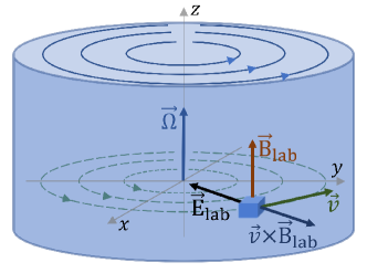
Figure 1: A charged element in a rotating plasma and the local electromagnetic fields. Note that the electric and Lorentz forces on a local element of plasma are equal in magnitude and opposite in direction.

For the configuration in Eq. (33), the Bianchi identity is satisfied identically, while the Maxwell equations take the following explicit form:

$$-\delta^{\mu}_{0}\Omega\left[2\gamma B+r\partial_{r}(\gamma B)\right]+\left(\delta^{\mu}_{1}\frac{y}{r}-\delta^{\mu}_{2}\frac{x}{r}\right)\partial_{r}(\gamma B)=en_{\textrm{eq}}\bar{u}^{\mu}-en_{\textrm{bg}}u_{\textrm{bg}}^{\mu}.$$ (34)

Here we took into account that $e\nu_{\textrm{eq}}^{\mu}=0$, which is indeed the case when $\mu_{5}=0$. Let us note in passing that major modifications would be needed in the analysis if one allows for a nonzero $\mu_{5}$. Indeed, in order to enforce the hydrodynamic equilibrium and the absence of dissipative currents at $\mu_{5}\neq 0$, additional nonzero components of the electromagnetic field would be required.

We assume that the background charge is at rest in the lab frame, i.e., $u_{\textrm{bg},1}^{\mu}=(1,0,0,0)$. (It might also be interesting to consider a comoving background with $u_{\textrm{bg},2}^{\mu}=\bar{u}^{\mu}$, but we will not investigate such a possibility in this paper.) As is easy to check, the Maxwell equations require that the magnetic field and the charge density of the plasma have the following dependence on the radial coordinate:

$$B(r) = \gamma\left(B_{0}-\frac{1}{2}en_{\textrm{bg}}\Omega r^{2}\right)\simeq B_{0}-\frac{1}{2}en_{\textrm{bg}}\Omega r^{2}+O\left(B_{0}r^{2}\Omega^{2}\right),$$ (35)

$$en_{\textrm{eq}}(r) = \gamma^{3}\left(en_{\textrm{bg}}-2B_{0}\Omega\right)\simeq en_{\textrm{bg}}-2B_{0}\Omega+O\left(en_{\textrm{bg}}r^{2}\Omega^{2}\right),$$ (36)

where $B_{0}$ is the value of the magnetic field on the rotation axis (i.e., at $r=0$). An interesting feature of this solution is that $\frac{1}{3}\nabla^{\mu}n_{\textrm{eq}}(r)-\dot{\bar{u}}^{\mu}n_{\textrm{eq}}(r)=0$ to all orders in $\Omega$. This means, in particular, that the dissipative part of the fermion number (electric) current in Eq. (20) vanishes exactly. This is quite amazing considering that the solution was obtained by solving the Maxwell equations (34) without any explicit considerations of dissipative effects.

We should remark that, in the absence of a background charge (i.e., $n_{\textrm{bg}}=0$), the solutions in Eqs. (35) and (36) appear to agree with the vortexlike solutions found in Ref. Florkowski:2018ubm . The dependence of the plasma density on the $\gamma$ factor in Eq. (36) is also consistent with the findings in Ref. Becattini:2009wh , stating that the local chemical potentials and temperature should be linear in $\gamma$: $\bar{\mu}(r)=\gamma\mu_{0}$, $\bar{\mu}_{5}(r)=\gamma\mu_{5,0}$, and $\bar{T}(r)=\gamma T_{0}$, where $\mu_{0}$, $\mu_{5,0}$, and $T_{0}$ are the values of the corresponding parameters on the rotation axis. Indeed, in the case of a charged plasma made of massless particles, such a linear dependence automatically leads to the scaling law in Eq. (36). (It is not clear, though, whether similar arguments can be generalized for a plasma made of massive particles.)

As we see from the solutions in Eqs. (35) and (36), the Maxwell equations require that the local charge density is nonzero in a rotating plasma (e.g., to the leading order in vorticity, $en_{\textrm{eq}}-en_{\textrm{bg}}\simeq-2B_{0}\Omega$). From a physics viewpoint, one might interpret this as a charge separation induced by the uniform rotation. A nonzero electric charge in the bulk is achieved by pushing the compensating charge of the opposite sign out to the cylindrical boundary of the system. Interestingly, the sign of the induced charge in the bulk is determined by the relative orientation of the magnetic field and vorticity and, thus, it can easily be flipped, for example, by changing the direction of the magnetic field.

It should be noted that a charge separation in the rotating plasma is consistent with the fact that there is a nonzero electric field in the radial direction, $\mathbf{E}_{\rm lab}=-\gamma B\Omega\mathbf{r}_{\perp}$. As mentioned earlier, the electric force of such a field on a moving element of the charged plasma is exactly compensated by the Lorentz force from the magnetic field, $\mathbf{B}_{\rm lab}=\gamma B\hat{\mathbf{z}}$; see Fig. 1. Additionally, in agreement with Ampere’s law, the circular currents of the plasma result in a total magnetic field that depends on the radial coordinate, see Eq. (35). In the presence of a background charge, moreover, the nontrivial dependence of the field on the radial coordinate appears already at the linear order in $\Omega$, i.e., $B(r)\simeq B_{0}-\frac{1}{2}en_{\textrm{bg}}\Omega r^{2}$.

IV Linearized equations of chiral hydrodynamics

In order to set the stage for a systematic study of hydrodynamic collective modes in a rotating chiral plasma, here we will discuss how to derive the linearized equations for small perturbations of the hydrodynamic quantities around their equilibrium values. In the derivation, it is beneficial to take into account the symmetry of the unperturbed state with respect to time translations, translations in the spatial $z$ direction, as well as the rotational symmetry about the $z$ axis. (Recall that both the background magnetic field and the vorticity are parallel to the $z$ axis.)

By taking into account the cylindrical symmetry in the problem, it is convenient to write down the general wavelike perturbations of (pseudo)scalar and (pseudo)vector quantities in the following form:

$$\delta s(x) = e^{-ik_{0}t+ik_{z}z+im\theta}\delta s(r),$$ (37)

$$\delta v^{3}(x) = e^{-ik_{0}t+ik_{z}z+im\theta}\delta v^{3}(r),$$ (38)

$$\delta v_{\pm}(x) = e^{-ik_{0}t+ik_{z}z+i(m\pm 1)\theta}\delta v_{\pm}(r),$$ (39)

where $s$ is a placeholder for all scalar and pseudoscalar parameters (i.e., $\mu$, $\mu_{5}$, or $T$). Similarly, the generic notations $v^{3}$ and $v_{\pm}$ stand for the longitudinal (i.e., $u^{3}$, $B^{3}$, or $E^{3}$) and transverse (i.e., $u_{\pm}$, $B_{\pm}$, or $E_{\pm}$) components of the vector quantities. Note that the plus and minus components are defined as follows: $v_{\pm}=\frac{1}{2}\left(v^{1}\pm iv^{2}\right)$. Such a separation of the longitudinal and transverse components, as well as their dependence on the cylindrical radius $r=\sqrt{x^{2}+y^{2}}$ and the polar angle $\theta=\textrm{arctan}(y/x)$, follow from the requirement that the corresponding perturbations are the eigenstates of the angular momentum operator $\hat{J}_{z}$ with the eigenvalues $m\in\mathbb{Z}$. [Note that $\hat{J}_{z}=-i\partial_{\theta}$ for scalar and pseudoscalar fields and $\hat{J}_{z}=-i\partial_{\theta}+S_{z}$ with $(S_{z})^{i}_{~{}j}=-i\varepsilon^{ij3}$ for the vector fields.] In agreement with the remaining translational symmetry, the only well-defined components of the wave vector are the timelike and longitudinal ones, i.e., $k_{0}$ and $k_{z}$, respectively.

By taking into account the constraints for the flow velocity and the electromagnetic field (i.e., $u^{\mu}u_{\mu}=1$ and $B^{\mu}u_{\mu}=E^{\mu}u_{\mu}=0$, respectively) it is clear that only three out of the total four components in each four-vector are independent. Without loss of generality, we assume that the spatial components are the independent ones. Then, as is easy to check, the deviations of the zeroth components from their equilibrium values are not independent. They are given by

$$\delta u^{0} = \Omega\left[x\delta u^{2}(x)-y\delta u^{1}(x)\right]=i\Omega r\left[e^{i\theta}\delta u_{-}(x)-e^{-i\theta}\delta u_{+}(x)\right],$$ (40)

$$\delta E^{0} = \Omega\left[x\delta E^{2}(x)-y\delta E^{1}(x)\right]=i\Omega r\left[e^{i\theta}\delta E_{-}(x)-e^{-i\theta}\delta E_{+}(x)\right],$$ (41)

$$\delta B^{0} = \Omega\left[x\delta B^{2}(x)-y\delta B^{1}(x)\right]+B\delta u^{3}(x)=i\Omega r\left[e^{i\theta}\delta B_{-}(x)-e^{-i\theta}\delta B_{+}(x)\right]+B\delta u^{3}(x).$$ (42)

It should be noted, that the general form of the perturbation to the electromagnetic field strength tensor in the lab frame can be conveniently written in terms of the perturbations of the electric and magnetic fields as follows:

$$\delta F^{\mu\nu} = \epsilon^{\mu\nu\alpha\beta}\left(\delta u_{\alpha}\bar{B}_{\beta}+\bar{u}_{\alpha}\delta B_{\beta}\right)+\delta E^{\mu}\bar{u}^{\nu}-\bar{u}^{\mu}\delta E^{\nu},$$ (43)

$$\delta\tilde{F}^{\mu\nu} = \epsilon^{\mu\nu\alpha\beta}\delta E_{\alpha}\bar{u}_{\beta}+\delta B^{\mu}\bar{u}^{\nu}-\bar{u}^{\mu}\delta B^{\nu}+\bar{B}^{\mu}\delta u^{\nu}-\delta u^{\mu}\bar{B}^{\nu},$$ (44)

where we took into account that the electric field is absent in the unperturbed state. By making use of these relations and assuming that all perturbations are small, it is straightforward to obtain a linearized system of hydrodynamic equations from Eqs. (25)–(29). The corresponding linearized equations are presented in Appendix C. Note that no explicit dependence on $t$, $z$, and $\theta$ coordinates is present in those equations because the common exponent $e^{-ik_{0}t+ik_{z}z+im\theta}$, containing such a dependence, was factored out.

In order to solve the hydrodynamic equations for collective modes, we should also specify the boundary conditions for the fields. For simplicity, we will assume that the perturbations of the scalar, pseudoscalar and longitudinal vector perturbations vanish at the boundary, i.e., $\delta s(R)=0$ and $\delta v^{3}(R)=0$, where $R$ is the cylindrical radius of the system. [Note, however, that $\delta v_{\pm}(R)=0$ cannot be enforced at the same time.] It should be clear, however, that the dispersion relations for most of the bulk modes will not be very sensitive to the choice of the boundary conditions, unless their transverse wave vectors are very small, $k_{\perp}\simeq 1/R$ (the exact definition of $k_{\perp}$ will be specified later).

IV.1 The linearized equations at vanishing vorticity

Before discussing any solutions in the most general case with a nonzero vorticity and magnetic field, let us first consider a simple setup without rotation, $\Omega=0$, but with the effects of dynamical electromagnetism fully accounted for. As will be clear, in our analysis, we also include all effects associated with the dynamical vorticity induced by collective modes themselves.

The linearized system of the hydrodynamic equations takes the following explicit form:

$$u^{\mu}\partial_{\mu}\delta n+n\partial_{\mu}\delta u^{\mu}+B^{\mu}\partial_{\mu}\delta\sigma_{B}+\frac{\tau}{3}\nabla_{\mu}\nabla^{\mu}\delta n-\tau nu^{\nu}\partial_{\mu}\partial_{\nu}\delta u^{\mu}+\frac{1}{e}\sigma_{E}\partial_{\mu}\delta E^{\mu} = 0,$$ (45)

$$u^{\mu}\partial_{\mu}\delta n_{5}+\sigma_{B}^{5}\partial_{\mu}\delta B^{\mu}+B^{\mu}\partial_{\mu}\delta\sigma_{B}^{5}+\frac{\tau}{3}\nabla_{\mu}\nabla^{\mu}\delta n_{5}+\frac{e^{2}}{2\pi^{2}\hbar^{2}}(B\cdot\delta E) = 0,$$ (46)

$$u^{\mu}\partial_{\mu}\delta\epsilon+(\epsilon+P)\partial_{\mu}\delta u^{\mu}+B^{\mu}\partial_{\mu}\delta\xi_{B} = 0,$$ (47)

$$(\epsilon+P)u^{\nu}\partial_{\nu}\delta u^{\mu}-\nabla^{\mu}\delta P+B^{\mu}u^{\nu}\partial_{\nu}\delta\xi_{B}+\frac{8\tau\epsilon}{15}\Delta^{\mu\nu}_{\alpha\beta}(\partial_{\nu}\partial^{\alpha}\delta u^{\beta})-en\delta E^{\mu}$$

$$-\epsilon^{\mu\nu\alpha\beta}\left(\frac{\tau}{3}\nabla_{\nu}\delta n-\tau nu^{\phi}\partial_{\phi}\delta u_{\nu}+\frac{1}{e}\sigma_{E}\delta E_{\nu}\right)u_{\alpha}eB_{\beta} = 0,$$ (48)

which should also be supplemented by the Maxwell equations

$$\epsilon^{\mu\nu\alpha\beta}u_{\nu}\partial_{\alpha}\delta E_{\beta}+u^{\nu}\partial_{\nu}\delta B^{\mu}+B^{\mu}\partial_{\nu}\delta u^{\nu}-B^{\nu}\partial_{\nu}\delta u^{\mu}-u^{\mu}\partial_{\nu}\delta B^{\nu} = 0,$$ (49)

$$\epsilon^{\mu\nu\alpha\beta}(u_{\nu}\partial_{\alpha}\delta B_{\beta}-B_{\nu}\partial_{\alpha}\delta u_{\beta})+u^{\mu}\partial_{\nu}\delta E^{\nu}-u^{\nu}\partial_{\nu}\delta E^{\mu}-en\delta u^{\mu}-eu^{\mu}\delta n$$

$$\qquad-e\delta\sigma_{B}B^{\mu}-\frac{e\tau}{3}\nabla^{\mu}\delta n+e\tau nu^{\phi}\partial_{\phi}\delta u^{\mu}-\sigma_{E}\delta E^{\mu} = 0.$$ (50)

The variations of the fermion number density, as well as other functions (e.g., $\delta\epsilon$ and $\delta\sigma_{B}$) are assumed to be of the most general form, i.e., $\delta n=\frac{\partial n}{\partial\mu}\delta\mu(x)+\frac{\partial n}{\partial\mu_{5}}\delta\mu_{5}(x)+\frac{\partial n}{\partial T}\delta T(x)$. They are space and time dependent, although such a dependence may not always be shown explicitly, e.g., $\delta n\equiv\delta n(x)$ and $\delta n_{5}\equiv\delta n_{5}(x)$.

In the case of vanishing vorticity, the independent wavelike solutions of the hydrodynamic equations can be conveniently expressed in terms of the cylindrical harmonics. The corresponding solutions for the local perturbations are given by Eqs. (37)–(39), with radial parts of the functions given by

$$\delta s(r) = \delta s\,J_{m}(k_{\perp}r),\quad\mbox{for}\quad s=\mu,\mu_{5},T,$$ (51)

$$\delta v^{3}(r) = \delta v^{3}\,J_{m}(k_{\perp}r),\quad\mbox{for}\quad v^{3}=u^{3},B^{3},E^{3},$$ (52)

$$\delta v_{\pm}(r) = \delta v_{\pm}\,J_{m\pm 1}(k_{\perp}r),\quad\mbox{for}\quad v_{\pm}=u_{\pm},B_{\pm},E_{\pm}.$$ (53)

Here $J_{m}(k_{\perp}r)$ is the Bessel function of the first kind and parameter $k_{\perp}$ is an analogue of the transverse wave vector for a system with cylindrical symmetry.

The linearized system (45)–(50) has the general structure $\hat{M}\delta\vec{f}=0$, where $\hat{M}$ is a $12\times 12$ matrix differential operator and $\delta\vec{f}$ is a vector consisting of all independent plasma and EM field perturbations, i.e., $\delta\vec{f}=(\delta\mu,\delta\mu_{5},\delta T,\delta\mathbf{u},\delta\mathbf{E},\delta\mathbf{B})^{T}$. By making use of the ansatz in Eqs. (37)–(39) with the radial dependence in Eqs. (51)–(53), it is easy to check that all coordinate dependence factorizes and the problem reduces to a set of homogeneous linear equations, $M\delta\vec{f}=0$, where $M$ is a $12\times 12$ algebraic matrix. For the system to have a nontrivial solution, the characteristic equation should be satisfied, i.e., $\mbox{det}(M)=0$. In essence, the latter is a polynomial equation for the frequencies of collective modes. The roots for $k_{0}$ define dispersion relations of hydrodynamic modes. In general, the corresponding frequencies (energies) are functions of the wave vectors $k_{\parallel}$ and $k_{\perp}$, as well as the eigenvalue $m$ of the angular momentum operator. The associated nontrivial solutions for $\delta\vec{f}$ (“eigenvectors”) specify the nature of the collective modes.

It is instructive to note that the above general procedure for obtaining the dispersion relations of hydrodynamic modes could easily be adjusted to take into account any boundary conditions consistent with the cylindrical symmetry. As we mentioned earlier, we will assume that the perturbations vanish at the cylindrical boundary of the system. Such boundary conditions are satisfied automatically when the values of the transverse wave vector are restricted to take only the following discrete values: $k_{\perp}^{(i)}=\alpha_{m,i}/R$, where $\alpha_{m,i}$ (with $i=1,2,...$) is the $i$th zero of the Bessel function $J_{m}(z)$. By making use of the asymptotic form for the Bessel function, we can derive the following approximate expression for the large transverse wave vectors: $k_{\perp}^{(i)}\simeq(i+m/2-1/4)\pi/R$ for $i\gg m$. By imposing the periodic boundary conditions in the $z$ direction (with period $L$), the longitudinal wave vector is discretized, i.e., $k_{z}^{(j)}=2\pi j/L$, where $j$ is an integer. When the system is large, the discretized wave vectors of both types are closely located and, thus, become almost indistinguishable from a continuum. In such a case, the discretization plays little role and could be ignored.

IV.2 The linearized equations at nonzero vorticity

In the general case of a rotating plasma, the self-consistent analysis of hydrodynamic modes becomes much more complicated. One of the primary reasons for this complication is the nontrivial radial dependence of the magnetic field and density in the unperturbed state of a uniformly rotating plasma; see Eqs. (35) and (36). In this case, the radial parts of local perturbations in Eqs. (51)–(53) can be written in the form of Fourier-Bessel series:

$$\delta s(r) = \sum_{i=1}^{\infty}\delta s^{(i)}\,J_{m}(k_{\perp}^{(i)}r),\quad\mbox{for}\quad s=\mu,\mu_{5},T,$$ (54)

$$\delta v^{3}(r) = \sum_{i=1}^{\infty}\delta v^{3}\,J_{m}(k_{\perp}^{(i)}r),\quad\mbox{for}\quad v^{3}=u^{3},B^{3},E^{3},$$ (55)

$$\delta v_{\pm}(r) = \sum_{i=1}^{\infty}\delta v_{\pm}^{(i)}\,J_{m\pm 1}(k_{\perp}^{(i)}r),\quad\mbox{for}\quad v_{\pm}=u_{\pm},B_{\pm},E_{\pm},$$ (56)

where $k_{\perp}^{(i)}=\alpha_{m,i}/R$ is the $i$th discretized value of the transverse wave vector, introduced in the previous subsection. The set of Bessel eigenfunctions used in the series above is complete and orthogonal completness1 ; completness2 . The orthogonality condition and other useful properties of the Bessel eigenfunctions are discussed in Appendix B.

By substituting perturbations (54)–(56) into the complete set of hydrodynamic equations (see Appendix C) and projecting the results onto the Bessel functions with different $k_{\perp}^{(i)}$, we arrive at an algebraic system of equations with the following block-matrix form:

$$\left(\begin{array}[]{ccc}\begin{array}[]{c}M^{(11)}\end{array}&\begin{array}[]{c}M^{(21)}\end{array}&\dots\\ \begin{array}[]{c}M^{(12)}\end{array}&\begin{array}[]{c}M^{(22)}\end{array}&\dots\\ \vdots&\vdots&\ddots\end{array}\right)\cdot\left(\begin{array}[]{c}\begin{array}[]{c}\delta\vec{f}^{(1)}\\ \delta\vec{f}^{(2)}\end{array}\\ \vdots\end{array}\right)=\left(\begin{array}[]{c}\vec{0}\\ \vec{0}\\ \vdots\end{array}\right),$$ (57)

where $M^{(ij)}$ are $12\times 12$ matrices made of the $i$th set of coefficient functions projected onto the $j$th Bessel eigenfunctions, and $\delta\vec{f}^{(i)}=(\delta\mu^{(i)},\delta\mu_{5}^{(i)},\delta T^{(i)},\delta\mathbf{u}^{(i)},\delta\mathbf{E}^{(i)},\delta\mathbf{B}^{(i)})^{T}$. Formally, Eq. (57) is an infinite system of equations. By noting, however, that the hydrodynamic description is limited to a finite range of low energies and momenta, the system can be truncated in a self-consistent way. In general, it is sufficient to limit the sum in Eqs. (54)–(56) to values of the transverse wave vector $k_{\perp}^{(i)}$ that are less than $1/l_{\rm mfp}$, where $l_{\rm mfp}$ is the mean free path of particles. In practice, though, when focusing on the low-energy part of the spectrum and/or studying the limit of small vorticity, the truncation could be even more restrictive.

Before proceeding further with the analysis, it is instructive to discuss the dependence of the matrix blocks in Eq. (57) on the angular velocity $\Omega$. As is clear from the discussion in the previous subsection, in the absence of vorticity (i.e., at $\Omega=0$), all off-diagonal blocks in Eq. (57) vanish. Indeed, in such a limit, hydrodynamic modes are characterized by well-defined values of $k_{\perp}^{(i)}$. Also, the energies of the corresponding modes are determined by the roots of the characteristic equations $\mbox{det}(M^{(ii)})=0$, where $M^{(ii)}$ are the diagonal blocks associated with specific values $k_{\perp}^{(i)}$.

At nonzero vorticity, the off-diagonal blocks in Eq. (57) do not vanish any more and, as a result, all hydrodynamic modes become nontrivial mixtures of partial waves with different values of $k_{\perp}^{(i)}$. In principle, the corresponding spectrum could be obtained by solving Eq. (57) using numerical methods. While such an approach is straightforward conceptually, it is rather tedious and is beyond the scope of this study. Instead, in the rest of this paper, we will investigate the limit of small, but nonzero vorticity.

In order to determine the spectrum of collective modes at small $\Omega$, we will solve the characteristic equations $\mbox{det}(M)=0$ to leading order in $\Omega$. While this may seem to be a very strong limitation, it should be noted that even rather optimistic estimates of vorticity in heavy-ion collisions are not that large in relative terms Becattini:2015ska ; Jiang:2016woz ; Deng:2016gyh . As is easy to check, in the limit of small $\Omega$, nontrivial corrections to the off-diagonal blocks in Eq. (57) start from the linear order terms in $\Omega$. In the calculation of $\mbox{det}(M)$, therefore, such off-diagonal matrices contribute only starting at the quadratic order in $\Omega$. This means, in particular, that all linear corrections to the dispersion relations of hydrodynamic modes are determined completely by the linear corrections to the diagonal blocks. The corresponding characteristic equations are given by $\mbox{det}(M^{(ii)}+\Omega M_{1}^{(ii)})=0$, where $M_{1}^{(ii)}\equiv(\partial M^{(ii)}/\partial\Omega)|_{\Omega=0}$.

From the above general structure of the approximate characteristic equations, it should also be clear that, to linear order in $\Omega$, the hydrodynamic modes can be unambiguously labeled by well-defined values of the transverse wave vector $k_{\perp}^{(i)}$. In other words, while the dispersion relations of the modes are modified by the vorticity, their classification remains the same as in the $\Omega=0$ case. Of course, this is hardly surprising and should have been expected since, in essence, we used a perturbation theory with $\Omega$ playing the role of a small parameter. In this connection, we should add though that, starting already from the quadratic order in $\Omega$, the off-diagonal blocks in Eq. (57) are non-negligible and a substantial mixing of partial waves with different $k_{\perp}^{(i)}$ will be unavoidable.

V Hydrodynamic modes in high temperature plasma

In this section, we study the spectrum of hydrodynamic modes in a chiral rotating plasma at high temperature, i.e., $T\gg\mu$, or, in other words, we assume that the fermion number chemical potential is small compared to the temperature. As is clear, such a regime is most suitable for describing hot plasmas in the early universe and in heavy-ion collisions. The opposite limit, i.e., $T\ll\mu$, will be addressed in the next section.

Before proceeding to the technical part of the study, it is instructive to discuss the general validity of the hydrodynamic approach and the hierarchy of various length scales in the problem at hand. The shortest length scale of relevance is the de Broglie wavelength for chiral particles $l_{d}\simeq\hbar/T$ (at high density, it will be replaced by $l_{d}\simeq\hbar/\mu$). Clearly, the hydrodynamic description cannot work on such short microscopic distances. In fact, it becomes relevant only on the scales much larger than the particle mean free path, i.e., $l_{\rm mfp}\simeq\tau$ (recall that $c=1$ in the units used here), where the definition of local equilibrium could be meaningful. In a background magnetic field, there is an additional scale defined by the magnetic length $l_{B}=\sqrt{\hbar/eB}$. We will assume that the field is weak in the sense that $\sqrt{\hbar eB}\ll T$, which is usually the case in most applications. This implies that $l_{d}\ll l_{B}$. The magnetic length could, however, be comparable to the mean free path. In fact, the hierarchy between the two scales could be used to distinguish the regime of very weak fields, i.e., $l_{B}\gtrsim l_{\rm mfp}$, from that of moderately strong fields, i.e., $l_{B}\lesssim l_{\rm mfp}$.

When discussing hydrodynamic modes, we will have to deal with yet another window of length scales, defined by the wavelengths of the modes, i.e., $\lambda_{k}\simeq 1/k$, where $k$ is the corresponding wave vector. Clearly, the hydrodynamic description for such modes makes sense only if $\lambda_{k}\gg l_{\rm mfp}$ (or, equivalently, $k\ll 1/l_{\rm mfp}$). In a finite system, at the same time, the maximum wavelength is limited by the size of the system itself, $\lambda_{k}\lesssim R$. Finally, the size of a uniformly rotating relativistic plasma is limited by the scale of $\Omega^{-1}$. Therefore, in the analysis of collective modes below, we will assume the following hierarchy of scales: $l_{d}\ll l_{B}\lesssim l_{\rm mfp}\ll\lambda_{k}\lesssim R\ll\Omega^{-1}$. This hierarchy will also be used in the derivation of analytical results. In order to simplify the task of keeping track of different scales, it will be convenient to use the following values and ranges of dimensionless parameters:

$$l_{\rm mfp}\Omega\simeq\xi^{2},\qquad\xi^{3/2}\simeq\frac{l_{\rm mfp}}{R}\lesssim kl_{\rm mfp}\lesssim\xi^{1/2},\qquad\frac{l_{\rm mfp}}{l_{B}}\simeq\xi^{-1/4},\qquad\frac{l_{\rm mfp}}{l_{d}}\simeq\xi^{-1},$$ (58)

where we introduced a small parameter $\xi\simeq 10^{-2}$ in order to easily separate all relevant scales in the problem. While concentrating on the high-temperature regime here, it might be interesting to see how the effects of a small chemical potential start showing up in the spectrum of collective modes. Therefore, we also include a nonzero $\mu$, but assume that its value is very small, e.g., $|\mu|\simeq\xi^{2}T$ (or, equivalently, $|\mu|l_{d}\simeq\xi^{2}\hbar$).

V.1 Charged plasma at $\Omega=0$

Before addressing hydrodynamic modes at nonzero vorticity, it is instructive to set up the stage by first discussing the benchmark results at $\Omega=0$. As expected in the hydrodynamic regime, there are generically two very different types of modes: propagating and diffusive. The dispersion relations of the former ones have nonzero real parts and relatively small imaginary parts. The diffusive modes, on the other hand, have either no real parts at all, or the imaginary parts much larger than real ones.

By solving the linearized equations (45)–(50), we find that there are two kinds of propagating modes at $\Omega=0$, namely, a sound wave with the dispersion relation given by

$$k_{0}=\frac{s_{e}k}{\sqrt{3}}-\frac{2}{15}i\tau k^{2},$$ (59)

and an Alfvén wave with the dispersion relation approximately given by

$$k_{0}^{(\pm)}=s_{e}\frac{3\sqrt{5}B\hbar^{3/2}k_{z}}{\sqrt{7}\pi T^{2}}\left(1\pm\frac{\sqrt{5}e\mu}{2\sqrt{7}\pi\hbar^{3/2}k}\right)-\frac{1}{10}i\tau k^{2}.$$ (60)

In both cases, $k=\sqrt{k_{z}^{2}+k_{\perp}^{2}}$ and $s_{e}=\pm 1$. As is clear, both choices of $s_{e}$ (i.e., the overall sign in front of the real part of the energy) correspond to the same mode. In most cases, the signs $s_{e}$ could be associated simply with different directions of propagation. As is easy to check, in fact, this is the case for the Alfvén waves in Eq. (60).

The sound wave in Eq. (59) describes the propagation of longitudinal elastic deformations in plasma. The propagation of such a wave does not induce any local oscillations of the electric charge and, as a result, there are no dynamical electromagnetic fields induced. Also, as expected for the ultrarelativistic matter, the speed of sound $c_{s}$ is determined by its compressibility, $c_{s}^{2}=\partial P/\partial\rho=1/3$. (As we mentioned earlier, in a more realistic case of a strongly interacting quark-gluon plasma, the value of $c_{s}^{2}$ is expected to be somewhat smaller than $1/3$ Bazavov:2014pvz , but there is no reason to expect that the nature of the corresponding sound mode will change qualitatively.)

A few words are in order about the Alfvén waves with the dispersion relations given by Eq. (60). These are magnetohydrodynamic modes with two possible circular polarizations: the left-handed one with $\delta u_{+}\ll\delta u_{-}$ and the right-handed one with $\delta u_{+}\gg\delta u_{-}$. From the viewpoint of the fluid flow oscillations, these are transverse modes. The energies of the corresponding two branches of waves differ slightly because the term with the chemical potential $\mu$ comes with opposite signs. In the limit $\mu\to 0$, the speed of propagation of these waves is the same for both polarizations. As is easy to check by neglecting the dissipative effects, the expression for the speed can also be written as $v_{A}=B/\sqrt{\epsilon_{\textrm{eq}}+P_{\textrm{eq}}}$, which is the standard expression for the Alfvén waves in a relativistic plasma Harris . It might be appropriate to mention that the propagation of Alfvén waves is accompanied by the fluid flow oscillations with nonzero local dynamical vorticity.

Here it might be appropriate to note that the analytical expressions in Eq. (60) were obtained by using the expansion in small parameter $\xi$, which was introduced in Eq. (58) in order to separate different scales in the problem. Therefore, while the corresponding dispersion relations provide good analytical approximations, they cannot be extended to the regions of very small and very large values of the wave vector. In order to support the validity of the approximate results obtained analytically, we compare them in Fig. 2 with the dispersion relations found numerically. The panels in Fig. 2 show the results for the real (red lines and points) and imaginary (blue lines and points) parts of the energy at three different fixed values of the magnetic field, i.e., $\hbar eB/T^{2}=0.5\times 10^{-3}$, $\hbar eB/T^{2}=1\times 10^{-3}$, and $\hbar eB/T^{2}=1.5\times 10^{-3}$, respectively. Note that, for the model parameters used, the hydrodynamic regime breaks down in the gray shaded regions at small and large values of $k_{z}$. As is clear from Fig. 2, the analytical relations approximate well the numerical results basically in the whole region where the real part of the energy remains larger than its imaginary part, i.e., $\mbox{Re}(k_{0})\gtrsim\mbox{Im}(k_{0})$.

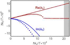
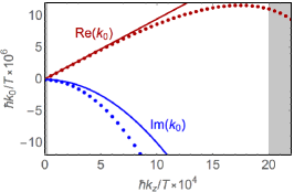
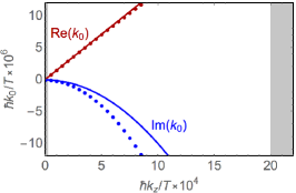
Figure 2: The comparison of the approximate analytical results (solid lines) for the real (red lines and points) and imaginary (blue lines and points) parts of the energy for the Alfvén waves with the corresponding numerical results (points) at $\Omega=0$ for three fixed values of the magnetic field: $\hbar eB/T^{2}=0.5\times 10^{-3}$ (left panel), $\hbar eB/T^{2}=10^{-3}$ (middle panel), and $\hbar eB/T^{2}=1.5\times 10^{-3}$ (right panel). The real and imaginary parts of the energy are shown in red and blue, respectively. The other model parameters are $\tau T/\hbar=10^{2}$, $\mu/T=10^{-4}$, and $\hbar k_{\perp}/T=10^{-4}$.

In addition to the propagating modes, there are also two types of purely diffusive modes. The latter include the electric field decay mode with

$$k_{0}=-\frac{e^{2}}{9\hbar^{3}}i\tau T^{2}$$ (61)

and the chiral charge diffusive mode described by

$$k_{0}=-\frac{1}{3}i\tau k^{2}-i\frac{27e^{2}B^{2}\hbar^{2}}{4\pi^{4}\tau T^{4}}.$$ (62)

It should be noted that there are three degenerate modes with the dispersion relation in Eq. (61), which correspond to three different polarizations of the electric field. The origin of these modes can be traced back to Ampere’s law that takes a particularly simple approximate form $\partial_{t}\mathbf{E}+\sigma_{E}\mathbf{E}\approx 0$. This is also reconfirmed by the fact that the imaginary part in Eq. (61) is completely determined by the electrical conductivity, $\mbox{Im}(k_{0})=-\sigma_{E}$.

Before concluding this section, we would like to emphasize that there is no propagating mode in the spectrum that could be identified with the chiral magnetic wave. It is natural to ask, therefore, what is the reason for its absence. As we explain in Appendix D in detail, the chiral magnetic wave is overdamped because of a high conductivity of hot plasma, which causes a rapid screening of the electric charge fluctuations and, thus, prevents the wave from forming. While the situation is slightly more complicated in the strongly coupled quark-gluon plasma created in heavy-ion collisions, the chiral magnetic wave is still strongly overdamped due to the combined effects of electrical conductivity and charge diffusion Shovkovy:2018tks .

V.2 Charged plasma at $\Omega\neq 0$

Let us now discuss the spectrum of hydrodynamic modes in the case of small, but nonzero vorticity. As mentioned earlier, in order to simplify the analysis, we will limit ourselves only to linear order corrections to the dispersion relations in powers of $\Omega$. In such an approximation, the modes are classified by the same values of $k_{\perp}^{(i)}$ as at $\Omega=0$. Since there is no mixing of partial waves with different values of $k_{\perp}^{(i)}$, we will utilize a simpler notation $k_{\perp}$ instead of $k_{\perp}^{(i)}$ in the rest of the paper.

Let us start by noting that the dispersion relation of the sound wave receives a linear correction in vorticity, i.e.,

$$k_{0}=\frac{s_{e}k}{\sqrt{3}}-\frac{2}{15}i\tau k^{2}+m\Omega\left(\frac{2}{3}+\frac{5e^{2}\mu^{2}}{14\pi^{2}\hbar^{3}k^{2}}\right).$$ (63)

As in the case of vanishing vorticity, it remains a longitudinal wave. Its propagation is sustained primarily by oscillations of temperature $\delta T$ and velocity $\delta u^{\mu}$. However, at nonzero $\mu$, the wave could also excite small perturbations of the electromagnetic fields.

To the leading linear order in the angular velocity $\Omega$, the dispersion relations of the Alfvén waves are given by the following approximate expression:

$$k_{0}^{(\pm)}=m\Omega+s_{e}k_{z}\sqrt{\frac{45\mathcal{B}_{\pm}^{2}\hbar^{3}}{7\pi^{2}T^{4}}+\left(\frac{\Omega}{k}-\frac{15e\mathcal{B}_{\pm}\mu}{14\pi^{2}T^{2}k}\right)^{2}}\pm k_{z}\left(\frac{\Omega}{k}-\frac{15e\mathcal{B}_{\pm}\mu}{14\pi^{2}T^{2}k}\right)-i\tau k^{2}\left(\frac{1}{10}+\frac{9\hbar^{3}}{2e^{2}\tau^{2}T^{2}}\right),$$ (64)

where we introduced the following shorthand notation:

$$\mathcal{B}_{\pm}=B-\frac{en_{\rm eq}\Omega}{6k_{\perp}^{2}}\left[2(m\pm 1)(m\pm 2)+k_{\perp}^{2}R^{2}\right].$$ (65)

Note that we used $n_{\rm bg}=n_{\rm eq}$, which enforces the electric charge neutrality in the plasma at $\Omega=0$, see Eq. (36). As we can see, there are four different branches of Alfvén waves. They are determined by two different circular polarizations, labeled by the $\pm$ signs in Eq. (64), and two directions of propagation with respect to the $z$ axis. The latter are formally distinguished by $s_{e}=\pm 1$. (Recall that both the background magnetic field and the axis of rotation are parallel to the $z$ axis.)

By comparing the result in Eq. (64) with the dispersion relation at $\Omega=0$, given by Eq. (60), we see that the inclusion of vorticity lifts the degeneracy of modes propagating in opposite directions with respect to the background magnetic field (and/or vorticity). Moreover, we also find that the propagation of these types of waves is modified by the chiral vortical effect. This is most pronounced in the case of small $k_{z}$ (i.e., $k_{z}\lesssim k_{\perp}$). In such a case, therefore, it might be suitable to call these modes the Alfvén-vortical waves. The dispersion relations for several modes with different values of the angular momentum $m$ are shown in Fig. 3. (The hydrodynamic regime breaks down in the gray shaded regions at small and large values of $k_{z}$.) Note that the approximate analytical expressions (represented by solid lines) are in good agreement with the numerical results (shown with dots) in the region of small momenta.

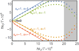
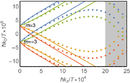
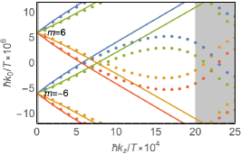
Figure 3: The real parts of the energies of the Alfvén waves with different values of the angular momentum: $m=0$ (left panel), $m=\pm 3$ (middle panel), and $m=\pm 6$ (right panel). The other model parameters are $\tau T/\hbar=10^{2}$, $\mu/T=10^{-4}$, $\hbar\Omega/T=10^{-6}$, $\hbar eB/T^{2}=10^{-3}$, $RT/\hbar=10^{4}\alpha_{0,1}\approx 2.4\times 10^{4}$, and $k_{\perp}=\alpha_{m,1}/R$.

It is interesting to note that the energies of the circularly polarized Alfvén waves depend on the magnetic field only via the combinations $\mathcal{B}_{\pm}$, defined in Eq. (65). This means that one of the circularly polarized waves with a fixed angular momentum $m$ could be fine-tuned (e.g., by adjusting the magnetic field so that $\mathcal{B}_{-}=0$) into a pure chiral vortical wave with the dispersion relation given by $k_{0}\approx m\Omega+(s_{e}-1)\frac{k_{z}}{k}\Omega-\frac{1}{10}i\tau k^{2}$.

For completeness, let us now briefly discuss the diffusive modes. The electric field decay mode remains the same as in Eq. (61). As for the chiral charge diffusive mode, at nonzero $\Omega$, it is given by

$$k_{0}=m\Omega-i\frac{27(e\mathcal{B}_{0})^{2}\hbar^{2}}{4\pi^{4}\tau T^{4}}-\frac{1}{3}i\tau k^{2},$$ (66)

where we introduced the following shorthand notation:

$$\mathcal{B}_{0}=B-\frac{en_{\rm eq}\Omega}{6k_{\perp}^{2}}\left[2(m-1)(m+1)+k_{\perp}^{2}R^{2}\right].$$ (67)

Note that the energy of the chiral charge diffusive mode has a nonzero real part proportional to $\Omega$. One might speculate, therefore, that under certain conditions and beyond the leading order in $\Omega$, it may even become a propagating mode. As is easy to check, the chiral charge diffusive mode is determined primarily by the corresponding continuity relation. At nonzero $\Omega$, in particular, the latter can be approximately given by

$$\partial_{0}n_{5}=-\frac{\tau}{3}\nabla^{2}n_{5}-(\bm{\Omega}\times\bm{\nabla}n_{5})\cdot\bm{r}_{\perp}.$$ (68)

By solving this, we can indeed reproduce the first and the last terms in the dispersion relation (66). This reconfirms that, while other degrees of freedom may influence this diffusive mode in principle, their role is minor.

V.3 Charged plasma at $\Omega\neq 0$ without dynamical electromagnetic fields

As we argued in Sec. II by using rather general arguments, a self-consistent treatment of charged chiral plasma requires a proper inclusion of fully dynamical electromagnetic fields. In this subsection, we test the validity of such a claim by performing a comparative study without the inclusion of the dynamical fields. In order to achieve such a regime in the charged chiral plasma, we will assume that the matter is affected only by the static background magnetic field. No additional background electric fields can be allowed because those would drive dissipative Ohm currents. When neglecting dynamically induced electromagnetic fields, there will be no effect from such fields on the plasma modes. As we will see, many signature features of hydrodynamic modes will be lost in such an approximation. This finding, therefore, will reconfirm the importance of accounting for the dynamical fields.

When dynamical electromagnetic fields are neglected, the Maxwell equations play no role in determining the properties of hydrodynamic modes. This means that one is left with the system of only six continuity equations (25)–(28). To leading order in $\Omega$, we can assume that the background values of the chemical potential and temperature are spatially uniform. In the absence of the background electric field, the chiral anomaly is effectively switched off. This means that both fermion number (electric) and chiral currents are conserved and affect collective modes in similar ways.

We find that there are three kinds of propagating hydrodynamic modes: a longitudinal sound wave, a transverse vortical wave, and a transverse chiral magnetic wave. (Note that the terms longitudinal and transverse refer to the direction of fluid flow oscillations with respect to the wave vector.) Their dispersion relations read

$$k_{0} = \frac{s_{e}k}{\sqrt{3}}+\frac{2}{3}m\Omega-\frac{2}{15}i\tau k^{2},$$ (69)

$$k_{0} = m\Omega+s_{e}\frac{2k_{z}\Omega}{k}-\frac{1}{5}ik^{2}\tau,$$ (70)

$$k_{0} = m\Omega+s_{e}\frac{3e\mathcal{B}_{0}\hbar k_{z}}{2\pi^{2}T^{2}}-\frac{1}{3}ik^{2}\tau,$$ (71)

respectively. As expected, the sound mode is not affected much by omitting dynamical electromagnetic fields. However, it did become completely independent of the chemical potential. This should have been expected though since oscillations of local electric fields from charge density perturbations are artificially switched off now.

The modes in Eq. (70) are substitutes for the Alfvén waves (64) in the fully dynamical case. By comparing their dispersion relations, we clearly see that the modes are drastically different. This is further confirmed by reviewing the underlying nature of the two sets of modes. For example, the vortical wave (70) is driven almost exclusively by velocity perturbations $\delta u^{\mu}$. A pair of the weakly damped chiral magnetic waves (71) is driven by oscillations of either left-handed ($s_{e}=-1$) or right-handed ($s_{e}=1$) particles. As expected, they replace a pair of diffusive modes found in the dynamical regime in the previous subsection. At $\mathcal{B}_{0}=0$, they turn again into diffusive electric and chiral charge waves, driven by the perturbations of $\delta\mu$ and $\delta\mu_{5}$, respectively.

To summarize the results of this subsection, we find that neglecting dynamical electromagnetic fields has a profound effect on the spectrum of collective modes in the hydrodynamic regime. One of them is the appearance of propagating chiral magnetic waves, which are absent in the charged chiral plasma with dynamical electromagnetism. The other qualitative difference is the absence of the correct Alfvén waves, which are replaced by the vortical wave with a rather different dispersion relation.

V.4 Plasma of neutral particles at $\Omega\neq 0$

For completeness, it might also be interesting to discuss the hydrodynamic modes in a chiral plasma made of neutral particles. Clearly, the Maxwell equations play no role in this case. The hydrodynamic description is governed by Eqs. (25)–(28) with the vanishing electromagnetic fields. To leading order in $\Omega$, the values of the chemical potential $\mu$ and temperature $T$ for the uniformly rotating neutral plasma can be assumed constant in the global equilibrium. Moreover, we can even include an arbitrary nonzero axial chemical potential $\mu_{5}$.

Among the propagating modes in neutral plasma, we find the usual longitudinal sound wave with the dispersion relation given by

$$k_{0}=\frac{s_{e}k}{\sqrt{3}}+\frac{2}{3}m\Omega-\frac{2}{15}i\tau k^{2},$$ (72)

where $s_{e}=\pm 1$, and a single circularly polarized vortical wave with the dispersion relation

$$k_{0}=m\Omega+s_{e}\frac{2k_{z}\Omega}{k}-\frac{1}{5}i\tau k^{2}.$$ (73)

It should be emphasized that the sign $s_{e}=\pm 1$ defines one of the two possible directions of propagation of the vortical wave with respect to the $z$ axis. For each direction of the propagation, though, there is only one circularly polarized mode. This differs qualitatively from the Alfvén-vortical waves in charged plasmas which have two propagating circularly polarized modes for each direction.

The dispersions of diffusive modes associated with the fermion number charge and the chiral charge are degenerate and resemble the zero-field limit of that in Eq. (66). In particular, they are given by

$$k_{0}=m\Omega-\frac{1}{3}i\tau k^{2}.$$ (74)

It is rather interesting to point out that, to leading order in $\Omega$, the equilibrium values of the chemical potentials $\mu$ and $\mu_{5}$ do not affect the energy spectrum of the modes in the neutral chiral plasma. The spectra also are not dependent on temperature.

VI Hydrodynamic modes in dense plasma

In this section, we study the spectrum of hydrodynamic modes in a chiral rotating plasma at high density, i.e., $\mu\gg T$. Such a regime could be realized in compact stars and, perhaps, also in Dirac and Weyl materials, in which low-energy electron quasiparticles behave as pseudorelativistic chiral fermions.

As in the case of hot plasma in the previous section, it is convenient to use a specific hierarchy of all relevant scales in the problem by relating them via a single small parameter $\xi\simeq 10^{-2}$. In the case of dense plasma, we will use

$$l_{\rm mfp}\Omega\simeq\xi^{5/2},\qquad\xi^{3/2}\simeq\frac{l_{\rm mfp}}{R}\lesssim kl_{\rm mfp}\lesssim\xi^{1/2},\qquad\frac{l_{\rm mfp}}{l_{B}}\simeq\xi^{-1/4},\qquad\frac{l_{\rm mfp}}{l_{d}}\simeq\xi^{-1}.$$ (75)

It should be noted that here we consider even smaller vorticity in relative terms than in hot chiral plasma, see Eq. (58). This is motivated by the need to keep the vorticity corrections to the magnetic field (67) and (65) under control in the regime of a large fermion number density. While considering the high-density regime, it is instructive to see how the effects of a small temperature start showing up in the spectrum of collective modes. For this purpose, we include a nonzero temperature, but assume that its value is small, e.g., $T\simeq\xi\mu$ (or, equivalently, $Tl_{d}\simeq\xi\hbar$, where $l_{d}=\hbar/\mu$).

VI.1 Charged plasma at $\Omega=0$

Before considering the case of nonzero vorticity, we review the spectrum of hydrodynamic modes in the case $\Omega=0$ by solving the linearized system of equations (45)–(50). As expected, we find that there are two kinds of propagating modes at $\Omega=0$, namely, plasmons and helicons. Also, there are two diffusive modes with identical dispersions, $k_{0}=-i\tau k^{2}/3$. Note that, in the regime of dense matter, there are no usual sound waves. They are replaced by plasmons. Similarly, the Alfvén waves are morphed into helicons.

Plasmons describe the propagation of charge oscillations sustained by dynamically induced electric fields. As is well known, their frequency for the ultrarelativistic plasma without background fields and rotation is given by $\omega_{\textrm{PL}}=\frac{e\mu}{\sqrt{3}\pi\hbar^{3/2}}$. The plasmon can have three degenerate modes with different polarizations. We find that the degeneracy is lifted by the magnetic field. Indeed, from our linearized system of equations, we find that the dispersion relations of the plasmon modes are given by

$$k_{0}^{(s)}=s_{e}\frac{e\mu}{\sqrt{3}\pi\hbar^{3/2}}+s\frac{eB}{2\mu}-\frac{ie^{2}\tau T^{2}}{18\hbar^{3}}-\frac{1}{10}i\tau k^{2},$$ (76)

where $s_{e}=\pm 1$ and $s=-1,0,1$. In terms of the hydrodynamic variables, plasmons are primarily driven by the oscillations of flow velocity $\delta u_{\pm}$ and electric field $\delta E_{\pm}$. For $s=\pm 1$, the modes have clockwise (with nonzero $\delta u_{+}$ and $\delta E_{+}$) and anticlockwise (with nonzero $\delta u_{-}$ and $\delta E_{-}$) circular polarizations, respectively. The case of $s=0$ corresponds to the mode with the linear polarization in the $z$ direction.

The dispersion relations of the helicon mode are given by

$$k_{0}=s_{e}\frac{3\pi^{2}eBkk_{z}\hbar^{3}}{e^{2}\mu^{3}}-\frac{3\pi^{2}\hbar^{3}}{5e^{2}\mu^{2}}i\tau k^{4},$$ (77)

where $s_{e}=\pm 1$. One of the signature features of such magnetohydrodynamic modes is their quadratic dispersion relations. They are circularly polarized with a given handedness, determined by the sign of $s_{e}$. In terms of the hydrodynamic variables, the propagation of helicons is driven primarily by oscillations of flow velocity $\delta u_{\pm}$, temperature $\delta T$, and magnetic field $\delta B_{\pm}$. It might be appropriate to mention that, for a typical choice of the model parameters with the hierarchy of scales in Eq. (75), the helicons are well-defined propagating (rather than overdamped) modes in the whole region of momenta, $\xi^{3/2}\lesssim kl_{\rm mfp}\lesssim\xi^{1/2}$. This remains also marginally true even for a range of somewhat weaker magnetic fields, provided $l_{\rm mfp}/l_{B}\gtrsim 1$. However, in the case of very weak fields, the helicons will become overdamped already at some intermediate values of the wave vector (e.g., $kl_{\rm mfp}\simeq\xi^{3/4}$ when $l_{\rm mfp}/l_{B}\simeq\xi^{1/4}$).

VI.2 Charged plasma at $\Omega\neq 0$

Let us now proceed to the case of a rotating chiral plasma. As in the case of hot plasma in the previous section, we will study the modifications of hydrodynamic modes up to linear order in $\Omega$. In this case, the modes are classified by well-defined transverse wave vectors $k_{\perp}$. (Recall that the corresponding values are discretized $k_{\perp}^{(i)}=\alpha_{m,i}/R$, but we will omit the superscript in order to simplify the presentation.)

We start by noting that the $\Omega=0$ plasmon dispersion relation given by Eq. (76) remains almost the same, but the magnetic field $B$ in the subleading term is replaced by $\mathcal{B}_{s}$, i.e.,

$$k_{0}^{(s)}=s_{e}\frac{e\mu}{\sqrt{3}\pi\hbar^{3/2}}+s\frac{e\mathcal{B}_{s}}{2\mu}-\frac{ie^{2}\tau T^{2}}{18\hbar^{3}}-\frac{1}{10}i\tau k^{2}.$$ (78)

As for the helicon mode, its dispersion relation becomes

$$k_{0}=m\Omega\left(\frac{1}{2}-\frac{k_{z}^{2}}{k_{\perp}^{2}}\right)+s_{e}\sqrt{\frac{m^{2}\Omega^{2}}{4}+\frac{9\pi^{4}(\mathcal{B}_{+}+\mathcal{B}_{-})^{2}k^{2}k_{z}^{2}\hbar^{5}}{4\mu^{6}}}-\frac{3\pi^{2}\hbar^{3}}{5e^{2}\mu^{2}}i\tau k^{4},$$ (79)

where $s_{e}=\pm 1$. As is easy to see, the positive branches of the real part of energy (i.e., $s_{e}=+1$) are gapped for $m>0$ and gapless for $m\leq 0$. Concerning the case of $m>0$, the values of the gaps are determined by the angular velocity, $m\Omega$. A typical spectrum is illustrated in Fig. 4, where the dispersion relations for several fixed values of the angular momentum ($m=-4,-2,0,2,4$) are shown. Note that, in the figure, we zoomed into the region of very small energies. By taking into account that $\Omega$ is very small, it should be clear that the complete spectrum contains a nearly continuous range of gaps.

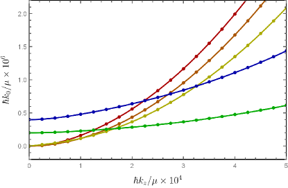
Figure 4: The positive branches of the real part of helicon energies for several values of the angular momentum, i.e., $m=-4$ (red line), $m=-2$ (orange line), $m=0$ (olive line), $m=2$ (green line), and $m=4$ (blue line). The other model parameters are $\hbar eB/\mu^{2}\approx 2\times 10^{-3}$, $\tau\mu/\hbar=100$, $\hbar\Omega/\mu=10^{-7}$, and $k_{\perp}=\alpha_{m,1}/R$.

It is interesting to note that for certain values of the angular momentum (when the magnetic field is fixed), the effective field $(\mathcal{B}_{+}+\mathcal{B}_{-})$ could become very small, or even zero. In this case, the first term in the dispersion relation (79) dominates and leads to a quadratic dependence on $k_{z}$ with a negative overall coefficient. (Note that the energies for the branches with negative values of $m$ have opposite signs.)

From a physics viewpoint, the negative curvature of the dispersion relation as a function of $k_{z}$ implies that the group velocity of such modes $v_{z}$ is negative. This is a rather interesting feature that, potentially, could be important in applications. By analyzing the analytical expression in Eq. (79), we find, however, that a negative group velocity can be realized only for rather large magnetic fields. Indeed, by making use of the properties of the Bessel functions, we find that the negative slope is possible only when the magnetic field lies in the following window: $en_{\rm eq}R^{2}\Omega/6<B<en_{\rm eq}R^{2}\Omega/2$. This corresponds to the dimensionless ratio $l_{\rm mfp}/l_{B}\simeq\xi^{-7/4}(e/\sqrt{\hbar})$, which is substantially larger than $1$ even for a rather small coupling constant, $e/\sqrt{\hbar}=1/\sqrt{137}$. The ranges of angular momenta $m$ of the modes with $v_{z}<0$ are illustrated graphically in Fig. 5. There we show three colored bands that correspond to the three smallest values of the transverse momenta $k_{\perp}^{(i)}$ with $i=1,2,3$. As we see, the ranges of bands in $m$ rise very steeply as $B/(en_{\rm eq}R^{2}\Omega)$ approaches $1/2$. The bands also have a tendency to shift upwards with increasing $k_{\perp}^{(i)}$.

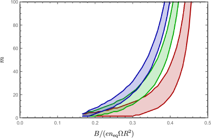
Figure 5: The ranges of angular momenta $m$ for which helicon modes can have negative group velocity. The colored bands correspond to three smallest values of the transverse momenta $k_{\perp}^{(i)}$ with $i=1,2,3$ (from red to blue, respectively).

In addition to the propagating modes, there is also a pair of overdamped modes associated with the diffusion of chiral charge and energy, i.e.,

$$k_{0} = m\Omega-\frac{1}{3}i\tau k^{2},$$ (80)

$$k_{0} = m\Omega\left(1-\frac{e^{2}\mu^{2}\tau^{2}}{9\pi^{2}\hbar^{3}}\right)-\frac{1}{3}i\tau k^{2},$$ (81)

respectively. In the hydrodynamic regime defined by the hierarchy of length scales in Eq. (75), neither of these modes has a chance of becoming a well-resolved propagating mode.

VI.3 Charged plasma at $\Omega\neq 0$ without dynamical electromagnetic fields

As in the case of hot plasma in the previous section, here it is also instructive to verify that the description of hydrodynamic modes is substantially modified in the background-field approximation, i.e., when the dynamical electromagnetic fields are neglected.

Switching off the dynamical electromagnetic fields is equivalent to ignoring the Maxwell equations. Then the simplified system of the six linearized equations contains only continuity equations (25)–(28). Here we will concentrate on the propagating modes, which are particularly interesting. As for the diffusive modes, one can verify that there are two degenerate modes with the dispersion relation given by Eq. (80).

One of the immediate consequences of the approximation without dynamical electromagnetic fields is the absence of the plasmons in the spectrum. They are replaced by the sound waves with the energy given by

$$k_{0}=\frac{s_{e}k}{\sqrt{3}}+\frac{2}{3}m\Omega-\frac{2}{15}i\tau k^{2}.$$ (82)

The underlying physics of such a dramatic change is clear. While neglecting the Gauss law, local oscillations of the electric charge density do not produce any electric field, resulting in a gapless sound wave exactly as in the case of plasma made of neutral particles.

While the helicon remains in the spectrum, its dispersion relation is substantially modified. In particular, its energy in the background-field approximation is given by

$$k_{0}=m\Omega+\frac{s_{e}}{5\mu}e\mathcal{B}_{s}kk_{z}\tau^{2}-\frac{1}{5}i\tau k^{2},$$ (83)

where $s_{e}=\pm 1$. In essence, this is a purely hydrodynamic mode, which is driven by oscillations of the fluid velocity. Its propagation is accompanied by oscillations of temperature, as well as small oscillations of the electric and chiral chemical potentials.

VI.4 Chiral plasma of neutral particles at $\Omega\neq 0$

For completeness, let us also discuss the case of chiral plasma made of neutral particles. Since the chiral anomaly is absent in this case, it is straightforward to include a nonzero chiral chemical potential $\mu_{5}$ along with the fermion number chemical potential $\mu$. Note, however, that none of the hydrodynamic modes in this regime will be modified by the values of $\mu_{5}$ and $\mu$. This situation is qualitatively the same as in the case of hot plasma made of neutral particles. Also, as in that case, the spectra do not depend on temperature.

The energies of the sound and vortical waves are given by the following expressions:

$$k_{0} = \frac{s_{e}k}{\sqrt{3}}+\frac{2}{3}m\Omega-\frac{2}{15}i\tau k^{2},$$ (84)

$$k_{0} = m\Omega+s_{e}\frac{2k_{z}\Omega}{k}-\frac{1}{5}i\tau k^{2},$$ (85)

respectively. While the former is a longitudinal wave, the latter is a transverse circularly polarized one. There is also a pair of degenerate diffusion modes with the dispersion relation given by Eq. (80).

VII Summary

In this paper, we used a covariant formulation of the chiral kinetic theory Hidaka:2016yjf ; Hidaka:2017auj in the relaxation-time approximation in order to derive the first-order dissipative hydrodynamics equations for a magnetized chiral plasma with nonzero vorticity. By noting that dynamical electromagnetism should play a profound role in such a relativistic charged plasma, we argued that the complete set of hydrodynamic equations should necessarily include the appropriate Maxwell equations.

Furthermore, by utilizing the corresponding hydrodynamic framework with dynamical electromagnetism, we derived the complete spectrum of hydrodynamic modes almost completely by analytical methods. The task of solving the linearized equations was greatly simplified by assuming that the plasma is confined to a cylindrical region of finite radius $R$ rotating uniformly with a small angular velocity $\Omega$. Then, by imposing suitable boundary conditions, at linear order in $\Omega$, we were able to classify all modes in terms of the angular momenta $m$ and the transverse wave vectors $k_{\perp}^{(i)}$. The latter, in particular, are determined by the inverse radius $R^{-1}$, multiplied by the zeros of the Bessel functions. Such a setup provides a rigorous and systematic way not only for including the combined effects of the background magnetic field and rotation but also for treating systems of finite size.

One of the critical details in our analysis of hydrodynamic modes is self-consistent determination of the unperturbed (equilibrium) state for a charged plasma rotating with a constant angular velocity. As we showed, relativistic effects force the corresponding state to be nonuniform in the radial direction. The situation is further complicated by the possible presence of a static background of nonchiral particles, in which case the nonuniformity shows up already at the linear order in $\Omega$. We verified that (i) the electric and magnetic forces on any element of the rotating plasma are exactly compensated, and (ii) there are no dissipative hydrodynamic processes in the correct equilibrium state.

The main results of this paper also include detailed spectra of hydrodynamic modes in the regimes of both high temperature and high density. In the case of hot plasmas, the main propagating modes are the sound and Alfvén waves. At high density, on the other hand, the corresponding modes are the plasmons and the helicons. In all regimes, the dispersion relations are affected in a rather nontrivial way by a nonzero angular velocity $\Omega$. One of the notable exceptions is the plasmon, which remains intact up to the linear order in $\Omega$. It is almost certain, of course, that its energy will be changed at higher orders in $\Omega$, but our approximation was insufficient to reconfirm this explicitly. We also tested directly that dynamical electromagnetism plays an important role in determining qualitative properties of all well-resolved (i.e., not overdamped) propagating modes. This was done by comparing the results with and without the inclusion of the dynamical fields. We found that the spectra of collective modes also include a number of diffusive (overdamped) modes.

At the end, we would like to argue that the results of this study could be very important in guiding the Sisyphean task of searching for possible chiral anomalous effects in various forms of relativistic plasmas, ranging from the hot plasma in the early universe to cold matter in compact stars. Of particular interest are the elusive signatures of the chiral magnetic and vortical effects in the quark-gluon plasma produced by ultrarelativistic heavy-ion collisions. Generically, the corresponding signatures are expected to be seen in various multiparticle correlators Liao:2014ava ; Kharzeev:2015znc ; Huang:2015oca . Often, however, the predictions for such observables are based on simplified descriptions of anomalous collective modes in chiral plasma in the background-field approximation. This is the case, for example, in relation to predictions for the quadrupole charged-particle correlations associated with the chiral magnetic wave Gorbar:2011ya ; Burnier:2011bf . As we argued in this study, the background-field approximation is not reliable. In fact, our results clearly demonstrate that there are no chiral vortical and chiral magnetic waves in the spectrum of collective excitations. They either become diffusive or morph into the conventional plasma modes such as the sound waves, the Alfvén waves, the helicons, and the plasmons.

In connection to the chiral magnetic wave, in particular, we found that such a mode becomes overdamped almost in all realistic regimes of hot and dense plasmas after the effects of dynamical electromagnetism are taken into account. From a physics viewpoint, the propagation of the wave is badly disrupted by the high electrical conductivity $\sigma_{E}$ that causes a rapid screening of the electric charge fluctuations. In the case of hot plasma, for example, the corresponding screening timescale is of order $1/\sigma_{E}\sim e^{2}/T$, which is much shorter than the timescale $T^{2}/(eB_{0}k)$ needed for the chiral magnetic/separation effects to initiate the wave. (Alternatively, the screening rate $\sigma_{E}\sim T/e^{2}$ is much higher than the frequency $keB_{0}/T^{2}$ of the presumed chiral magnetic wave.)

In application to heavy-ion physics, this means that there are no theoretical foundations to expect that chiral magnetic waves are possible in hot quark-gluon plasma Shovkovy:2018tks . Consequently, we conclude that the observations of the charge-dependent flows or, in other words, quadrupole charged-particle correlations Ke:2012qb ; Adamczyk:2013kcb ; Adamczyk:2015eqo ; Adam:2015vje ; Sirunyan:2017tax are unlikely to be connected with the chiral magnetic wave, or any anomalous physics for that matter. Moreover, this might explain why the experimental effort to extract the signal from the background appears to be so difficult Adam:2015vje ; Sirunyan:2017tax .

In the end, let us mention that the collective modes studied here may be of relevance also in the early universe. Generically, of course, vector modes and vorticity are absent in inflationary models, remain small at all cosmological epochs, and should decay almost completely during the time of matter domination (for a review see, e.g., Ref. Gorbunov-Rubakov ). Nevertheless, by noting that the primordial magnetic fields might be connected to vortical fluid perturbations, the hydrodynamic modes and vorticity could also be relevant for certain aspects of physics in the early universe. The study of the corresponding effects is beyond the scope of this paper, however.

Appendix A Table integrals and thermodynamic functions in equilibrium

In the calculation of moments of the distribution function, the following integrals are useful:

$$\int\frac{d^{4}p}{(2\pi\hbar)^{3}}\delta(p^{2})(p\cdot u)^{n}f_{0} = -\frac{\Gamma(n+2)}{4\pi^{2}}T^{n+2}\sum_{\chi=\pm 1}\chi^{n+2}\textrm{Li}_{n+2}\left(-e^{\frac{\chi\mu_{\lambda}}{T}}\right)\equiv I_{n+2},$$ (86)

$$\int\frac{d^{4}p}{(2\pi\hbar)^{3}}\delta(p^{2})(p\cdot u)^{n}p^{\alpha}f_{0} = u^{\alpha}I_{n+3},$$ (87)

$$\int\frac{d^{4}p}{(2\pi\hbar)^{3}}\delta(p^{2})(p\cdot u)^{n}p^{\alpha}p^{\beta}f_{0} = \left(-\frac{1}{3}g^{\alpha\beta}+\frac{4}{3}u^{\alpha}u^{\beta}\right)I_{n+4},$$ (88)

$$\int\frac{d^{4}p}{(2\pi\hbar)^{3}}\delta(p^{2})(p\cdot u)^{n}p^{\alpha}p^{\beta}p^{\gamma}f_{0} = \left(-g^{(\alpha\beta}u^{\gamma)}+2u^{\alpha}u^{\beta}u^{\gamma}\right)I_{n+5},$$ (89)

$$\int\frac{d^{4}p}{(2\pi\hbar)^{3}}\delta(p^{2})(p\cdot u)^{n}p^{\alpha}p^{\beta}p^{\gamma}p^{\delta}f_{0} = \left(\frac{1}{5}g^{(\alpha\beta}g^{\gamma\delta)}-\frac{12}{5}g^{(\alpha\beta}u^{\gamma}u^{\delta)}+\frac{16}{5}u^{\alpha}u^{\beta}u^{\gamma}u^{\delta}\right)I_{n+6},$$ (90)

where $f_{0}$ is the equilibrium function at vanishing vorticity, i.e.,

$$f_{0}=\frac{1}{1+e^{\textrm{sign}(p_{0})(\varepsilon_{p,0}-\mu_{\lambda})/T}},$$ (91)

with $\varepsilon_{p,0}=p\cdot u$, and the round brackets in superscripts denote the symmetrization over all possible permutations of indices, e.g., $A^{(\alpha}B^{\beta}C^{\gamma)}\equiv(A^{\alpha}B^{\beta}C^{\gamma}+A^{\alpha}B^{\gamma}C^{\beta}+A^{\beta}B^{\alpha}C^{\gamma}+A^{\beta}B^{\gamma}C^{\alpha}+A^{\gamma}B^{\beta}C^{\alpha}+A^{\gamma}B^{\alpha}C^{\beta})/3!$.

It is easy to check that the lower moments can be obtained from the higher ones multiplying the latter by the four-velocity $u^{\mu}$. As is easy to check, the explicit results for several lowest-order moments read

$$I_{1} = \frac{\mu_{\lambda}}{4\pi^{2}\hbar^{3}},$$ (92)

$$I_{2} = \frac{\mu_{\lambda}^{2}}{8\pi^{2}\hbar^{3}}+\frac{T^{2}}{24\hbar^{3}},$$ (93)

$$I_{3} = \frac{\mu_{\lambda}^{3}}{12\pi^{2}\hbar^{3}}+\frac{\mu_{\lambda}T^{2}}{12\hbar^{3}},$$ (94)

$$I_{4} = \frac{\mu_{\lambda}^{4}}{16\pi^{2}\hbar^{3}}+\frac{\mu_{\lambda}^{2}T^{2}}{8\hbar^{3}}+\frac{7\pi^{2}T^{4}}{240\hbar^{3}}.$$ (95)

Note that these moments satisfy the following recurrent relation: $\partial I_{n+1}/\partial\mu_{\lambda}=nI_{n}$. Using this relation it is easy to obtain similar chains of integrals with the first derivative of the distribution function $f^{\prime}_{0}=\partial f_{0}/\partial\varepsilon_{p,0}=-\partial f_{0}/\partial\mu_{\lambda}$ if one makes a substitution $I_{n}\rightarrow-(n-1)I_{n-1}$. For $f^{\prime\prime}_{0}$, the substitution is $I_{n}\rightarrow(n-1)(n-2)I_{n-2}$ and so on.

By making use of the table integrals above, we derive the following equilibrium expressions for the key thermodynamics functions:

$$n_{\textrm{eq}} = \frac{\mu(\mu^{2}+3\mu_{5}^{2}+\pi^{2}T^{2})}{3\pi^{2}\hbar^{3}},$$ (96)

$$n_{5,\textrm{eq}} = \frac{\mu_{5}(\mu_{5}^{2}+3\mu^{2}+\pi^{2}T^{2})}{3\pi^{2}\hbar^{3}},$$ (97)

$$\epsilon_{\textrm{eq}} = \frac{\mu^{4}+6\mu^{2}\mu_{5}^{2}+\mu_{5}^{4}}{4\pi^{2}\hbar^{3}}+\frac{T^{2}(\mu^{2}+\mu_{5}^{2})}{2\hbar^{3}}+\frac{7\pi^{2}T^{4}}{60\hbar^{3}}.$$ (98)

Note also that $P_{\textrm{eq}}=\epsilon_{\textrm{eq}}/3$. In addition, we also find that, in equilibrium, the following nondissipative contributions to the currents and momentum density are nonzero

$$\nu_{\textrm{eq}}^{\mu} = \sigma_{\omega}\omega^{\mu}+\sigma_{B}B^{\mu},$$ (99)

$$\nu_{5,\textrm{eq}}^{\mu} = \sigma^{5}_{\omega}\omega^{\mu}+\sigma^{5}_{B}B^{\mu},$$ (100)

$$h_{\textrm{eq}}^{\mu} = \xi_{\omega}\omega^{\mu}+\xi_{B}B^{\mu}.$$ (101)

As is easy to see, these include the celebrated chiral magnetic Fukushima:2008xe ; Vilenkin:1980fu ; Metlitski:2005pr and vortical Vilenkin:1978hb ; Vilenkin:1979ui ; Vilenkin:1980zv ; Erdmenger:2008rm ; Banerjee:2008th ; Son:2009tf ; Sadofyev:2010pr ; Neiman:2010zi ; Landsteiner:2011cp effects, as well as their energy counterparts. The corresponding anomalous transport coefficients are given by

$$\sigma_{\omega}=\frac{\mu\mu_{5}}{\pi^{2}\hbar^{2}}, \sigma_{B}=e\frac{\mu_{5}}{2\pi^{2}\hbar^{2}},$$ (102)

$$\sigma^{5}_{\omega}=\frac{3(\mu^{2}+\mu_{5}^{2})+\pi^{2}T^{2}}{6\pi^{2}\hbar^{2}}, \sigma^{5}_{B}=e\frac{\mu}{2\pi^{2}\hbar^{2}},$$ (103)

$$\xi_{\omega}=\frac{\mu_{5}\left(\mu_{5}^{2}+3\mu^{2}+\pi^{2}T^{2}\right)}{3\pi^{2}\hbar^{2}}, \xi_{B}=e\frac{\mu\mu_{5}}{2\pi^{2}\hbar^{2}}.$$ (104)

Appendix B Bessel functions

In this appendix, we present some useful relations for the Bessel functions that are needed for the analysis in the main text of the paper.

Let us remember that the Bessel functions $J_{m}(z)$ have an infinite number of positive real zeros at $z=\alpha_{m,i}$, where $i=1,2,...$. (Note that we use a nonstandard notation $\alpha_{m,i}$ instead of the usual $j_{m,i}$.)

By making use of the table integrals Gradshtein-Ryzhik

$$\int_{0}^{1}dx\;rJ_{\nu}(ax)J_{\nu}(bx) = \frac{bJ_{\nu-1}(b)J_{\nu}(a)-aJ_{\nu-1}(a)J_{\nu}(b)}{a^{2}-b^{2}}=\frac{aJ_{\nu+1}(a)J_{\nu}(b)-bJ_{\nu+1}(b)J_{\nu}(a)}{a^{2}-b^{2}},$$ (105)

$$\int_{0}^{1}dx\;xJ^{2}_{\nu}(ax) = \frac{1}{2}\left(J_{\nu}^{2}(a)-\frac{2\nu}{a}J_{\nu}(a)J_{\nu-1}(a)+J^{2}_{\nu-1}(a)\right)=\frac{1}{2}\left(J_{\nu}^{2}(a)-\frac{2\nu}{a}J_{\nu}(a)J_{\nu+1}(a)+J^{2}_{\nu+1}(a)\right),$$ (106)

one can easily derive the following orthogonality relation:

$$\int_{0}^{1}dx\;xJ_{\tilde{m}}(\alpha_{m,i}x)J_{\tilde{m}}(\alpha_{m,j}x)=\delta_{ij}\frac{1}{2}J^{2}_{m\pm 1}(\alpha_{m,i}),$$ (107)

which is valid for any $\tilde{m}=m-1,m,m+1$. In this connection, it is useful to note that $J_{m-1}(\alpha_{m,i})=-J_{m+1}(\alpha_{m,i})$. As is easy to check, the latter follows from the well-known recurrence relation Gradshtein-Ryzhik ,

$$xJ_{\nu-1}(x)+xJ_{\nu+1}(x)=2\nu J_{\nu}(x).$$ (108)

After integrating Eq. (107) by parts and taking into account the property of the Bessel functions Gradshtein-Ryzhik ,

$$J_{\nu-1}(x)-J_{\nu+1}(x)=2J^{\prime}_{\nu}(x).$$ (109)

we easily derive the following two integral relations:

$$\left(\frac{1}{2}J^{2}_{m\pm 1}(\alpha_{m,i})\right)^{-1}\int_{0}^{1}dx\;x^{2}J_{m}(\alpha_{m,i}x)J_{m\pm 1}(\alpha_{m,i}x) = \frac{m\pm 1}{\alpha_{m,i}},$$ (110)

$$\left(\frac{1}{2}J^{2}_{m\pm 1}(\alpha_{m,i})\right)^{-1}\int_{0}^{1}dx\;x^{3}J_{\tilde{m}}(\alpha_{m,i}x)J_{\tilde{m}}(\alpha_{m,i}x) = \frac{1}{3\alpha_{m,i}^{2}}\left(\frac{2\tilde{m}(\tilde{m}^{2}-1)}{m}+\alpha_{m,i}^{2}\right),$$ (111)

where again $\tilde{m}=m-1,m,m+1$.

Appendix C Explicit form of linearized equations

In this appendix, we present the explicit form of the linearized equations for the perturbations around the unperturbed equilibrium state of a uniformly rotating charged chiral plasma.

By making use of Eqs. (25)–(29) and the ansatz in Eqs. (37)–(39) for the perturbations of the plasma parameters, we can derive the coupled system of linearized equations. The electric charge conservation relation leads to

$$\sum_{i}\left[-i(k_{0}-m\Omega)\frac{\partial n}{\partial\zeta_{i}}-ik_{\mu}\omega^{\mu}\frac{\partial\sigma_{\omega}}{\partial\zeta_{i}}-ik_{\mu}\left(B^{\mu}-\frac{1}{2}en\omega^{\mu}r^{2}\right)\frac{\partial\sigma_{B}}{\partial\zeta_{i}}+\frac{\tau}{3}\frac{\partial n}{\partial\zeta_{i}}\left((k_{0}-m\Omega)^{2}-k_{\mu}k^{\mu}-\partial_{r}^{2}-\frac{1}{r}\partial_{r}+\frac{m^{2}}{r^{2}}\right)\right]\delta\zeta_{i}$$

$$\qquad+n\left[1+i\tau(k_{0}-m\Omega)\right]\left(-ik_{\mu}\delta u^{\mu}+D_{1}[\delta u]\right)-2i\Omega\tau nD_{2}[\delta u]+\frac{1}{e}\sigma_{E}\left(-ik_{\mu}\delta E^{\mu}+D_{1}[\delta E]\right)=0.$$ (112)

Similarly, the chiral charge conservation is given by

$$\sum_{i}\left[-i(k_{0}-m\Omega)\frac{\partial n_{5}}{\partial\zeta_{i}}-ik_{\mu}\omega^{\mu}\frac{\partial\sigma^{5}_{\omega}}{\partial\zeta_{i}}-ik_{\mu}\left(B^{\mu}-\frac{1}{2}en\omega^{\mu}r^{2}\right)\frac{\partial\sigma^{5}_{B}}{\partial\zeta_{i}}+\frac{\tau}{3}\frac{\partial n_{5}}{\partial\zeta_{i}}\left((k_{0}-m\Omega)^{2}-k_{\mu}k^{\mu}-\partial_{r}^{2}-\frac{1}{r}\partial_{r}+\frac{m^{2}}{r^{2}}\right)\right]\delta\zeta_{i}$$

$$\qquad+2i\sigma^{5}_{\omega}k_{0}\omega^{\mu}\delta u_{\mu}+\sigma^{5}_{B}\left(-ik_{\mu}\delta B^{\mu}+D_{1}[\delta B]\right)=-\frac{e^{2}}{2\pi^{2}\hbar^{2}}\delta E^{\mu}\left(B_{\mu}-\frac{1}{2}en\omega_{\mu}r^{2}\right),$$ (113)

The energy-momentum conservation relations read

$$\sum_{i}\left[-i(k_{0}-\frac{4}{3}m\Omega)\frac{\partial\epsilon}{\partial\zeta_{i}}-ik^{\mu}\omega_{\mu}\frac{\partial\xi_{\omega}}{\partial\zeta_{i}}-ik^{\mu}\left(B_{\mu}-\frac{1}{2}en\omega_{\mu}r^{2}\right)\frac{\partial\xi_{B}}{\partial\zeta_{i}}\right]\delta\zeta_{i}$$

$$\qquad+\frac{4}{3}\epsilon\left[-ik^{\mu}\delta u_{\mu}+D_{1}[\delta u]-k_{0}\Omega r\left(\delta u^{+}-\delta u^{-}\right)\right]-\frac{4\tau\epsilon}{45}im\Omega\left(ik_{z}\delta u^{3}+D_{1}[\delta u]\right)$$

$$\qquad-\frac{4\tau\epsilon}{15}i\Omega r\left[k_{z}^{2}-\partial_{r}^{2}-\frac{1}{r}\partial_{r}\right]\left(\delta u^{+}-\delta u^{-}\right)-\frac{4\tau\epsilon}{15}i\Omega r\left[\frac{(m+1)^{2}}{r^{2}}\delta u^{+}-\frac{(m-1)^{2}}{r^{2}}\delta u^{-}\right]$$

$$=\sum_{i}\left[e\frac{\tau}{3}\frac{\partial n}{\partial\zeta_{i}}B\Omega r\partial_{r}\right]\delta\zeta_{i}-ik_{0}e\tau nB\Omega r\left(\delta u^{+}+\delta u^{-}\right)-\sigma_{E}B\Omega r\left(\delta E^{+}+\delta E^{-}\right)-ien\Omega r\left(\delta E^{+}-\delta E^{-}\right),$$ (114)

$$\sum_{i}\left[\frac{1}{6}\frac{\partial\epsilon}{\partial\zeta_{i}}\left(\partial_{r}-s\frac{m}{r}+4sk_{0}\Omega r\right)-\frac{1}{2}sk_{z}B\Omega r\frac{\partial\xi_{B}}{\partial\zeta_{i}}\right]\delta\zeta_{i}+\frac{2}{3}is\epsilon\Omega r\left(-ik^{\mu}\delta u_{\mu}+D_{1}[\delta u]\right)$$

$$\qquad-\frac{4}{3}i\epsilon\left[k_{0}-(m+2s)\Omega\right]\delta u^{s}-\frac{2\tau\epsilon}{45}\left[\partial_{r}-s\frac{m}{r}+sk_{0}\Omega r\right]\left(ik_{z}\delta u^{3}+D_{1}[\delta u]\right)$$

$$\qquad+\frac{2\tau\epsilon}{45}k_{0}\Omega r\left[\partial_{r}-s\frac{m-s}{r}\right]\left(\delta u^{+}-\delta u^{-}\right)+\frac{4\tau\epsilon}{15}\left[k_{z}^{2}-\partial_{r}^{2}-\frac{1}{r}\partial_{r}+\frac{(m+s)^{2}}{r^{2}}\right]\delta u^{s}-\frac{8\tau\epsilon}{15}k_{0}(m+2s)\Omega\delta u^{s}$$

$$=\sum_{i}\left[e\frac{\tau}{6}is\left(B-\frac{1}{2}en\Omega r^{2}\right)\frac{\partial n}{\partial\zeta_{i}}\left(\partial_{r}-s\frac{m}{r}\right)+e\frac{\tau}{6}ik_{0}B\Omega r\frac{\partial n}{\partial\zeta_{i}}\right]\delta\zeta_{i}+es\left(B-\frac{1}{2}en\Omega r^{2}\right)\left[\tau k_{0}n\delta u^{s}-\frac{i}{e}\sigma_{E}\delta E^{s}\right]+en\delta E^{s},$$ (115)

$$\sum_{i}\left[\frac{1}{3}ik_{z}\frac{\partial\epsilon}{\partial\zeta_{i}}-ik_{0}\Omega\frac{\partial\xi_{\omega}}{\partial\zeta_{i}}-ik_{0}\left(B-\frac{1}{2}en\Omega r^{2}\right)\frac{\partial\xi_{B}}{\partial\zeta_{i}}+im\Omega B\frac{\partial\xi_{B}}{\partial\zeta_{i}}\right]\delta\zeta_{i}-\frac{4}{3}i\epsilon(k_{0}-m\Omega)\delta u^{3}-\frac{8\tau\epsilon}{15}k_{0}m\Omega\delta u^{3}$$

$$\qquad+\frac{4\tau\epsilon}{45}\left(k_{z}^{2}\delta u^{3}-ik_{z}D_{1}[\delta u]+ik_{z}k_{0}\Omega r\left(\delta u^{+}-\delta u^{-}\right)\right)+\frac{4\tau\epsilon}{15}\left[k_{z}^{2}-\partial_{r}^{2}-\frac{1}{r}\partial_{r}+\frac{m^{2}}{r^{2}}\right]\delta u^{3}=en\delta E^{3}.$$ (116)

Finally, the Maxwell equations take the form

$$-2\Omega\delta E^{3}+ik\Omega r\left(\delta E^{+}+\delta E^{-}\right)-\Omega r\partial_{r}\delta E^{3}-i(k_{0}-m\Omega)\delta B^{0}+ik^{\mu}\delta B_{\mu}-D_{1}[\delta B]-ik_{z}B\delta u^{0} = 0,$$ (117)

$$-k_{z}s\delta E^{s}-\frac{1}{2}is\left[\partial_{r}-s\frac{m}{r}\right]\delta E^{3}-\frac{1}{2}ik_{0}\Omega r\delta E^{3}-i\left(k_{0}-m\Omega\right)\delta B^{s}$$

$$-\frac{1}{2}is\Omega r\left(-ik^{\mu}\delta B_{\mu}+D_{1}[\delta B]\right)-ik_{z}\left(B-\frac{1}{2}en\Omega r^{2}\right)\delta B^{s} = 0,$$ (118)

$$-iD_{2}[\delta E]+ik_{0}\Omega r\left(\delta E^{+}+\delta E^{-}\right)+\left(B-\frac{1}{2}en\Omega r^{2}\right)\left(-ik_{0}\delta u^{0}+D_{1}[\delta u]\right)$$

$$-i(k_{0}-m\Omega)\delta B^{3}-en\Omega r\left(\delta u^{+}+\delta u^{-}\right) = 0,$$ (119)

and

$$-i\left(B-\frac{1}{2}en\Omega r^{2}\right)D_{2}[\delta u]+2\Omega\delta B^{3}+ien\Omega r\left(\delta u^{+}-\delta u^{-}\right)-ik_{z}\Omega r\left(\delta B^{+}+\delta B^{-}\right)+\Omega r\partial_{r}\delta B^{3}$$

$$\qquad-ik_{3}\delta E^{3}-D_{1}[\delta E]=e\sum_{i}\left[\left(1-i\frac{\tau}{3}\Omega m\right)\frac{\partial n}{\partial\zeta_{i}}\right]\delta\zeta_{i}+en(1+i\tau k_{0})\delta u^{0}+\sigma_{E}\delta E^{0},$$ (120)

$$sk_{0}\left(B-\frac{1}{2}en\Omega r^{2}\right)\delta u^{s}+\frac{1}{2}sB\Omega r\left[\partial_{r}-s\frac{m-s}{r}\right]\left(\delta u^{+}-\delta u^{-}\right)-\frac{1}{2}iBk_{z}\Omega r\delta u^{3}+sk_{z}\delta B^{s}$$

$$\qquad+\frac{1}{2}is\left[\partial_{r}-s\frac{m}{r}\right]\delta B^{3}+\frac{1}{2}ik_{0}\Omega r\delta B^{3}-i\left(k_{0}-m\Omega\right)\delta E^{s}-is\Omega r\left(-ik_{\mu}\delta E^{\mu}+D_{1}[\delta E]\right)$$

$$\qquad=en\delta u^{s}+ie\tau n\left[k_{0}-(m+2s)\Omega\right]\delta u^{s}+e\sum_{i}\left[\frac{1}{2}is\Omega r\frac{\partial n}{\partial\zeta_{i}}-\frac{\tau}{6}\frac{\partial n}{\partial\zeta_{i}}\left(\partial_{r}-s\frac{m}{r}+sk_{0}\Omega r\right)\right]\delta\zeta_{i}+\sigma_{E}\delta E^{s},$$ (121)

$$iD_{2}[\delta B]-ik_{0}\Omega r\left(\delta B^{+}+\delta B^{-}\right)+B\Omega r\left[\partial_{r}+\frac{2}{r}\right]\delta u^{3}-i(k_{0}-m\Omega)\delta E^{3}$$

$$\qquad=e\sum_{i}\left[-\frac{\tau}{3}ik_{z}\frac{\partial n}{\partial\zeta_{i}}+\Omega\frac{\partial\sigma_{\omega}}{\partial\zeta_{i}}+\left(B-\frac{1}{2}en\Omega r^{2}\right)\frac{\delta\sigma_{B}}{\partial\zeta_{i}}\right]\delta\zeta_{i}+en\delta u^{3}+ie(k_{0}-m\Omega)\tau n\delta u^{3}+\sigma_{E}\delta E^{3}.$$ (122)

In these equations, the index $s=\pm 1$ labels circular polarizations and the sums over $i=1,2,3$ account for the variations of the three physical parameters, $\delta\zeta_{i}=\delta\mu,\delta\mu_{5},\delta T$. Note that the variations of all quantities are assumed to have a radial dependence, i.e., $\delta\mu=\delta\mu(r),\delta T=\delta T(r)$, etc., although it is not shown explicitly. In the linearized equations, we used the following differential operators:

$$D_{1}[\delta v] = \partial_{r}(\delta v^{+}+\delta v^{-})+\frac{m+1}{r}\delta v^{+}-\frac{m-1}{r}\delta v^{-},$$ (123)

$$D_{2}[\delta v] = \partial_{r}(\delta v^{+}-\delta v^{-})+\frac{m+1}{r}\delta v^{+}+\frac{m-1}{r}\delta v^{-}.$$ (124)

Last but not least, let us remind the reader that the zeroth components of the vector quantities are not independent. They are expressed in terms of the spatial component; see Eqs. (40)–(42).

Appendix D Damping of the chiral magnetic wave

In this appendix, we present a detailed explanation of why there is no propagating chiral magnetic wave when dynamical electromagnetism is properly accounted for in the analysis. The underlying argument, as we will see, is rather general and very simple at the same time. From a physics viewpoint, the chiral magnetic wave becomes overdamped because of a high conductivity of chiral plasma, which causes a rapid screening of electric charge fluctuations. Therefore, the would-be chiral magnetic wave cannot form and cannot sustain itself.

For the purposes of understanding how dynamical electromagnetism turns the chiral magnetic wave into an overdamped mode, it is sufficient to consider the system without rotation, $\Omega=0$. For the sake of simplicity, here we will concentrate on the case of hot plasma with the vanishing average $\mu$ and $\mu_{5}$ in equilibrium. The corresponding (linearized) hydrodynamic equations are given in Eqs. (45)–(48). They are also supplemented by the Maxwell equations (49) and (50). In general, the complete system of equations does not decouple into separate subsystems and the analysis is rather complicated. One of the rare exceptions happens to be the system of equations that describes the longitudinal chiral magnetic wave with $\mathbf{k}\parallel\mathbf{B}_{0}$, where $\mathbf{k}$ is the wave vector and $\mathbf{B}_{0}$ is the background magnetic field.

Let us start by reminding the reader that the existence of the chiral magnetic wave Kharzeev:2010gd stems from the interplay between the fermion number (or electric charge) and chiral charge fluctuations. Such fluctuations must satisfy the continuity relations (45) and (46). In the rest frame of plasma, the corresponding equations take the following explicit form:

$$\frac{\partial\delta n}{\partial t}-\frac{\tau}{3}\bm{\nabla}^{2}\delta n+\bm{\nabla}\cdot\left(\frac{e}{2\pi^{2}\hbar^{2}\chi_{5}}\mathbf{B}_{0}\delta n_{5}+\frac{1}{e}\sigma_{E}\delta\mathbf{E}\right) = 0,$$ (125)

$$\frac{\partial\delta n_{5}}{\partial t}-\frac{\tau}{3}\bm{\nabla}^{2}\delta n_{5}+\bm{\nabla}\cdot\left(\frac{e}{2\pi^{2}\hbar^{2}\chi}\mathbf{B}_{0}\delta n\right)-\frac{e^{2}}{2\pi^{2}\hbar^{2}}(\mathbf{B}_{0}\cdot\delta\mathbf{E}) = 0,$$ (126)

where we introduced two types of susceptibilities, i.e., $\chi\equiv\delta n/\delta\mu$ and $\chi_{5}\equiv\delta n_{5}/\delta\mu_{5}$, which can be obtained from the explicit expressions for the densities in Eqs. (96) and (97). It should be emphasized that these equations do not contain any dependence on the oscillations of the fluid velocity $\delta\mathbf{u}$. While this is not a general property, it can be shown to be true in the special case of a longitudinal wave (i.e., $\mathbf{k}\parallel\mathbf{B}_{0}$), which we assumed in writing down Eqs. (125) and (126).

In the analysis here, we include Ohm’s current determined by the electrical conductivity $\sigma_{E}$ in Eq. (125), as well as the anomalous contribution $\propto(\mathbf{B}_{0}\cdot\delta\mathbf{E})$ in Eq. (126). In a naive background field approximation, which is often used in the literature, both of these effects are usually ignored. As we will demonstrate below, however, they are not negligible and, in fact, play important roles in the dynamics of the collective mode in question.

After using Gauss’s law, $\bm{\nabla}\cdot\delta\mathbf{E}=e\delta n$, the above set of equations can be rewritten as follows:

$$\frac{\partial\delta n}{\partial t}-\frac{\tau}{3}\bm{\nabla}^{2}\delta n+\frac{e}{2\pi^{2}\hbar^{2}\chi_{5}}\left(\mathbf{B}_{0}\cdot\bm{\nabla}\right)\delta n_{5}+\sigma_{E}\delta n = 0,$$ (127)

$$\frac{\partial\delta n_{5}}{\partial t}-\frac{\tau}{3}\bm{\nabla}^{2}\delta n_{5}+\frac{e}{2\pi^{2}\hbar^{2}\chi}\left(\mathbf{B}_{0}\cdot\bm{\nabla}\right)\delta n-\frac{e^{2}}{2\pi^{2}\hbar^{2}}(\mathbf{B}_{0}\cdot\delta\mathbf{E}) = 0.$$ (128)

Furthermore, by assuming that the oscillations of densities and the electric field are in the form of plane waves $\propto e^{-ik_{0}t+i\mathbf{k}\cdot\mathbf{r}}$, we derive

$$k_{0}\delta n+i\frac{\tau}{3}k^{2}\delta n-\frac{eB_{0}}{2\pi^{2}\hbar^{2}\chi_{5}}k\delta n_{5}+i\sigma_{E}\delta n = 0,$$ (129)

$$k_{0}\delta n_{5}+i\frac{\tau}{3}k^{2}\delta n_{5}-\frac{eB_{0}}{2\pi^{2}\hbar^{2}\chi}k\delta n-\frac{e^{3}B_{0}}{2\pi^{2}\hbar^{2}}\frac{1}{k}\delta n = 0.$$ (130)

where, in the last equation, we took into account that $(\mathbf{B}_{0}\cdot\delta\mathbf{E})=B_{0}(\mathbf{k}\cdot\delta\mathbf{E})/k=-i(eB_{0}/k)\delta n$ for a longitudinal wave. In order to see that Eqs. (129) and (130) do not give any propagating modes, it is sufficient to use simple parametric estimates for the key terms in the equations. In the regime of hot plasma, for example, we simply need to know that $\chi\approx\chi_{5}\sim T^{2}$ and $\sigma_{E}\sim e^{2}T^{2}\tau\sim T/(e^{2}\ln e^{-1})$. In the last relation, we estimated the transport time as $\tau\sim 1/(e^{4}T\ln e^{-1})$ Baym:1990uj ; Arnold:2000dr . (While we concentrate primarily on the regime of hot plasma in this appendix, similar arguments can be given also in the case of dense plasma. The corresponding estimates will be similar, but the role of the hard energy scale will be played by the chemical potential rather than temperature, i.e., $\chi\approx\chi_{5}\sim\mu^{2}$ and $\sigma_{E}\sim\mu/e^{2}$. As for the key qualitative conclusions, they will remain the same.)

If the electrical conductivity term in Eq. (129) were neglected (i.e., if we set $\sigma_{E}=0$ by hand), the longitudinal chiral magnetic wave would proceed in the usual way: an oscillation of $\delta n_{5}$ would induce a nonzero $\delta n$ via the chiral magnetic effect and that, in turn, would drive again a nonzero oscillation of $\delta n_{5}$ via the chiral separation effect in Eq. (130). It is interesting to note that dynamical electromagnetism still plays an important role even when the conductivity effects are neglected. Indeed, it gives rise to the anomalous term $\propto(e^{3}B_{0}/k)$ in the second equation, which is responsible for a nonzero gap in the dispersion relation,

$$k_{0}^{(\pm)} = \pm\frac{e^{2}B_{0}}{2\pi^{2}\hbar^{2}\sqrt{\chi_{5}}}\sqrt{1+\frac{k^{2}}{e^{2}\chi}}-i\frac{\tau}{3}k^{2},\quad\mbox{for}\quad\sigma_{E}=0.$$ (131)

It should be clear that the diffusion effects $\propto-i\tau k^{2}/3$ are small for the modes with sufficiently large wavelengths. Therefore, this is a well resolved propagating mode with a nonzero gap $\propto e^{2}B_{0}/T$. As is easy to check, the gap would vanish if the last anomalous term in Eq. (126) were absent. Note that the same gapped mode was previously found in the context of Weyl semimetals in Ref. Gorbar:2018nmg .

The propagation of the chiral magnetic wave is badly disrupted, however, when the effects of electrical conductivity are properly accounted for. In essence, because of a very rapid screening of local fluctuations of the electric charge, i.e., $\delta n\propto e^{-\sigma_{E}t}$, the wave does not get a chance to form. This is also clear from Eq. (129) where the term with electrical conductivity is much larger than the anomalous term $\propto(eB_{0}/\chi_{5})k\delta n_{5}$. Indeed, for all realistic values of the magnetic field and wave vectors, $eB_{0}k\ll\sigma_{E}\chi_{5}\sim T^{3}/e^{2}$. The dispersion relations for the resulting dissipative modes are given by the following explicit expressions:

$$k_{0}^{(\pm)} = -\frac{i}{2}\sigma_{E}\pm\frac{i}{2}\sigma_{E}\sqrt{1-\frac{e^{4}B_{0}^{2}}{\pi^{4}\hbar^{4}\sigma_{E}^{2}\chi_{5}}\left(1+\frac{k^{2}}{e^{2}\chi}\right)}-i\frac{\tau}{3}k^{2},$$ (132)

This result confirms that the effects of high electrical conductivity are responsible for turning the chiral magnetic waves into overdamped modes. From a physics viewpoint, it is the screening of charge fluctuations in the plasma that prevents the wave from propagating.

In conclusion, the arguments presented here are quite general and should remain valid in almost any regime of a relativistic plasma. The only regime where this may not be true is, perhaps, the ultraquantum limit with $|eB_{0}|\gg T^{2}$. In such an exceptional case, however, the lowest Landau level dominates the dynamics and the usual hydrodynamic description becomes inapplicable.

References

- (1) F. Weber, Prog. Part. Nucl. Phys. 54, 193 (2005).
- (2) N. Yamamoto, Phys. Rev. D 93, 065017 (2016).
- (3) J. P. Vallee, New Astron. Rev. 55, 91 (2011).
- (4) R. Durrer and A. Neronov, Astron. Astrophys. Rev. 21, 62 (2013).
- (5) M. Joyce and M. Shaposhnikov, Phys. Rev. Lett. 79, 1193 (1997).
- (6) J. Liao, Pramana 84, 901 (2015).
- (7) X. G. Huang, Rep. Prog. Phys. 79, 076302 (2016).
- (8) D. E. Kharzeev, J. Liao, S. A. Voloshin, and G. Wang, Prog. Part. Nucl. Phys. 88, 1 (2016).
- (9) A. Burrows and J. M. Lattimer, Astrophys. J. 307, 178 (1986).
- (10) J. C. McKinney, Mon. Not. R. Astron. Soc. 368, 1561 (2006).
- (11) O. Vafek and A. Vishwanath, Annu. Rev. Condens. Matter Phys. 5, 83 (2014).
- (12) A. A. Burkov, J. Phys. Condens. Matter 27, 113201 (2015).
- (13) K. Fukushima, D. E. Kharzeev, and H. J. Warringa, Phys. Rev. D 78, 074033 (2008).
- (14) A. Vilenkin, Phys. Rev. D 22, 3080 (1980).
- (15) M. A. Metlitski and A. R. Zhitnitsky, Phys. Rev. D 72, 045011 (2005).
- (16) A. Vilenkin, Phys. Lett. 80B, 150 (1978).
- (17) A. Vilenkin, Phys. Rev. D 20, 1807 (1979).
- (18) A. Vilenkin, Phys. Rev. D 21, 2260 (1980).
- (19) J. Erdmenger, M. Haack, M. Kaminski, and A. Yarom, J. High Energy Phys. 01 (2009) 055.
- (20) N. Banerjee, J. Bhattacharya, S. Bhattacharyya, S. Dutta, R. Loganayagam, and P. Surowka, J. High Energy Phys. 01 (2011) 094.
- (21) D. T. Son and P. Surowka, Phys. Rev. Lett. 103, 191601 (2009).
- (22) A. V. Sadofyev and M. V. Isachenkov, Phys. Lett. B 697, 404 (2011).
- (23) Y. Neiman and Y. Oz, J. High Energy Phys. 03 (2011) 023.
- (24) K. Landsteiner, E. Megias, and F. Pena-Benitez, Phys. Rev. Lett. 107, 021601 (2011).
- (25) D. E. Kharzeev and H. U. Yee, Phys. Rev. D 83, 085007 (2011).
- (26) Y. Jiang, X. G. Huang, and J. Liao, Phys. Rev. D 92, 071501 (2015).
- (27) M. N. Chernodub, J. High Energy Phys. 01 (2016) 100.
- (28) D. Frenklakh, arXiv:1510.09198.
- (29) F. M. D. Pellegrino, M. I. Katsnelson, and M. Polini, Phys. Rev. B 92, 201407 (2015).
- (30) E. V. Gorbar, V. A. Miransky, I. A. Shovkovy, and P. O. Sukhachov, Phys. Rev. B 95, 115202 (2017).
- (31) E. V. Gorbar, V. A. Miransky, I. A. Shovkovy, and P. O. Sukhachov, Phys. Rev. B 95, 115422 (2017).
- (32) Z. Long, Y. Wang, M. Erukhimova, M. Tokman, and A. Belyanin, Phys. Rev. Lett. 120, 037403 (2018).
- (33) D. T. Son and N. Yamamoto, Phys. Rev. Lett. 109, 181602 (2012).
- (34) M. A. Stephanov and Y. Yin, Phys. Rev. Lett. 109, 162001 (2012).
- (35) D. T. Son and N. Yamamoto, Phys. Rev. D 87, 085016 (2013).
- (36) C. Manuel and J. M. Torres-Rincon, Phys. Rev. D 90, 076007 (2014).
- (37) E. V. Gorbar, D. O. Rybalka, and I. A. Shovkovy, Phys. Rev. D 95, 096010 (2017).
- (38) G. S. Denicol, T. Koide, and D. H. Rischke, Phys. Rev. Lett. 105, 162501 (2010).
- (39) A. Jaiswal, Phys. Rev. C 87, 051901 (2013).
- (40) A. Jaiswal, Phys. Rev. C 88, 021903 (2013).
- (41) A. Jaiswal, B. Friman, and K. Redlich, Phys. Lett. B 751, 548 (2015).
- (42) J. H. Gao, Z. T. Liang, S. Pu, Q. Wang, and X. N. Wang, Phys. Rev. Lett. 109, 232301 (2012).
- (43) J. W. Chen, S. Pu, Q. Wang, and X. N. Wang, Phys. Rev. Lett. 110, 262301 (2013).
- (44) J. Y. Chen, D. T. Son, M. A. Stephanov, H. U. Yee, and Y. Yin, Phys. Rev. Lett. 113, 182302 (2014).
- (45) J. Y. Chen, D. T. Son, and M. A. Stephanov, Phys. Rev. Lett. 115, 021601 (2015).
- (46) Y. Hidaka, S. Pu, and D. L. Yang, Phys. Rev. D 95, 091901 (2017).
- (47) Y. Hidaka, S. Pu, and D. L. Yang, Phys. Rev. D 97, 016004 (2018).
- (48) A. Huang, S. Shi, Y. Jiang, J. Liao, and P. Zhuang, Phys. Rev. D 98, 036010 (2018).
- (49) N. Yamamoto, Phys. Rev. Lett. 115, 141601 (2015).
- (50) N. Abbasi, A. Davody, K. Hejazi, and Z. Rezaei, Phys. Lett. B 762, 23 (2016).
- (51) T. Kalaydzhyan and E. Murchikova, Nucl. Phys. B919, 173 (2017).
- (52) N. Abbasi, D. Allahbakhshi, A. Davody, and S. F. Taghavi, Phys. Rev. D 96, 126002 (2017).
- (53) K. Hattori, Y. Hirono, H. U. Yee, and Y. Yin, arXiv:1711.08450.
- (54) P. O. Sukhachov, E. V. Gorbar, I. A. Shovkovy, and V. A. Miransky, J. Phys. Condens. Matter 30, 275601 (2018).
- (55) S. Carignano, C. Manuel, and J. M. Torres-Rincon, Phys. Rev. D 98, 076005 (2018).
- (56) Y. Hidaka and D. L. Yang, Phys. Rev. D 98, 016012 (2018).
- (57) D. Vasak, M. Gyulassy, and H. T. Elze, Ann. Phys. (N.Y.) 173, 462 (1987).
- (58) K. Rajagopal and A. V. Sadofyev, J. High Energy Phys. 10 (2015) 18.
- (59) M. A. Stephanov and H. U. Yee, Phys. Rev. Lett. 116, 122302 (2016).
- (60) A. V. Sadofyev and Y. Yin, Phys. Rev. D 93, 125026 (2016).
- (61) A. Bazavov et al. (HotQCD Collaboration), Phys. Rev. D 90, 094503 (2014).
- (62) J. L. Anderson and H. R. Witting, Physica (Utrecht) 74, 466 (1974).
- (63) D. Kharzeev, Phys. Lett. B 633, 260 (2006).
- (64) D. E. Kharzeev, L. D. McLerran, and H. J. Warringa, Nucl. Phys. A803, 227 (2008).
- (65) T. Lappi and L. McLerran, Nucl. Phys. A772, 200 (2006).
- (66) W. Florkowski, A. Kumar, and R. Ryblewski, Eur. Phys. J. A 54, 184 (2018).
- (67) F. Becattini and L. Tinti, Ann. Phys. (Amsterdam) 325, 1566 (2010).
- (68) R. P. Boas, Jr. and H. Pollard, Ann. Math. 48, 366 (1947).
- (69) G. N. Watson, A Treatise on the Theory of Bessel Functions, (Cambridge University Press, Cambridge, England, 1922).
- (70) F. Becattini, G. Inghirami, V. Rolando, A. Beraudo, L. Del Zanna, A. De Pace, M. Nardi, G. Pagliara, and V. Chandra, Eur. Phys. J. C 75, 406 (2015).
- (71) Y. Jiang, Z. W. Lin, and J. Liao, Phys. Rev. C 94, 044910 (2016); Phys. Rev. C 95, 049904(E) (2017).
- (72) W. T. Deng and X. G. Huang, Phys. Rev. C 93, 064907 (2016).
- (73) E. G. Harris, Phys. Rev. 108, 1357 (1957).
- (74) I. A. Shovkovy, D. O. Rybalka, and E. V. Gorbar, arXiv:1811.10635.
- (75) E. V. Gorbar, V. A. Miransky, and I. A. Shovkovy, Phys. Rev. D 83, 085003 (2011).
- (76) Y. Burnier, D. E. Kharzeev, J. Liao, and H. U. Yee, Phys. Rev. Lett. 107, 052303 (2011).
- (77) H. Ke (STAR Collaboration), J. Phys. Conf. Ser. 389, 012035 (2012).
- (78) L. Adamczyk et al. (STAR Collaboration), Phys. Rev. C 89, 044908 (2014).
- (79) L. Adamczyk et al. (STAR Collaboration), Phys. Rev. Lett. 114, 252302 (2015).
- (80) J. Adam et al. (ALICE Collaboration), Phys. Rev. C 93, 044903 (2016).
- (81) A. M. Sirunyan et al. (CMS Collaboration), arXiv:1708.08901.
- (82) D. S. Gorbunov and V. A. Rubakov, Introduction to the Theory of the Early Universe: Cosmological Perturbations and Inflationary Theory (World Scientific, Singapore, 2011)
- (83) I. S. Gradshtein and I. M. Ryzhik, Tables of Integrals, Series, and Products, (Academic Press, Orlando, 1980).
- (84) G. Baym, H. Monien, C. J. Pethick, and D. G. Ravenhall, Phys. Rev. Lett. 64, 1867 (1990).
- (85) P. B. Arnold, G. D. Moore, and L. G. Yaffe, J. High Energy Phys. 11 (2000) 001.