Emergence and Variability of Broad Absorption Line Quasar Outflows

Abstract

We isolate a set of quasars that exhibit emergent C iv broad absorption lines (BALs) in their spectra by comparing spectra in the SDSS Data Release 7 and the SDSS/BOSS Data Releases 9 and 10. After visually defining a set of emergent BALs, follow-up observations were obtained with the Gemini Observatory for 105 quasars. We find an emergence rate consistent with the previously reported disappearance rate of BAL quasars given the relative numbers of non-BAL and BAL quasars in the SDSS. We find candidate newly emerged BALs are preferentially drawn from among BALs with smaller balnicity indices, shallower depths, larger velocities, and smaller widths. Within two rest-frame years (average) after a BAL has emerged, we find it equally likely to continue increasing in equivalent width in an observation six months later (average) as it is to start decreasing. From the time separations between our observations, we conclude the coherence time-scale of BALs is less than 100 rest-frame days. We observe coordinated variability among pairs of troughs in the same quasar, likely due to clouds at different velocities responding to the same changes in ionizing flux; and the coordination is stronger if the velocity separation between the two troughs is smaller. We speculate the latter effect may be due to clouds having on average lower densities at higher velocities due to mass conservation in an accelerating flow, causing the absorbing gas in those clouds to respond on different timescales to the same ionizing flux variations.

1 Introduction

Several types of absorptions are found in the spectra of quasars, including narrow and broad intrinsic absorption. Narrow absorption lines (NALs) are narrow enough that the doublet lines from the species (e.g., C iv, Si iv, etc.) are resolved. Broad absorption lines (BALs) occur in the same species, but over a large enough velocity regime that the doublets are blended together.

The first broad absorption troughs were identified by Lynds (1967) who noticed wide and strong absorption in C iv and Si iv blueshifted from their respective emission features. That shift to shorter wavelengths means that the gas that is absorbing the light must be moving away from the quasar and toward Earth. BAL absorption troughs are most often seen to absorb only some fraction of the continuum light, meaning that the absorbing gas either covers only part of the continuum source, or that the gas completely covers the continuum source but is not optically thick, or both.

Conventionally, broad absorption Line (BAL) quasars have been defined as quasars that exhibit blueshifted absorption due to the C iv doublet at $\lambda$$\lambda$ 1548.203, 1550.770 Å that is at least 2,000 km s^-1 wide and can extend from 3,000 km s^-1 to 25,000 km s^-1, where 0 km s^-1 is at the systemic redshift of the quasar (Weymann et al., 1991). Modifications to this definition have been proposed – e.g., Hall et al. (2002) and Trump et al. (2006) – to include absorption features that excluded by the original definition. Regardless of the exact definition, broad absorption is rooted in a physically distinct origin compared to intervening absorption features in quasar spectra.

The standard disk-wind picture for BAL outflows consists of a supermassive black hole, surrounded by a relatively thin accretion disk with a UV-emitting region at small radii, and BAL features arising from material lifted off the accretion disk and accelerated at least in part by radiation line driving to high outflow velocities that we observe as blueshifted absorption (e.g., Murray et al. 1995, Elvis 2000, Proga & Kallman 2004, Ostriker et al. 2010). In this model we are seeing primarily the wind’s radial motion as it is accelerated away from the central source. It also means our line-of-sight affects whether we see a BAL or not. Thus, observing a quasar outflow provides insight into the structure of the central engine. Outflows of this magnitude may also represent a mechanism by which supermassive black holes provide feedback to their host galaxy (e.g., Moe et al. 2009, Arav et al. 2013, Leighly et al. 2014, Chamberlain et al. 2015).

The variability of BALs may provide even more insight into the structure of the central engine (Proga et al., 2012). The first multi-object sample of BAL variability was published by Barlow (1994), who collected a set of 23 BAL quasars and observed them at least twice. Variability in the strength (i.e., the depth, width, or outflow velocity profile) of BALs is now a well documented phenomenon both in individual quasars and in large samples; see Table 1 for a non-exhaustive list of multi-object C iv variability studies currently in the literature. There have been recent studies documenting the disappearance of BAL troughs (e.g., Filiz Ak et al. 2012) as well as BAL emergence in quasars that were not classified as having BALs previously (e.g., Hamann et al. 2008, Leighly et al. 2009, Krongold et al. 2010, Rogerson et al. 2016, McGraw et al. 2017, Rodríguez Hidalgo et al., in preparation). This behavior indicates that our ability to observe broad absorption lines in quasars can depend on local factors as well as on our viewing angle.

Table 1: Summary of BAL Quasar C iv variability studies in the literature.

Reference	# of Quasars	$\Delta T$ Range (yr)	# of epochs
Barlow (1994)∗	23	0.2$-$1.2	2$-$6
Lundgren et al. (2007)∗	29	0.04$-$0.4	2$-$3
Gibson et al. (2008)∗	13	3.5$-$6.1	2
Gibson et al. (2010)∗	14	0.04$-$6.8	2$-$4
Capellupo et al. (2011)∗A	24	0.02$-$8.7	2$-$13
Haggard et al. (2012)	17	0.001$-$0.9	6
Filiz Ak et al. (2012)	19	1.1$-$3.9	2$-$4
Filiz Ak et al. (2013)∗	291	0.0006$-$3.7	2$-$12
Grier et al. (2015)∗	1	0.003$-$0.3376	32
He et al. (2015)	188	0.001$-$3	2
This work	105	0.005$-$3.31	3$-$7

• These quasars are the same (plus one) as those in Barlow (1994); they were re-observed for a longer time baseline between observations.

• ^∗ Data was taken from these works to help create Figure 14.

The cause of BAL-trough variability, emergence, and disappearance is still largely debated in the literature. However, it is likely due to transverse motion of absorbing clouds across our line of sight (e.g., Hall et al. 2011), to changes in the ionization of the absorbing gas (e.g., Hamann et al. 2008, Filiz Ak et al. 2013, Rodríguez Hidalgo et al. 2013), or to a mixture of these two scenarios. Multiple spectral observations of BAL variability can potentially determine how often each of the above causes is at work, which could significantly increase our understanding of both the physics of the quasar’s outflows and the interaction of the quasar with its host galaxy. By tracking an absorption feature’s emergence, variability, and disappearance may lead to better predictive power of what BALs may do in the future.

In this work, we analyze the emergence of broad absorption in quasars. We define emergence to be any BAL that was previously not present in a quasar but appeared in a newer observation (this can occur both in BAL and non-BAL quasars). In contrast to previous works, however, we were motivated to study how emergent BAL troughs act in future observations. Does the variability of a trough between two observations predict or otherwise inform how the trough will vary in a third observation? We were further interested in how multiple troughs from the same ion in a single target behave: do troughs vary independently or in a coordinated fashion? In this study we track the variability of emergent broad absorption troughs in 105 quasars over at least 3 epochs and up to as many as 7 epochs per target.

This work is organized as follows. In § 2 we explain where the quasar dataset came from, how it was selected, and the follow-up observations we performed to reach 3 or more epochs per quasar. In § 3 we explain our methodology and characterize the BALs in our dataset. In § 4 we analyze and discuss the nature of the variability we observe in our dataset and offer possible physical explanations for it. In § 5 we summarize our results.

In this work, we at times plot BAL troughs in velocity space using

$$\beta\equiv\frac{v}{c}=\frac{R^{2}-1}{R^{2}+1}{\rm~{}~{}where~{}~{}}R\equiv\frac{1+z_{em}}{1+z_{abs}},$$ (1)

where $z_{em}$ is the redshift of the quasar, and $z_{abs}$ is the redshift of the absorbing gas (Foltz et al. 1986, Hall et al. 2002). We define the zero velocity for each line using its laboratory vacuum rest wavelength. Throughout this work, we use the shorter-wavelength member of the C iv doublet, 1548.202 Å, to define the zero velocity for all C iv BALs. Where needed, we adopt a flat cosmology with $H_{0}=70$ km s^-1 Mpc^-1, $\Omega_{M}=0.3$, and $\Omega_{\Lambda}=0.7$.

2 Data

The dataset of emergent BAL troughs analyzed in this work was determined in a two-step data collection process. First, a candidate sample of emergent broad absorption lines in quasars was found by visual comparison of older spectra to newer spectra in publicly available archival data. Second, a subset of the candidate sample determined by the visual inspection was re-observed by applying for observing time on the twin Gemini Observatories. This resulted in at least three spectral observations for a large number of quasars with emerging broad absorption.

2.1 Target Selection

The Sloan Digital Sky Survey (SDSS; York et al. 2000) operated from 2000$-$2008 as SDSS-I and II (hereafter referred to as SDSS). The SDSS used a dedicated 2.5 meter f/5 Ritchey-Chrétien altitude-azimuth telescope located at Apache Point Observatory in New Mexico, USA (Gunn et al., 2006). The telescope was outfitted with a photometric camera, detailed in Gunn et al. (1998), and a multi-object, fiber-fed spectrograph with a wavelength coverage of 3800$-$9200 Å and a resolving power from 1500$-$3000 (see § 2 of Smee et al. 2013). During its operations, the SDSS collected over 1.5 million spectra of galaxies, quasars, and stars over an area of approximately 10,000 deg² on the sky. The full catalog can be found in the SDSS Data Release Seven (DR7; Abazajian et al. 2009), which was publicly available as of 2009. The DR7 quasar catalog contained 105,783 spectroscopically confirmed quasars (Schneider et al., 2010).

After SDSS-II concluded, the telescope was upgraded for a third iteration, SDSS-III (Eisenstein et al., 2011). SDSS-III operated from 2008$-$2014, was a dedicated spectroscopic project, and executed four different surveys including the Baryon Oscillation Spectroscopic Survey (BOSS; Dawson et al. 2013). For use in the BOSS, a new multi-object fiber-fed spectrograph was built with greater throughput, an increased wavelength coverage (3560$-$10400 Å), and similar resolving power as the original SDSS spectrograph (see § 3 of Smee et al. 2013).

On 31 July 2012, the SDSS-III collaboration made public the SDSS Ninth Data Release (DR9), which included data taken from December 2009 to July 2011 (Ahn et al., 2012). It expanded the original sky coverage of SDSS to approximately 15,000 deg² and included spectra for thousands of quasars not previously targeted spectroscopically by SDSS. The DR9 quasar catalog was released simultaneously through the SDSS website and is described in Pâris et al. (2012). The DR9 quasar catalog contains 87,822 quasars.

On 29 July 2013, the SDSS-III collaboration made public the SDSS Tenth Data Release (DR10), which added data taken over December 2009 to July 2012 (Ahn et al., 2014). The DR10 quasar catalog was released simultaneously through the SDSS website and is described in Pâris et al. (2014). The DR10 quasar catalog contains 166,583 quasars.

We leveraged the multi-epoch nature of the DR7, DR9, and DR10 catalogs to search for a set of quasars that had been spectroscopically observed at least twice over all three data releases. We restricted the search to quasars at $z>1.68$ to be able to search for C iv absorption out to a blueshifted velocity of at least 25,000 km s^-1. The search was done using the online SDSS-III CasJobs SQL tool by matching the DR7 right ascension (RA) and declination (dec) to the DR9 and DR10 values to within 2 arcsec. This tolerance is required because the respective data reduction and astrometric calibration pipelines of all three data releases produce small differences in on-sky coordinates.

There were 8317 quasars at $z>1.68$ matched between DR7 and DR9. We refer to this as the DR7$-$DR9 BAL emergence parent sample. For each unique quasar, both the DR7 and DR9 spectra were visually compared by plotting both DR7 and DR9 spectra over top of each other centred on the region between rest-frame $1200-1700$ Å, where we expect to find C iv broad absorption. Visual inspection of all parent sample quasar spectra yielded 111 candidates for the emergence of BAL troughs. (76 of them were visually classified as BAL quasars within which a second trough appeared, and 35 were visually classified as non-BAL quasars in DR7.)

Excluding objects previously matched between DR7 and DR9, there were 8239 quasars at $z>1.68$ matched between DR7 and DR10. We refer to this as the DR7$-$DR10 BAL emergence parent sample. Visual inspection of these objects following the same procedure used for the DR7-DR9 BAL emergence parent sample yielded 181 candidates possibly exhibiting new BAL troughs in DR10 (94 were already BAL quasars based on DR7 data, 87 were non-BAL).

There was also a group of 2037 quasars which were not in DR7 but were discovered in DR9 and were re-observed in DR10; we refer to these objects as the DR9$-$DR10 BAL emergence parent sample. They were also visually inspected and 14 were found to exhibit candidate emergent BAL troughs. We included these objects in our emergent absorption sample; the ones observed with Gemini are noted in Table 3 as objects that have no SDSS1 or SDSS2 observations. We attribute the small number of emergent BAL candidates in the DR9$-$DR10 BAL emergence parent sample to (1) the short rest-frame time separations between DR9 and DR10, and (2) many of the targets in DR9 were re-observed in DR10 due to low signal-to-noise ratios in their initial spectra.

Combining the DR7-DR9, DR7-DR10, and DR9-DR10 samples of quasars with emergent absorption, in total there were 306 quasars in our search that may be exhibiting the emergence of broad absorption; this is the candidate emergent absorption sample. We refer to it as a ‘candidate’ sample because the emergent absorption was only found through visual detection and not quantitatively identified. We perform a more rigorous identification in § 2.7 and calculate emergence rates and uncertainties in § 4.3.

In the top portion of Figure 1 the distributions of redshifts are plotted for both the parent sample (black) and the candidate emergent absorption sample (red). In the bottom portion of Figure 1, the distributions of time between observations, $\Delta T$, have been plotted. Again, the parent sample is in black and the candidate emergent absorption sample is in red. The candidates are preferentially at smaller redshifts and the candidates have a bias toward longer time separation between observations than the parent sample from which they were chosen. The redshift bias is understandable since higher-redshift spectra typically have a lower signal-to-noise ratio, making the detection of emergent absorption more difficult. The time separation bias arises because BAL quasar troughs tend to show greater variability on longer timescales (see §1).

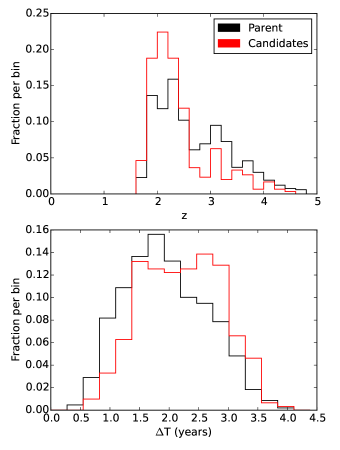
Figure 1: The distribution of redshifts (top) and rest-frame time between the spectra from SDSS and BOSS (bottom) for the parent sample (black) and the visually determined candidate emergent absorbers (red).

2.2 Gemini Observations

We obtained data on 105 targets from the candidate emergence sample using the twin Gemini telescopes. To select these 105 from the 306 visually identified to have emergent BAL activity, we prioritized targets which were candidates for non-BAL to BAL quasar transitions, targets with candidate C IV absorption at $v>30,000$ km s^-1, and brighter targets. At a given brightness, higher-redshift targets were preferred so that we could observe the entire 1200$-$1600 Å continuum and because of their shorter rest-frame times between the BOSS epoch and the proposed Gemini observations.

We used the Gemini Multi-Object Spectrograph (GMOS) (one on each telescope) outfitted with a 1.0^′′ wide longslit to observe individually each target in our sample. For the majority of our observations, we employed the use of the B600 grating with 600 lines mm^-1, a blaze wavelength of 461 nm, simultaneous wavelength coverage of $\sim$300 nm, and $R\sim 1688$. For some high-redshift targets, we used the R400 grating with 400 lines mm^-1, a blaze wavelength of 764 nm, a simultaneous wavelength coverage of $\sim$400 nm, and $R\sim 1918$. These settings were chosen such that the resulting data had similar spectral resolution to the SDSS/BOSS spectra. We set our exposure times to yield a signal-to-noise ratio of $\gtrsim$15 in the rest-frame 1200$-$1600 Å region. This was chosen to be equal to or higher than the signal-to-noise ratio found in SDSS and BOSS quasar spectra.

Our Gemini follow-up of the 105 targets was spread over three observing semesters: 2013A, 2013B, and 2014A. In total, we ran three different observing campaigns, each with multiple programs on either Gemini North or South. In Table 2 we list all observing program reference numbers, the number of quasars observed in that program, and some other notes. The main campaign was the initial follow-up observations, targeting all 105 quasars. A smaller, more specific program was initiated targeting BALs from the main campaign that exhibited variability in troughs at high-velocity (specifically, BALs blueward of Si iv emission). Finally, we were able to utilize a separate Gemini observing campaign (PhotoVariability) to gather more data on one target.

Table 2: A summary of all observing programs on Gemini. Gemini spectra are available upon request from the authors.

Program Reference	Objects	Telescope, semester, standard star
Main CampaignA
GN$-$2013A$-$Q$-$104	14	North, 2013A, HZ44
GS$-$2013A$-$Q$-$86	19	South, 2013A, LTT6248
GN$-$2013B$-$Q$-$59	15	North, 2013B, G191B2B
GS$-$2013B$-$Q$-$50	7	South, 2013B, LTT7379
GN$-$2014A$-$Q$-$67	24	North, 2014A, HZ44
GS$-$2014A$-$Q$-$24	27	South, 2014A, EG274
High Velocity CampaignB
GN-2014B-Q-75	3	North, 2014B, G191B2B
PhotoVariability CampaignC
GN-2013B-Q-39	1	North, 2013B, HZ44
GS-2013B-Q-21	1	South, 2013B, LTT7379

• The main observing campaign targeted all 105 targets. There are actually a total of 106 numbered above because object J161336 was observed both in GS$-$2013A$-$Q$-$86 and GN$-$2014A$-$Q$-$67.

• The high-velocity campaign gathered multiple spectra of 3 targets that were already observed in the main campaign: J073232, J083017, J083546.

• The aim of this spectroscopic followup campaign (see Rogerson et al. 2012) was only tangentially related to the science of this work; however, we were able to use the Standard Target of Opportunity feature of Gemini to observe J023011 twice.

In the top portion of Figure 2, the distribution of redshift is plotted for the original visually determined candidate sample (green) and those that were observed on Gemini (red). In the bottom portion of this plot the distributions of time between observations have been plotted, $\Delta T$. The red histogram is the $\Delta T$ values for the objects traced out by the red histogram in the top plot. The blue histogram is the rest-frame time between the most recent BOSS observation, and our Gemini follow-up observations. The cyan histogram represents a number of data sets, as follows: while our target selection was predicated on just one epoch from each of DR7, DR9, and DR10, there are many cases where there are multiple epochs from each data release for each target. Further, a small subset of our targets from the Main Campaign were observed again in other campaigns. The cyan histogram captures all rest-frame time between all successive spectral epochs available for a given target from DR7, DR9, DR10, and Gemini. See § 2.5 for a full summary of our observational data.

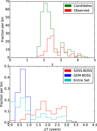
Figure 2: Top: The redshift distribution of the visually determined candidate sample (green), and the subset of those that received follow-up Gemini observations (red). Bottom: Rest-frame time separations between successive observations of targets that received follow-up observations on Gemini. The SDSS-BOSS histogram shows the successive-observation time separations of the last SDSS observation and the first BOSS observation of each quasar. The GEM-BOSS histogram shows the successive-observation time separations of the last BOSS observation and the first Gemini observation of each quasar. The Entire Set represents all successive-observation time separations in our dataset, including those involving additional archival epochs or Gemini observations. See Table 3 for further clarification.

2.3 Gemini Reductions

The Gemini spectra were reduced using the Gemini IRAF package created by the observatory, following standard techniques.

Only one set of standard star spectra was taken over the course of each observing program (one for each GMOS wavelength setting used in the program). Each star is listed in Table 2 and was taken from Landolt (1992). Due to the queue nature of our observations, this meant the calibration stars were not measured on the same night as the quasars themselves and could be separated in time by as much as 5 months. Thus, while we can use the standard stars to correct the shape of the quasar spectrum, they cannot be spectrophotometrically calibrated.

All SDSS and BOSS spectra have wavelength scales based on vacuum wavelengths. The Gemini wavelength calibrations are based on atomic transitions measured in air. In order to properly compare all data in this work, it was necessary to shift the Gemini spectra wavelength scale into the vacuum frame. The standard for this conversion is given in equation (3) of Morton (1991).

2.4 Normalizing the Spectra

Our data consist of at least three spectra from three different instruments attached to multiple telescopes. Moreover, for each quasar, observations could be separated by as much as a decade in the observed-frame. To compare easily the relative strengths of the absorption features in data from different telescopes and instruments, we normalized the spectra via the following approach.

In the rest-frame, the ultraviolet-optical continuum of a typical quasar can be modeled as a power law (to an acceptable approximation). Assuming all quasars are represented by this model, a power law can then be fit to the continuum of each quasar and divided out. The resulting normalized spectrum would then have the continuum resting at a unit-less normalized flux density of 1.0, any emission features would be greater than 1.0, and any absorption features would be less than 1.0.

To fit a power-law to the continuum, we chose normalization windows on the spectra that were relatively free of emission or absorption thus making these regions a clean sample of the continuum. Normalization windows for all 105 targets were chosen by eye with the goals of avoiding all absorption features and as many emission features as possible and of selecting regions available in all spectra of each target. In Filiz Ak et al. (2012), six relatively line-free regions were identified and used for normalization purposes: 1250$-$1350, 1700$-$1800, 1950$-$2200, 2650$-$2710, 2950$-$3700, and 3950$-$4050 Å. These regions were also identified in Vanden Berk et al. (2001) as being relatively clear of any emission features. Unfortunately, the Gemini spectra have much narrower wavelength coverage than the SDSS and BOSS spectra; hence, the Gemini spectra narrowed our selection of normalization windows. Most of the Gemini spectra extend only to $\sim$1750 Å.

It is important that all chosen normalization windows are the same for all epochs in a given quasar, so that we can be sure the continuum has been fit consistently in all data. As a result of this requirement, we are unable to use most of the line-free regions from other works mentioned above. A further result of the smaller wavelength coverage of the Gemini data is that we were forced to use normalization windows in the region where we are searching for absorption (i.e., between 1200$-$1550 Å), though as much as possible we chose normalization windows from the list above.

2.5 Tabular Summary of Observations

The complete list of 105 quasars observed in the Gemini campaigns is provided online in machine-readable format. In Table 3, we have provided a portion of the list to guide the reader. Each quasar is labeled by its SDSS DR7 name in the first column, though in this work we typically refer to each object by just the first half of that name. In the second column is the quasars redshift. The modified julian day (MJD) of the observations we collected from SDSS, BOSS, and Gemini are labeled in the columns thereafter. In our dataset, each quasar was observed at least three times, once from each of SDSS, BOSS, and Gemini. Many quasars were observed more often than that, with as many as two observations coming from SDSS, two coming from BOSS, and five from the Gemini observations, making a total of nine possible observations. In Table 3, if we have left a ‘-’ marking a position where no observations were made. In Table 4, the rest-frame time measured in days between successive observations for a given target is given. As for Table 3, only a portion of the table is provided, with the entire table availble online in machine-readable format.

Table 3: A list of the observations made for each of the 105 quasars in this work. The objects designation from SDSS DR7 is in the first column, and the MJDs of each observation are labeled thereafter. There were a maximum of two observations from SDSS, two from BOSS, and five from our Gemini campaigns, though not all objects had that many observations.

DR7 Designation	z	SDSS1	SDSS2	BOSS1	BOSS2	GEM1	GEM2	GEM3	GEM4	GEM5
022143.19$-$001803.8	2.65	51869.26	54081.18	55477.34	-	56654.10	-	-	-	-
022559.78$-$073938.8	3.02	51906.31	-	55832.86	-	56604.27	-	-	-	-
023011.28$+$005913.6	2.47	52200.39	52942.34	55208.64	55454.94	56519.53	56649.21	56685.07	-	-
073232.80$+$435500.4	3.46	53314.44	-	55180.31	-	56567.61	56924.60	56951.56	57006.41	57032.30
074711.14$+$273903.3	4.13	52592.49	52618.32	55536.28	-	56569.60	-	-	-	-
081114.66$+$172057.4	2.33	53357.32	-	55579.23	-	56327.49	-	-	-	-
081811.49$+$053713.9	2.52	52737.48	52962.51	55888.42	-	56594.60	-	-	-	-
082313.06$+$535024.0	2.56	53299.48	53381.75	55181.90	56748.12	56328.36	-	-	-	-
082801.67$+$411937.2	2.55	52265.88	54524.13	55513.42	-	56327.52	-	-	-	-
083017.31$+$413521.5	2.21	52265.88	54524.13	55513.42	-	56335.27	56956.58	57013.44	57046.33	-

Table 4: The rest-frame time between successive observations of a given quasar.

DR7 Designation	$\Delta$12	$\Delta$23	$\Delta$34	$\Delta$45	$\Delta$56	$\Delta$67	$\Delta$78	$\Delta$89
022143.19$-$001803.8	606.74	382.97	322.79	-	-	-	-	-
022559.78$-$073938.8	975.73	191.69	-	-	-	-	-	-
023011.28$+$005913.6	213.63	652.55	70.92	306.53	37.34	10.32	-	-
073232.80$+$435500.4	418.18	310.93	80.01	6.04	12.29	5.8	-	-
074711.14$+$273903.3	5.04	568.99	201.5	-	-	-	-	-
081114.66$+$172057.4	667.38	224.75	-	-	-	-	-	-
081811.49$+$053713.9	63.87	830.49	200.44	-	-	-	-	-
082313.06$+$535024.0	23.13	506.06	322.3	118.01	-	-	-	-
082801.67$+$411937.2	636.10	278.66	229.31	-	-	-	-	-
083017.31$+$413521.5	703.39	308.14	255.98	193.52	17.71	10.25	-	-

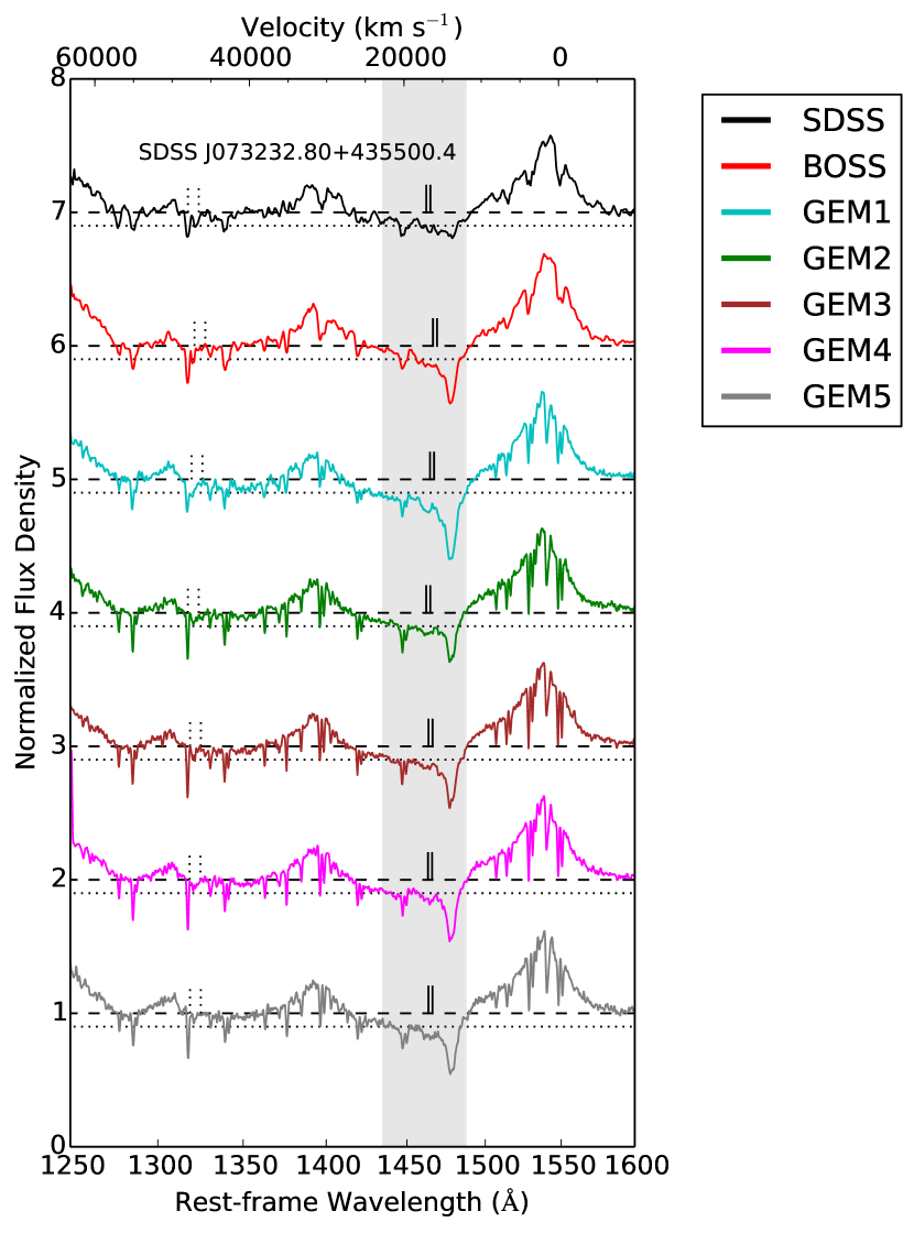
Figure 3: All spectra gathered for SDSS J073232.80$+$435500.4 are plotted in this figure. The rest-frame wavelength in Angstroms (Å) is on the bottom x-axis. The top x-axis displays the outflow velocity in km s^-1 relative to the systemic redshift of the quasar, as measured from the C iv emission feature at ∼1550 Å. The y-axis is normalized Flux Density units. Each spectrum available for this quasar is plotted, artificially separated in the y-direction to make comparisons between epochs easier. For each spectrum, there is a dashed line placed at the normalized continuum level, and a dotted line placed at 90% of the normalized continuum level. The spectrum with the smallest MJD is at the top, and each successive epoch in chronological order is placed below. The colors represent different data, which is given in the legend. In each spectrum, the centroid velocity of each absorption complex is denoted by two small vertical black bars, which represent the C iv doublet at $\lambda$$\lambda$ 1548.202,1550.774 Å. The expected locations of Si iv absorption that could accompany each C iv doublet are denoted by two small vertical dashed lines, which represent the Si iv doublet at $\lambda$$\lambda$ 1393.755,1402.770 Å. This is an example plot. A plot for all 105 quasars in this study is available in the electronic version of this publication.

2.6 Signal-to-Noise and Smoothing

Our data show a range of SNR for each spectral epoch due to the observations’ different telescopes, instruments, and observing conditions. To compare these spectra properly, we applied the following smoothing routine. We measure SN₁₅₀₀, the median (flux density)/(1$\sigma$ noise) value for all pixels at $1400-1600$ Å, and determine which spectrum has the highest SN₁₅₀₀ for the quasar. Each other spectrum of this quasar is smoothed with a boxcar filter an odd number of pixels wide, using the smallest number that yields SN₁₅₀₀ at least equal to highest SN₁₅₀₀ found for the quasar. To avoid degrading the effective resolution of the spectra, we capped the boxcar width at 9 pixels.

2.7 Identification of Broad Absorption Lines

The targets selected in § 2.1 were found by visual identification of emergent broad absorption (see § 2.1 for details). This was a satisfactory approach to determine an initial set of quasars to study but did not include a formal definition of absorption that confirmed the visual emergence as statistically significant absorption. A formal definition that would cleanly separate quasars into those with broad absorption lines (BAL quasars) and those without (non-BAL quasars) is required in order to reduce subjectivity and allow comparison of the trough strength in BAL quasars.

In response to this need, Weymann et al. (1991) defined the BALnicity Index (BI). The original definition of the BI measured the amount of absorption (in units of km s^-1) of C iv by integrating over all available absorption troughs in a spectrum while applying the following criteria. Any absorption that is included in the index must be at least 2,000 km s^-1 wide; any absorption found within the first 3,000 km s^-1 blueward of the C iv emission peak (at $\sim$1550 Å) is ignored; no absorption after 25,000 km s^-1 blueward of the C iv emission peak is included; and, the flux density in the trough must be below 90 % of the normalized flux density at the continuum.

As research into BAL quasars progressed, it was realized that this original definition of BALnicity erred on the conservative side; it does not fully encompass all intrinsic broad absorption observed in quasar spectra. For example, a trough narrower than the 2,000 km s^-1 criterion can still be rooted in the same physical origin as broader troughs and should be included. These are known as ‘mini-BAL’ troughs in the literature and range in width from 500$-$2,000 km s^-1 (e.g., Rodríguez Hidalgo et al. 2011). Modifications of the BALnicity Index have been proposed (e.g., Hall et al. 2002; Trump et al. 2006) to include absorption over wider velocity ranges.

For this work, in which we are interested in troughs which may be narrower or at higher outflow velocities (or both) than considered in the traditional BI definition, we measure BALnicity using a modification of the index proposed in Trump et al. (2006), which we define as:

$${\rm BI}^{*}=\int_{v_{low}}^{v_{high}}\left(1-\frac{f(v)}{0.9}\right)C_{1000}~{}dv,$$ (2)

using the asterisk to distinguish it from the original BI definition. In the above, $f(v)$ is the normalized flux density at a given velocity and the quantity $C_{1000}$ is equal to 1 only in regions more than 1,000 km s^-1 wide in which the quantity in parentheses is everywhere greater than zero, otherwise it is set to 0. That change is similar to Trump et al. (2006). In the above equation, $v_{low}$ and $v_{high}$ are purposefully not defined to indicate there is no formal limit on the minimum and maximum absorbing velocities. (A minimum velocity of zero would exclude the rare but interesting redshifted-trough BAL quasars; see Hall et al. 2013). In § 2.1, targets with possible absorption anywhere between the Ly$\alpha$ emission and C iv emission were chosen. Historically, the region betwen Ly$\alpha$ and Si iv emission lines was excluded because this region could be contaminated by Si iv absorption associated with C iv absorption. This is why the original BALnicity measurements were capped at 25,000 km s^-1 blueward of the C iv emission peak. We specifically searched for absorption from C iv in both the classically searched velocity regimes, but also in much higher velocities regimes. Thus, while no formal limits on the BALnicity were required for this work, in practice the bounds on BI^∗ were set to $0<v~{}(\textrm{km~{}s${}^{-1}$})<$ 65,000. If BI^∗$>0$ we consider there to be statistically significant absorption present; a BI^∗$=0$ indicates no absorption is present. After absorption is identified, we then determined if the absorption was a result of high-velocity C iv or accompanying Si iv (see Fig. 3, and the next section, for this identification).

2.8 Measurement of BAL Trough Properties

All normalized spectra were run through an automatic BALnicity measurement routine. As part of this routine, on top of the variable smoothing from § 2.6 we smoothed by an additional 3-pixel-wide boxcar to implement Savitsky-Golay smoothing, which weights pixels closer to the centre of the smoothing window more than those at the edge of the window (see Savitzky & Golay 1964).

All absorption meeting the BI^∗ requirements identified by the measurement routine was visually inspected, and any contamination was removed. There were a number of possible contaminants that required visual confirmation or elimination. Intervening absorption or narrow C iv systems are, by design, meant to be ignored by BI^∗. However, narrow systems in spectra that were heavily smoothed by our technique were sometimes smoothed out enough in velocity to be falsely detected as BAL troughs; such cases were removed by comparing the smoothed spectrum to the un-smoothed spectrum after the absorption had been identified. Narrow systems may also occur on-top or blended into a BAL feature. If this occurred, the contribution of the narrow system was included in the measurement of BI^∗. While this means there are some possible contaminations for the individual BI^∗ numbers, it is important to note that this paper focuses on the difference in absorption from one epoch to another. Assuming the narrow systems have remained relatively constant over our observation campaigns, their effects would cancel out in calculating change in absorption. We also removed Si iv BAL troughs accompanying C iv troughs. Quasar-specific details regarding how contaminations were dealt with can be found in that quasar’s individual caption in the online figure set; see Fig. 3.

After all non-C iv-BAL related detections were removed, there were a total of 653 individual C iv absorption troughs across all 360 normalized spectra in the 105 quasars. To quantify the properties of this sample of absorption troughs, we measured each trough’s centroid velocity (in km s^-1), width (in km s^-1), and fractional depth below the normalized continuum in two ways detailed in the next paragraph. The centroid velocity, $v_{cent}$, of a trough was measured following the definition in Filiz Ak et al. (2013): the mean of the velocity in a trough where each pixel is weighted by its distance from the normalized continuum. The width of a trough is the velocity range over which the trough met the BI^∗ criteria.

The mean depth of the trough was calculated in two ways. First, we measured $d_{BAL}$ as in Filiz Ak et al. (2013), which is the mean depth of the trough relative to the normalized continuum of 1.0 for each data point in the trough. Second, we measured $d_{max7}$, a measure of the maximum trough depth which is calculated by sliding a 7-pixel-wide window across the trough, measuring the average depth over each window relative to the normalized continuum at 1.0, and taking the largest depth over all these windows as $d_{max7}$. The uncertainty on the depth is calculated as the uncertainty in the mean of the 7 pixels in the average. We note that since the observations were taken with different telescopes and instrument set ups, 7 pixels correspond to slightly different resolutions; however, the differences do not substantially affect the results.

The distribution of trough width versus trough centroid velocity is plotted in Figure 4. The mean centroid velocity in the plot is 19,500 km s^-1, and the mean trough width is 3,600 km s^-1. The widest trough, at 22,200 km s^-1, was observed in J083546; its spectra are plotted in § 4.6. There are noticeable gaps in the centroid velocity distribution at 30,000 km s^-1 due to Si iv emission at $\sim 1400$ Å, at 43,000 km s^-1 due to C ii emission at $\sim 1335$ Å, and at 50,000 km s^-1 due to Si ii+O i emission at $\sim 1304$ Å. Si iv is on average the strongest of those three lines in terms of emission-line equivalent width and C ii is the weakest (Vanden Berk et al., 2001). Correspondingly, the gap in the distribution of centroid velocities is widest for Si iv and narrowest for C ii. The presence of broad emission either raises the flux density level from which absorption must remove flux or adds flux density which does not pass through the absorber on its way to us. Either case can make it more difficult for the deepest part of the trough from a given absorber to drop below our detection threshold of 0.9 times the continuum level. Thus, while there is likely absorption present at these velocities, only the strongest absorption is detected.

The distribution of trough depth (both $d_{BAL}$ and $d_{max7}$) versus trough centroid velocity is plotted in Figure 5. The quantity $d_{max7}$ measures the maximum depth of the trough, and indeed measures on average larger depths than $d_{BAL}$, which is representative of the mean depth over the entire trough. In black is $d_{BAL}$, with a mean value of 0.24, and in red is $d_{max7}$ with mean 0.32. The $d_{max7}$ value at $0.6$ and approximately 57,000 km s^-1 is from object J105210 and is the result of an intervening absorber sitting on top of a BAL at high velocity.

In Figure 6, the trough width is plotted against the BI^∗ of each trough. The mean BI^∗ is 678 km s^-1. The largest value of BI^∗ is found in J130600. In its BOSS spectrum, the absorption spans the entire region between C iv and Si iv emission, reaches $d_{BAL}=0.4$, and width of 17,600 km s^-1. It is the second-widest trough, next to J083546 above.

Finally, the trough depth (both $d_{BAL}$ and $d_{max7}$) is plotted against trough width in Figure 7. The two data points at very high trough width are a result of J083546. Again, in this case $d_{max7}$ is not the best measure of the depth of the trough because it is biased by a narrow feature sitting on top of the broad absorption.

Figure 4: The distribution of trough widths and trough centroid velocities for all absorption identified by the BI^∗ criteria. There are a total of 653 absorption features in 360 spectra. The gaps near 30,000 and 50,000 km s^-1 centroid velocity are due primarily to absorption at wavelengths overlapping Si II or Si IV emission not reaching the detection threshold of 10 % below the level of the power-law continuum.

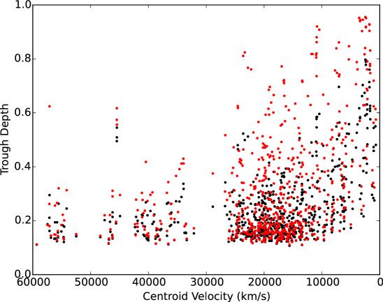
Figure 5: Comparing the depth of troughs relative to the normalized continuum at 1.0, versus their centroid velocities for all absorption identified by the BI^∗ criteria. There are a total of 653 absorption features in 360 spectra. The black points are $d_{BAL}$, and the red points are $d_{max7}$.

Figure 6: The BI^∗ plotted against the width of the troughs identified by the BI^∗ criteria.

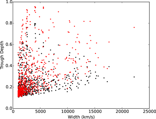
Figure 7: The depth $d_{max7}$ (red) and $d_{BAL}$ (black), relative to the continuum at 1.0, plotted against the velocity width of the trough.

3 Methods

3.1 Absorption Complexes

From epoch to epoch, a given trough may split into multiple smaller troughs as it decreases in absorption strength, or two adjacent smaller troughs may merge into one large trough as the absorption of one or both of the troughs widens, or the depth increases. In order to characterize properly the variability of broad absorption between epochs, we identify BAL complexes. We have mimicked the approach of Filiz Ak et al. (2013) in identifying complexes. In Figure 8, we show an example of how this an absorption complex is identified for the quasar J082313. In the earliest epoch, no absorption feature is observed. In the following epoch a large trough emerges, spanning the region $1411.2-1475.3$ Å. In the final epoch, that large trough has split into two separate troughs spanning $1420.4-1426.0$ Å and $1439.4-1466.9$ Å. We consider this all to be one complex of C iv absorption. To identify complexes, we follow these steps:

1. Sort all troughs identified by the BALnicity code above in order from highest velocity to lowest. They are also sorted into spectral epoch order, from oldest to newest observations.

2. Begin with the highest velocity trough in the oldest spectrum, setting the $v_{max}$ and $v_{min}$ of the absorption complex to this trough’s velocity range values.

3. Loop through all absorption features in the following epochs. If the complex’s $v_{max}$ intersects a trough in a later epoch, reset $v_{max}$ to that trough’s $v_{max}$. The same is done for $v_{min}$.

4. This is repeated for all absorption features identified by the BALnicity measurements above.

5. Repeat the entire process starting with the most recent epoch and moving toward the oldest. This step ensures that troughs in the velocity range of the complex are counted as part of the complex in all epochs.

As is evident in Figure 8, this procedure results in a maximum and minimum velocity, $v_{max}$ and $v_{min}$, respectively, range that encompasses all absorption that overlaps in that region for all epochs; we define the difference between these two values as the velocity width of the absorption complex. Thus each of the 653 individual C iv absorbers are associated with one complex. This results in 219 individual absorption complexes across all 105 quasars in our sample.

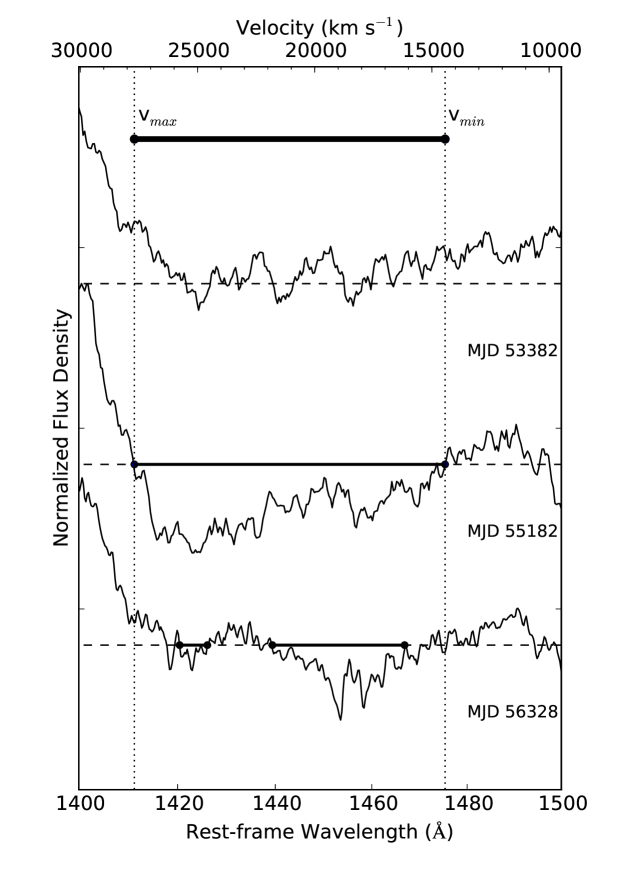
Figure 8: This figure demonstrates an example of how an absorption complex is identified and measured. The Spectra is of quasar J082313.06$+$535024. The oldest spectral epoch is at the top, and each epoch is in chronological order after that (see the MJD label beside each spectrum). In all epochs, part of the Si IV emission line is seen just longward of 1400 Å. In the first epoch, there is no absorption, in the second a broad absorption trough appears, and in the final epoch, that trough splits into two. The thin black lines indicate the individual absorption features, and the entire absorption complex identified by the prescription in § 3.1 is labeled at the top from $v_{max}$ to $v_{min}$. Note, that while there are varying numbers of individual troughs for each epoch, it is considered to be one complex.

3.2 Quantifying the Absorption

In order to quantify the variability in the absorption complexes identified in the previous section, we must measure some of their absorption parameters. After absorption complexes have been identified in the spectra, we measured the equivalent width (EW; in Å, defined below), the weighted centroid velocity $v_{cent}$, and the average trough depth ($d_{BAL}$ and $d_{max7}$) over that region for all epochs of a quasar’s spectrum. This is regardless of whether or not absorption is actually identified in the spectrum. For example, in Figure 8, the earliest spectral epoch at MJD 53382 exhibits no absorption, however, we still measure the EW, $v_{cent}$, and depth of the trough over the complex’s range in this epoch. This provides us with a baseline from which to measure changes.

To measure the EW in Å and its uncertainty from the normalized spectra we used equations 1 and 2 of Kaspi et al. (2002):

$$\textrm{EW}=\sum_{i}\left(1-\frac{F_{i}}{F_{c}}\right)B_{i},$$ (3)

and,

$$\sigma_{\textrm{EW}}=\sqrt{\left[\frac{\Delta F_{c}}{F_{c}}\sum_{i}\left(\frac{B_{i}F_{i}}{F_{c}}\right)\right]^{2}+\sum_{i}\left(\frac{B_{i}\Delta F_{i}}{F_{c}}\right)^{2}}.$$ (4)

$F_{i}$ and $\Delta F_{i}$ are the normalized flux density and its error in the $i$th bin. $F_{c}$ and $\Delta F_{c}$ are the mean and the uncertainty on the mean of the continuum normalized flux density measured in the normalization windows. $B_{i}$ is the bin width in units of Å. In our normalized spectra, $F_{c}=1$ and $\Delta F_{c}$ values are calculated using the normalization windows determined by the normalization procedure in § 2.4. Thus $\sigma_{\textrm{EW}}$ represents the statistical uncertainty inherent in spectra. It does not quantify the systemic uncertainty, which is governed by the placement of the continuum by normalization. The wavelength range over which the sums in equations (3) and (4) are measured is set by the identification of $v_{max}$ and $v_{min}$ in the previous section. The BI^∗ is measured only when the normalized flux density is below 90 % of the total continuum for more than 1000 km s^-1. The beginning and ending wavelengths where this criterion is satisfied are carried over to the absorption complexes, and the EW is measured between them. Thus, while the range over which equations (3) and (4) are measured is set by this criterion, we still use $F_{c}=1$ as the normalized continuum level (and not 0.9 as might have been expected).

As mentioned in § 2.8, we use the centroid velocities and mean depths as tool to compare troughs. We now apply the same measurements to the velocity range of the absorption complexes with a caveat in the case of measuring the centroid velocity. If in the absorption complex, the normalized flux density is above 1.0, the velocity of that bin is not counted toward the weighted mean $v_{cent}$. If all of the normalized flux density is above 1.0 for the absorption complex, which can happen in cases where absorption has disappeared on top of an emission feature, then all bins are weighted equally. This results in a centroid velocity being in the mean of the absorption complex’s maximum and minimum velocities. Calculating the mean depths, $d_{BAL}$ and $d_{max7}$, in the absorption complex is the same as in § 2.8, i.e., the normalized flux density values above 1.0 are not ignored.

3.3 Measuring Variability

There are several ways to compare one epoch to the next for any of the absorption complexes. We adopt several methods including the measurement of change of EW:

$$\Delta\textrm{EW}=\textrm{EW}_{2}-\textrm{EW}_{1}\qquad\sigma_{\Delta\textrm{EW}}=\sqrt{\sigma^{2}_{\textrm{EW}_{2}}+\sigma^{2}_{\textrm{EW}_{1}}}.$$ (5)

We also measure the fractional change in EW, which is the change in EW from one epoch to the next divided by the average EW over both epochs (e.g, Ganguly & Brotherton 2008, Filiz Ak et al. 2013). This measurement indicates how significant a change in absorption is compared to the size of the feature that is changing.

$$\frac{\Delta\textrm{EW}}{\langle\textrm{EW}\rangle}=\frac{\textrm{EW}_{2}-\textrm{EW}_{1}}{(\textrm{EW}_{2}+\textrm{EW}_{1})\times 0.5}$$ (6)

$$\frac{\sigma_{\Delta\textrm{EW}}}{\langle\textrm{EW}\rangle}=\frac{4\times(\textrm{EW}_{2}\sigma_{\textrm{EW}_{1}}+\textrm{EW}_{1}\sigma{\textrm{EW}_{2}})}{(\textrm{EW}_{2}+\textrm{EW}_{1})^{2}}$$ (7)

Similarly, we measure the change in depth from one epoch to the next, and those corresponding uncertainties:

$$\Delta d_{BAL}=d_{BAL,2}-d_{BAL,1}$$ (8)

$$\sigma_{\Delta d_{BAL}}=\sqrt{\sigma^{2}_{d_{BAL,2}}+\sigma^{2}_{d_{BAL,1}}}.$$ (9)

$$\Delta d_{max7}=d_{max7,2}-d_{max7,1}$$ (10)

$$\sigma_{\Delta d_{max7}}=\sqrt{\sigma^{2}_{d_{max7,2}}+\sigma^{2}_{d_{max7,1}}}.$$ (11)

These diagnostics of variability are calculated between all epochs for all 219 absorption complexes in the dataset.

4 Results and Discussion

4.1 Summary of Absorption Complex Characteristics

Combining BI^∗ requirements with the absorption complex identification routine resulted in 219 individual C iv absorption complexes in 105 quasars. Of the 105 quasars in our dataset, two quasars, J121314 and J142903, did not end up having any absorption that met the BI^∗ criteria for absorption, making the total number of quasars that contributed data for absorption complexes to this study 103. Both J121314 and J142903 are still included in the observation Tables 3 and 4, and the online figure set (Fig 3) for completeness data was collected for them using Gemini. There are a total of 354 spectra for these 103 quasars, as each quasar is observed between 3-7 times (see Table 3).

The distribution of maximum and minimum velocities, $v_{max}$ and $v_{min}$, respectively, in the 219 absorption complexes is plotted in Figure 9. The quasar with the largest $v_{max}$ was J023011 with 59,800 km s^-1. The smallest $v_{max}$ was found in J091621 at 1,400 km s^-1, which also had the smallest $v_{min}$ at just 30 km s^-1. The largest $v_{min}$ is at 58,800 km s^-1 in quasar J113536.

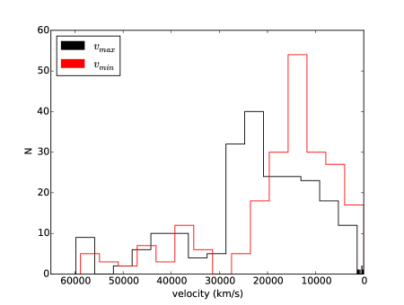
Figure 9: The distribution of absorption complex maximum and minimum velocities, $v_{max}$ and $v_{min}$, respectively. The majority of the values are between 0 and 30,000 km s^-1, the region between C iv and Si iv. The distributions nonetheless extend to the largest velocities probed.

We plot the distribution of absorption complex velocity widths, which was defined in § 3.1, in Figure 10. There are more complexes with smaller widths than with large widths. The widest absorption complex is found in J165642; it contains a complex 24,600 km s^-1 wide. The smallest absorption complex width in our sample is 1,000 km s^-1, which is the lower limit imposed by the BI^∗ criterion. Note that the widths presented in Figure 10 are not the true widths of individual troughs, but the widths of the complexes.

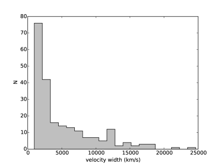
Figure 10: The distribution of absorption complex velocity width. There are 219 data points in the histogram. The figure shows that most of the troughs have small widths, peaking well below the 5,000 km s^-1 value. Note that the smallest allowable width was 1,000 km s^-1.

The distribution of absorption complex centroid velocities, $v_{cent}$, is plotted in Figure 11. There are 219 absorption complexes, each complex having at least 3 epochs of observations; this results in 748 data points.

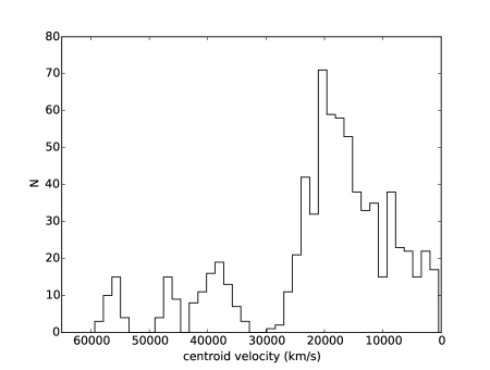
Figure 11: The distribution of absorption complex centroid velocities, $v_{cent}$. There are 748 data points in the histogram. The majority of the centroid values lie between 0 and 30,000 km s^-1, the region between C iv and Si iv. Also of note in the figure is the lower number of troughs identified at the wavelengths of various emission features: Si ii at $\sim$50,000 km s^-1, C ii at $\sim$45,000 km s^-1, and Si iv at $\sim$30,000 km s^-1.

In Figure 12, for every complex the centroid velocity is plotted against the width. There is a marked absence of troughs wider than 10,000 km s^-1 beyond the wavelength of Si iv at $\sim$30,000 km s^-1.

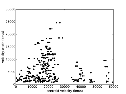
Figure 12: The width of the absorption complexes versus the individual centroid velocities measured for each epoch. There are 748 data points plotted.

4.2 BAL/non-BAL Transitions

An emergent BAL quasar is defined as a quasar which is measured to have BI^∗$=0$ in one spectral epoch and BI^∗$>0$ in the next spectral epoch. This change indicates that a significant trough appeared in a quasar which was previously designated a non-BAL quasar. Of course, the opposite can happen: all troughs in a BAL quasar can disappear and change the quasar’s designation from BAL to non-BAL. Such objects were studied extensively in Filiz Ak et al. (2012).

Of the 103 targets with significant absorption in our dataset, there were 36 instances of transition from non-BAL to BAL: emergent BAL quasars. In all but three of these instances the transition occurred between the SDSS and BOSS observations, which is expected given that the full sample was chosen due to visual identification of new absorption between those epochs. The remaining three transitions occurred in J113536, J145230, and J222838 between their BOSS and Gemini observations. In these quasars, emergent absorption is visible in the SDSS-BOSS transition but it did not meet the BI^∗ criterion. However, the visually identified emergence continued to increase into the Gemini observation, where it became strong enough (in all three quasars) to be considered a BAL trough.

There were 11 cases in our sample of a quasar transitioning from BAL to non-BAL, occurring in 10 different quasars (the quasar J015017 made this transition twice; see below). Seven of these cases occurred in the BOSS-Gemini transition, two in the SDSS1-SDSS2 transition, and two in the SDSS-BOSS transition. The two cases of occurrence in the SDSS-BOSS transition were in J132508 and J150935, and the spectrum of the former is shown in § 4.6.

There were 5 quasars that exhibited both emergence and disappearance over the course of our observations: J015017, J022143, J081811, J095254, and J142054; these objects have behavior similar to SDSS J093620.52+004649.2 (Filiz Ak et al., 2012; Lundgren et al., 2007). Of particular interest was quasar J015017; its spectra are plotted in Figure 13. In the 101.25 days between SDSS1 and SDSS2 observations, all BAL troughs disappeared in J015017. The troughs reappeared with a much stronger absorption 745.54 days later in the BOSS1 observation. Between BOSS1 and BOSS2 (66.41 days) the trough weakened substantially. Finally, the troughs disappeared again in the Gemini observation, 303.05 days after the last BOSS observation.

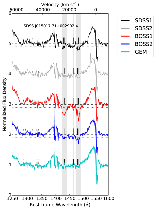
Figure 13: A plot of spectra taken at five different epochs for the quasar J015017. Note the changes in the three absorption complexes in the wavelength range 1400 Å to 1500 Å. With the first spectrum at the top, and each successive observation in chronological order below, we can observe these complexes emerge between the 2nd and 3rd observation, then disappear again between the 4th and 5th.

4.3 BAL Quasar Emergence and Disappearance Rates

The candidate BAL trough emergence rate at $z>1.68$ for DR7$-$DR9 was $111/7417=1.50\pm 0.14$ %, and for DR7$-$DR10 was $181/8239=2.20\pm 0.17$ %. These rates differ by 3.2$\sigma$ when only Poisson noise is considered in the uncertainties. Additional uncertainties in the rates can arise due to signal-to-noise-dependent identification of troughs, for example, so we consider the rates from the two subsamples to be consistent when all sources of uncertainty are considered. Combined, we find a BAL trough emergence rate at $z>1.68$ of $292/15656=1.87\pm 0.11$ % over the rest-frame timescales of $1-3$ years separating DR7 and DR9+DR10.

The rate at which non-BAL quasars transitioned to BAL quasars is lower, as many BAL troughs appeared in pre-existing BAL quasars. From the previous section, 33 non-BAL to BAL transitions occurred between SDSS and BOSS among 103 visually identified candidates followed up with Gemini spectra, a fraction of $32\pm 6$ %. Thus, we find a non-BAL to BAL quasar emergence rate of $R_{E}=0.59\pm 0.12$ % at $z>1.68$ over rest-frame timescales of $1-3$ years.

In equilibrium, the BAL emergence and disappearance rates $R_{E}$ and $R_{D}$ and the numbers of BAL and non-BAL quasars $N_{B}$ and $N_{N}$ in the parent sample are related by $R_{E}N_{N}=R_{D}N_{B}$, or $R_{E}=R_{D}(N_{B}/N_{N})$.

In Filiz Ak et al. (2012), 21 C iv broad absorption features were observed to disappear in 19 quasars selected from a parent sample of 582 BAL quasars in SDSS and BOSS. In 10 of those cases the quasars transformed from BAL to non-BAL, for a rate of $R_{D}=1.7^{+0.7}_{-0.5}$ % of BAL quasars disappearing (transforming into non-BAL quasars) over SDSS-BOSS timescales.

Using the above values for $R_{D}$ and $R_{E}$, we find $R_{E}/R_{D}=N_{B}/N_{N}=0.35^{+0.12}_{-0.16}$. That BAL to non-BAL quasar ratio $r\equiv N_{B}/N_{N}$ corresponds to a BAL quasar fraction in the parent sample of $f_{BAL}=r/(1+r)=0.26^{+0.09}_{-0.12}$. That value is consistent within the uncertainties with the incompleteness-corrected BAL quasar fraction of $f_{BAL}=0.140\pm 0.016$ found by Allen et al. (2011) at $z\geq 1.5$ in the SDSS. However, their smaller observed value of $f_{BAL}$ predicts a smaller emergence/disappearance ratio of $r=R_{E}/R_{D}=f_{BAL}/(1-f_{BAL})=0.16\pm 0.02$; in other words, either a lower emergence rate than we observe or a higher disappearance rate than observed in Filiz Ak et al. (2012), or both. Nonetheless, our BAL quasar emergence rates and the BAL quasar disappearance rates of Filiz Ak et al. (2012) are in agreement within the uncertainties.

4.4 Changes in Equivalent Width

With 103 quasars with 219 absorption complexes, and at least 3 observations per quasar, there are 526 epoch-to-epoch changes in EW, depth, and centroid velocity. In that set of data, 462 of the changes were statistically significant at greater than 3$\sigma_{\textrm{EW}}$, while the other 64 were within the noise. Thus, the fraction of absorption complexes that exhibited a statistically significant change in EW was 462/526=88$\pm$4 %, and no change was 64/526=12$\pm$1 %. Of course, this is biased because we specifically chose quasars to observe that showed some obvious changes in their spectra between the first two observations.

We plot the change in EW between successive epochs of all absorption complexes in the top portion of Figure 14 (see equation 5), and the fractional change in the bottom portion (see equation 7). All of the grey points in both figures are values taken from the literature (see Table 1). The colored points are from this work: black points represent changes between two SDSS observations, red points are changes from SDSS to BOSS observations, blue are changes between two BOSS observations, cyan are changes from BOSS to Gemini observations, and all other colors are changes between two Gemini observations. We note that our data largely traces the results of other works: on longer time-scales, large changes in EW are possible. There are no large changes in EW on short time-scales. Figure 14 also shows how our dataset has filled in the region on medium time-scales of $0.5-1.0$ years in the rest-frame, a region of parameter space that has been largely unexplored. Both absolute and relative EW change measurements are useful. The quantity $\Delta$EW/$\langle$EW$\rangle$ directly identifies BAL emergence ($\Delta$EW/$\langle$EW$\rangle$ = 2) and disappearance ($\Delta$EW/$\langle$EW$\rangle$ = $-2$). BAL emergence can occur on timescales as short as 0.2 rest-frame years, but only relatively small $\Delta$EW values are observed on such timescales. On timescales longer than 1 rest-frame year, our SDSS-BOSS comparisons (red points) show a larger range of both absolute and relative EW changes but are not dominated by cases of pure emergent troughs. Instead, strengthening troughs with the full range of positive $\Delta$EW/$\langle$EW$\rangle$ values are observed.

In Figure 15, the change in depth of trough is plotted against the time between successive observations as measured by $d_{BAL}$ (top) and by $d_{max7}$. Both figures display a similar trend of EW changes with time: on longer time-scales, larger changes are possible. The similarity between Figure 15 and Figure 14 is due to the fact that most EW variability is dominated by changes in trough depth rather than by changes in trough width.

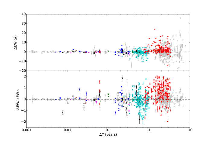
Figure 14: The change in equivalent width, $\Delta$EW, (top) and change in fractional equivalent width, $\Delta\textrm{EW}/\langle\textrm{EW}\rangle$, between successive epochs in a quasar as a function of rest-frame time between them. The grey points are taken from the literature (see Table 1). All other points are from this work. Black points represent changes between two SDSS observations, red points are changes from SDSS to BOSS observations, blue are changes between two BOSS observations, cyan are changes from BOSS to Gemini observations, and all other colors are changes between two Gemini observations.

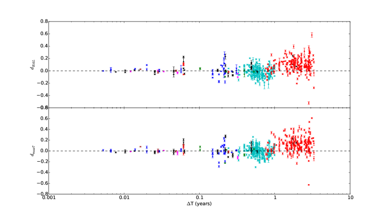
Figure 15: The change in $d_{BAL}$ (top) and $d_{max7}$ (bottom) between successive epochs in a quasar as a function of rest-frame time between observations. Black points represent changes between two SDSS observations, red points are changes from SDSS to BOSS observations, blue are changes between two BOSS observations, cyan are changes from BOSS to Gemini observations, and all other colors are changes between two Gemini observations.

4.5 Comparison of BAL quasars with and without emergent troughs

To study the properties of pre-existing BAL quasars and emergent BAL quasars in our DR7-DR9 and DR7-DR10 samples, we matched our samples with the SDSS DR12 BAL quasar catalog (Pâris et al., 2017), hereafter referred to as DR12QBAL. The DR12QBAL catalog consists of automated detections and measurements of BAL troughs in each DR12 quasar visually identified as having BAL features in its highest-SNR BOSS spectrum.

The DR12QBAL catalog measurements include the traditional balnicity index, here denoted $\rm BI_{\rm 2000}$:

$${\rm BI_{\rm 2000}}=\int_{3000}^{25000}\left(1-\frac{f(v)}{0.9}\right)C_{2000}~{}dv,$$ (12)

where $C_{2000}=1$ when the quantity in parentheses for a candidate trough is positive for more than 2000 km s^-1. The DR12QBAL catalog also includes the absorption index (Hall et al., 2002):

$${\rm AI_{\rm 450}}=\int_{0}^{25000}\left(1-\frac{f(v)}{0.9}\right)C_{450}~{}dv,$$ (13)

where $C_{450}=1$ when the quantity in parentheses for a candidate trough is positive for more than 450 km s^-1.

For each visually identified BAL quasar, the DR12QBAL catalog contains total $\rm BI_{\rm 2000}$ and $\rm AI_{\rm 450}$ values and the number of $\rm BI_{\rm 2000}>0$ and $\rm AI_{\rm 450}>0$ troughs; for each trough, velocity limits, maximum depths, and maximum depth velocities are given. DR12QBAL does not contain the $\rm BI_{\rm 2000}$ and $\rm AI_{\rm 450}$ values of the individual troughs in each object. We estimated those values as follows. We estimated the relative EW of each trough as the product of its velocity width times its maximum depth, divided by the sum of those products for all troughs in each object. While the individual EWs are clearly overestimates, the relative EWs are our best estimates of the relative strength of each trough. We multiply each trough’s relative EW by the total $\rm BI_{\rm 2000}$ or $\rm AI_{\rm 450}$ of the quasar to each trough’s estimated $\rm BI_{\rm 2000}$ or $\rm AI_{\rm 450}$.

From our DR7-DR9 sample of 8317 quasars at $z>1.68$, we find 1162 DR7-DR9 quasars in DR12QBAL for which measurements are available on the same BOSS spectra, including 77 of our emergent BAL quasar candidates.

From our DR7-DR10 sample of 8239 quasars at $z>1.68$, we find 1334 DR7-DR10 quasars in DR12QBAL for which measurements are available on the same BOSS spectra, including 99 of our emergent BAL quasar candidates.

We chose not to compare our DR9-DR10 quasar sample with DR12QBAL, because of the significantly shorter timescales between the first two epochs in that sample. This exclusion only affects five quasars with Gemini spectra.

We therefore have information from DR12QBAL on 176 emergent BAL quasar candidates, including 51 with Gemini spectra, and 2320 non-emergent BAL quasars.

There are 116 emergent BAL quasar candidates with absorption undetected in DR12QBAL, including 49 with Gemini spectra. Approximately half of those 49 non-detections are due to the emergent BAL trough being at a velocity $>$ 25000 km s^-1. The rest are a roughly equal mixture of shallow and narrow troughs. The differences between the catalogs in their common velocity range could be due to differences in continuum fitting, smoothing before BAL detection, and visual inspection of BOSS spectra alone for DR12QBAL as opposed to visual inspection of DR7 and BOSS spectra simultaneously for our catalog.

Next, in the 51 Gemini targets also found in the DR12QBAL catalog, we attempted to match our trough complexes with DR12QBAL troughs with $\rm BI_{\rm 2000}>0$. We chose to study matches with $\rm BI_{\rm 2000}>0$ troughs because our 1000 km s^-1 minimum trough width means we should detect all such troughs, but not all troughs with $\rm AI_{\rm 450}$. In this matching, we identified all $\rm BI_{\rm 2000}>0$ troughs overlapping in velocity with one of our trough complexes as part of that trough complex. We calculated the $\rm BI_{\rm 2000}$ value, velocity width, maximum depth, and velocity of maximum depth for each trough complex.

Only one trough with $\rm BI_{\rm 2000}>0$ in the 51 Gemini targets also found in the DR12QBAL catalog did not have a counterpart among our trough complexes. It is a trough in J123404 on the shoulder of the C iv broad emission line. It did not enter our catalog because we did not include the broad emission lines in our normalizing continuum estimate.

There were 23 trough complexes detected by us in those 51 Gemini targets which were not detected in the DR12QBAL catalog (even with $\rm AI_{\rm 450}>0$). They are a roughly equal mixture of complexes outside the DR12QBAL velocity range, complexes where a reasonable difference in continuum placement could remove the trough detection, and complexes for which there is no obvious explanation for the oversight in DR12QBAL without knowing the continuum used by DR12QBAL.

In Figures 16 to 19, we show the cumulative distribution functions (CDFs) for trough $\rm BI_{\rm 2000}$, velocity width, maximum depth, and velocity of maximum depth for emergent and non-emergent BAL quasar samples with information from DR12QBAL. In these figures it can be seen that the histograms from the 51-object Gemini subsample (cyan) are close to those from the 176-object candidate emergent subsample (red). Those histograms both differ from those of the 2320-object non-emergent DR12QBAL quasar sample (black).

To compare these CDFs quantitatively, we use the two-sample Kuiper variant of the Kolmogorov-Smirnov (K-S) test (Press et al., 2007). The results are provided in Table 5. In each parameter, the Candidate Emergent sample is statistically distinguishable from the DR12QBAL sample at high significance. For the first two parameters in the Table, the Gemini Emergent subsample is statistically representative of the Candidate Emergent sample; we cannot make that claim for the other two parameters.

Overall, we find that candidate newly emerged BAL quasar troughs are preferentially drawn from among BAL troughs with smaller BI₂₀₀₀ values, shallower depths, larger velocities, and smaller widths.

Table 5: The p$-$values calculated using the Kuiper variant of the Kolmogorov–Smirnov test for each BAL parameter represented in Figures 16 through 19. The percentages indicate the probability that two given distributions are drawn from the same parent sample.

BAL parameter	Candidate Emergent vs. DR12Q (%)	Gemini Emergent vs. Candidate (%)
BI2000	$1.268\times 10^{-9}$	99.99
Trough width	$1.925\times 10^{-3}$	95.26
Trough depth	$8.776\times 10^{-11}$	26.25
Velocity of maximum depth	$7.331\times 10^{-5}$	69.65

Figure 16: The cumulative distribution functions (CDFs) of average BI₂₀₀₀ values per trough in non-emergent DR12Q BAL quasars (black), candidate emergent DR12Q BAL quasars (red), and emergent DR12Q BAL quasars with Gemini spectra (cyan).

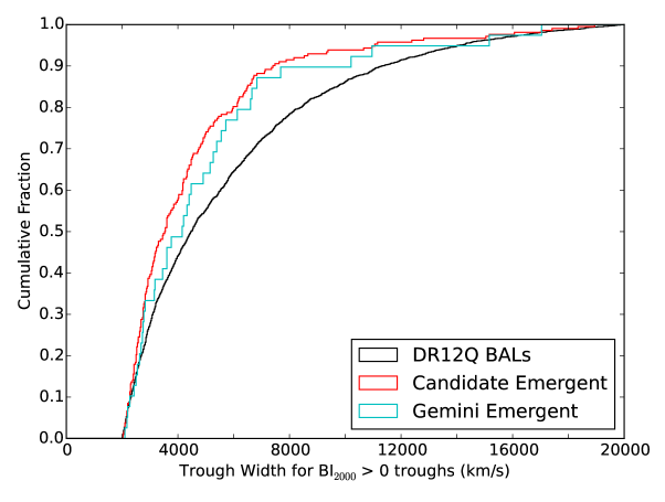
Figure 17: The cumulative distribution functions (CDFs) of average DR12Q BAL trough widths in non-emergent DR12Q BAL quasars (black), candidate emergent DR12Q BAL quasars (red), and emergent DR12Q BAL quasars with Gemini spectra (cyan).

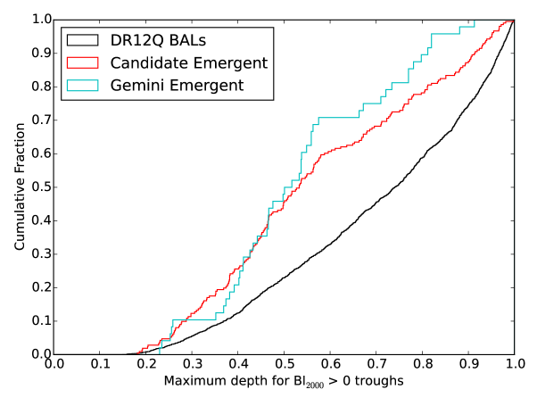
Figure 18: The cumulative distribution functions (CDFs) of DR12Q BAL trough depths in non-emergent DR12Q BAL quasars (black), candidate emergent DR12Q BAL quasars (red), and emergent DR12Q BAL quasars with Gemini spectra (cyan).

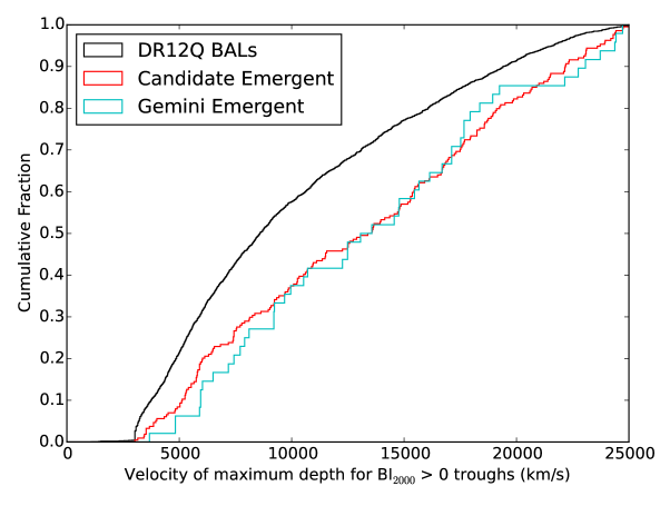
Figure 19: The cumulative distribution functions (CDFs) of the velocities of DR12Q BAL trough maximum depths in non-emergent DR12Q BAL quasars (black), candidate emergent DR12Q BAL quasars (red), and emergent DR12Q BAL quasars with Gemini spectra (cyan).

4.6 What Happens to the Absorption After it Emerges?

Our original candidate sample was targeted for visual identification of emergent absorption. Thus our sample is biased toward an increase in EW when comparing an SDSS observation to a BOSS observation. In Figure 20, the change in EW ($\Delta$EW) measured between SDSS and BOSS observations is compared to the change in the same absorption complex between the BOSS observation and our Gemini observation. Note that there are some quasars with multiple SDSS and/or BOSS observations, but the figure only plots the two with the shortest separation in time (i.e., SDSS2-BOSS1); in target selection, these were the spectra that were visually compared. Thus, for each absorption complex, we have one point for the figure. There are 3 exceptions: the quasars that were not discovered until SDSS Data Release 9 (see § 2.5); they are not included in the plot.

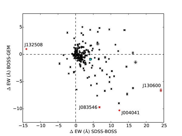
Figure 20: Comparing the change in EW between the SDSS and BOSS observations to the same quasar’s change in EW between the BOSS and GEM observations. The 4 red points are the extreme cases shown in Fig. 21. The cyan square is the weighted-mean value of all the points in the plot.

Most of the data points are found to the right of $\Delta\textrm{EW SDSS-BOSS}=0$, indicating an absorption feature’s EW usually but not always increased between SDSS and BOSS observations. This result is expected because in building the visually identified emergent sample in § 2.1, we only searched for new troughs, not new BAL quasars; thus, we expect a small number of weakening pre-existing troughs in a sample with most objects having increasing EW. Further, $\sim$ 60% of the data points are below $\Delta\textrm{EW BOSS-GEM}=0$, indicating the EW of an absorption feature usually got smaller between the BOSS and Gemini observations. The cyan point shows the weighted-mean values of $\Delta$EW of $4.16\pm 0.10$ Å from SDSS to BOSS and $-0.93\pm 0.09$ Å from BOSS to Gemini. The four red points in Figure 20 are highlighted because they exhibit extreme changes in EW between both SDSS to BOSS observations and BOSS to Gemini observations. Their spectra are plotted in Figure 21. J132508 exhibited a large decrease in EW from SDSS to BOSS observations. The spectra indicate that a strong absorber at small velocities completely disappeared between the two observations. J132508 was originally targeted for a possible absorber emerging at $v>40,000$ km s^-1, but the larger wavelength coverage of the Gemini observation showed that candidate absorber to be spurious. J130600 exhibits some of the strongest absorption seen in our entire dataset, and the strongest increase in EW from SDSS to BOSS. In the BOSS spectrum of J083546 there is strengthening of the C iv absorption on top of its Si iv emission, but the absorption was weaker in the first Gemini epoch (cyan) than in the original SDSS epoch. Finally, J004041 exhibited a large, albeit shallow, increase in C iv absorption between SDSS2 (grey) to BOSS (blue); this increase was almost completed reversed in the Gemini epoch (cyan).

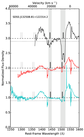
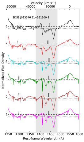
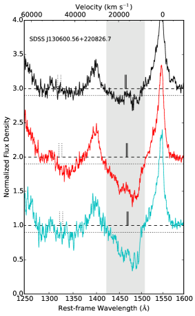
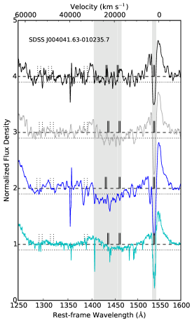
Figure 21: The four quasars highlighted as red points in Fig. 20 represent some of the most extreme changes in absorption measured in this dataset. Each quasar’s spectra are plotted, with the oldest spectrum is at the top with each successive spectrum in chronological order below it. Colors represent the differing observational origins of each spectrum. See Appendix LABEL:app:figures for more information on these figures.

4.6.1 Conditional probabilities of absorption changes

We now consider in more detail how a previous change in equivalent width could predict the change in EW between the next two epochs. We are interested in how troughs behave after a change has been observed. If a trough changes its EW, what is it most likely to do next? Will it continue to change in the same way? Or will it reverse its change? And on what time-scales? Our goal is to determine how well a history of increases (or decreases) in absorption could predict what the absorption would do next.

We utilize our full suite of 3-7 epochs for each quasar. For a given quasar, we first compare the EWs between the first and second observations. The EW change can either be an increase, a decrease, or within the uncertainties (i.e., no statistically significant change). Next we compare the change in EW between the second and third observations and determine if it was an increase, a decrease, or within the uncertainties. If both changes in EW were increases or both changes in EW were decreases, we label the EW trend ‘staying the same’. If the first change in EW is an increase but the second is a decrease (or vice versa), we label the EW trend ‘changed’. If the EW changes are within the uncertainties we label the EW trend ‘uncertain’.

There were, however, some caveats to the above prescription. Below is an itemized list of how we built this analysis, assuming a quasar has been observed $n$ times (i.e., epoch₁ $\cdots$ epoch_n).

1. Determine the reference point. The reference point is the first change of EW from one epoch to another that is significant at $\geq 3\sigma_{EW}$. Start with the first observation, epoch₁, and search for a reference point in this order: epoch₁-epoch₂, epoch₂-epoch₃, epoch₁-epoch₃, epoch₃-epoch₄.

2. If epoch₁-epoch₂ is SDSS1-SDSS2, ignore it unless epoch₂-epoch₃ showed no statistically significant change in EW. As our visual sample was built around searching for emergence between SDSS-BOSS, we set that to be the reference point as much as possible.

3. Determine the sign of the change in EW from the reference point, either positive for increasing absorption or negative for decreasing absorption.

4. Compare the reference point to the next epoch change. For example, if the reference point was epoch_n-epoch_n+1, determine whether the change in EW over epoch_n+1-epoch_n+2 is in the same direction or opposite to the reference point. Record the $\Delta T$ between epoch_n+1-epoch_n+2. However, if no statistically significant change in EW occurred between epoch_n+1-epoch_n+2, then compare the reference point to epoch_n+1-epoch_n+3, epoch_n+1-epoch_n+m, etc., until a significant change is found.

5. Reset the reference point to epoch_n+1-epoch_n+m, the first two epochs between which a statistically significant change in EW was found to occur.

6. Return to step 3 and repeat until there are no more epochs.

The result of the above analysis is plotted in Figure 22. The plot incorporates three histograms, each with five bins in $\Delta T$, with the total of all three histograms summing to unity in each bin. The $\Delta$T on the x-axis is the time frame between the second and third epochs in the analysis (see Step 4). The histogram widths were chosen to place 50 measurements in each bin (in an effort standardize the number statistics for each bin). The cyan histogram shows the number of troughs that continued to increase in EW after an increase was already observed (’same’). The red histogram shows the number of troughs that switched their direction of variability (’changed’). The grey histogram shows the cases where the direction of variability was unclear (’uncertain’).

Within the uncertainties, we are unable to tell the difference between the red and cyan histograms. On the time-scales between our 2nd and 3rd epochs, quasars are equally likely to continue increasing/decreasing or to stay the same. Thus, the time-scale between two observations such that the first observation can predict the second observation (the coherence time-scale) must be less than 150 days, based on bin-size in Figure 22. This result is consistent with the results found by Grier et al. (2015), using spectroscopic monitoring of one BAL quasar on timescales $<$150 days, and by Gibson et al. (2010), who found that BAL variability on month-long timescales was not predictive of BAL variability on multi-year timescales. Our results are also consistent with the random-walk model for the evolution of BAL troughs presented in §5.4 of Filiz Ak et al. (2013), in which BAL trough EW variability is modeled as occurring in uncorrelated steps every $140\pm 50$ days, on average.

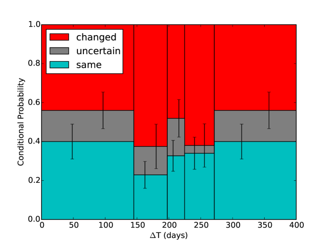
Figure 22: Conditional probability of absorption trend between the 2nd and 3rd epochs continuing in the same direction as observed between the 1st and 2nd epochs, as a function of $\Delta T$ between the 2nd and 3rd epochs. See text of § 4.6.1 for details.

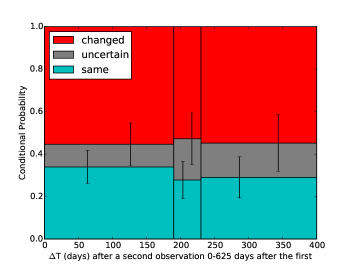
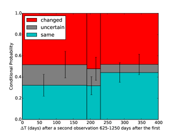
Figure 23: Same as Figure 22, except split into one panel for observations where the $\Delta T$ between the 1st and 2nd epochs was less than 650 days and one panel where it was greater than 650 days. There is no significant difference between the two cases.

These results remain unchanged if we distinguish between observations with smaller and larger values of $\Delta T$ between the first two spectroscopic epochs. To make that comparison, we make separate conditional probability histograms for observations with $\Delta T<625$ days and with $625<\Delta T<1250$ days, using only three bins in $\Delta T$ between the second and third spectroscopic epochs for each histogram. The results are shown in Figure 23. No significant difference is seen between those histograms and that shown in Figure 22.

In each absorption complex in each quasar, the EW trend over three epochs can vary in one of three ways: it can stay the same direction (whether increasing or decreasing), change direction, or be uncertain. We have examined the frequency with which all complexes in the same quasar behave the same way in our observations. In 15 objects (5 with more than one complex) the EW trend in all complexes present stays the same, in 31 objects (15 with more than one complex) the EW trend in all complexes present changes direction, and in 8 objects (2 with more than one complex) all complexes present show uncertain changes. The remaining objects have complexes that do not all change in the same way; about two-thirds of all objects with more than one complex fall into this category. Targets observed with sufficiently short time differences between epochs (and at sufficiently high SNR) are in principle be more likely to show EW trends that stay the same. The time differences between epochs in our study are not short enough for that effect to be seen: K-S tests reveal no statistical difference between any of the above subsamples’ $\Delta t_{12}$, $\Delta t_{23}$, or $\Delta t_{13}$ distributions.

4.7 Coordinated Variability

Many of the quasars in our dataset have more than one trough of the same species varying in their spectra. Comparing how the troughs vary with respect to one another can help distinguish models of outflows. For example, if two troughs from the same species in the same quasar both increase their EW at the same time, or decrease their EW at the same time, it indicates the source of the variability is affecting different outflowing absorbers similarly. This is called coordinated variability. Two troughs could also vary opposite to each other: when one increases in EW, the other decreases. This is called anticoordinated variability.

It would be difficult to explain coordinated variability in the context of the transverse motion of clouds across the line of sight to the quasar. A more natural explanation is the total ionizing flux incident upon the various individual troughs (from the central source) has increased or decreased and is thereby responsible for global changes in the absorption, regardless of outflow velocity of the trough. Thus the most likely cause of coordinated variability in BAL troughs would be a result of changes in the ionizing flux incident upon the absorber. Coordinated variability has been observed and interpreted previously in e.g., Filiz Ak et al. (2012), Filiz Ak et al. (2013), and Wang et al. (2015).

To determine whether coordinated variability was occurring in our dataset, we took all quasars with more than one absorption complex and calculated the change in EW between successive epochs for each complex. A complex was considered to be increasing/decreasing in absorption if the change in EW was larger than 3 times the statistical noise propagated from the EW uncertainties. We then compared each complex’s direction of change of EW to that of each other absorption complex in the quasar.

Table 6 gives the conditional probabilities of how a complex changed given the condition set by another complex in the quasar. From the table, if an absorption complex EW was measured to be increasing, then each other absorption complex EW in that quasar has a 69.8 % chance of increasing over the same time frame (300 out of the 430 such cases). If an absorption complex EW was measured to be decreasing, each other absorption complex EW in that quasar has a 65.9 % chance to also be decreasing (182 out of 276 such cases). Both of these situations are considered coordinated variability. Overall, if a statistically significant change is seen in one complex in a quasar, there is a $(300+182)/(276+430)=68.3$ % rate of coordinated variability in other complexes in the same quasar. The rate of anticoordinated variability is $(70+70)/(430+276)=19.8$ %. Only in 11.9 % of cases does a complex not vary statistically significantly when another complex in the quasar does. We outlined in § 4.7 of Filiz Ak et al. (2013) how to derive the minimum fraction of observed variability arising from a mechanism that produces coordinated variability. Random chance will produce an equal mixture of coordinated and anticoordinated variability, so that some apparently coordinated variations will be due to chance. To correct for that effect, we can take the rate of anticoordinated variability and subtract it from the rate of coordinated variability to estimate the fraction of BAL EW variability arising from a coordinated process. The result is that a minimum of 48.5 % $\pm$ 3.5 % of BAL variability must be due to a mechanism that produces coordinated variability (see also He et al. 2017).

With such a strong signal of coordinated variability, we investigated whether velocity separation between absorption complexes had an impact on the conditional probabilities of the other complexes. In Figure 24, the cumulative distribution functions (CDFs) of coordinated variability (black) versus anticoordinated variability (red) are plotted as a function of difference in centroid velocity. Also plotted is the distribution of cases where no statistically significant change (within the uncertainties) occurred from one observation to the next in a given complex; this is labeled unknown and plotted in cyan. Applying the two-sample Kuiper test to the coordinated/anticoordinated distributions results in a probability of 1.7 % that the two distributions are the same. Thus, the distributions of velocities for coordinated and anticoordinated variability are statistically different at 98.3 % probability. This again suggests there must be two different mechanisms producing coordinated and anticoordinated variability.

The incidence of anticoordinated variability increases at larger velocity separations. In other words, the farther apart troughs are in velocity space, the less likely they are to have coordinated variability.

Applying the Kuiper test to compare the coordinated and unknown CDFs results in a probability of $\sim 10^{-4}$ that the two histograms are drawn from the same distribution. The coordinated histogram is different from the unknown histogram at high significance. Finally, the Kuiper test comparing the anticoordination versus the CDF results in a probability the two distributions are the same of 15 %. We cannot reject the hypothesis that the anticoordination and the unknown CDFs are drawn from the same sample.

Table 6: The conditional probability, given a change in EW for one absorption complex in a quasar, for what other complexes in the same quasar were doing. The first column indicates the condition set by some complex, and the following columns indicate the probabilities of other complexes in a quasar varying in specific ways. ‘Increase’ is a complex which increased in EW between two observations, ‘same’ is a complex which has not changed within the statistical uncertainties, and ‘decrease’ is a complex which has decreased in EW between two observations.

condition	increase	same	decrease	total
increase	69.8% (300)	13.9% (60)	16.3% (70)	430
same	60% (60)	16% (16)	24% (24)	100
decrease	25.4% (70)	8.69% (24)	65.9% (182)	276

It is clear there is coordinated variability happening in the dataset. To investigate whether the relative locations in velocity space of coordinated/anticoordinated complexes matter, we performed a more detailed analysis. Absorption complexes were only compared to other complexes at higher velocities, and we retained the information on velocity separation, $\Delta$T between observations, and the direction (increasing or decreasing) of the variability. We followed these steps for each quasar:

1. For a given quasar, collect all absorption information for each complex for all spectra available, except that we removed comparisons between SDSS1 and SDSS2 observations due to the higher noise levels in both epochs making $\Delta EW$ measurements very uncertain.

2. Sort the complexes in ascending velocity order (i.e., closest to C iv emission to furthest).

3. Compare first complex to second, third, …, $n$th. For each comparison record direction of coordination (see below), separation in centroid velocity, and $\Delta$T between observations.

4. Compare second complex to third, …, $n$th. For each comparison record direction of coordination (see below), separation in centroid velocity, and $\Delta$T between observations.

5. Repeat until no more absorption complexes to compare in the quasar.

The results of this analysis are given in Table 7. The numbers of cases considered is one-half of those considered in the previous table because in the above analysis we compared complexes to others at both lower and higher velocities.

As was argued above, if we assume that all comparisons between two troughs will give a mixture of both coordinated and anticoordinated variability, and thus remove the effect of anticoordinated variability (19.3 %) from the rate of coordinated variability (66.6 %), there is at minimum a 47.3 % rate of coordinated variability motivated by some underlying mechanism and not by chance.

In Figure 25 are the cumulative distribution functions for the data in Table 7. In the Figure, we have separated out the differing possibilities for how troughs can respond with respect to one another. The symbol ‘$++$’ indicates the case when two troughs have increased in absorption at the same time, while ‘$--$’ indicates both decreased. The two anticoordination cases are ‘$-+$’ and ‘$+-$’; the former is when the lower-velocity absorption complex is decreasing in EW while the higher-velocity absorption complex is increasing, and the latter is when the higher-velocity absorption complex is decreasing while the lower-velocity absorption complex is increasing in EW. All cases in which no statistically significant change was measured in either or both troughs are labeled ‘$0$’.

It is clear that both cases of coordinated variability are similar to each other; the Kuiper test yields a 42 % probability that both CDFs are drawn from the same sample, meaning there is no favoured direction of coordinated variability. While in the figure there is an obvious difference between the ‘$-+$’ and ‘$+-$’ cases of anticoordinated variability, the Kuiper test between these two cases indicates a probability of 56 % that those two CDFs are actually drawn from the same sample. Small-number statistics mean that the apparent difference between the ‘$+-$’ and ‘$-+$’ histograms, while intriguing, cannot be interpreted as real until better statistics are obtained.

Both Figure 24 and 25 show that coordinated variability is happening, and the troughs closer together in velocity are more likely to vary in a coordinated way. We speculate that this result arises from density considerations. Higher velocity outflows are likely to have lower densities due to mass conservation in an accelerating flow. Since the ionization response time of an absorbing cloud is related to its density, it is plausible that two outflows in the same quasar with a large separation in velocity would be less likely to vary in unison. The density in an accelerating flow with velocity $v(r)$ satisfies the continuity equation $n(r)A(r)v(r)={\rm constant}$, where $A(r)$ is the cross-sectional area of the flow as a function of distance $r$ from the launch point. If $A(r)$ is constant, then $n\propto 1/v$. For example, Figure 4 of Murray et al. (1995) shows that $n$ drops by a factor of $10^{3}$ as the velocity increases by a factor of $10^{3}$ beyond the sonic point of a disk wind outflow, and then $n$ drops further as the gas coasts to larger radii at its terminal velocity (constant $v$ but increasing $A$). The timescale needed for gas to respond to ionizing flux changes can often be approximated as $t\propto 1/n\alpha$ where $\alpha$ is the relevant recombination coefficient Grier et al. (2015). Thus, in clumps expanding in an accelerating flow, gas at two different outflow velocities will have a ratio of response timescales $t_{hi}/t_{lo}>v_{hi}/v_{lo}$ for $v_{lo}>10$ km s^-1 (an estimate of the turbulent sound speed). Our sample of absorbers at 1000 to 60,000 km s^-1 could span a factor of $>60$ range in response timescales, and even a factor of 10 is sufficient to show anticoordination in response to the same underlying ionizing flux (Figure 4 of Arav et al. 2012).

Table 7: The conditional probability, given a change in EW for one absorption complex in a quasar, for what other complexes at higher velocities in the same quasar were doing. The format is the same as for Table 6.

condition	increase	same	decrease	total
increase	69.4% (150)	18.1% (39)	12.5% (27)	216
same	51.2% (21)	19.5% (8)	29.3% (12)	41
decrease	29.4% (43)	8.2% (12)	62.3% (91)	146

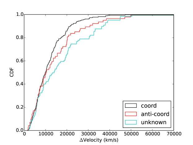
Figure 24: The cumulative distribution functions (CDFs) of coordinated variability (black) versus anticoordinated variability (red). For these CDFs, each absorption complex from a given quasar was compared to every other complex, which results in double counting.

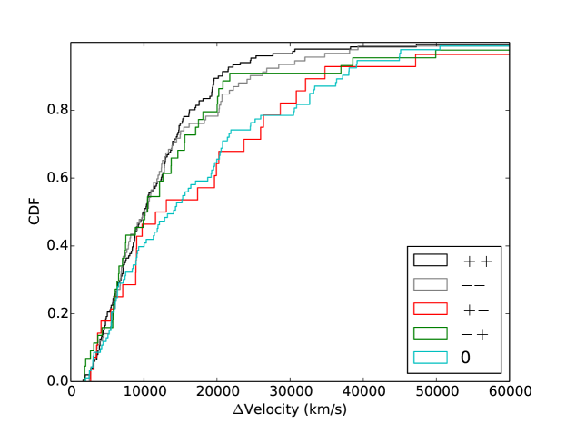
Figure 25: This plot removes double counting and separates out the different cases of coordination/anticoordination. Cases are indicated by: ‘$++$’ when two troughs increased in EW together, ‘$--$’ when two troughs decreased in EW together, ‘$-+$’ when the lowest-velocity trough decrease in EW while the other increased, ‘$+-$’ when the lowest-velocity trough increased in EW while the other decreased, and finally ‘0’ for all cases that involved a change that was below the 3$\sigma$ statistical noise limit.

5 Conclusions

Below is a summary of the notable conclusions found in this work.

1. Visual comparison of multiple spectra of the same quasar from SDSS DR7 and DR9 or DR7 and DR10 yielded 306 visually identified candidates for newly emerged BAL troughs. Absorption was quantitatively confirmed in 103 out of the 105 of these cases which were followed up with Gemini spectroscopy. Thus, the visual inspection is robust. See § 2.1.

2. Using a modified version of the BALnicity Index, 653 individual broad absorption troughs were identified in 360 spectra of the 105 targets in our dataset. Each trough was at least 1,000 km s^-1 wide and found anywhere between $0<v~{}(\textrm{km~{}s${}^{-1}$})<$ 65,000, where 0 km s^-1 is at the systemic redshift of the quasar, and positive velocities are toward the observer. See § 2.8.

3. To account for troughs splitting apart or merging into one between epochs, we defined an absorption complex to be a region in a quasar spectrum that, over the multiple spectra available, has had one or more BAL trough in at least one epoch. The 653 individual troughs are reduced to 219 absorption complexes by this definition. See § 3.1.

4. In the sample of 105 quasars, there were 36 instances of a quasar transitioning from non-BAL to BAL. By design, this mostly occurred in the SDSS-BOSS transition. There were 11 cases of quasars transitioning from BAL to non-BAL. See § 4.2.

5. The visually identified BAL trough emergence rate at $z>1.68$ in our sample was $1.87\pm 0.11$ % over rest-frame timescales of $1-3$ years. The rate of emergence of BAL quasars from objects previously classified as non-BAL quasars was $0.59\pm 0.12$ %. We find that our BAL quasar emergence rates and the BAL quasar disappearance rates of (Filiz Ak et al., 2012) are in agreement for a BAL quasar fraction in the parent sample of $f_{BAL}=0.26^{+0.09}_{-0.12}$. See § 4.3.

6. We find that candidate newly emerged BAL quasar troughs are preferentially drawn from among BAL troughs with smaller balnicity indices, shallower depths, larger velocities, and smaller widths. See § 4.5.

7. As expected, the weighted-mean change in absorption equivalent width $\Delta$EW from SDSS to BOSS was $4.16\pm 0.10$ Å, an increase in EW. After the SDSS-BOSS transition, however, there was a significant trend for the EW to decrease. The weighted-mean $\Delta$EW from BOSS-GEM was $-0.93\pm 0.09$ Å. See § 4.6.

8. Despite the above averages, a more detailed analysis that took into account the time between observations found: if an absorption complex begins to increase in EW between two observations, it is equally likely to continue increasing in the next observation, as it is to switch to decreasing. Based on our analysis this indicates the coherence time-scale of BAL EW variations must be less than 150 days. See § 4.6.

9. Coordinated variability, when two absorption complexes in the same quasar increase or decrease in EW at the same time, occurs at a rate of 68.3 %. Anticoordinated variability occurs at a rate of 19.8 %. This likely indicates that ionizing flux variations contribute to at least 48.5 % $\pm$ 3.5 % of all BAL EW variability. See § 4.7.

10. Troughs that are closer together in velocity space are more likely to exhibit coordinated variability than those further apart in velocity space, at 98.3 % significance. This dependence of coordinated variability on velocity separation may be related to cloud densities. If clouds decrease in density as they accelerate, higher-velocity clouds would respond to changes in the ionizing flux differently than lower-velocity clouds. There is also a suggestion of different velocity distributions for cases of a lower velocity trough increasing in EW while a higher velocity trough decreases in EW as compared to the reverse; however, small number statistics prevent a determination of whether the suggested difference is statistically significant or not. See § 4.7.

11. The change in equivalent width, $\Delta$EW, with respect to time between successive observations in our data merges smoothly with the distribution seen in the literature. Our data filled in the region on rest-frame time-scales of $0.5-1.0$ years that been largely unexplored in the literature. See Figure 14.

5.1 Future Directions

In § 4.6, we attempted to determine if a BAL’s past variability was a predictor of its variability in the future. Unfortunately, our dataset did not have the number statistics, nor the time resolution to conclude that it could. Certainly one can imagine that if a trough were to be observed from zero EW to a full trough with multiple spectral epochs, it would be possible to use a history of increasing strength of absorption to predict the trough will continue to increase with some constraint on time. In our dataset, that coherence time-scale must be less than 100 days in the rest-frame. Performing a monitoring program with high time resolution for a medium-sized set of quasars would help determine a coherence scale. For example, a set of 10 bright BAL quasars observed once a week for an entire observing semester would provide enough data to answer this question. It would be recommended to choose a set of quasars from the dataset presented herein, due to the already confirmed variable absorption in them.

A monitoring program focused on high time resolution could inform understanding on the nature of coordinated variability as well. We observed an apparent difference between two types of anticoordinated variability that would challenge our understanding of the quasar model if it were proven correct. The only way to determine its validity would be a campaign of observations on quasars with multiple troughs with higher time resolution.

In the dataset presented here, a few quasars presented very complicated and informative variability. Our separately published case study of J023011 (Rogerson et al., 2016) is an example of how targeted studies can lead to more specific results. In that study, we showed how the observed short-timescale absorption variability in J023011 could be used to constrain one of the absorber’s physical parameters, depending on the cause of EW variability: its electron density in the case of ionization balance changes, or its transverse velocity in the case of bulk motion of gas across the line of sight. To that end, continued monitoring of quasar J015017 (see Figure 13) could help disentangle the different signals of ionization changes and bulk motion.

References

- Abazajian et al. (2009) Abazajian, K. N., Adelman-McCarthy, J. K., Agüeros, M. A., et al. 2009, ApJS, 182, 543
- Ahn et al. (2012) Ahn, C. P., Alexandroff, R., Allende Prieto, C., et al. 2012, ApJS, 203, 21
- Ahn et al. (2014) —. 2014, ApJS, 211, 17
- Allen et al. (2011) Allen, J. T., Hewett, P. C., Maddox, N., Richards, G. T., & Belokurov, V. 2011, MNRAS, 410, 860
- Arav et al. (2013) Arav, N., Borguet, B., Chamberlain, C., Edmonds, D., & Danforth, C. 2013, MNRAS, 436, 3286
- Arav et al. (2012) Arav, N., Edmonds, D., Borguet, B., et al. 2012, A&A, 544, A33
- Barlow (1994) Barlow, T. A. 1994, PASP, 106, 548
- Capellupo et al. (2011) Capellupo, D. M., Hamann, F., Shields, J. C., Rodríguez Hidalgo, P., & Barlow, T. A. 2011, MNRAS, 413, 908
- Chamberlain et al. (2015) Chamberlain, C., Arav, N., & Benn, C. 2015, MNRAS, 450, 1085
- Dawson et al. (2013) Dawson, K. S., Schlegel, D. J., Ahn, C. P., et al. 2013, AJ, 145, 10
- Eisenstein et al. (2011) Eisenstein, D. J., Weinberg, D. H., Agol, E., et al. 2011, AJ, 142, 72
- Elvis (2000) Elvis, M. 2000, ApJ, 545, 63
- Filiz Ak et al. (2012) Filiz Ak, N., Brandt, W. N., Hall, P. B., et al. 2012, ApJ, 757, 114
- Filiz Ak et al. (2013) —. 2013, ApJ, 777, 168
- Foltz et al. (1986) Foltz, C. B., Weymann, R. J., Peterson, B. M., et al. 1986, ApJ, 307, 504
- Ganguly & Brotherton (2008) Ganguly, R., & Brotherton, M. S. 2008, ApJ, 672, 102
- Gibson et al. (2010) Gibson, R. R., Brandt, W. N., Gallagher, S. C., Hewett, P. C., & Schneider, D. P. 2010, ApJ, 713, 220
- Gibson et al. (2008) Gibson, R. R., Brandt, W. N., Schneider, D. P., & Gallagher, S. C. 2008, ApJ, 675, 985
- Grier et al. (2015) Grier, C. J., Hall, P. B., Brandt, W. N., et al. 2015, ApJ, 806, 111
- Gunn et al. (1998) Gunn, J. E., Carr, M., Rockosi, C., et al. 1998, AJ, 116, 3040
- Gunn et al. (2006) Gunn, J. E., Siegmund, W. A., Mannery, E. J., et al. 2006, AJ, 131, 2332
- Haggard et al. (2012) Haggard, D., Arraki, K. S., Green, P. J., Aldcroft, T., & Anderson, S. F. 2012, in Astronomical Society of the Pacific Conference Series, Vol. 460, AGN Winds in Charleston, ed. G. Chartas, F. Hamann, & K. M. Leighly, 98
- Hall et al. (2011) Hall, P. B., Anosov, K., White, R. L., et al. 2011, MNRAS, 411, 2653
- Hall et al. (2002) Hall, P. B., Anderson, S. F., Strauss, M. A., et al. 2002, ApJS, 141, 267
- Hall et al. (2013) Hall, P. B., Brandt, W. N., Petitjean, P., et al. 2013, MNRAS, 434, 222
- Hamann et al. (2008) Hamann, F., Kaplan, K. F., Rodríguez Hidalgo, P., Prochaska, J. X., & Herbert-Fort, S. 2008, MNRAS, 391, L39
- He et al. (2015) He, Z.-C., Bian, W.-H., Ge, X., & Jiang, X.-L. 2015, MNRAS, 454, 3962
- Kaspi et al. (2002) Kaspi, S., Brandt, W. N., George, I. M., et al. 2002, ApJ, 574, 643
- Krongold et al. (2010) Krongold, Y., Binette, L., & Hernández-Ibarra, F. 2010, ApJ, 724, L203
- Landolt (1992) Landolt, A. U. 1992, AJ, 104, 340
- Leighly et al. (2009) Leighly, K. M., Hamann, F., Casebeer, D. A., & Grupe, D. 2009, ApJ, 701, 176
- Leighly et al. (2014) Leighly, K. M., Terndrup, D. M., Baron, E., et al. 2014, ApJ, 788, 123
- Lundgren et al. (2007) Lundgren, B. F., Wilhite, B. C., Brunner, R. J., et al. 2007, ApJ, 656, 73
- Lynds (1967) Lynds, C. R. 1967, ApJ, 147, 396
- McGraw et al. (2017) McGraw, S. M., Brandt, W. N., Grier, C. J., et al. 2017, ArXiv e-prints, arXiv:1705.03019
- Moe et al. (2009) Moe, M., Arav, N., Bautista, M. A., & Korista, K. T. 2009, ApJ, 706, 525
- Morton (1991) Morton, D. C. 1991, ApJS, 77, 119
- Murray et al. (1995) Murray, N., Chiang, J., Grossman, S. A., & Voit, G. M. 1995, ApJ, 451, 498
- Ostriker et al. (2010) Ostriker, J. P., Choi, E., Ciotti, L., Novak, G. S., & Proga, D. 2010, ApJ, 722, 642
- Pâris et al. (2012) Pâris, I., Petitjean, P., Aubourg, É., et al. 2012, A&A, 548, A66
- Pâris et al. (2014) —. 2014, A&A, 563, A54
- Pâris et al. (2017) Pâris, I., Petitjean, P., Ross, N. P., et al. 2017, A&A, 597, A79
- Press et al. (2007) Press, W. H., Teukolsky, S. A., Vetterling, W. T., & Flannery, B. P. 2007, Numerical Recipes, 3rd Edition (Cambridge: Cambridge University Press), 731
- Proga & Kallman (2004) Proga, D., & Kallman, T. R. 2004, ApJ, 616, 688
- Proga et al. (2012) Proga, D., Rodriguez-Hidalgo, P., & Hamann, F. 2012, in Astronomical Society of the Pacific Conference Series, Vol. 460, AGN Winds in Charleston, ed. G. Chartas, F. Hamann, & K. M. Leighly, 171
- Rodríguez Hidalgo et al. (2013) Rodríguez Hidalgo, P., Eracleous, M., Charlton, J., et al. 2013, ApJ, 775, 14
- Rodríguez Hidalgo et al. (2011) Rodríguez Hidalgo, P., Hamann, F., & Hall, P. 2011, MNRAS, 411, 247
- Rogerson et al. (2012) Rogerson, J. A., Hall, P. B., MacLeod, C., & Ivezić, Ž. 2012, in Astronomical Society of the Pacific Conference Series, Vol. 460, AGN Winds in Charleston, ed. G. Chartas, F. Hamann, & K. M. Leighly, 124
- Rogerson et al. (2016) Rogerson, J. A., Hall, P. B., Rodríguez Hidalgo, P., et al. 2016, MNRAS, 457, 405
- Savitzky & Golay (1964) Savitzky, A., & Golay, M. J. E. 1964, Analytical Chemistry, 36, 1627
- Schneider et al. (2010) Schneider, D. P., Richards, G. T., Hall, P. B., et al. 2010, AJ, 139, 2360
- Smee et al. (2013) Smee, S. A., Gunn, J. E., Uomoto, A., et al. 2013, AJ, 146, 32
- Trump et al. (2006) Trump, J. R., Hall, P. B., Reichard, T. A., et al. 2006, ApJS, 165, 1
- Vanden Berk et al. (2001) Vanden Berk, D. E., Richards, G. T., Bauer, A., et al. 2001, AJ, 122, 549
- Wang et al. (2015) Wang, T., Yang, C., Wang, H., & Ferland, G. 2015, ApJ, 814, 150
- Weymann et al. (1991) Weymann, R. J., Morris, S. L., Foltz, C. B., & Hewett, P. C. 1991, ApJ, 373, 23
- York et al. (2000) York, D. G., Adelman, J., Anderson, J. E., et al. 2000, AJ, 120, 1579