Spectral characterizations of anti-regular graphs

Abstract.

We study the eigenvalues of the unique connected anti-regular graph $A_{n}$. Using Chebyshev polynomials of the second kind, we obtain a trigonometric equation whose roots are the eigenvalues and perform elementary analysis to obtain an almost complete characterization of the eigenvalues. In particular, we show that the interval $\Omega=[\tfrac{-1-\sqrt{2}}{2},\tfrac{-1+\sqrt{2}}{2}]$ contains only the trivial eigenvalues $\lambda=-1$ or $\lambda=0$, and any closed interval strictly larger than $\Omega$ will contain eigenvalues of $A_{n}$ for all $n$ sufficiently large. We also obtain bounds for the maximum and minimum eigenvalues, and for all other eigenvalues we obtain interval bounds that improve as $n$ increases. Moreover, our approach reveals a more complete picture of the bipartite character of the eigenvalues of $A_{n}$, namely, as $n$ increases the eigenvalues are (approximately) symmetric about the number $-\tfrac{1}{2}$. We also obtain an asymptotic distribution of the eigenvalues as $n\rightarrow\infty$. Finally, the relationship between the eigenvalues of $A_{n}$ and the eigenvalues of a general threshold graph is discussed.

1. Introduction

Let $G=(V,E)$ be an $n$-vertex simple graph, that is, a graph without loops or multiple edges, and let $\deg_{G}(v)$ denote the degree of $v\in V$. It is an elementary exercise to show that $G$ contains at least two vertices of equal degree. If $G$ has all vertices with equal degree then $G$ is called a regular graph. We say then that $G$ is an anti-regular graph if $G$ has only two vertices of equal degree. If $G$ is anti-regular it follows easily that the complement graph $\overline{G}$ is also anti-regular since $\deg_{G}(v)=(n-1)-\deg_{\overline{G}}(v)$. It was shown in [2] that up to isomorphism, there is only one connected anti-regular graph on $n$ vertices and that its complement is the unique disconnected $n$-vertex anti-regular graph. Let us denote by $A_{n}$ the unique connected anti-regular graph on $n\geq 2$ vertices. The graph $A_{n}$ has several interesting properties. For instance, it was shown in [3] that $A_{n}$ is universal for trees, that is, every tree graph on $n$ vertices is isomorphic to a subgraph of $A_{n}$. Anti-regular graphs are threshold graphs [4] which have numerous applications in computer science and psychology. Within the family of threshold graphs, the anti-regular graph is uniquely defined by its independence polynomial [7]. Also, the eigenvalues of the Laplacian matrix of $A_{n}$ are all distinct integers and the missing eigenvalue from $\{0,1,\ldots,n\}$ is $\lfloor(n+1)/2\rfloor$. In [6], the characteristic and matching polynomial of $A_{n}$ are studied and several recurrence relations are obtained for these polynomials, along with some spectral properties of the adjacency matrix of $A_{n}$.

In this paper, we study the eigenvalues of the adjacency matrix of $A_{n}$. If $V(G)=\{v_{1},\ldots,v_{n}\}$ is the vertex set of the graph $G$ then the adjacency matrix of $G$ is the $n\times n$ symmetric matrix $A$ with entry $A(i,j)=1$ if $v_{i}$ and $v_{j}$ are adjacent and $A(i,j)=0$ otherwise. From now on, whenever we refer to the eigenvalues of a graph we mean the eigenvalues of its adjacency matrix. It is known that the eigenvalues of $A_{n}$ have algebraic multiplicity equal to one and take on a bipartite character [6] in the sense that if $n$ is even then half of the eigenvalues are negative and the other half are positive, and if $n$ is odd then $\lambda=0$ is an eigenvalue and half of the remaining eigenvalues are positive and the other half are negative. Our approach to studying the eigenvalues of $A_{n}$ relies on a natural labeling of the vertices that results in a block triangular structure for the inverse adjacency matrix. The blocks are tridiagonal pseudo-Toeplitz matrices and Hankel matrices. We are then able to employ the connection between tridiagonal Toeplitz matrices and Chebyshev polynomials to obtain a trigonometric equation whose roots are the eigenvalues. Performing elementary analysis on the roots of the equation we obtain an almost complete characterization of the eigenvalues of $A_{n}$. In particular, we show that the only eigenvalues contained in the closed interval $\Omega=[\tfrac{-1-\sqrt{2}}{2},\tfrac{-1+\sqrt{2}}{2}]$ are the trivial eigenvalues $\lambda=-1$ or $\lambda=0$, and any closed bounded interval strictly larger than $\Omega$ will contain eigenvalues of $A_{n}$ for all $n$ sufficiently large. This improves a result in [10] obtained for general threshold graphs and we conjecture that $\Omega$ is a forbidden eigenvalue interval for all threshold graphs (besides the trivial eigenvalues $\lambda=0$ or $\lambda=-1$). We also obtain bounds for the maximum and minimum eigenvalues, and for all other eigenvalues we obtain interval bounds that improve as $n$ increases. Moreover, our approach reveals a more complete picture of the bipartite character of the eigenvalues of $A_{n}$, namely, as $n$ increases the non-trivial eigenvalues are (approximately) symmetric about the number $-\tfrac{1}{2}$. Lastly, we obtain an asymptotic distribution of the eigenvalues as $n\rightarrow\infty$. We conclude the paper by arguing that a characterization of the eigenvalues of $A_{n}$ will shed light on the broader problem of characterizing the spectrum of general threshold graphs.

2. Main results

It is known that the eigenvalues of $A_{n}$ are simple and that $\lambda=-1$ is an eigenvalue if $n$ is even and $\lambda=0$ is an eigenvalue if $n$ is odd [6]. In either case, we will call $\lambda=-1$ or $\lambda=0$ the trivial eigenvalue of $A_{n}$ and will be denoted by $\lambda_{0}$. Throughout this paper, we denote the positive eigenvalues of $A_{n}$ as

$$\lambda^{+}_{1}<\lambda^{+}_{2}<\cdots<\lambda^{+}_{k}$$

and the negative eigenvalues (excluding $\lambda_{0}$) as

$$\lambda^{-}_{k-1}<\lambda^{-}_{k-2}<\cdots<\lambda^{-}_{1}$$

if $n=2k$ is even and

$$\lambda^{-}_{k}<\lambda^{-}_{k-1}<\cdots<\lambda^{-}_{1}$$

if $n=2k+1$ is odd. The eigenvalues are labeled this way because $\{\lambda^{+}_{j},\lambda^{-}_{j}\}$ should be thought of as a pair for $j\in\{1,2,\ldots,k-1\}$. In [10], it is proved that a threshold graph has no eigenvalue in the interval $(-1,0)$. Our first result supplies a forbidden interval for the non-trivial eigenvalues of $A_{n}$.

Theorem 2.1.

Let $A_{n}$ denote the connected anti-regular graph with $n$ vertices. The only eigenvalue of $A_{n}$ in the interval $\Omega=[\tfrac{-1-\sqrt{2}}{2},\tfrac{-1+\sqrt{2}}{2}]$ is $\lambda_{0}\in\{-1,0\}$.

Based on numerical experimentation, and our observations in Section 8, we make the following conjectures.

Conjecture 2.1.

For any $n$, the anti-regular graph $A_{n}$ has the smallest positive eigenvalue and has the largest non-trivial negative eigenvalue among all threshold graphs on $n$ vertices.

By Theorem 2.1, a proof of the previous conjecture would also prove the following.

Conjecture 2.2.

Other than the trivial eigenvalues $\{0,-1\}$, the interval $\Omega=[\tfrac{-1-\sqrt{2}}{2},\tfrac{-1+\sqrt{2}}{2}]$ does not contain an eigenvalue of any threshold graph.

Our next result establishes the asymptotic behavior of the eigenvalues of smallest magnitude as $n\rightarrow\infty$.

Theorem 2.2.

Let $A_{n}$ be the connected anti-regular graph with $n=2k$ if $n$ is even and $n=2k+1$ if $n$ is odd. Let $\lambda^{+}_{1}(k)$ denote the smallest positive eigenvalue of $A_{n}$ and let $\lambda^{-}_{1}(k)$ denote the negative eigenvalue of $A_{n}$ closest to the trivial eigenvalue $\lambda_{0}$. The following hold:

1. The sequence $\{\lambda^{+}_{1}(k)\}_{k=1}^{\infty}$ is strictly decreasing and converges to $\tfrac{-1+\sqrt{2}}{2}$.

2. The sequence $\{\lambda^{-}_{1}(k)\}_{k=1}^{\infty}$ is strictly increasing and converges to $\tfrac{-1-\sqrt{2}}{2}$.

As a result, the interval $\Omega=[\tfrac{-1-\sqrt{2}}{2},\tfrac{-1+\sqrt{2}}{2}]$ in Theorem 2.1 is best possible in the sense that any closed bounded interval strictly larger than $\Omega$ will contain eigenvalues of $A_{n}$ (other than the trivial eigenvalue) for all sufficiently large $n$.

Our next main result says that $\lambda^{+}_{j}+\lambda^{-}_{j}+1\approx 0$ for almost all $j\in\{1,2,\ldots,k-1\}$ provided that $k$ is sufficiently large. In other words, the eigenvalues are approximately symmetric about the number $-\tfrac{1}{2}$.

Theorem 2.3.

Let $A_{n}$ be the connected anti-regular graph where $n=2k$ or $n=2k+1$. Fix $r\in(0,1)$ and let $\varepsilon>0$ be arbitrary. Then for $k$ sufficiently large,

$$|\lambda^{+}_{j}+\lambda^{-}_{j}+1|<\varepsilon$$

for all $j\in\{1,2,\ldots,k-1\}$ such that $\frac{2j}{2k-1}\leq r$ if $n$ is even and $\frac{j}{k}\leq r$ if $n$ is odd.

Note that the proportion of integers $j\in\{1,2,\ldots,k-1\}$ that satisfy the inequality in Theorem 2.3 is $r$. Hence, Theorem 2.3 implies that as $k$ increases a larger proportion of the eigenvalues are (approximately) symmetric about the point $-\tfrac{1}{2}$. Lastly, we obtain an asymptotic distribution of the eigenvalues of all anti-regular graphs.

Theorem 2.4.

Let $\sigma(n)$ denote the set of the eigenvalues of $A_{n}$, let $\sigma=\bigcup_{n\geq 1}\sigma(n)$, and let $\bar{\sigma}$ denote the closure of $\sigma$. Then

$$\bar{\sigma}=(-\infty,\tfrac{-1-\sqrt{2}}{2}]\cup\{0,-1\}\cup[\tfrac{-1+\sqrt{2}}{2},\infty).$$

It turns out that if we restrict $n$ to even then $\bar{\sigma}=(-\infty,\tfrac{-1-\sqrt{2}}{2}]\cup\{-1\}\cup[\tfrac{-1+\sqrt{2}}{2},\infty)$, and if we restrict $n$ to odd then $\bar{\sigma}=(-\infty,\tfrac{-1-\sqrt{2}}{2}]\cup\{0\}\cup[\tfrac{-1+\sqrt{2}}{2},\infty)$.

3. Eigenvalues of tridiagonal Toeplitz matrices

Our study of the eigenvalues of $A_{n}$ relies on the relationship between the eigenvalues of tridiagonal Toeplitz matrices and Chebyshev polynomials [8, 9], and so we briefly review the necessary background. The Chebyshev polynomial of the second kind of degree $m$, denoted by $U_{m}(x)$, is the unique polynomial such that

(1) $$U_{m}(\cos\theta)=\frac{\sin((m+1)\theta)}{\sin(\theta)}.$$

The first several $U_{m}$’s are $U_{0}(x)=1$, $U_{1}(x)=2x$, $U_{2}(x)=4x^{2}-1$, and $U_{3}(x)=8x^{3}-4x$. The sequence of polynomials $\{U_{m}\}_{m=0}^{\infty}$ satisfies the three-term recurrence relation

(2) $$U_{m}(x)=2xU_{m-1}(x)-U_{m-2}(x)$$

for $m\geq 2$. From (1), the zeros $x_{1},x_{2},\ldots,x_{m}$ of $U_{m}(x)$ are easily determined to be

$$x_{j}=\cos\left(\frac{j\pi}{m+1}\right),\quad j=1,2,\ldots,m.$$

Chebyshev polynomials are used extensively in numerical analysis and differential equations and the reader is referred to [8] for a thorough introduction to these interesting polynomials.

A real tridiagonal Toeplitz matrix is a matrix of the form

$$T=\begin{pmatrix}a&c&&\\ b&\ddots&\ddots&\\ &\ddots&\ddots&c\\ &&b&a\end{pmatrix}$$

for $a,b,c\in\mathbb{R}$. For our purposes, and to simplify the presentation, we assume that $c=b$. We can then write $T=aI+bM$ where $I$ is the identity matrix and

$$M=\begin{pmatrix}0&1&&\\ 1&\ddots&\ddots&\\ &\ddots&\ddots&1\\ &&1&0\end{pmatrix}.$$

If $\lambda$ is an eigenvalue of $M$ then clearly $a+b\lambda$ is an eigenvalue of $T$. Let $\phi_{m}(t)=\det(tI-M)$ denote the characteristic polynomial of the $m\times m$ matrix $M$. The Laplace expansion of $\phi_{m}(t)$ along the last row produces the recurrence relation

$$\phi_{m}(t)=t\phi_{m-1}(t)-\phi_{m-2}(t)$$

for $m\geq 2$, with $\phi_{0}(t)=1$ and $\phi_{1}(t)=t$. It then follows that $\phi_{m}(t)=U_{m}(t/2)$. Indeed, we have that $U_{0}(t/2)=1$ and $U_{1}(t/2)=2(t/2)=t$, and from the recurrence (2) we have

$$U_{m}(t/2)=2(t/2)U_{m-1}(t/2)-U_{m-2}(t/2)=tU_{m-1}(t/2)-U_{m-2}(t/2).$$

4. The anti-regular graph $A_{n}$

As already mentioned, the anti-regular graph $A_{n}$ is an example of a threshold graph. Threshold graphs were first studied independently by Chvátal and Hammer [11] and by Henderson and Zalcstein [12]. There exists an extensive literature on the applications and algorithmic aspects of threshold graphs and the reader is referred to [4, 5] for a thorough introduction. A threshold graph $G$ on $n\geq 2$ vertices can be obtained via an iterative procedure as follows. One begins with a single vertex $v_{1}$ and at step $i\geq 2$ a new vertex $v_{i}$ is added that is either connected to all existing vertices (a dominating vertex) or not connected to any of the existing vertices (an isolated vertex). The iterative construction of $G$ is best encoded with a binary creation sequence $b=(b_{1},b_{2},\ldots,b_{n})$ where $b_{1}=0$ and, for $i\in\{2,\ldots,n\}$, $b_{i}=1$ if $v_{i}$ was added as a dominating vertex or $b_{i}=0$ if $v_{i}$ was added as an isolated vertex. The resulting vertex set $V(G)=\{v_{1},v_{2},\ldots,v_{n}\}$ that is consistent with the iterative construction of $G$ will be called the canonical labeling of $G$. In the canonical labeling, the adjacency matrix of $G$ takes the form

(3) $$A=\begin{pmatrix}0&b_{2}&b_{3}&\cdots&b_{n-1}&b_{n}\\ b_{2}&0&b_{3}&\cdots&\vdots&\vdots\\ b_{3}&b_{3}&0&\cdots&\vdots&\vdots\\ \vdots&\vdots&\vdots&\ddots&b_{n-1}&\vdots\\ b_{n-1}&\cdots&\cdots&b_{n-1}&0&b_{n}\\ b_{n}&\cdots&\cdots&\cdots&b_{n}&0\end{pmatrix}.$$

For the anti-regular graph $A_{n}$, the associated binary sequence is $b=(0,1,0,1,\ldots,0,1)$ if $n$ is even and is $b=(0,0,1,0,1,\ldots,0,1)$ if $n$ is odd. In what follows, we focus on the case that $n$ is even. In Section 7, we describe the details for the case that $n$ is odd.

Example 4.1.

When $n=8$ the graph $A_{n}$ in the canonical labeling is shown in Figure 1 and the associated adjacency matrix is

$$A=\begin{pmatrix}0&1&0&1&0&1&0&1\\ 1&0&0&1&0&1&0&1\\ 0&0&0&1&0&1&0&1\\ 1&1&1&0&0&1&0&1\\ 0&0&0&0&0&1&0&1\\ 1&1&1&1&1&0&0&1\\ 0&0&0&0&0&0&0&1\\ 1&1&1&1&1&1&1&0\end{pmatrix}.$$

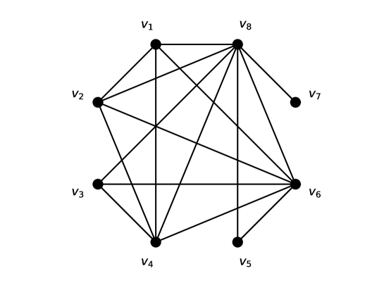
Figure 1. The connected anti-regular graph $A_{8}$ in the canonical labeling

As will be seen, a distinct labeling of the vertex set of $A_{n}$ results in a block structure for $A$. Let $J=J_{k}$ denote the $k\times k$ all ones matrix and let $I=I_{k}$ denote the $k\times k$ identity matrix.

Lemma 4.1.

The adjacency matrix of $A_{2k}$ can be written as

(4) $$A=\begin{pmatrix}0&B\\[8.61108pt] B&J-I\end{pmatrix}$$

where $B$ is the $k\times k$ Hankel matrix

$$B=\begin{pmatrix}&&&&1\\ &&&\iddots&1\\ &&\iddots&\iddots&\vdots\\ &\iddots&\iddots&&\vdots\\ 1&1&\cdots&\cdots&1\end{pmatrix}.$$

Proof.

Recall that $A_{n}$ is the unique connected graph on $n$ vertices that has exactly only two vertices of the same degree. Moreover, it is known [2] that the repeated degree of $A_{2k}$ is $k$, that is, the degree sequence of $A_{2k}$ in non-increasing order is

(5) $$d(A_{n})=\left(n-1,n-2,\ldots,\frac{n}{2},\frac{n}{2},\frac{n}{2}-1,\ldots,2,1\right).$$

It is clear that the degree sequence of the graph with adjacency matrix (4) is also (5). Since $A_{n}$ is uniquely determined by its degree sequence the claim holds. ∎

Remark 4.1.

Starting with the canonically labelled vertex set of $A_{n}$, the permutation

(6) $$\sigma=\begin{pmatrix}v_{1}&v_{2}&v_{3}&\ldots&v_{n-2}&v_{n-1}&v_{n}\\ v_{\frac{n}{2}}&v_{\frac{n}{2}+1}&v_{\frac{n}{2}-1}&\ldots&v_{n-1}&v_{1}&v_{n}\end{pmatrix}$$

relabels the vertices of $A_{n}$ so that its adjacency matrix is transformed from (3) to (4) via the permutation matrix associated to $\sigma$. The newly labelled graph is such that $\textup{deg}(v_{i})\leq\textup{deg}(v_{i+1})$. For example, when $n=8$ the adjacency matrix (4) is

$$A=\begin{pmatrix}0&0&0&0&0&0&0&1\\ 0&0&0&0&0&0&1&1\\ 0&0&0&0&0&1&1&1\\ 0&0&0&0&1&1&1&1\\ 0&0&0&1&0&1&1&1\\ 0&0&1&1&1&0&1&1\\ 0&1&1&1&1&1&0&1\\ 1&1&1&1&1&1&1&0\end{pmatrix}.$$

To study the eigenvalues of $A$ we will obtain an eigenvalue equation for $A^{-1}$. Expressions for $A^{-1}$ involving sums of certain matrices are known when the vertex set of $A_{n}$ is canonically labelled [1]. On the other hand, our choice of vertex labels for $A_{n}$ produces a closed-form expression for $A^{-1}$. The proof of the following is left as a straightforward computation.

Lemma 4.2.

Consider the adjacency matrix (4) of $A_{n}$ where $n=2k$. Then

$$A^{-1}=\begin{pmatrix}V&W\\[8.61108pt] W&0\end{pmatrix}$$

where $W=B^{-1}$ and $V=-B^{-1}(J-I)B^{-1}$. Explicitly,

$$W=\begin{pmatrix}&&&-1&1\\ &&\iddots&\iddots&\\ &\iddots&\iddots&&\\ -1&\iddots&&&\\ 1&&&&\end{pmatrix}\quad\textup{ and }\quad V=\begin{pmatrix}2&-1&&&\\ -1&\ddots&\ddots&&\\ &\ddots&\ddots&\ddots&\\ &&\ddots&2&-1\\ &&&-1&0\end{pmatrix}.$$

Notice that $W$ is a Hankel matrix and the $(k-1)\times(k-1)$ leading principal submatrix of $V$ is a tridiagonal Toeplitz matrix.

Example 4.2.

For our running example when $n=8$ we have

$$A^{-1}=\begin{pmatrix}V&W\\[8.61108pt] W&0\end{pmatrix}=\begin{pmatrix}2&-1&0&0&0&0&-1&1\\ -1&2&-1&0&0&-1&1&0\\ 0&-1&2&-1&-1&1&0&0\\ 0&0&-1&0&1&0&0&0\\ 0&0&-1&1&0&0&0&0\\ 0&-1&1&0&0&0&0&0\\ -1&1&0&0&0&0&0&0\\ 1&0&0&0&0&0&0&0\end{pmatrix}.$$

5. The eigenvalues of $A_{n}$

Suppose that $z=(x,y)\in\mathbb{R}^{2k}$ is an eigenvector of $A^{-1}$ with eigenvalue $\alpha\in\mathbb{R}$, where $x,y\in\mathbb{R}^{k}$. From $A^{-1}z=\alpha z$ we obtain the two equations

$$Vx+Wy =\alpha x$$

$$Wx =\alpha y$$

and after substituting $y=\tfrac{1}{\alpha}Wx$ into the first equation and re-arranging we obtain

$$(\alpha^{2}I-\alpha V-W^{2})x=0.$$

Clearly, we must have $x\neq 0$. Let $R(\alpha)=\alpha^{2}I-\alpha V-W^{2}$ so that $\det(R(t))=\det(tI-A^{-1})$ is the characteristic polynomial of $A^{-1}$. It is straightforward to verify that

$$R(\alpha)=\begin{pmatrix}f(\alpha)&\alpha+1&&&\\ \alpha+1&\ddots&\ddots&&\\ &\ddots&\ddots&\ddots&\\ &&\ddots&f(\alpha)&\alpha+1\\ &&&\alpha+1&\alpha^{2}-1\end{pmatrix}$$

where $f(\alpha)=\alpha^{2}-2\alpha-2$. Since it is already known that $\alpha=-1$ is an eigenvalue of $A^{-1}$ (this can easily be seen from the last column or row of $R(\alpha)$), we consider instead the matrix

$$S(\alpha)=\frac{1}{(\alpha+1)}R(\alpha)=\begin{pmatrix}h(\alpha)&1&&&\\ 1&\ddots&\ddots&&\\ &\ddots&\ddots&\ddots&\\ &&\ddots&h(\alpha)&1\\ &&&1&\alpha-1\end{pmatrix}$$

where $h(\alpha)=\frac{\alpha^{2}-2\alpha-2}{\alpha+1}$. Hence, $\alpha\neq-1$ is an eigenvalue of $A^{-1}$ if and only if $\det(S(\alpha))=0$. We now obtain a recurrence relation for $\det(S(\alpha))$. To that end, notice that the $(k-1)\times(k-1)$ leading principal submatrix of $S(\alpha)$ is a tridiagonal Toeplitz matrix. Hence, for $m\geq 1$ define

$$\phi_{m}(\alpha)=\det\begin{pmatrix}h(\alpha)&1&&\\ 1&\ddots&\ddots&\\ &\ddots&\ddots&1\\ &&1&h(\alpha)\end{pmatrix}_{m\times m}.$$

A straightforward Laplace expansion of $\det(S(\alpha))$ along the last row yields

$$\det(S(\alpha))=(\alpha-1)\phi_{k-1}(\alpha)-\phi_{k-2}(\alpha).$$

Hence, $\alpha\neq-1$ is an eigenvalue of $A^{-1}$ if and only if

$$(\alpha-1)\phi_{k-1}(\alpha)-\phi_{k-2}(\alpha)=0.$$

On the other hand, for $m\geq 2$ the Laplace expansion of $\phi_{m}(\alpha)$ along the last row produces the recurrence relation

$$\phi_{m}(\alpha)=h(\alpha)\phi_{m-1}(\alpha)-\phi_{m-2}(\alpha)$$

with $\phi_{0}(\alpha)=1$ and $\phi_{1}(\alpha)=h(\alpha)$. We can therefore conclude that $\phi_{m}(\alpha)=U_{m}\Big{(}\frac{h(\alpha)}{2}\Big{)}$ and thus $\alpha\neq-1$ is an eigenvalue of $A^{-1}$ if and only if

(7) $$(\alpha-1)U_{k-1}\left(\frac{h(\alpha)}{2}\right)-U_{k-2}\left(\frac{h(\alpha)}{2}\right)=0.$$

Substituting $\alpha=\frac{1}{\lambda}$ into (7) and re-arranging yields

$$\lambda=\frac{U_{k-1}(\beta(\lambda))}{U_{k-1}(\beta(\lambda))+U_{k-2}(\beta(\lambda))}$$

where $\beta(\lambda)=\frac{h(1/\lambda)}{2}=\frac{1-2\lambda-2\lambda^{2}}{2\lambda(\lambda+1)}$. Recalling the definition (1) of $U_{m}(x)$, we have proved the following.

Theorem 5.1.

Let $n=2k$ and let $A_{n}$ denote the connected anti-regular graph with $n$ vertices. Then $\lambda$ is an eigenvalue of $A_{n}$ if and only if

(8) $$\lambda=\frac{\sin(k\theta)}{\sin(k\theta)+\sin((k-1)\theta)}$$

where $\theta=\arccos\left(\frac{1-2\lambda-2\lambda^{2}}{2\lambda(\lambda+1)}\right)$.

Remark 5.1.

In [6, Theorem 3], recurrence relations for the characteristic polynomial of the adjacency matrix of $A_{n}$ involving Chebyshev polynomials are obtained using combinatorial methods.

We now analyze the character of the solution set of (8). To that end, first define the function

$$\theta(\lambda)=\arccos\left(\frac{1-2\lambda-2\lambda^{2}}{2\lambda(\lambda+1)}\right).$$

Using the fact that the domain and range of $\arccos$ is $[-1,1]$ and $[0,\pi]$, respectively, it is straightforward to show that the domain and range of $\theta(\lambda)$ is $(-\infty,\tfrac{-1-\sqrt{2}}{2}]\cup[\tfrac{-1+\sqrt{2}}{2},\infty)$ and $[0,\pi)$, respectively. The graph of $\theta(\lambda)$ is displayed in Figure 2.

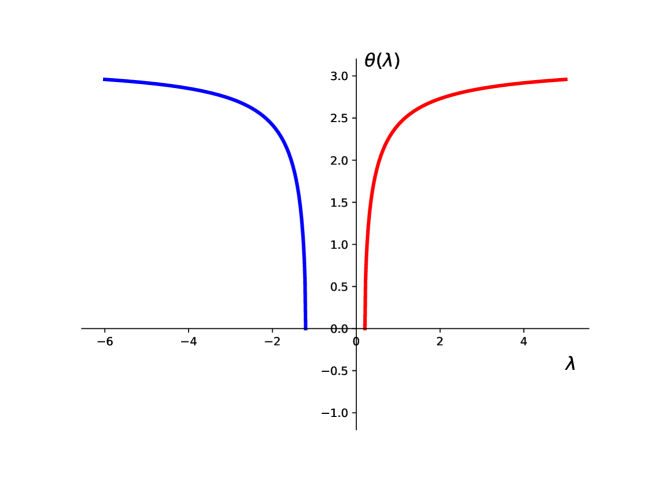
Figure 2. Graph of the function $\theta(\lambda)=\arccos\left(\frac{1-2\lambda^{2}-2\lambda}{2\lambda(\lambda+1)}\right)$ on its domain $(-\infty,\tfrac{-1-\sqrt{2}}{2}]\cup[\tfrac{-1+\sqrt{2}}{2},\infty)$

Next, define the function

(9) $$F(\theta)=\frac{\sin(k\theta)}{\sin(k\theta)+\sin((k-1)\theta)}.$$

In the interval $(0,\pi)$, the function $F$ has vertical asymptotes at

$$\gamma_{j}=\frac{2j\pi}{2k-1},\quad j=1,2,\ldots,k-1.$$

This follows from the trigonometric identity

$$\sin(k\theta)+\sin((k-1)\theta)=2\sin{\frac{(2k-1)\theta}{2}}\cos{\frac{\theta}{2}}.$$

For notational consistency we define $\gamma_{0}=0$. Hence, $F$ is continuously differentiable on the set $(0,\gamma_{1})\cup(\gamma_{1},\gamma_{2})\cup\cdots(\gamma_{k},\pi)$. Moreover, using l’Hópital’s rule it is straightforward to show that

$$\lim_{\theta\rightarrow 0}F(\theta)=\frac{k}{2k-1}$$

and

$$\lim_{\theta\rightarrow\pi}F(\theta)=k.$$

Hence, there is no harm in defining $F(0)=\frac{k}{2k-1}$ and $F(\pi)=k$ so that we can take $D=[0,\gamma_{1})\cup(\gamma_{1},\gamma_{2})\cup\cdots\cup(\gamma_{k-1},\pi]$ as the domain of continuity of $F$.

We can now prove Theorem 2.1.

Proof of Theorem 2.1.

The domain of $\theta(\lambda)$ does not contain any point in the interior of $\Omega$ and therefore no solution of (8) is in the interior of $\Omega$. At the boundary points of $\Omega$ we have

$$\theta(\tfrac{-1-\sqrt{2}}{2})=\theta(\tfrac{-1+\sqrt{2}}{2})=0.$$

On the other hand, $F(0)=\tfrac{k}{2k-1}$ and thus the boundary points of $\Omega$ are not solutions to (8) either. The case that $n$ is odd is similar and will be dealt with in Section 7. ∎

We now analyze solutions to (8) by treating $\theta$ as the unknown variable and expressing $\lambda$ in terms of $\theta$. To that end, solving for $\lambda$ from the equation $\theta=\arccos\left(\frac{1-2\lambda^{2}-2\lambda}{2\lambda(\lambda+1)}\right)$ yields the two solutions

(10) $$\lambda=f_{1}(\theta) =\frac{-(\cos\theta+1)+\sqrt{(\cos\theta+1)(\cos\theta+3)}}{2(\cos\theta+1)}$$

$$\lambda=f_{2}(\theta) =\frac{-(\cos\theta+1)-\sqrt{(\cos\theta+1)(\cos\theta+3)}}{2(\cos\theta+1)}.$$

Notice that

(11) $$f_{1}(\theta)+f_{2}(\theta)=-1,$$

a fact that will be used to show the bipartite character of large anti-regular graphs. Both $f_{1}$ and $f_{2}$ are continuous on $[0,\pi)$, continuously differentiable on $(0,\pi)$, and $\lim_{\theta\rightarrow\pi^{-}}f_{1}(\theta)=\infty$ and $\lim_{\theta\rightarrow\pi^{-}}f_{2}(\theta)=-\infty$. In Figures 3-4, we plot the functions $f_{1}(\theta),f_{2}(\theta)$, and $F(\theta)$ for the values $k=8$ and $k=16$ in the interval $0\leq\theta\leq\pi$. A dashed line at the value $\lambda=-\tfrac{1}{2}=\frac{f_{1}(\theta)+f_{2}(\theta)}{2}$ is included to emphasize that it is a line of symmetry between the graphs of $f_{1}$ and $f_{2}$.

Figures 3-4 show that the graphs of $F$ and $f_{1}$ intersect exactly $k$ times, say at $\theta^{+}_{1},\ldots,\theta^{+}_{k}$, and thus $\lambda^{+}_{j}=f_{1}(\theta^{+}_{j})$ for $j=1,2,\ldots,k$ are the positive eigenvalues of $A_{n}$. Similarly, $F$ and $f_{2}$ intersect exactly $(k-1)$ times, say at $\theta^{-}_{1},\ldots,\theta^{-}_{k-1}$, and thus $\lambda^{-}_{j}=f_{2}(\theta^{-}_{j})$ for $j=1,2,\ldots,k-1$ are the negative eigenvalues of $A_{n}$ besides the eigenvalue $\lambda=-1$. The following theorem formalizes the above observations and supplies interval estimates for the eigenvalues.

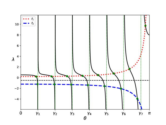
Figure 3. Graph of the functions $f_{1}(\theta),f_{2}(\theta)$, and $F(\theta)$ (black) for $\theta\in[0,\pi]$ for $k=8$

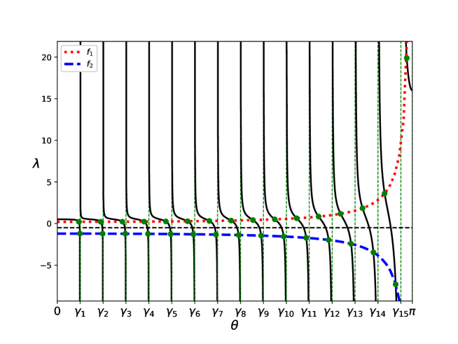
Figure 4. Graph of the functions $f_{1}(\theta),f_{2}(\theta)$, and $F(\theta)$ (black) for $\theta\in[0,\pi]$ for $k=16$

Theorem 5.2.

Let $A_{n}$ be the connected anti-regular graph with $n=2k$ vertices. Let $F(\theta)$ be defined as in (9) and let $f_{1}(\theta)$ and $f_{2}(\theta)$ be defined as in (10), and recall that $\gamma_{j}=\frac{2\pi j}{2k-1}$ for $j=0,1,\ldots,k-1$.

1. The functions $F(\theta)$ and $f_{1}(\theta)$ intersect exactly $k$ times in the interval $0<\theta<\pi$. If $\theta^{+}_{1}<\theta^{+}_{2}<\cdots<\theta^{+}_{k}$ are the intersection points then the positive eigenvalues of $A_{n}$ are

   $$f_{1}(\theta^{+}_{1})<f_{1}(\theta^{+}_{2})<\cdots<f_{1}(\theta^{+}_{k}).$$

   Moreover, for $j=1,2,\ldots,k-1$ it holds that

   $$f_{1}(\gamma_{j-1})<f_{1}(\theta^{+}_{j})<f_{1}(\gamma_{j}).$$

2. The functions $F(\theta)$ and $f_{2}(\theta)$ intersect exactly $(k-1)$ times in the interval $0<\theta<\pi$. If $\theta^{-}_{1}<\theta^{-}_{2}<\cdots<\theta^{-}_{k-1}$ are the intersection points then the negative eigenvalues of $A_{n}$ are

   $$f_{2}(\theta^{-}_{k-1})<\cdots<f_{2}(\theta^{-}_{2})<f_{2}(\theta^{-}_{1})<-1.$$

   Moreover, for $j=1,2,\ldots,k-1$ it holds that

   $$f_{2}(\gamma_{j})<f_{2}(\theta^{-}_{j})<f_{2}(\gamma_{j-1}).$$

Proof.

One computes that

$$f_{1}^{\prime}(\theta)=\frac{\sin\theta}{2(\cos\theta+1)\sqrt{(\cos\theta+1)(\cos\theta+3)}}$$

and thus $f_{1}^{\prime}(\theta)>0$ for $\theta\in(0,\pi)$. Therefore, $f_{1}$ is strictly increasing on the interval $(0,\pi)$. Since $f_{2}(\theta)=-1-f_{1}(\theta)$ it follows that $f_{2}$ is strictly decreasing on the interval $(0,\pi)$. On the other hand, using basic trigonometric identities and the relation $\sin(\theta)U_{k-1}(\cos\theta)=\sin(k\theta)$, we compute that

$$F^{\prime}(\theta) =\frac{\left[-k+U_{k-1}(\cos\theta)\cos((k-1)\theta)\right]\sin\theta}{[\sin(k\theta)+\sin((k-1)\theta)]^{2}}.$$

It is known that $\max_{x\in[-1,1]}|U_{m}(x)|=(m+1)$ and the maximum occurs at $x=\pm 1$ [8]. Therefore, $F^{\prime}(\theta)<0$ for all $\theta\in D\backslash\{0,\pi\}$. It follows that $F$ is a strictly decreasing function on $D$, and when restricted to the interval $(\gamma_{j},\gamma_{j+1})$ for any $j=1,\ldots,k-2$, $F$ is a bijection onto $(-\infty,\infty)$. Now, since $f_{1}$ is a strictly increasing continuous function on $[\gamma_{j},\gamma_{j+1}]$ for $j=1,2,\ldots,k-2$, the graphs of $F$ and $f_{1}$ intersect at exactly one point inside the interval $(\gamma_{j},\gamma_{j+1})$. A similar argument applies to $f_{2}$ and $F$ on each interval $(\gamma_{j},\gamma_{j+1})$ for $j=1,2,\ldots,k-2$. Now consider the leftmost interval $[0,\gamma_{1})$. We have that $f_{1}(0)<F(0)$ and since $f_{1}$ is strictly increasing and continuous on $[0,\gamma_{1}]$, and $F$ is strictly decreasing and $\lim_{\theta\rightarrow\gamma_{1}^{-}}F(\theta)=-\infty$, $F$ and $f_{1}$ intersect only once in the interval $(0,\gamma_{1})$. A similar argument holds for $f_{2}$ and $F$ on the interval $(0,\gamma_{1})$. Finally, on the interval $(\gamma_{k-1},\pi]$, we have $f_{2}(\gamma_{k-1})<F(\pi)$ and since $f_{2}$ decreases and $F$ is strictly increasing on the interval $(\gamma_{k-1},\pi)$ then $f_{2}$ and $F$ do not intersect there. On the interval $(\gamma_{k-1},\pi)$, $f_{1}$ has vertical asymptote at $\theta=\pi$ and is strictly increasing and $F$ is continuous and decreasing on $(\gamma_{k-1},\pi]$. Thus, in $(\gamma_{k-1},\pi]$, $f_{1}$ and $F$ intersect only once. This completes the proof. ∎

Theorem 2.2 now follows from the fact that $\lim_{k\rightarrow\infty}f_{1}(\theta^{+}_{1})=f_{1}(0)=\frac{-1+\sqrt{2}}{2}$ and that $\lim_{k\rightarrow\infty}f_{2}(\theta^{-}_{1})=f_{2}(0)=\frac{-1-\sqrt{2}}{2}$. We also obtain the following corollary.

Corollary 5.1.

Let $\lambda_{\textup{max}}>0$ and $\lambda_{\textup{min}}<0$ denote the largest and smallest eigenvalues, respectively, of the connected anti-regular graph $A_{n}$ where $n$ is even. Then

$$F(\pi)=\frac{n}{2}<\lambda_{\textup{max}}$$

and

$$f_{2}\left(\tfrac{2(n/2-1)\pi}{n-1}\right)<\lambda_{\textup{min}}.$$

Through numerical experiments, we have determined that the mid-point of the interval $(\gamma_{k-1},\pi)$, which is $\frac{(4k-3)\pi}{2(2k-1)}$, is a good approximation to $\theta^{+}_{k}\in(\gamma_{k-1},\pi)$, that is,

$$\lambda_{\textup{max}}\approx F\left(\frac{(4k-3)\pi}{2(2k-1)}\right).$$

In Table 1 we show the results of computing the ratio $t_{k}=\frac{(\theta^{+}_{k}-\gamma_{k-1})}{(\pi-\gamma_{k-1})}$ for $k=125,250,\ldots,32000$ which shows that possibly $\lim_{k\rightarrow\infty}t_{k}=\tfrac{1}{2}$.

$n=2k$	$t_{k}$
250	0.5020031290
500	0.5010007838
1000	0.5005001962
2000	0.5002500492
4000	0.5001250123
8000	0.5000625018
16000	0.5000312567
32000	0.5000156204

Table 1. The ratio $t_{k}=\frac{(\theta^{+}_{k}-\gamma_{k-1})}{(\pi-\gamma_{k-1})}$ for $k=125,250,500,\ldots,32000$

6. The eigenvalues of large anti-regular graphs

A graph $G$ is called bipartite if there exists a partition $\{X,Y\}$ of the vertex set $V(G)$ such that any edge of $G$ contains one vertex in $X$ and the other in $Y$. It is known that the eigenvalues of a bipartite graph $G$ are symmetric about the origin. Figures 3-4 reveal that for the connected anti-regular graph $A_{2k}$ a similar symmetry property about the point $-\tfrac{1}{2}$ is approximately true. Specifically, if $\lambda\neq\lambda_{\textup{max}}$ is a positive eigenvalue of $A_{2k}$ then $-1-\lambda$ is approximately an eigenvalue of $A_{2k}$, and moreover the proportion $r\in(0,1)$ of the eigenvalues that satisfy this property to within a given error $\varepsilon>0$ increases as the number of vertices increases.

Recall that if $\lambda^{+}_{1}<\lambda^{+}_{2}<\cdots<\lambda^{+}_{k}$ denote the positive eigenvalues of $A_{2k}$ then there exists unique $\theta^{+}_{1}<\theta^{+}_{2}<\cdots<\theta^{+}_{k}$ in the interval $(0,\pi)$ such that $\lambda^{+}_{j}=f_{1}(\theta^{+}_{j})$, and if $\lambda^{-}_{k-1}<\lambda^{-}_{k-2}<\cdots<\lambda^{-}_{1}<-1$ denote the negative eigenvalues of $A_{2k}$ there exists unique $\theta^{-}_{1}<\theta^{-}_{2}<\cdots<\theta^{-}_{k-1}$ in $(0,\pi)$ such that $\lambda^{-}_{j}=f_{2}(\theta^{-}_{j})$ for $j=1,2,\ldots,k-1$. With this notation we now prove Theorem 2.3.

Proof of Theorem 2.3.

Both $f_{1}(\theta)$ and $f_{2}(\theta)$ are continuous on $[0,\pi)$ and therefore are uniformly continuous on the interval $[0,r\pi]$. Hence, there exists $\delta>0$ such that if $\theta,\gamma\in[0,r\pi]$ and $|\theta-\gamma|<\delta$ then $|f_{1}(\theta)-f_{1}(\gamma)|<\varepsilon/2$ and $|f_{2}(\theta)-f_{2}(\gamma)|<\varepsilon/2$. Let $k$ be such that $\frac{2\pi}{2k-1}\leq\delta$ and let $j^{*}\in\{1,\ldots,k-1\}$ be the largest integer such that $\frac{2j^{*}}{2k-1}\leq r$. Then for all $j\in\{1,\ldots,j^{*}\}$ it holds that $[\gamma_{j-1},\gamma_{j}]\subset[0,r\pi]$. Let $c_{j}\in[\gamma_{j-1},\gamma_{j}]$ be arbitrarily chosen for each $j\in\{1,\ldots,j^{*}\}$. Then $\theta^{+}_{j},\theta^{-}_{j},c_{j}\in[\gamma_{j-1},\gamma_{j}]$ implies that $|f_{1}(\theta^{+}_{j})-f_{1}(c_{j})|<\varepsilon/2$ and $|f_{2}(\theta^{-}_{j})-f_{2}(c_{j})|<\varepsilon/2$ for $j\in\{1,\ldots,j^{*}\}$. Therefore, if $j\in\{1,\ldots,j^{*}\}$ then

$$|\lambda^{+}_{j}+\lambda^{-}_{j}+1| =|f_{1}(\theta^{+}_{j})+f_{2}(\theta^{-}_{j})+1|$$

$$=|f_{1}(\theta^{+}_{j})-f_{1}(c_{j})+f_{1}(c_{j})+f_{2}(\theta^{-}_{j})-f_{2}(c_{j})+f_{2}(c_{j})+1|$$

$$\leq|f_{1}(\theta^{+}_{j})-f_{1}(c_{j})|+|f_{2}(\theta^{-}_{j})-f_{2}(c_{j})|+|f_{1}(c_{j})+f_{2}(c_{j})+1|$$

$$=|f_{1}(\theta^{+}_{j})-f_{1}(c_{j})|+|f_{2}(\theta^{-}_{j})-f_{2}(c_{j})|$$

$$<\varepsilon$$

where we used the fact that $f_{1}(c_{j})+f_{2}(c_{j})+1=0$. This completes the proof for the even case. As discussed in Section 7, the odd case is similar. ∎

Note that the proportion of $j\in\{1,2,\ldots,k-1\}$ such that $\tfrac{2j}{2k-1}\leq r$ is approximately $r$. In the next theorem we obtain estimates for $|\lambda^{+}_{j}+\lambda^{-}_{j}+1|$ using the Mean Value theorem.

Theorem 6.1.

Let $A_{n}$ be the connected anti-regular graph where $n=2k$. Then for all $1\leq j\leq k-1$ it holds that

$$|\lambda^{+}_{j}+\lambda^{-}_{j}+1|\leq\frac{4\pi f_{1}^{\prime}(\gamma_{j})}{2k-1}.$$

In particular, for fixed $r\in(0,1)$ and a given arbitrary $\varepsilon>0$, if $k$ is such that $\frac{4\pi f_{1}^{\prime}(r\pi)}{2k-1}<\varepsilon$ then

$$|\lambda^{+}_{j}+\lambda^{-}_{j}+1|<\varepsilon$$

for all $1\leq j\leq\frac{(2k-1)r}{2}$.

Proof.

First note that since $f_{1}(\theta)+f_{2}(\theta)=-1$ it follows that $f_{2}^{\prime}(\theta)=-f_{1}^{\prime}(\theta)$. The derivative $f^{\prime}_{1}$ vanishes at $\theta=0$, is non-negative and strictly increasing on $[0,\pi)$. Therefore, by the Mean value theorem, on any closed interval $[a,b]\subset[0,\pi)$, both $f_{1}(\theta)$ and $f_{2}(\theta)$ are Lipschitz with constant $K=f_{1}^{\prime}(b)$. Hence, a similar computation as in the proof of Theorem 2.3 shows that

$$|\lambda^{+}_{j}+\lambda^{-}_{j}+1|\leq\frac{4\pi f_{1}^{\prime}(\gamma_{j})}{2k-1}$$

for $j=1,2,\ldots,k-1$. Therefore, if $k$ is such that $\frac{4\pi f_{1}^{\prime}(r\pi)}{2k-1}<\varepsilon$ then for $1\leq j\leq\frac{(2k-1)r}{2}$ we have that $\frac{2\pi j}{2k-1}\leq r\pi$ and therefore

$$|\lambda^{+}_{j}+\lambda^{-}_{j}+1|\leq\frac{4\pi f_{1}^{\prime}(\gamma_{j})}{2k-1}\leq\frac{4\pi f_{1}^{\prime}(r\pi)}{2k-1}<\varepsilon.$$

∎

A similar proof gives the following estimates for the eigenvalues with error bounds.

Theorem 6.2.

Let $A_{n}$ be the connected anti-regular graph where $n=2k$. For $1\leq j\leq k-1$ it holds that

$$|\lambda^{+}_{j}-f_{1}(\gamma_{j})|\leq\frac{2\pi f_{1}^{\prime}(\gamma_{j})}{2k-1}$$

and

$$|\lambda^{-}_{j}-f_{2}(\gamma_{j})|\leq\frac{2\pi f_{1}^{\prime}(\gamma_{j})}{2k-1}.$$

We now prove Theorem 2.4.

Proof of Theorem 2.4.

It is clear that $\{-1,0\}\subset\sigma\subset\bar{\sigma}$. Let $\varepsilon>0$ be arbitrary and let $y\in[\tfrac{-1+\sqrt{2}}{2},\infty)$. Then $y\in\bar{\sigma}$ if there exists $\mu\in\sigma$ such that $|\mu-y|<\varepsilon$. If $y\in\sigma$ the result is trivial, so assume that $y\not\in\sigma$. Since $f_{1}:[0,\pi)\rightarrow[\tfrac{-1+\sqrt{2}}{2},\infty)$ is a bijection, there exists a unique $\theta^{\prime}\in[0,\pi)$ such that $y=f_{1}(\theta^{\prime})$. Let $c\in[0,\pi)$ be such that $\theta^{\prime}<c<\pi$. For $k$ sufficiently large, there exists $j\in\{1,\ldots,k-1\}$ such that $\theta^{\prime}\in[\gamma_{j-1},\gamma_{j}]$ and $\tfrac{2j\pi}{2k-1}\leq c$. Increasing $k$ if necessary, we can ensure that also $\frac{2\pi f_{1}^{\prime}(c)}{2k-1}<\varepsilon$. Then by the Mean value theorem applied to $f_{1}$ on the interval $I=[\min\{\theta^{\prime},\theta^{+}_{j}\},\max\{\theta^{\prime},\theta^{+}_{j}\}]$, there exists $c_{j}\in I$ such that

$$|\lambda^{+}_{j}-y|=|f_{1}(\theta^{+}_{j})-f_{1}(\theta^{\prime})|\leq|\theta^{+}_{j}-\theta^{\prime}|f_{1}^{\prime}(c_{j})<\frac{2\pi}{2k-1}f_{1}^{\prime}(c)<\varepsilon,$$

where in the penultimate inequality we used the fact that $f_{1}^{\prime}$ is increasing and $c_{j}<c$. This proves that $y$ is a limit point of $\sigma$ and thus $y\in\bar{\sigma}$. A similar argument can be performed in the case that $y\in(-\infty,\tfrac{-1-\sqrt{2}}{2}]$ using $f_{2}$. ∎

7. The odd case

In this section, we give an overview of the details for the case that $A_{n}$ is the unique connected anti-regular graph with $n=2k+1$ vertices. In the canonical labeling of $A_{n}$, the partition $\pi=\{\{v_{1},v_{2}\},\{v_{3}\},\{v_{4}\},\ldots,\{v_{n}\}\}=\{C_{1},C_{2},\ldots,C_{2k}\}$ is an equitable partition of $A_{n}$ [14]. In other words, $\pi$ is the degree partition of $A_{n}$ (we note that this is true for any threshold graph). The quotient graph $A_{n}/\pi$ has vertex set $\pi$ and its $2k\times 2k$ adjacency matrix is

$$A/\pi=\begin{pmatrix}0&1&0&1&\cdots&0&1\\ 2&0&0&1&\cdots&0&1\\ 0&0&0&1&\cdots&\vdots&\vdots\\ 2&1&1&0&\cdots&\vdots&\vdots\\ \vdots&\vdots&\vdots&\vdots&\ddots&\vdots&\vdots\\ 0&\cdots&\cdots&\cdots&\cdots&0&1\\ 2&1&1&\cdots&\cdots&1&0\end{pmatrix}.$$

In other words, $A/\pi$ is obtained from the adjacency matrix of the anti-regular graph $A_{2k}$ (in the canonical labeling) with the $1$’s in the first column replaced by $2$’s. It is a standard result that all of the eigenvalues of $A/\pi$ are eigenvalues of $A_{n}$ [14]. At this point, we proceed just as in Section 4. Under the same permutation (6) of the vertices of $A_{n}/\pi$, the quotient adjacency matrix $A/\pi$ takes the block form

$$A/\pi=\begin{pmatrix}0&B\\[8.61108pt] C&J-I\end{pmatrix}$$

where

$$C=\begin{pmatrix}&&&&2\\ &&&1&2\\ &&\iddots&\vdots&\vdots\\ &\iddots&&\vdots&\vdots\\ 1&1&\cdots&1&2\end{pmatrix}.$$

Then

$$(A/\pi)^{-1}=\begin{pmatrix}-C^{-1}(J-I)B^{-1}&C^{-1}\\[8.61108pt] B^{-1}&0\end{pmatrix}.$$

After computations similar to the even case, the analogue of (7) is

$$\frac{(\alpha^{2}-1/2)}{\alpha+1}U_{k-1}\left(\frac{h(\alpha)}{2}\right)-\frac{1}{2}U_{k-2}\left(\frac{h(\alpha)}{2}\right)=0.$$

After making the substitution $\alpha=\frac{1}{\lambda}$ and simplifying one obtains

$$\frac{(2-\lambda^{2})}{\lambda(\lambda+1)}U_{k-1}(\beta(\lambda))-U_{k-2}(\beta(\lambda))=0$$

or equivalently

$$\frac{(2-\lambda^{2})}{\lambda(\lambda+1)}=\frac{U_{k-2}(\beta(\lambda))}{U_{k-1}(\beta(\lambda))}=\frac{\sin((k-1)\theta)}{\sin(k\theta)}.$$

The analogue of Theorem 5.1 in the odd case is the following.

Theorem 7.1.

Let $n=2k+1$ and let $A_{n}$ denote the connected anti-regular graph with $n$ vertices. Then $\lambda\neq 0$ is an eigenvalue of $A_{n}$ if and only if

(12) $$\frac{(2-\lambda^{2})}{\lambda(\lambda+1)}=\frac{\sin((k-1)\theta)}{\sin(k\theta)}$$

where $\theta=\arccos\left(\frac{1-2\lambda-2\lambda^{2}}{2\lambda(\lambda+1)}\right)$.

Define the function $g(\lambda)=\frac{(2-\lambda^{2})}{\lambda(\lambda+1)}$. Changing variables from $\lambda$ to $\theta$ as in the even case, and defining $g_{1}(\theta)=g(f_{1}(\theta))$, $g_{2}(\theta)=g(f_{2}(\theta))$, and in this case $F(\theta)=\frac{\sin((k-1)\theta)}{\sin(k\theta)}$, we obtain the two equations

$$g_{1}(\theta) =F(\theta)$$

$$g_{2}(\theta) =F(\theta).$$

The explicit expressions for $g_{1}$ and $g_{2}$ are

$$g_{1}(\theta) =2+3\cos(\theta)+\sqrt{(\cos\theta+1)(\cos\theta+3)}$$

$$g_{2}(\theta) =2+3\cos(\theta)-\sqrt{(\cos\theta+1)(\cos\theta+3)}.$$

The graphs of $g_{1},g_{2}$, and $F$ on the interval $[0,\pi]$ are shown in Figure 5. In this case, the singularities of $F$ occur at the equally spaced points

$$\gamma_{j}=\frac{j\pi}{k},\quad j=1,2,\ldots,k.$$

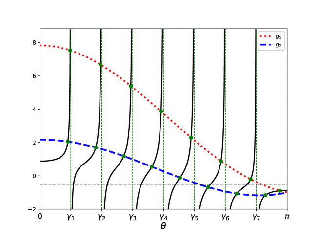
Figure 5. Graph of the functions $g_{1}(\theta),g_{2}(\theta)$, and $F(\theta)$ (black) for $\theta\in[0,\pi]$ for $k=8$

If $\theta_{1}^{+}<\theta^{+}_{2}<\cdots<\theta^{+}_{k}$ denote the unique points where $F$ and $g_{1}$ intersect then $f_{1}(\theta^{+}_{1})<f_{1}(\theta^{+}_{2})<\cdots<f_{1}(\theta^{+}_{k})$ are the positive eigenvalues of $A_{2k+1}$. Similarly, if $\theta_{1}^{-}<\theta^{-}_{2}<\cdots<\theta^{-}_{k}$ denote the unique points where $F$ and $g_{2}$ intersect then $f_{2}(\theta^{-}_{k})<f_{2}(\theta^{-}_{k-1})<\cdots<f_{2}(\theta^{-}_{1})$ are the negative eigenvalues of $A_{2k+1}$.

Theorems 2.1-2.3 hold for the odd case with now $\lambda=0$ being the trivial eigenvalue. Theorem 5.2, Theorem 6.1, and Theorem 6.2 proved for the even case hold almost verbatim for the odd case; the only change is that the ratio $\frac{2\pi}{2k-1}$ is now $\frac{\pi}{k}$.

8. The eigenvalues of threshold graphs

In this section, we discuss how a characterization of the eigenvalues of $A_{n}$ could be used to characterize the eigenvalues of general threshold graphs. Let $G$ be a threshold graph with binary creation sequence $b=(0^{s_{1}},1^{t_{1}},\cdots,0^{s_{k}},1^{t_{k}})$, where $0^{s_{i}}$ is short-hand for $s_{i}\geq 0$ consecutive zeros, and similarly for $1^{t_{i}}$. Let $V(G)=\{v_{1},v_{2},\ldots,v_{n}\}$ denote the associated canonical labeling of $G$ consistent with $b$. The set partition $\pi=\{C_{1},C_{2},\ldots,C_{2k}\}$ of $V(G)$ where $C_{1}$ contains the first $s_{1}$ vertices, $C_{2}$ contains the next $t_{1}$ vertices, and so on, is an equitable partition of $G$. The $2k\times 2k$ quotient graph $G/\pi$ has adjacency matrix

$$A_{\pi}=A_{2k}+\operatorname{diag}(0,\beta_{1},\ldots,0,\beta_{k})$$

where $A_{2k}$ is the adjacency matrix of the connected anti-regular graph with $2k$ vertices and $\beta_{i}=1-\frac{1}{t_{i}}$, see for instance [13]. The eigenvalues of $G$ other than the trivial eigenvalues $\lambda=-1$ and/or $\lambda=0$ are exactly the eigenvalues of $A_{\pi}$. Presumably, the characterization of the eigenvalues of $A_{2k}$ that we have done in this paper will be useful in characterizing the eigenvalues of $A_{\pi}$. We leave this investigation for a future paper.

9. Acknowledgements

The authors acknowledge the support of the National Science Foundation under Grant No. ECCS-1700578.

References

[1]
R. Bapat.
On the adjacency matrix of a threshold graph.
Linear Algebra and its Applications, 439(10):3008–3015, 2013.
[2]
M. Behzad and G. Chartrand.
No graph is perfect.
The American Mathematical Monthly, 74(8):962–963, 1967.
[3]
R. Merris.
Antiregular graphs are universal for trees.
Publikacije Elektrotehničkog fakulteta. Serija
Matematika, pages 1–3, 2003.
[4]
N.V.R. Mahadev and U.N. Peled.
Threshold graphs and related topics.Vol. 56. Elsevier, 1995.
[5]
Martin C. Golumbic.
Algorithmic graph theory and perfect graphs.Vol. 57. Elsevier, 2004.
[6]
E. Munarini.
Characteristic, admittance, and matching polynomials of an antiregular graph.
Applicable Analysis and Discrete Mathematics, 3(1):157–176, 2009.
[7]
V.E. Levit and E. Mandrescu.
On the Independence Polynomial of an Antiregular Graph.
Carpathian Journal of Mathematics, 28(2): 279–288, 2012.
[8]
J.C. Mason and D.C. Handscomb.