The Apparent (Gravitational) Horizon in Cosmology

Abstract

In general relativity, a gravitational horizon (more commonly known as the “apparent horizon”) is an imaginary surface beyond which all null geodesics recede from the observer. The Universe has an apparent (gravitational) horizon, but unlike its counterpart in the Schwarzschild and Kerr metrics, it is not static. It may eventually turn into an event horizon—an asymptotically defined membrane that forever separates causally connected events from those that are not—depending on the equation of state of the cosmic fluid. In this paper, we examine how and why an apparent (gravitational) horizon is manifested in the Friedmann-Robertson-Walker metric, and why it is becoming so pivotal to our correct interpretation of the cosmological data. We discuss its observational signature and demonstrate how it alone defines the proper size of our visible Universe. In so doing, we affirm its physical reality and its impact on cosmological models.

I Introduction

The term ‘horizon’ in cosmology is variously used to denote (i) how far particles could have traveled relative to an observer since the big bang (the ‘particle horizon’), or (ii) a two-dimensional surface that forever separates causally connected spacetime events from others that are not (the ‘event horizon’), or (iii) any of several other definitions with a customized application.Rindler:1956 Each has its purpose, though they are sometimes applied incorrectly when using an approach based on conformal diagrams, which are often not as easy to interpret as concepts described in terms of proper distances and times. Part of the difficulty is also that some definitions are based on the use of comoving lengths, while others are written in terms of proper distances. There is no conflict between them, of course, but as the precision of the data increases, it is becoming quite evident that one definition, above all else, appears to be the most relevant to a full appreciation of what the observations are telling us. We shall highlight this particular measure of distance—the ‘apparent’ (or gravitational) horizon—for the majority of this paper, but we shall also compare it to the other horizons in the discussion section towards the end.

Several authors have previously attempted to describe the nature of cosmological expansion and its consequences (e.g., its impact on the redshift of light reaching us from distant sources) using a pedagogical approach, though with various measures of success. Given what we know today, primarily through the extensive database at our disposal, some of which we shall discuss shortly, it is safe to say that a correct understanding of the key observational features in the cosmos is best developed in the context of general relativity. Of course, this introduces the importance of coordinate transformations (and their relevance to how one writes the spacetime metric), the relevance of proper distances and times, and the emergence of the aforementioned horizons due to the finite (and constant) speed of light.

The possibility that a gravitational horizon might exist in the cosmos was considered by Nemiroff and Patla,Nemiroff:2008 who discussed it using a “toy” model based on a Universe dominated by a single, isotropic, stable, static, perfect-fluid energy, though with various levels of pressure. They concluded that the Friedmann equations implied a maximum scale length over which this energy could impact an object gravitationally, but suggested that there is little observational evidence limiting this “gravitational horizon” of our local Universe. The topic of this paper touches on this issue as well, but goes well beyond this early, simple foray into what is—in truth—a much more elaborate physical process, supported by an enormous amount of empirical evidence. We shall learn, e.g., that the gravitational horizon in cosmology coincides with what is commonly referred to as an “apparent” horizon in other applications of general relativity. An excellent discussion on the origin and meaning of apparent horizons may be found in the recent book by Faraoni.Faraoni:2015 A simple definition that serves us well at this early stage is that the apparent horizon separates regions in which null geodesics approach us, from those in which they recede, as measured in terms of the proper distance. Indeed, an early recognition of this dual designation—apparent versus gravitational—was the subject of a paper by Gautreau,Gautreau:1996 who employed a pseudo-Newtonian description of gravity using a Schwarzschild-like curvature spatial coordinate, and showed that light signals reach a maximum distance along their trajectory through the Universe, and then turn around and return to some remote origin. As we shall see shortly, this turning point is closely related to an apparent horizon. We shall argue in this paper that the best way to understand features such as this from a pedagogical standpoint is actually to invoke and utilize the Birkhoff theorem,Birkhoff:1923 an important generalization of Newtonian theory in the general relativistic framework.

In the context of cosmological horizons, the paper by Ellis and Rothman Ellis:1993 was quite useful because, in avoiding unnecessarily complicated presentations, they made it easy to understand how misconceptions often arise from the misinterpretation of coordinate-dependent effects. These authors carefully delineated stationary horizons from apparent horizons, extending in a clear and pedagogical manner the definitions introduced half a century earlier.Rindler:1956

In this paper, we focus our attention on the type of horizon that is not yet commonly known or invoked in the cosmological context—the ‘gravitational horizon’ which, as noted, is typically referred to as the ‘apparent horizon,’ e.g., in a handful of papers dealing specifically with its role in cosmology.Ben-Dov:2007 ; Faraoni:2011 ; Bengtsson:2011 ; Faraoni:2015 As we shall see, this horizon has a radius (the ‘gravitational radius’, $R_{\rm h}$) that coincides with the much better known radius of the Hubble sphere. In fact, the very existence of a Hubble radius is due to the presence of the gravitational horizon. The former is simply a manifestation of the latter. It is time-dependent—not static like its counterpart in the Schwarzschild and Kerr metrics—and may, or may not, eventually turn into an event horizon in the asymptotic future, depending on the equation of state of the cosmic fluid. (Later in this paper, we shall directly compare the particle, event, and gravitational horizons with each other.) Ironically, though introduced in ref. Melia:2007 , an unrecognized form of $R_{\rm h}$ actually appeared a century ago in de Sitter’s deSitter:1917 own account of his spacetime metric, but the choice of coordinates for which $R_{\rm h}$ appears in his metric coefficients eventually fell out of favour following the introduction of comoving coordinates in the 1920’s (principally by Friedmann,Friedmann:1923 ) which have been used ever since in cosmological applications. We shall see shortly how these two forms of the metric are related to each other.

As of today, however, there is still some confusion concerning the properties of $R_{\rm h}$ and how it affects our cosmological observations. The time-dependent gravitational horizon need not be a null surface, but is often confused with one. It has sometimes been suggested Davis:2004 ; vanOirschot:2010 ; Lewis:2013 ; Kim:2018 that sources beyond $R_{\rm h}(t_{0})$ are observable today, which is absolutely not the case.Bikwa:2012 ; Melia:2012 ; Melia:2013 Much of this debate appears to be due to a confusion between proper and coordinate speeds in general relativity. Simply put, there is no limit on the coordinate speed, which may exceed the speed of light $c$, but there is absolutely a limit on the proper (or physical) speed, whose determination must include the curvature-dependent metric coefficients. When this distinction is ignored or unrecognized, it can lead to a possibly alarming conclusion that recessional velocities in the cosmos can exceed $c$ even within the particle horizon of the observer.Stuckey:1992 As ref. Davis:2001 explains, this “superluminal” recession is even claimed on occasion to be a contradiction of special relativity, which some rationalize by explaining that the limiting speed $c$ is only valid within a non-expanding space, while the expansion may create superluminal motion.Kaya:2011 The aforementioned distinction between coordinate and proper speeds completely removes any such ambiguous (and sometimes incorrect) statements.Melia:2013 Our development of $R_{\rm h}$ in this paper will be fully consistent with such fundamental aspects of the metric in general relativity.

As we shall see shortly, an indication of the role played by $R_{\rm h}$ in our interpretation of the data is suggested by the curious coincidence that $R_{\rm h}(t)=ct$, a rather significant constraint given that the rate at which $R_{\rm h}$ evolves in time is strongly dependent on which components are present in the cosmic fluid.Melia:2003 ; Melia:2007 ; MeliaAbdelqader:2009 ; MeliaShevchuk:2012 ; Melia:2016 ; Melia:2017 Those familiar with black-hole horizons might find this result familiar at first, given that an observer falling freely towards such an object also sees the event horizon approaching him at speed $c$ (so that $\dot{R}_{\rm h}\equiv dR_{\rm h}/dt=c$). But as we shall clarify in this paper, $R_{\rm h}$ is an apparent horizon, not necessarily an event horizon, so its evolution in time depends on the equation of state of the medium. Our principal goal here is therefore to reiterate what the physical meaning of the Universe’s apparent (gravitational) horizon is, to explore its properties in more detail and at greater depth than has been attempted before, and to elucidate its role in establishing the size of the visible Universe based on the subdivision of null geodesics that can, or cannot, physically reach us today (at time $t_{0}$).

Those interested in studying the impact of $R_{\rm h}$ at greater depth may wish to examine how its use eventually resolved the question of whether or not cosmological redshift is due to an effect distinct from the better known kinematic (or Doppler) and gravitational time dilations. This issue has been at the core of a debate between those who claim its origin proves that space is expanding and those who have attempted to demonstrate that it may be calculated without invoking such a poorly understood (and probably unphysical) mechanism.Harrison:1995 ; Chodorowski:2007 ; Chodorowski:2011 ; Baryshev:2008 ; Bunn:2009 ; Cook:2009 ; Gron:2007 A partial demonstration that an interpretation of cosmological redshift as due to the expansion of space is problematic was presented earlier by Bunn and Hogg,Bunn:2009 Cook and Burns,Cook:2009 and Gron and Elgaroy,Gron:2007 but a complete treatmentMelia:2012red proving that it is simply a product of both the Doppler and gravitational redshifts in an expanding cosmos was finalized only after the introduction of the gravitational radius $R_{\rm h}$.

In § 2, we shall briefly introduce the Birkhoff theorem and its corollary, and explain why it is so impactful in helping us understand the relevance of $R_{\rm h}$ to cosmological theory. We shall describe the Friedmann-Robertson-Walker (FRW) metric in § 3, and demonstrate how the concept of a gravitational radius $R_{\rm h}$ emerges from its various forms (based on different choices of the coordinates). In § 4, we shall derive the null geodesic equation, whose properties (and solutions) we study in § 5. We shall see in this section that a comprehensive understanding of how the null geodesics behave leads to a full appreciation of the role of $R_{\rm h}$, which will also help us understand how $R_{\rm h}$ is related to the particle and event horizons in § 6. Finally, we present our conclusions in § 7.

II The Birkhoff Theorem and its Relevance to Cosmology

The concept of a gravitational radius is not as easily implemented in cosmology as it is for, say, a compact star. When matter is distributed within a confined (more or less) spherical volume surrounded by near vacuum, it is straightforward to understand how the gravitational influence of the well-defined mass curves the surrounding spacetime. An apparent (gravitational) horizon appears for the star when its radius is small enough for the escape speed to equal or exceed the speed of light, $c$. The Schwarzschild and Kerr metrics describing the spacetime surrounding such an environment are time-independent, so their apparent (gravitational) horizon is actually an event horizon, and these two terms are often used interchangeably for such objects.

In the cosmological setting, the observations are telling us that the Universe is spatially flat,Planck:2016 meaning that $k=0$ in Equation (3) below, so it will expand forever and is therefore infinite. As observers embedded within it, we do not easily recognize how the gravitational influence of the cosmic fluid varies with distance. But the reason $R_{\rm h}$ is as important an ingredient of the cosmological metric as it is for Schwarzschild or Kerr may be understood in the context of the Birkhoff theorem Birkhoff:1923 and its corollary (see also refs. Weinberg:1972 ; Melia:2007 ). The theorem itself was actually ‘pre-discovered’ by Jebsen a few years earlier,Jebsen:1921 though this work was not as well known until recently.

The Birkhoff theorem is a relativistic generalization of a Newtonian theorem pertaining to spherical mass distributions. It states that for an isotropic distribution of mass-energy, be it static or time-dependent, the surrounding spacetime is described by the Schwarzschild metric. The corollary extends this result in cosmologically important ways, advancing the argument that, for an isotropic Universe, the spacetime curvature a proper distance $R$ relative to any given origin of the coordinates depends solely on the mass-energy content within a sphere of radius $R$; due to spherical symmetry, the rest of the Universe has no influence on the metric at that radius. Many find this confusing because the origin may be placed anywhere in the cosmos, so a radius $R$ for one observer, may be a different radius $R^{\prime}$ for another. The bottom line is that only relative spacetime curvature is relevant in this context. The gravitational influence felt by a test particle at $R$ is relative to an observer at its corresponding origin. For an observer with a different set of coordinates, the relative gravitational influence would, of course, be different. To state this another way, any two points within a medium with non-zero energy density $\rho$ experience a net acceleration (or deceleration) towards (or away) from each other, based solely on how much mass-energy is present between them. This is the reason why the Universe cannot be static, for even though it may be infinite, local motions are dynamically dependent solely on local densities. Ironically, Einstein himself missed this point—and therefore advanced the notion of a steady-state universe—because his thinking on this subject preceded the work of Birkhoff and Jebsen in the 1920’s.

Now imagine the observer extending his perspective to progressively larger radii. Eventually, his sphere of radius $R$ will be large enough (for the given density $\rho$) to create a gravitational horizon. In the next section, we shall prove this rigorously using the Friedmann-Robertson-Walker (FRW) metric, and demonstrate—not surprisingly—that the radius at which this happens, called $R_{\rm h}$ throughout this paper, is simply given by the Schwarzschild form

$$R_{\rm h}={2GM\over c^{2}}\;,$$ (1)

where $M$ is the proper mass contained within a sphere of proper radius $R_{\rm h}$, i.e.,

$$M\equiv{4\pi\over 3}R_{\rm h}^{3}\,{\rho\over c^{2}}\;.$$ (2)

As it turns out, this is also known in some quarters as the Misner-Sharp mass,Misner:1964 defined in the pioneering work of Misner and Sharp on the subject of spherical collapse in general relativity, and sometimes also as the Misner-Sharp-Hernandez mass, to include the later contribution by Hernandez and Misner.Hernandez:1966 ; ProperRadius But unlike the situation with the Schwarzschild and Kerr metrics, the cosmological $R_{\rm h}$ may depend on time, and a sphere with this radius is therefore not necessarily an event horizon. It may turn into one in our asymptotic future, depending on the properties of the cosmic fluid. In either case, however, $R_{\rm h}$ defines a gravitational horizon that, at any cosmic time $t$, separates null geodesics approaching us from those receding, as we shall see more formally in Equation (32) below.

The mass used in Equation (1) is not arbitrary, in the sense that only the Misner-Sharp-Hernandez definition is consistent with the $g_{rr}$ metric coefficient. In a broader context, it is highly non-trivial to identify the physical mass-energy in a non-asymptotically flat geometry in general relativity.Faraoni:2015 With spherical symmetry, however, other possible definitions, such as the Hawking-Hayward quasilocal mass,Prain:2016 reduce exactly to the Misner-Sharp-Hernandez construct. A second example is the Brown-York energy, defined as a two dimensional surface integral of the extrinsic curvature on the two-boundary of a spacelike hypersurface referenced to flat spacetime.Chakraborty:2015

Our derivation of the quantity $R_{\rm h}$, though designed for pedagogy, is nonetheless fully self-consistent with already established knowledge concerning apparent horizons in general relativity, particularly with their application to black-hole systems. An apparent horizon is defined in general, non-spherical, spacetimes by the subdivision of the congruences of outgoing and ingoing null geodesics from a compact, orientable surface. For a spherically symmetric spacetime, these are simply the outgoing and ingoing radial null geodesics from a two-sphere of symmetry.Ben-Dov:2007 ; Faraoni:2011 ; Bengtsson:2011 ; Faraoni:2015 Such a horizon is more practical than stationary event horizons in black-hole systems because the latter require knowledge of the entire future history of the spacetime in order to be located. Apparent horizons are often used in dynamical situations, such as one might encounter when gravitational waves are generated in black-hole merging events.

Unlike the spacetime surrounding compact objects, however, the FRW metric is always spherically symmetric, and therefore the Misner-Sharp-Hernandez mass and apparent horizons are related, as we have found here with our simplified approach based on the Birkhoff theorem and its corollary. Indeed, with spherical symmetry, the general definition of an apparent horizon reduces exactly to Equation (1).Faraoni:2011 ; Faraoni:2015 In other words, the use of Birkhoff’s theorem and its corollary allow us to define a ‘gravitational horizon’ in cosmology which, however, is clearly identified as being the ‘apparent horizon’ defined more broadly, even for systems that are not spherically symmetric. It is therefore appropriate for us to refer to $R_{\rm h}$ as the radius of the apparent horizon in FRW, though given its evident physical meaning, we shall continue to use the designations ‘apparent’ and ‘gravitational’ interchangeably throughout this paper, often combining them (as in ‘apparent (gravitational) horizon’) when referring to the two-dimensional surface it defines.

The impact of $R_{\rm h}$ on our observations and interpretation of the data became quite apparent after the optimization of model parameters in the standard model, $\Lambda$CDM,Bennett:2003 ; Spergel:2003 ; Ade:2014 revealed a gravitational radius $R_{\rm h}(t_{0})$ equal to $ct_{0}$ within the measurement error.Melia:2003 ; Melia:2007 This observed equality cannot be a mere ‘coincidence,’ as some have suggested.Kim:2018 Consider, for example, that in the context of $\Lambda$CDM—a cosmology that ignores the physical reality of $R_{\rm h}$—the equality $R_{\rm h}=ct$ can be achieved only once in the entire (presumably infinite) history of the Universe, making it an astonishingly unlikely event—in fact, if the Universe’s timeline is infinite, the probability of this happening right now, when we happen to be looking, is zero.

There may be several possible explanations for the existence of such a constraint, though the simplest appears to be that $R_{\rm h}$ is always equal to $ct$, in which case this condition would be realized regardless of when the measurements are made. The unlikelihood of measuring a Hubble radius equal to $ct_{0}$ today were these two quantities not permanently linked in general relativity argues for a paramount influence of the apparent (gravitational) horizon in cosmology. In subsequent sections of this paper, we shall describe how and why $R_{\rm h}$ is manifested through the FRW metric. Finally, we shall learn what the photon geodesics in this spacetime are informing us about its geometry.

III The Friedmann-Robertson-Walker Metric

Standard cosmology is based on the Friedmann-Robertson-Walker (FRW) metric for a spatially homogeneous and isotropic three-dimensional space, expanding or contracting as a function of time:

$$ds^{2}=c^{2}\,dt^{2}-a^{2}(t)[dr^{2}(1-kr^{2})^{-1}+r^{2}(d\theta^{2}+\sin^{2}\theta\,d\phi^{2})]\;.$$ (3)

In the coordinates used for this metric, $t$ is the cosmic time, measured by a comoving observer (and is the same everywhere), $a(t)$ is the expansion factor, and $r$ is the comoving radius. The geometric factor $k$ is $+1$ for a closed universe, $0$ for a flat universe, and $-1$ for an open universe.

As we examine the various properties of the FRW metric throughout this paper, we shall see that the coordinates $(ct,r,\theta,\phi)$ represent the perspective of a free-falling observer, analogous to—and fully consistent with—the free-falling observer in the Schwarzschild and Kerr spacetimes. And just as it is sensible and helpful to cast the latter in a form relevant to the accelerated observer as well, e.g., one at rest with respect to the source of gravity, it will be very informative for us to also write the FRW metric in terms of coordinates that may be used to describe a fixed position relative to the observer in the cosmological context.

The proper radius, $R(t)\equiv a(t)r$, is often used to express—not the co-moving distance $r$ between two points but, rather—the changing distance that increases as the Universe expands. This definition of $R$ is actually a direct consequence of Weyl’s postulate,Weyl:1923 which holds that in order for the Cosmological principle to be maintained from one time-slice to the next, no two worldlines can ever cross following the big bang (aside from local peculiar motion that may exist on top of the averaged Hubble flow, of course). To satisfy this condition, every distance in an FRW cosmology must be expressible as the product of a constant comoving length $r$, and a universal function of time, $a(t)$, that does not depend on position. In some situations, $R$ is referred to as the areal radius—the radius of two-spheres of symmetry—defined in a coordinate-independent way by the relation $R\equiv\sqrt{A/4\pi}$, where $A$ is the area of the two-sphere in the symmetry. These two definitions of $R$ are, of course, fully self-consistent with each other.Nielsen:2006 ; Abreu:2010 For example, in this gauge, apparent horizons are located by the constraint $g^{RR}=0$, which is equivalent to the condition $\Phi=0$ in Equations (9) and (10) below.

For convenience, we shall transform the metric in Equation (3) using the definition

$$a(t)=e^{f(t)}\;,$$ (4)

where $f(t)$ is itself a function only of cosmic time $t$.MeliaAbdelqader:2009 And given that current observations indicate a flat universe,Spergel:2003 ; Ade:2014 we shall assume that $k=0$ throughout this paper. Thus, putting

$$r=Re^{-f}\;,$$ (5)

it is straightforward to show that Equation (3) becomes

$$ds^{2}=\left[1-\left(\frac{R\dot{f}}{c}\right)^{2}\right]\,c^{2}\,dt^{2}+2\left(\frac{R\dot{f}}{c}\right)c\,dt\,dR-dR^{2}-R^{2}\,d\Omega^{2}\;,$$ (6)

whereupon, completing the square, one gets

$$ds^{2}=\Phi\left[c\,dt+\left(\frac{R\dot{f}}{c}\right)\Phi^{-1}dR\right]^{2}-\Phi^{-1}{dR^{2}}-R^{2}\,d\Omega^{2}\;,$$ (7)

where

$$d\Omega^{2}\equiv d\theta^{2}+\sin^{2}\theta\,d\phi^{2}\;.$$ (8)

For convenience we have also defined the quantity

$$\Phi\equiv 1-\left(\frac{R\dot{f}}{c}\right)^{2}\;,$$ (9)

which appears frequently in the metric coefficients. We shall rearrange the terms in Equation (7) in order to present the interval in a more standard form:

$$ds^{2}=\Phi\left[1+\left(\frac{R\dot{f}}{c}\right)\Phi^{-1}{\dot{R}\over c}\right]^{2}c^{2}\,dt^{2}-\Phi^{-1}{dR^{2}}-R^{2}\,d\Omega^{2}\;.$$ (10)

In this expression, $\dot{R}$ is to be understood as representing the proper velocity calculated along the worldlines of particular observers, those who have $t$ as their proper time which, as we shall see below, turn out to be the comoving observers.

This metric has much in common with that used to derive the Oppenheimer-Volkoff equations describing the interior structure of a star Oppenheimer:1939 ; Misner:1964 except, of course, that whereas the latter is assumed ab initio to be static, $\dot{R}$ and $\dot{f}$ are functions of time $t$ in a cosmological context. In other words, the Universe is expanding—in general, the FRW metric written in terms of $R$ and $t$ is not static. But there are six special cases where one additional transformation of the time coordinate (from $t$ to an observer-dependent time $T$) does in fact render all of the metric coefficients independent of the new time coordinate $T$.Florides:1980 ; Melia:2013 . These constitute the (perhaps not widely known) FRW metrics with constant spacetime curvature. For reference, we point out that the standard model is not a member of this special set.

A physical interpretation of the factor $\dot{f}/c$ and, indeed, the function $\Phi$ itself, may be found through the use of Birkhoff’s theorem and its corollary which, as we have seen, imply that measurements made by an observer a distance $R$ from his location (at the origin of his coordinates) are unaffected by the mass-energy content of the Universe exterior to the shell at $R$. It is not difficult to show from Equations (9) and (10) that a threshold distance scale is reached when $R\rightarrow R_{\rm h}$, where $R_{\rm h}$ is in fact equal to $c/\dot{f}$. To see this, we note that the FRW metric produces the following equations of motion:

$$H^{2}\equiv\left(\frac{\dot{a}}{a}\right)^{2}=\frac{8\pi G}{3c^{2}}\rho-\frac{kc^{2}}{a^{2}}\;,$$ (11)

$$\frac{\ddot{a}}{a}=-\frac{4\pi G}{3c^{2}}(\rho+3p)\;,$$ (12)

$$\dot{\rho}=-3H(\rho+p)\;,$$ (13)

where an overdot denotes a derivative with respect to $t$, and $\rho$ and $p$ represent, respectively, the total energy density and total pressure in the comoving frame, assuming the perfect fluid form of the stress-energy tensor.

From Equations (1) and (2), one sees that

$$R_{\rm h}^{2}={3c^{4}\over 8\pi G\rho}$$ (14)

which (with the flat condition $k=0$) gives simply

$$R_{\rm h}={c\over H}={ca\over\dot{a}}\;.$$ (15)

That is,

$$R_{\rm h}={c/\dot{f}}\;.$$ (16)

Equation (15) is fully self-consistent with its well-known counterpart in the study of apparent horizons in cosmology, as one may trace with greater detail in refs. Faraoni:2011 ; Faraoni:2015 . Thus, the FRW metric (Equation 10) may also be written in the form

$$ds^{2}=\Phi\left[1+\left(\frac{R}{R_{\rm h}}\right)\Phi^{-1}{1\over c}\dot{R}\right]^{2}c^{2}\,dt^{2}-\Phi^{-1}{dR^{2}}-R^{2}\,d\Omega^{2}\;,$$ (17)

in which the function

$$\Phi\equiv 1-\left(\frac{R}{R_{\rm h}}\right)^{2}$$ (18)

signals the dependence of the coefficients $g_{tt}$ and $g_{RR}$ on the proximity of the proper distance $R$ to the gravitational radius $R_{\rm h}$.

IV Geodesics in FRW

Let us now consider the worldlines of comoving observers. From Weyl’s postulate, we know that

$$\dot{R}=\dot{a}r\;,$$ (19)

which quickly and elegantly leads to Hubble’s law, since

$$\dot{R}={\dot{a}\over a}R\equiv HR\;,$$ (20)

in terms of the previously defined Hubble constant $H$.Hconstant

Therefore, along a (particle) geodesic, the coefficient $g_{tt}$ in Equation (17) simplifies to

$$g_{tt}=\Phi\left[1+\left({R\over R_{\rm h}}\right)^{2}\Phi^{-1}\right]^{2}\;,$$ (21)

which further reduces to the even simpler form

$$g_{tt}=\Phi^{-1}\;.$$ (22)

Thus, the FRW metric for a particle worldline, written in terms of the cosmic time $t$ and the proper radius $R$, is

$$ds^{2}=\Phi^{-1}c^{2}dt^{2}-\Phi^{-1}dR^{2}-R^{2}d\Omega^{2}\;.$$ (23)

And further using the fact that in the Hubble flow

$$dR=c\left({R\over R_{\rm h}}\right)dt\;,$$ (24)

Equation (23) reduces to the final form,

$$ds^{2}=c^{2}dt^{2}-R^{2}d\Omega^{2}\;.$$ (25)

The observer’s metric describing a particle moving radially with the Hubble flow (i.e., with $\dot{R}=HR$ and $d\Omega=0$), is therefore

$$ds=c\,dt\;,$$ (26)

which displays the behavior consistent with the original definition of our coordinates. In particular, the cosmic time $t$ is in fact the proper time measured in the comoving frame anywhere in the Universe, independent of location $R$. In this frame, we are free-falling observers, and our clocks must therefore reveal the local passage of time unhindered by any external gravitational influence.

However, this situation changes dramatically when we examine the behavior of the metric applied to a fixed radius $R=R_{0}$ with respect to the observer. Those familiar with the Schwarzschild and Kerr metrics in black-hole systems will recognize this situation as being analogous to that of an observer maintaining a fixed radius relative to the central source of gravity. The distinction with the previous case is that, whereas $R$ was there associated with particles (e.g., galaxies) expanding with the Hubble flow, we now fix the distance $R_{0}$ and instead imagine particles moving through this point. Since our measurements are now no longer made from the free-falling perspective, we expect by analogy with the Schwarzschild case that gravitational effects must emerge in the metric.

And indeed they do. Returning to Equation (17), we have in this case $dR=0$, so that

$$ds^{2}=\Phi_{0}c^{2}dt^{2}-R^{2}_{0}d\Omega^{2}\;,$$ (27)

and if we again insist on purely radial motion (with $d\Omega^{2}=0$), then the metric takes the form

$$ds^{2}=\Phi_{0}c^{2}dt^{2}\;,$$ (28)

where now $\Phi_{0}\equiv 1-(R_{0}/R_{\rm h})^{2}$. In its elegance and simplicity, this expression reproduces the effects one would have expected by analogy with Schwarzschild and Kerr, in which the passage of time at a fixed proper radius $R_{0}$ is now no longer the proper time in a local free-falling frame. Instead, for any finite interval $ds$, $dt\rightarrow\infty$ as $R_{0}\rightarrow R_{\rm h}$, which endows $R_{\rm h}$ with the same kind of gravitational horizon characteristics normally associated with the Schwarzschild radius in compact objects.

For null geodesics, the situation is quite different, but still fully consistent with the better known behavior one finds in black-hole spacetimes. For a ray of light, $\dot{r}$ cannot be zero, as one may verify directly from the FRW metric in Equation (3). The null condition (i.e., $ds=0$), together with a radial path (and, as always, a flat Universe with $k=0$), leads to the expression

$$c\,dt=\pm a\,dr\;,$$ (29)

which clearly implies that along an inwardly propagating radial null geodesic we must have

$$\dot{r}=-{c\over a}\;.$$ (30)

Thus, in terms of the proper radius $R_{\gamma}$, the motion of light relative to an observer at the origin of the coordinates may be described as

$${dR_{\gamma}\over dt}=\dot{a}r_{\gamma}+a\dot{r}_{\gamma}\;,$$ (31)

or

$${dR_{\gamma}\over dt}=c\left({R_{\gamma}\over R_{\rm h}}-1\right)\;.$$ (32)

In this expression, we have assumed that the ray of light is propagating towards the origin (hence the negative sign). For an outwardly propagating ray which, as we shall see shortly, is relevant to the definition of a ‘particle’ horizon, the minus sign would simply be replaced with $+$. It is trivial to confirm from Equation (17) that replacing $\dot{R}$ with $dR_{\gamma}/dt$ from Equation (32), and putting $dR=(dR_{\gamma}/dt)\,dt$, gives exactly $ds=0$, as required for the radial null geodesic.

This result is hardly surprising, but it demonstrates that regardless of which set of coordinates we use to write the metric for a particle geodesic, either with or without gravitational effects, the behavior of light is always fully consistent with the properties expected of a null geodesic. However, from Equation (32), we learn several new important results. First, $dR_{\gamma}/dt=0$ when $R_{\gamma}=R_{\rm h}$. In other words, the spatial velocity of light measured in terms of the proper distance per unit cosmic time has two components that exactly cancel each other at the gravitational radius. One of these is the propagation of light measured in the comoving frame, where

$${dR_{\gamma\;{\rm com}}\over dt}=-c\;,$$ (33)

while the other is due to the Hubble expansion itself, with

$${dR_{\gamma\;{\rm Hub}}\over dt}=c\left({R_{\gamma}\over R_{\rm h}}\right)\;.$$ (34)

Obviously, given the definition of $R_{\rm h}$, we could have simply written $dR_{\gamma\;{\rm Hub}}/dt=HR_{\gamma}$.

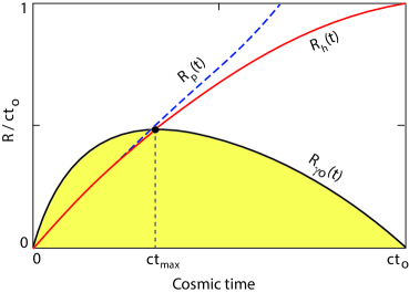
Figure 1: Schematic diagram showing the various measures of distance discussed in the context of an apparent (gravitational) horizon. The solid, black curve shows the null geodesic (i.e., photon trajectory) reaching the observer today, at time $t_{0}$. Only photons emitted along this curve can be seen by us at the present time. The solid, red curve shows the evolution of the gravitational radius $R_{\rm h}(t)$ with time. (This particular illustration pertains to the standard model, $\Lambda$CDM, though the qualitative features are common to most cosmological models.) Prior to the time, $t_{\rm max}$, at which the photon reaches its maximum proper distance relative to the observer, $R_{\gamma 0}$ is greater than $R_{\rm h}$, so according to Equation (32), it must increase with time. This process is reversed at $t_{\rm max}$, however, after which $R_{\gamma 0}<R_{\rm h}$, so that $\dot{R}_{\gamma 0}<0$. Of course, $R_{\gamma 0}\rightarrow 0$ by the time the photon reaches the observer at $t_{0}$. In § 7, we shall also discuss the ‘particle’ horizon, shown here as a dashed blue curve.

Second, we see that when $R_{\gamma}>R_{\rm h}$, the photon’s proper distance actually increases away from us, even though the photon’s velocity is pointed towards the origin as seen in the co-moving frame (indicated by the negative sign in Eq. 33). In terms of its proper distance, the photon approaches us only when it is located within our apparent (gravitational) horizon at $R_{\rm h}$. Since $R_{\rm h}$ is itself a function of time, however, ${\dot{R}}_{\gamma}$ can flip sign depending on whether $R_{\rm h}$ overtakes $R_{\gamma}$, or vice versa, which may be seen schematically in Figure 1. Here, the photon trajectory is represented by the solid, black curve (labeled $R_{\gamma 0}[t])$, while the gravitational radius $R_{\rm h}(t)$ is shown in red. For example, a photon emitted beyond our apparent horizon $R_{\rm h}(t_{e})$ at time $t_{e}<t_{0}$, corresponding to the region to the left of $ct_{\rm max}$, may begin its journey moving away from us (as measured with proper distance), yet stop when $R_{\gamma}=R_{\rm h}$, here indicated by the black dot at precisely $ct_{\rm max}$, and reverse direction at a later time if/when $R_{\rm h}$ will have increased faster than $R_{\gamma}$ and superceded it. The behavior of the geodesic $R_{\gamma}$ is therefore heavily dependent on the cosmology, because the expansion dynamics is solely responsible for the time evolution of the gravitational radius $R_{\rm h}$. This behavior of $R_{\gamma}$, dependent on the value of $R_{\gamma}/R_{\rm h}$, affirms the already understood definition of an apparent horizon discussed in previous work.Ben-Dov:2007 ; Faraoni:2011 ; Bengtsson:2011 ; Faraoni:2015

V The Apparent (Gravitational) Horizon at $R_{\rm h}$

This behavior of ${\dot{R}}_{\gamma}$ confirms the identification of $R_{\rm h}$ as the radius of a gravitational horizon, albeit an apparent (or evolving) one, for the observer at the origin of the coordinates. Photons emitted beyond this surface, even pointing in our direction, actually recede from us, while those emitted within it follow null geodesics that reach us. In this regard, the apparent (gravitational) horizon in cosmology behaves like that in the more familiar static spacetime of Schwarzschild or the stationary spacetime of Kerr but, unlike the latter, $R_{\rm h}$ is not time-independent in the cosmological setting. Therefore the horizon may shift, eventually exposing in our future previously unseen regions at larger proper distances. To be precise, the size of our visible Universe today, at time $t_{0}$, hinges on the solution to Equation (32) for a given $R_{\rm h}(t)$, starting at the big bang ($t=0$) and ending at the present. The proper size of our visible Universe is determined by the greatest extent achieved in proper distance by those null geodesics that actually reach us at time $t_{0}$. It is not correct to say that photons we see may cross $R_{\rm h}$ back and forth without restriction.vanOirschot:2010 ; Lewis:2012 ; Kim:2018 As we have already noted in the introduction, it is only the null geodesics which actually reach us that determine the portion of the Universe visible to us today. A gravitational horizon is observer dependent: light rays that cross back and forth across the surface at $R_{\rm h}$ and then head to infinity are completely undetectable by us. And so we arrive at the first constraint pertaining to the visible Universe:

Constraint I: In a cosmology expanding monotonically with $\dot{H}\leq 0$ and ${\dot{R}}_{\rm h}\geq 0$ $\forall\;t\in[0,t_{0}]$, the proper size of the visible Universe today is always less than or equal to our gravitational horizon, i.e., $R_{\gamma,\,{\rm max}}\leq R_{\rm h}(t_{0})$.

Proof: All null geodesics satisfy the initial boundary condition $R_{\gamma}(0)=0$. Null geodesics that reach us must also satisfy the condition $R_{\gamma}(t)\rightarrow 0$ as $t\rightarrow t_{0}$. Therefore, $\exists$ a time $t_{\rm max}\in[0,t_{0}]$ (see Figure 1) at which $R_{\gamma}$ has a turning point, i.e.,

$$\left.{dR_{\gamma}\over dt}\right|_{t_{\rm max}}=0\;.$$ (35)

According to Equation (32), this means that

$$R_{\gamma,\,{\rm max}}\equiv R_{\gamma}(t_{\rm max})=R_{\rm h}(t_{\rm max})\;.$$ (36)

But ${\dot{R}}_{\rm h}\geq 0$ $\forall\;t\in[0,t_{0}]$, while

$${dR_{\gamma}\over dt}\leq 0\quad\forall\;t\in[t_{\max},t_{0}]\;.$$ (37)

Therefore $R_{\gamma,\,{\rm max}}=R_{\rm h}(t_{\rm max})\leq R_{\rm h}(t_{0})$.

To illustrate the meaning of this constraint in practice, let us apply Equation (32) to two special cases. First, to a cosmology known as the $R_{\rm h}=ct$ universe Melia:2003 ; Melia:2007 ; MeliaAbdelqader:2009 ; MeliaShevchuk:2012 ; Melia:2016 ; Melia:2017 which, as the name implies, is an FRW-based model with the constraint that $R_{\rm h}$ should always be equal to $ct$. In this cosmology, one has $H(t)=1/t$. Therefore, the null geodesic equation becomes

$${dR_{\gamma}\over dt}={R_{\gamma}\over t}-c$$ (38)

which, together with the boundary conditions $R_{\gamma}(0)=0$ and $R_{\gamma}(t_{0})=0$, has the simple solution

$$R_{\gamma}(t)=ct\,\ln\left({t_{0}\over t}\right)\;.$$ (39)

At the turning point, $dR_{\gamma}/dt=0$, so $t_{\rm max}=t_{0}/e$, and therefore

$$R^{R_{\rm h}=ct}_{\gamma,\,{\rm max}}={1\over e}\,R_{\rm h}(t_{0})\approx 0.37\,R_{\rm h}(t_{0})\;.$$ (40)

In de Sitter space, the Hubble constant $H(t)=H_{0}$ is fixed, so the gravitational radius $R^{\rm de\,Sitter}_{\rm h}=c/H_{0}$ never changes. In this case, the solution to Equation (32) is

$$R^{\rm de\,Sitter}_{\gamma,\,{\rm max}}=R_{\rm h}(t_{0})\;.$$ (41)

$\Lambda$CDM falls somewhere in between these two cases. Quite generally, $R_{\gamma,{\rm max}}$ is typically about half of $R_{\rm h}(t_{0})$ for any given cosmological model (except, of course, for de Sitter).

It has also been suggested that a Universe with phantom energy violates such observability limits, based on a supposed demonstration that null geodesics can extend into regions exceeding our gravitational horizon.Lewis:2012 ; Kim:2018 Aside from the fact that phantom cosmologies allow for the acausal transfer of energy,Caldwell:2002 ; Caldwell:2003 and are therefore unlikely to be relevant to the real Universe, this scenario employs null geodesics that never reach us by time $t_{0}$, and therefore cannot represent our observable Universe. A second constraint pertaining to the visible Universe may therefore be posited as follows;

Constraint II: In spite of the fact that a Universe containing phantom energy (i.e., $p<-\rho$) may have a gravitational radius $R_{\rm h}(t)$ that changes non-monotonically in time, none of the null geodesics reaching us today has ever exceeded our gravitational horizon.

Proof: Let $R^{\,\rm max}_{{\rm h},\,i}$, $i=1...N$, denote the $N$ rank-ordered maxima of $R_{\rm h}$ on the interval $t\in[0,t_{0}]$, such that $R^{\,\rm max}_{{\rm h},\,1}\geq R^{\,\rm max}_{{\rm h},\,2}\geq...\geq R^{\,\rm max}_{{\rm h},\,N}$. In addition, let $t_{\rm max}\in[0,t_{0}]$ be the time at which

$$R_{\rm h}(t_{\rm max})=R^{\,\rm max}_{{\rm h},\,1}\;.$$ (42)

Now suppose $R_{\gamma}(t_{\rm max})>R^{\,\rm max}_{{\rm h},\,1}$. In that case, $dR_{\gamma}/dt\geq 0$ $\forall\;t\in[t_{\rm max},t_{0}]$, so $R_{\gamma}(t_{0})\not=0$, which violates the requirement that photons detected by us today follow null geodesics reaching us at time $t_{0}$. In the special case where the Universe is completely dominated by phantom energy, the horizon is always shrinking around the observer, so $R_{\rm h}$ has only one maximum (at $t_{\rm max}=0$), and light rays will reach us only if $R_{\gamma}<R_{\rm h}$ at the big bang.

Together these two constraints make it absolutely clear that no matter how $R_{\rm h}$ evolves in time, none of the light we detect today has originated from beyond our gravitational horizon. Indeed, except for de Sitter, in which the gravitational horizon is pre-existing and static (therefore leading to Equation 41), all other types of expanding universe have a visibility limit restricted to about half of our current gravitational radius $R_{\rm h}(t_{0})$, or even somewhat less (e.g., Equation 40).

VI Discussion

As discussed more extensively in ref. Melia:2013 for the case of FRW metrics with constant spacetime curvature,Florides:1980 the reason for the restriction we have just described is easy to understand. In all models other than de Sitter, there were no pre-existing detectable sources a finite distance from the origin of the observer’s coordinates prior to the big bang (at $t=0$). Therefore, photons we detect today from the most distant sources could be emitted only after the latter had sufficient time to reach their farthest detectable proper distance from us, which is about half of $R_{\rm h}(t_{0})$.

The distinction between the ‘apparent’ (gravitational) horizon $R_{\rm h}$ and the ‘particle’ and ‘event’ horizons in cosmology may now be clearly understood. The particle horizon is defined in terms of the maximum comoving distance a particle can travel from the big bang to cosmic time $t$, and is given by the solution to Equation (30) as

$$r_{\rm p}(t)\equiv c\int_{0}^{t}{dt^{\prime}\over a(t^{\prime})}\;.$$ (43)

In terms of the proper distance, the particle horizon is therefore

$$R_{\rm p}(t)=a(t)c\int_{0}^{t}{dt^{\prime}\over a(t^{\prime})}\;.$$ (44)

If we now differentiate this expression with respect to $t$, we easily show that

$$\dot{R}_{\rm p}=c\left({R_{\rm p}\over R_{\rm h}}+1\right)\;,$$ (45)

which needs to be compared with Equation (32). Given our discussion in § IV, there is no ambiguity about what this equation represents: it describes the propagation of a photon (i.e., the null geodesic) away from the observer at the origin of the coordinates. Its solution (Eq. 44) therefore gives the maximum proper distance a particle could have traveled away from us from the big bang to time $t$. But this is not the same as the maximum proper distance a photon could have traveled in reaching us at time $t_{0}$, given by $R_{\gamma 0}(t_{\rm max})$ in Figure 1, which is always less than $R_{\rm h}(t_{0})$, as we have seen. In contrast, there is no limit to $R_{\rm p}(t)$, since the right-hand side of Equation (45) is always greater than $c$, so $R_{\rm p}$ increases easily past $R_{\rm h}$ (dashed, blue curve in Fig. 1), particularly at late times in the context of $\Lambda$CDM, when the cosmological constant starts to dominate the energy density $\rho$, and the Universe enters a late de Sitter expansion, with both $H$ and $R_{\rm h}$ approaching constant values.

So the reason $R_{\rm h}$ is much more relevant to the cosmological observations than $R_{\rm p}$, is that we never again see the photons receding from us, reaching proper distances corresponding to the defined particle horizon. As we have noted on several occasions, the null geodesics must actually reach us in order for us to see the photons traveling along them.

In contrast, the ‘event’ horizon is defined to be the largest comoving distance from which light emitted now can ever reach us in the future, so the corresponding proper distance at time $t$ for this quantity is

$$R_{\rm e}(t)\equiv a(t)c\int_{t}^{\infty}{dt^{\prime}\over a(t^{\prime})}\;.$$ (46)

Again differentiating this function with respect to $t$, we find that

$$\dot{R}_{\rm e}=c\left({R_{\rm e}\over R_{\rm h}}-1\right)\;,$$ (47)

exactly the same as Equation (32) for $R_{\gamma}$. The physical meaning of $R_{\rm e}$ is therefore very similar to that of $R_{\gamma}$ except, of course, that by its very definition, the solution in Equation (46) represents a horizon for photons that will reach us in our future, not today. This is why the apparent (gravitational) horizon is not necessarily an event horizon yet, though it may turn into one, depending on the equation of state in the cosmic fluid, which influences the solution to Equation (32).

VII Conclusions

We have benefited considerably from writing the FRW metric using two distinct coordinate systems: (1) the traditional comoving coordinates that have become very familiar in this context following the pioneering work of Friedmann in the 1920’s, and (2) the coordinates pertaining to a fixed observer measuring intervals and time at a fixed distance away. In so doing, we have clearly demonstrated how and why a gravitational radius is present in cosmology, and how the surface it defines functions as a horizon separating null geodesics approaching us from those that are receding. We have proven that all of the light reaching us today originated from within a volume bounded by this gravitational horizon, clearly defining the proper size of our visible Universe.

Going forward, it will be necessary to fully understand why $R_{\rm h}(t)$ equals $ct$. A quick inspection of the Friedmann equations (11-13) suggests that this condition can be maintained if the equation of state in the cosmic fluid is $\rho+3p=0$, in terms of the total density $\rho$ and pressure $p$. Why would the Universe have this property? General relativity makes a distinction between the ‘passive’ and ‘active’ mass: the former is the inertial mass that determines the acceleration with which an object responds to curvature, while the latter is the total source of gravity.Melia:2016 ; Melia:2017 Interestingly, for a perfect fluid in cosmology,Weinberg:1972 the constraint $\rho+3p=0$ means that its active mass is zero, an elegant, meaningful physical attribute whose consequence is zero acceleration, i.e., constant expansion. Is the Universe really this simple? If this inference is correct, figuring out why it started its evolution with this initial condition will be quite enthralling, to say the least.

- (1) W. Rindler, “Visual horizons in world models,” MNRAS 116 662–678 (1956).
- (2) R. J. Nemiroff & B. Patla, “Adventures in Friedmann cosmology: A Detailed expansion of the cosmological Friedmann equations,” Am J Phys 76 265–276 (2008).
- (3) V. Faraoni, Cosmological and Black Hole Apparent Horizons (Springer, New York, 2015).
- (4) R. Gautreau, “Cosmological Schwarzschild radii and Newtonian gravitational theory,” Am J Phys 64 1457–1467 (1996)
- (5) G. Birkhoff, Relativity and Modern Physics (Harvard University Press, Cambridge, 1923).
- (6) G.F.R. Ellis & T. Rothman, “Lost Horizons,” Am J Phys 61 883–893 (1993).
- (7) I. Ben-Dov, “Outer trapped surfaces in Vaidya spacetimes,” Phys Rev D 75 064007, 15pp (2007).
- (8) V. Faraoni, “Cosmological apparent and trapping horizons,” Phys Rev D 84 024003, 15pp (2011).
- (9) I. Bengtsson & J.M.M. Senovilla, “Region with trapped surfaces in spherical symmetry, its core, and their boundaries,” Phys Rev D 83 044012, 30pp (2011).
- (10) F. Melia, “The cosmic horizon,” MNRAS 382 1917–1921 (2007).
- (11) W. de Sitter, “On the relativity of inertia. Remarks concerning Einstein’s latest hypothesis,” Proc Akad Wetensch Amsterdam 19 1217–1225 (1917).
- (12) A. Friedmann, “Über die Krümmung des Raumes,” Zeitschrift für Physik 10 377–386 (1923).
- (13) T. M. Davis & T. H. Lineweaver, “Expanding Confusion: Common Misconceptions of Cosmological Horizons and the Superluminal Expansion of the Universe,” PASA 21 97–109 (2004).
- (14) P. van Oirschot, J. Kwan & G. F. Lewis, “Through the looking glass: why the ‘cosmic horizon’ is not a horizon,” MNRAS 404 1633–1638 (2010).
- (15) G. F. Lewis, “Matter matters: unphysical properties of the Rh = ct universe,” MNRAS 432 2324–2330 (2013).
- (16) D. Y. Kim, A. N. Lasenby & M. P. Hobson, “Spherically-symmetric Solutions in General Relativity Using a Tetrad Approach,” GRG 50 id.29, 37pp (2018).
- (17) O. Bikwa, F. Melia & A.S.H. Shevchuk, “Photon geodesics in Friedmann-Robertson-Walker cosmologies,” MNRAS 421 3356–3361 (2012).
- (18) F. Melia, “The gravitational horizon for a Universe with phantom energy,” JCAP 09 029, 10pp (2012).
- (19) F. Melia, “Proper size of the visible Universe in FRW metrics with a constant spacetime curvature,” CQG 30 155007, 14pp (2013).
- (20) W. M. Stuckey, “Can galaxies exist within our particle horizon with Hubble recessional velocities greater than ?” Am J Phys 60 142–146 (1992).
- (21) T. M. Davis & C. H. Lineweaver, “Superluminal recession velocities,” AIP Conference Proceedings 555 348–351 (2001).
- (22) A. Kaya, “Hubble’s law and faster than light expansion speeds,” Am J Phys 79 1151–1154 (2011).
- (23) F. Melia, The Edge of Infinity–Supermassive Black Holes in the Universe (Cambridge University Press, Cambridge, 2003).
- (24) F. Melia & M. Abdelqader, “The Cosmological Spacetime,” Int J Mod Phys 18 1889–1901 (2009).
- (25) F. Melia & A.S.H. Shevchuk, “The Universe,” MNRAS 419 2579–2586 (2012).
- (26) F. Melia, “Physical Basis for the Symmetries in the Friedmann-Robertson-Walker Metric,” Frontiers of Physics 11 119801, 7pp (2016).
- (27) F. Melia, “The Zero Active Mass Condition in Friedmann-Robertson-Walker Cosmologies,” Frontiers of Physics 12 129802, 5pp (2017).
- (28) E. R., Harrison, “Mining Energy in an Expanding Universe,” ApJ 446 63–66 (1995).
- (29) M. J. Chodorowski, “A direct consequence of the Expansion of Space?” MNRAS 378 239–244 (2007).
- (30) M. J. Chodorowski, “The kinematic component of the cosmological redshift,” MNRAS 413 585–594 (2011).
- (31) Yu. Baryshev, Practical Cosmology, Proceedings of the International Conference “Problems of Practical Cosmology”, held at Russian Geographical Society, 2008 in St. Petersburg, Edited by Yurij V. Baryshev, Igor N. Taganov, and Pekka Teerikorpi, (TIN, St.-Petersburg), 60–67 (2008).
- (32) E. F. Bunn & D. W. Hogg, “The kinematic origin of the cosmological redshift,” Am J Phys 77 688–694 (2009).
- (33) R. J. Cook & M. S. Burns, “Interpretation of the cosmological metric,” Am J Phys 77 59–66 (2009).
- (34) O. Gron & O. Elgaroy, “Is space expanding in the Friedmann universe models?” Am J Phys 75 151–157 (2007).
- (35) F. Melia, “Cosmological Redshift in FRW Metrics with Constant Spacetime Curvature,” MNRAS 422 1418–1424 (2012).
- (36) Planck Collaboration et al., “Planck 2015 results. XIII. Cosmological parameters,” A&A 594 A13, 63pp (2016).
- (37) S. Weinberg, Gravitation and Cosmology: Principles and Applications of the General Theory of Relativity (Wiley, New York, 1972).
- (38) J. T. Jebsen, “On the General Spherically Symmetric Solutions of Einstein’s Gravitational Equations in Vacuo,” Ark Mat Ast Fys (Stockholm) 15 18–24 (1921) (Reprinted in Gen Relativ Grav 37 2253–2259 (2005)).
- (39) C. W. Misner & D. H. Sharp, “Relativistic Equations for Adiabatic, Spherically Symmetric Gravitational Collapse,” Phys Rev 136 571–576 (1964).
- (40) W. C. Hernandez Jr & C. W. Misner, “Observer Time as a Coordinate in Relativistic Spherical Hydrodynamics,” Astrophys J 143 452–465 (1966).
- (41) As demonstrated by these authors, the mass emerging from the coefficient of the FRW metric is defined in terms of the comoving density and the proper radius , where is the expansion factor and is the (unchanging) comoving radius (see Equation 3). Therefore, as one can see in Equation (15), Equations (1) and (2) lead to an identification of as the Hubble radius only if is itself a proper distance, in contrast to the claim in ref. Kim:2018 that is not a proper radius.
- (42) A. Prain, V. Vitagliano, V. Faraoni & L. M. Lapierre-Léonard, “Hawking–Hayward quasi-local energy under conformal transformations,” CQG 33 145008, 13pp (2016).
- (43) S. Chakraborty & N. Dadhich, “Brown-York quasilocal energy in Lanczos-Lovelock gravity and black hole horizons,” J High Energy Phys 2015 id.3, 19pp (2015).
- (44) H. Zeng, F. Melia & L. Zhang, “Cosmological Tests with the FSRQ Gamma-ray Luminosity Function,” MNRAS 462 3094–3103 (2016).
- (45) C. L. Bennett et al., “First-Year Wilkinson Microwave Anisotropy Probe (WMAP) Observations: Preliminary Maps and Basic Results,” ApJS 148 1–27 (2003).
- (46) D. N. Spergel et al., “First-Year Wilkinson Microwave Anisotropy Probe (WMAP) Observations: Determination of Cosmological Parameters,” ApJS 148 175–194 (2003).
- (47) Planck Collaboration, P.A.R. Ade et al., “Planck 2013 results. XXIII. Isotropy and statistics of the CMB,” A&A 571 A23, 48pp (2014).
- (48) H. Weyl, “Zur Allgemeinen Relativitätstheorie,” Z Phys 24 230–232 (1923).
- (49) A. B. Nielsen & M. Visser, “Production and decay of evolving horizons,” CQG 23 4637–4658 (2006).
- (50) G. Abreu & M. Visser, “Kodama time: Geometrically preferred foliations of spherically symmetric spacetimes,” Phys Rev D 82 044027, 10pp (2010).
- (51) J. R. Oppenheimer & G. M. Volkoff, “On Massive Neutron Cores,” Phys. Rev. 55 374–381 (1939).
- (52) P. S. Florides, “The Robertson-Walker metrics expressible in static form,” Gen. Rel. Grav. 12 563–574 (1980).
- (53) Of course, is necessarily “constant” at every position only on a given time slice , but may change with time, depending on the expansion dynamics.
- (54) G. F. Lewis & P. van Oirschot, “How does the Hubble sphere limit our view of the Universe?” MNRAS 423 L26–L29 (2012).
- (55) R. Caldwell, “A phantom menace? Cosmological consequences of a dark energy component with super-negative equation of state,” PLB 545 23–29 (2002).
- (56) R. Caldwell, M. Kamionkowski & N. N. Weinberg, “Phantom Energy: Dark Energy with Causes a Cosmic Doomsday,” PRL 91 071301, 4pp (2003).