DEFT: A program for operators in EFT

Abstract

We describe a Python-based computer program, DEFT, for manipulating operators in effective field theories (EFTs). In its current incarnation, DEFT can be applied to 4-dimensional, Poincaré invariant theories with gauge group $SU(3)\times SU(2)\times U(1)$, such as the Standard Model (SM), but a variety of extensions (e.g. to lower dimensions or to an arbitrary product of unitary gauge groups) are conceptually straightforward. Amongst other features, the program is able to: (i) check whether an input list of Lagrangian operators (of a given dimension in the EFT expansion) is a basis for the space of operators contributing to S-matrix elements, once redundancies (such as Fierz-Pauli identities, integration by parts, and equations of motion) are taken into account; (ii) generate such a basis (where possible) from an input algorithm; (iii) carry out a change of basis. We describe applications to the SM (where we carry out a number of non-trivial cross-checks) and extensions thereof, and outline how the program may be of use in precision tests of the SM and in the ongoing search for new physics at the LHC and elsewhere. The code and instructions can be downloaded from http://web.physics.ucsb.edu/~dwsuth/DEFT/.

1 Introduction

Non-renormalizable quantum field theories, once regarded as something of a pariah by physicists, have become ubiquitous as a means of parameterizing, in a general way, the low-energy effects of unknown physics residing at higher-energy scales. In a nutshell, given a set of quantum fields representing physical degrees of freedom and a group of symmetries acting on them, the lagrangian of such an effective field theory (EFT) contains not just renormalizable invariant operators built out of fields and spacetime derivatives, but all invariant operators, ordered by their relevance in terms of a low-energy expansion. The example that is perhaps of greatest current interest to particle physicists is the use of an EFT given by the renormalizable Standard Model (SM) plus higher-dimension operators (henceforth, the ‘SMEFT’), to parameterize possible deviations from the SM at the Large Hadron Collider and elsewhere.

Whilst the idea of EFT is simple enough in principle, to use it in practice involves a great deal of donkey work, above and beyond what is required in renormalizable quantum field theory. There are several reasons for this. Firstly, the operators at a given order in the low-energy expansion form a vector space whose dimension grows exponentially with the order. Secondly, given some set of physical observables (which, as we shall see, may be considered to span a subspace of the dual vector space), there is a large subspace of operators (whose dimension also grows exponentially with the order of expansion) that are redundant, in the sense that they do not contribute to any of the observables. These operators must be identified and dealt with, by forming a quotient space of physical operators Einhorn:2013kja . Thirdly, in fitting either to experimental data or to some overarching theory, one must choose a basis for the space of physical operators. Different data sets and different theories prefer different bases (as do different physicists!) and comparison between them necessitates a change of basis.

As we shall explain in more detail in §2, much of the required donkey work reduces to combinatorics and linear algebra, and is easily done with a computer. To this end, in this work we present a computer code, DEFT, to help with the work.

In its current implementation, DEFT can be applied ‘out-of-the-box’ only to the SMEFT, but the methods employed are easily generalized to EFTs with arbitrary field content, in which the symmetry group is an arbitrary product of unitary groups. The code could thus easily be generalized to apply to a number of other EFTs of potential physical interest. To give one obvious example, given anomalies in data suggesting the need to add light, beyond-the-SM degrees of freedom to the SM, it would be a simple matter to incorporate such fields into DEFT. This has already been done Gripaios:2016xuo in the case of a SM gauge singlet scalar, hypothesized to explain a spurious anomaly in the $\gamma\gamma$ spectrum at an invariant mass around 750 GeV. To give another example, by use of a sigma-model field transforming as a bi-fundamental under $SU(n)\times SU(n)$, DEFT could easily be adapted to apply to the chiral lagrangian describing QCD with $n$ light quarks at hadronic energy scales. Similarly, DEFT could be adapted to use in flavour physics, where the relevant effective lagrangian at the scale of $b$-quarks has $SU(3)\times U(1)$ invariance (where $U(1)$ corresponds to the electromagnetic gauge group) with the Higgs boson, $W,Z$ bosons, and top quark removed. DEFT could also be used to evaluate the restricted set of invariants that arise in theories with some unified symmetry group, such as the $SU(4)\times SU(2)\times SU(2)$ of Pati & Salam or the $SU(5)$ of Georgi & Glashow. With a bit more effort, DEFT could also be applied to theories in lower dimensions, or indeed those with Galileo, rather than Poincaré, invariance.

In rough terms, DEFT does the following. At each given order in the EFT dimension expansion, DEFT generates all possible lagrangian invariants. As already indicated, these may be considered to form a vector space, $V$, over the real numbers. Given a space of observables (which may be regarded as linear maps from $V$ to the reals, and hence as elements of the dual space of $V$) one may define a subspace of redundant operators, $W\subseteq V$, as those that do not affect measurements of the observables. The quotient space $U\equiv V-W$ represents the space of physical operators. DEFT generates the subspace of redundant operators for the case in which the space of observables consists of the whole $S$-matrix. Given a set of vectors in $V$ (perhaps defined by some algorithm based on the user’s preference), DEFT will check whether the equivalence classes in $U$ containing those vectors are linearly-independent and span $U$, and hence may be used to form a basis of physical operators. Given two such bases, DEFT will provide an explicit formula for the change of basis in $U$.

Experienced practitioners of EFT will easily be able to imagine the benefits of an automated approach of this type, but let us spell a few of them them out anyway.

Firstly, DEFT is able to generate a basis of operators at a given dimension that is not only (hopefully) correct, but is also obtained relatively quickly, provided that the operator dimension is not too large. For example, for the SMEFT with one generation of fermions at operator dimension six, DEFT generates the list of 84 operators in Fig. 4 in a matter of minutes. This is to be contrasted with the human approach, which took roughly a quarter of a century, with more than one hiccough along the way Buchmuller:1985jz ; Grzadkowski:2010es .

Secondly, there is a large freedom in the choice of operator basis, which DEFT enables the user to exploit, according to his or her particular desiderata. There are two aspects to this freedom. The first corresponds to the usual freedom to choose a basis for a vector space. But in EFT, there is yet more freedom, which corresponds to the fact that the underlying physical object is a quotient vector space. A vector in the quotient space, $U$, (in particular a basis vector), can be represented by any vector in $V$ that lies in the corresponding equivalence class. It is often useful, in applications, to exploit this freedom. On the one hand, for example, an experimentalist whose apparatus is only able to detect certain types of particles, might prefer a basis description which prioritises operators containing those particles. On the other hand, an experimentalist whose apparatus detects only very low energy particles might prefer a basis description with operators containing as few derivatives as possible. Given some input algorithm encoding the user’s desiderata, DEFT will output a corresponding basis (and check that it is indeed a basis, in the sense that it is a linearly-independent spanning set for $U$). So for example, in the SMEFT at dimension 6, the user could simply input a list of 84 operators, and ask DEFT to check that it is a basis. Or the user could input his favourite 10 operators and ask DEFT to generate (if possible) 74 others using its default algorithm or some modification thereof.

This freedom to choose a basis has its downsides, of course. Indeed, it seems to be an empirical law of nature that, given an EFT that describes the low-energy limits of some theorists’ models and which is subject to the constraints of some experimentalists’ measurements, the relevant literature is likely to contain roughly as many different choices of basis as the number of theorists and experimentalists put together! This is hardly surprising: the former are likely to choose bases in which the particular operators their theories generate are basis elements and the latter are likely to choose bases in which the operators they constrain best are basis elements. For a few examples of the proliferation of such bases in the SMEFT at $d=6$, the reader is invited to consult, e.g. Falkowski:2015wza . As a result, the community has arrived at something of an impasse: in order to compare theory with experiment, or indeed to just compare one experiment with another, phenomenologists must be able to change bases. But such changes of bases are highly non-trivial, because the aforementioned redundancies among operators must be taken into account. To be explicit, one wishes to carry out changes of basis in the quotient space $U$ of physical operators, but using a description in terms of operators in $V$, resulting in a computation that is rather more computationally intensive than might be suggested by the dimensions of either of $U$ or $V$ alone. Indeed, thus far just one such change of basis has been carried out (by hand) in the SMEFT at dimension 6 Falkowski:2001958 .

A third, and perhaps the most significant, benefit of DEFT is that such changes of basis can be carried out, not quite at the touch of a button, but with comparable ease. As an example, we describe the use of DEFT to carry out a change of basis in the SMEFT at dimension 6 in §4.2. The computation takes 20 minutes on a laptop. We hope therefore, that in removing this impasse DEFT will prove to be useful in the current programme of comparing experimental data with the SM via EFT.

The ability of DEFT to construct arbitrary bases and change between them gives it something of an advantage with respect to recent analytic efforts to determine an EFT basis using Hilbert series methods Lehman:2015via ; Henning:2015daa ; Lehman:2015coa ; Henning:2015alf ; Henning:2017fpj . While these methods are extremely elegant, they naturally require a specific type of basis, namely one in which the numbers of derivatives appearing in operators are minimized. DEFT also enables us to perform an independent cross-check of these methods.

The genericity of DEFT also distinguishes it from existing Python frameworks with practical applications to (SM)EFT, into which are encoded mappings between particular bases Falkowski:2015wza , or explicit transformation rules for the conversion between different equivalent operators Criado:2017khh . For this reason we envisage one use of DEFT to be the construction or conversion between bespoke bases in the Standard Model or similar field theories.

The main drawback of DEFT is that it rapidly runs out of steam as the operator dimension grows. This is hardly surprising, since DEFT works by performing brute-force linear-algebra manipulations in vector spaces whose dimension grows exponentially with the operator dimension, in terms of a redundant description whose size also grows exponentially. Given current computing capabilities, the ceiling corresponds to spaces with roughly $10^{3}$ physical operators. So in the one-generation SMEFT, going beyond dimension 9 is inconceivable.

The outline of the rest of the paper is as follows. In the next Section, we develop the required mathematical formalism in more detail. In §3 we describe the implementation in the code and its use, and in §4 we describe a number of examples and cross-checks.

2 Mathematical preliminaries

Though ultimately all of the computations DEFT  carries out will be done in a specific basis or bases, we find it helpful to begin by framing the discussion in a way that is basis independent. We thus define the operators of a given dimension as the gauge and Poincaré invariants built out of formal combinations of fields and spacetime derivatives. We insist that these be hermitian. Since the sum of two such operators is itself an operator, and since multiplying an operator by a real number yields an operator, &c, the operators form a (finite-dimensional) vector space, $V$ over the reals.

At a given order in the expansion, the observables may be regarded as maps from $V$ to $\mathbb{R}$, where the value of the map is given by the real number that would be obtained by a measurement of the observable, given the theory corresponding to that operator. At the given order, the operator contributes to the observable via interference with lower dimension operators, and so the map is linear. Hence the observables are elements of the dual vector space $V^{*}$.

Not every element of $V^{*}$ (not every linear map) can be an observable, however. For one thing, the operators in $V$, which we regard as formal combinations of fields and derivatives, may be subject to underlying mathematical identities. For example, some linear combination of operators may satisfy a Fierz or Schouten identity, or be a total derivative. As a result (at least in perturbation theory), all observables must yield zero on those linear combinations of formal operators. Moreover, at least in particle physics collider experiments (although not necessarily in other areas of physics), observables are restricted to $S$-matrix observables (things which can be measured ‘at infinity’) and one may show (cf. §3.5) that such observables yield zero for any operator that vanishes when the renormalizable equations of motion hold, up to corrections that are higher order in momentum counting. Finally, it may happen that, given our current technological limitations, some things are simply not observable, or that we are simply not interested in them. Thus it is useful to define a subspace $U^{*}\subset V^{*}$ of observables of interest.

Given $U^{*}$, it is natural to consider the space $W\subset V$ of redundant operators defined as the operators that yield zero for all observables. It then follows that $U\cong(U^{*})^{*}$ is simply given by $V-W$, the quotient space obtained by identifying any two operators in $V$ that differ by an operator in $W$. $U$ is also a vector space (though it is not a subspace of $V$!) and we call it the space of physical operators. We stress (as in Einhorn:2013kja ) that the elements of $U$ are equivalence classes of operators in $V$, where the equivalence relation is defined such that any two operators in $V$ whose difference lies in $W$ are considered equivalent.

We stress again that, according to our definition, $U^{*}$ includes not only observables that are ‘mathematically unobservable’, in the sense of being related by underlying identities that hold irrespective of what we do and do not observe, but also those that are unobservable because of the restricted nature of the experiments that we have in mind. We find this to be a useful concept, as the following examples illustrate.

Suppose, for example, that, much like the ancient Greeks, our experiments are purely of the gedanken variety, such that we don’t bother to measure anything. Then $U^{*}=\{0\}$ contains only the zero vector, $W=V$, and $U=\{0\}$, such that there are no non-trivial physical operators.

Alternatively, suppose that we are only interested in searching for baryon number violation by $\pm$ 2 units at dimension 6 in the SMEFT, and so restrict our attention to experiments sensitive to processes in which baryon number is violated by $\pm$ 2 units. Then $W$ contains all operators in which baryon number is violated by some other number of units, because at this order, such operators can only interfere with lower dimension operators in the SMEFT, all of which conserve baryon number and so lead to a violation of baryon number by a number of units which is not equal to $\pm$ 2. The physical operators in $U$ are then those operators which violate baryon number by $\pm$ 2 units.

Finally, suppose that we build a ‘superdupercollider’ in which all $S$-matrix elements are observable. The corresponding $U$, which we will consider exclusively henceforth, contains all operators that do not vanish under mathematical identities or when the equations of motion hold.

As described in the introduction, our main goals are to find automatic procedures for generating and characterising the spaces $V$, $W$, and $U$. In particular, we would like to be able to find explicit, bona fide bases for $U$, which can then be used to fit data to experiment, and to be able to perform a change of basis, such that fits performed using different bases can be compared.

Before we do so, we make a few parenthetic remarks on truncations of the space of operators, which are often carried out in the literature.

2.1 Remarks on truncations

Since the dimension of the space of physical operators grows exponentially with the order of the EFT expansion, it tends to quickly become unmanageably large. For example, in the SMEFT with 1 generation of fermions, the space is 1 dimensional in $d=0$ and $2$ (corresponding to the vacuum energy and Higgs mass parameter, respectively, and 19, 84, and 993 dimensional in $d=4,6,8$ respectively Grzadkowski:2010es ; Henning:2015alf .

Given this state of affairs, it is natural to try to reduce the dimension of the space by some kind of truncation. We have already shown how this can be done by restricting to the space of physical observables of interest and defining a corresponding space of redundant operators as those which do not contribute to the observables of interest. The space of physical operators is then obtained as the quotient space.

Many authors have gone further, in restricting to a subspace of operators on the basis of some kind of theoretical prejudice. Though it is somewhat out of the main thrust of this paper, we feel it worthwhile to issue some parenthetical remarks regarding the pitfalls of such an approach.

To be concrete, the typical strategy is to pick a ‘theoretically-motivated’ list of operators and then to consider just the span of those operators in $V$ in fits to data. Now, it is certainly the case that such a span defines a subspace of $V$ and, correspondingly, a subspace of the space of physical operators $U$. Each vector in the latter subspace represents a perfectly viable theory (at least from the EFT perspective) and so one may sensibly ask whether the data rule it out or not. But one should be very careful in trying to assign some physical meaning to the span of the operators as a whole. Indeed, such a meaning can only be unambiguous if it is well-defined on $U$, i.e. on the equivalence classes in $V$.

It is perhaps easiest to illustrate the danger by means of an explicit example. Suppose, for example, (as has been done in the literature) that one is interested in the possibility of new physics effects in the top quark sector. Given a basis of operators for $V$, one could then try to truncate by retaining only operators featuring a top quark field in that basis. But such a truncation certainly does not correspond to the class of theories with new physics in the top sector, because it is not well-defined on the equivalence classes of physical operators! Indeed, it is a choice which depends arbitrarily on the basis that we choose for $V$. If we change to a basis in which we replace an operator involving a top quark with an operator not involving a top quark, then the truncated space of physical operators that we obtain will also change.

For another example, suppose that we try to divide operators into the order at which they can be generated in a renormalizable UV completion. So, for example, we might consider only the operators that can be generated at tree-level. But the meaning of this is ambiguous, because it is not, in general, well-defined on the equivalence classes. Indeed, a number of counterexamples in the SMEFT are given in Einhorn:2013kja .

These ambiguities can be avoided by truncating directly on the equivalence classes themselves. The problem, of course, is that the equivalence classes are rather difficult to characterise. DEFT can be used to help with the characterization. As an example of this, in §4 we provide a spanning set of unobservable directions in the SMEFT and describe some of their properties.

We have already given one example of a manifestly consistent truncation, namely in dividing operators into the real, irreducible representations they carry of the symmetries (accidental or otherwise) of the lower-order lagrangian. Thus, in the SMEFT at $d=5$ we may classify the operators according to the representations of baryon and lepton family numbers that they carry, while at $d=6$ we may classify them by their baryon number and lepton parity; for $d\geq 7$ no accidental symmetries remain.

Many other possible truncations remain. Indeed, any truncation of the space of physical operators will do. But, presumably, some of these truncations are more natural than others. For example, an inspection of the redundancy relations shows that the $d=6$ operator containing fields $GGHH$ is in a class of its own, such that it always appears in a basis. We provide an argument for this based on the general structure of operator redundancies described in Appendix B.

3 Implementation

From a (possibly overcomplete) ordered list of hermitian operators $\{\mathcal{O}_{j}\}$, we construct the most general lagrangian term

$$\mathcal{O}=\sum_{j}c_{j}\mathcal{O}_{j},$$ (1)

where $c_{j}\in\mathbb{R}$ are real (Wilson) coefficients which define coordinates for the vector $\mathcal{O}$, which is an element of $V$. Without loss of generality, any observable linear in these coordinates is a real number, written as

$$\text{obs.}=\sum_{j}\alpha^{j}c_{j},$$ (2)

for some real $\alpha^{j}$, which define an element of $U^{*}$. If the original list of operators is overcomplete, there exist directions $r^{n}_{j}$ — elements of $W$ — which satisfy $\sum_{j}\alpha^{j}r^{n}_{j}=0$ for any observable quantity. We construct a matrix $M_{ij}=r^{i}_{j}$ where each row is an unobservable direction in the original list of operators; the rank of $M$ determines the dimension of the space $W$, i.e. how many operators we may eliminate from the original list to form a basis.

To determine a spanning set of class representatives in $U$, we put the matrix $M$ in reduced row echelon form (RREF). For each row in the RREF matrix, we remove the operator corresponding to the column of the row’s leading coefficient — whichever operators then remain are the equivalence class representatives of a viable basis, a.k.a the basis operators. Conveniently, each row also yields an expression for the removed operator in terms of the basis operators.

As a concrete example, consider an ordered list of five operators $\{\mathcal{O}_{i}\}$, $i=1,\ldots,5$, and four unobservable directions $r^{n}_{j}$ between them, of which three are independent, leaving a two-dimensional basis. The RREF of $M$ is schematically

$$M_{ij}=\begin{pmatrix}*&*&*&*&*\\ *&*&*&*&*\\ *&*&*&*&*\\ *&*&*&*&*\end{pmatrix}\overset{\text{RREF}}{\rightarrow}\begin{pmatrix}1&r_{11}&0&0&r_{21}\\ 0&0&1&0&r_{22}\\ 0&0&0&1&r_{23}\\ 0&0&0&0&0\end{pmatrix}$$ (3)

such that we may choose $\mathcal{O}_{2}$ and $\mathcal{O}_{5}$ to be the class representatives of the basis. To express any lagrangian $\mathcal{L}=\sum_{i=1}^{5}c_{i}\mathcal{O}_{i}$ in terms of the basis operators $\mathcal{L}=b_{a}\mathcal{O}_{2}+b_{b}\mathcal{O}_{5}$, we may rearrange the non trivial elements of the RREF matrix, yielding

$$\begin{pmatrix}b_{a}\\ b_{b}\end{pmatrix}=R_{\alpha j}c_{j}=\begin{pmatrix}-r_{11}&0&0&1&0\\ -r_{21}&-r_{22}&-r_{23}&0&1\end{pmatrix}\begin{pmatrix}c_{1}\\ c_{3}\\ c_{4}\\ c_{2}\\ c_{5}\end{pmatrix}\,,$$ (4)

for some matrix $R$.

Suppose we choose another pair of class representatives, $\mathcal{O}^{\prime}_{a}$ and $\mathcal{O}^{\prime}_{b}$, which can be expressed in terms of the original monomial operators as $\mathcal{O}^{\prime}_{\alpha}=S_{\alpha j}\mathcal{O}_{j}$. Then we can change bases, i.e., relate the coefficients of the lagrangian $\mathcal{L}=b_{a}^{\prime}\mathcal{O}^{\prime}_{a}+b_{b}^{\prime}\mathcal{O}^{\prime}_{b}$ to their unprimed counterparts, via

$$b_{\alpha}=(RS^{T})_{\alpha\beta}b_{\beta}^{\prime}.$$ (5)

The $2\times 2$ matrix $RS^{T}$ is invertible iff. the primed operators form a complete basis, and one may thereby convert between arbitrary bases via conversion to and from the original unprimed basis.

We now describe how to construct a suitable matrix $M$, i.e., how to generate an overcomplete list of operators and redundant relations between them.

3.1 Constructing operators

DEFT assumes that fields transform in irreps of $SU(N)$, which are described via a combination of upper and lower indices with symmetry conditions attached. An upper index takes values between $1$ and $N$ and transforms in the defining rep of $SU(N)$; a lower index runs between $1$ and $N$ and transforms in the conjugate of the defining rep. Conjugation of a field in an irrep of $SU(N)$ lowers upper indices and vice versa. Presently, DEFT contains the definitions for the fundamental and anti-fundamental irreps, along with the symmetric and traceless combinations thereof.

For our purposes, the irreps of the Lorentz group are those of $SU(2)_{\text{L,lor}}\times SU(2)_{\text{R,lor}}$ — represented by the familiar undotted and dotted indices for the respective $SU(2)$s of the direct product — with the distinction that, upon conjugation of a field, undotted indices are dotted and vice versa. Figure 1 contains the Lorentz and gauge representations, as well as their explicit realisations in terms of (anti)fundamental indices, of the fields of the one generation Standard Model.

Field	Dimension	$SU(3)_{c}$	$SU(2)_{L}$	$U(1)_{Y}$	$SU(2)_{\text{lor,L}}$	$SU(2)_{\text{lor,R}}$
${L_{L}}^{\alpha a}$	$\frac{3}{2}$	$1$	$2$	$-\frac{1}{2}$	$2$	$1$
${e_{R}}^{\dot{\alpha}}$	$\frac{3}{2}$	$1$	$1$	$-1$	$1$	$2$
${Q_{L}}^{\alpha aA}$	$\frac{3}{2}$	$3$	$2$	$\frac{1}{6}$	$2$	$1$
${u_{R}}^{\dot{\alpha}A}$	$\frac{3}{2}$	$3$	$1$	$\frac{1}{3}$	$1$	$2$
${d_{R}}^{\dot{\alpha}A}$	$\frac{3}{2}$	$3$	$1$	$-\frac{2}{3}$	$1$	$2$
$H^{a}$	$1$	$1$	$2$	$\frac{1}{2}$	$1$	$1$
$B_{(\alpha\beta)}$	$2$	$1$	$1$	$0$	$3$	$1$
$W^{a}_{b(\alpha\beta)}$, $W^{a}_{a(\alpha\beta)}\equiv 0$	$2$	$1$	$3$	$0$	$3$	$1$
$G^{A}_{B(\alpha\beta)}$, $G^{A}_{A(\alpha\beta)}\equiv 0$	$2$	$8$	$1$	$0$	$3$	$1$

Figure 1: The fields of the one generation Standard Model in component form, along with their mass dimensions, and their representations under the SM symmetries.

The advantage of working with exclusively fundamental and anti-fundamental indices is that there are only two invariant tensors: the Kronecker delta $\delta^{a}_{b}$ (with an upper and lower index) and the Levi-Civita epsilon $\epsilon^{abc\ldots z}$ or $\epsilon_{abc\ldots z}$ (with either $N$ upper or $N$ lower indices). We report various sign conventions in Appendix A.

To form all monomial singlet operators from an input set of fields, DEFT generates all combinations of fields, their conjugates, and covariant derivatives acting thereon satisfying a specified boolean method (usually that the mass dimension of the putative operator is less than or equal to a given number). The list of operators is filtered for zero net $U(1)$ charges. The $SU(N)$-like indices of each operator are then partitioned by group and contracted with all combinations of deltas and epsilons. These contractions are filtered according to whether they respect the symmetry conditions of the fields’ indices (e.g. an epsilon tensor cannot contract two indices which are symmetrized, and a delta tensor cannot cannot an upper and lower index which are required to be traceless).

Having generated a (over)complete set of monomial operators, we must now generate a (over)complete set of linear combinations of the monomial operators which do not contribute to scattering amplitudes. Those for the Standard Model fall into the four categories of §§3.2-3.5.

3.2 Integration by parts

Amplitudes which are proportional to a sum of the momenta of the external legs — $\sum_{i\in\text{external}}k^{\mu}_{i}M_{\mu}$ for external leg momenta $\{k^{\mu}_{i}\}$ — are zero by overall momentum conservation. At the operator level, for each term $D_{\alpha\dot{\alpha}}FD_{\beta\dot{\beta}}G\ldots D_{\gamma\dot{\gamma}}D_{\delta\dot{\delta}}H$, we generate a relation by moving the outermost derivative of each field, i.e.,

$$D_{\alpha\dot{\alpha}}(FD_{\beta\dot{\beta}}G\ldots D_{\gamma\dot{\gamma}}D_{\delta\dot{\delta}}H) =D_{\beta\dot{\beta}}(D_{\alpha\dot{\alpha}}FG\ldots D_{\gamma\dot{\gamma}}D_{\delta\dot{\delta}}H)=\ldots$$

$$=D_{\gamma\dot{\gamma}}(D_{\alpha\dot{\alpha}}FD_{\beta\dot{\beta}}G\ldots D_{\delta\dot{\delta}}H)=0\,.$$ (6)

3.3 Fierz relations

A product of one upper and one lower Levi-Civita epsilon tensor may be expressed as a sum of products of Kronecker deltas:

$$\epsilon_{ab\cdots c}\epsilon^{xy\cdots z}+\sum_{\xi\in S_{N}}\sigma(\xi)\delta_{a}^{\xi(x)}\delta_{b}^{\xi(y)}\ldots\delta_{c}^{\xi(z)}=0,$$ (7)

summing over the permutations $\xi$ of the $N$ upper indices, each having parity $\sigma(\xi)=\pm 1$. For $N=2$, there are also Schouten identities,

$$\epsilon_{ab}\epsilon_{cd}-\epsilon_{ac}\epsilon_{bd}+\epsilon_{ad}\epsilon_{bc} =0,$$ (8)

$$\epsilon^{ab}\epsilon^{cd}-\epsilon^{ac}\epsilon^{bd}+\epsilon^{ad}\epsilon^{bc} =0,$$ (9)

$$\delta^{a}_{b}\epsilon_{cd}-\delta^{a}_{c}\epsilon_{bd}+\delta^{a}_{d}\epsilon_{bc} =0,$$ (10)

$$\delta_{a}^{b}\epsilon^{cd}-\delta_{a}^{c}\epsilon^{bd}+\delta_{a}^{d}\epsilon^{bc} =0,$$ (11)

which are effectively ‘raised’ and ‘lowered’ versions of (7). DEFT searches for the lefthandmost term in each operator, and generates one relation for each match.

In addition, any $SU(N+k),k\in\mathbb{N}$ relation of the form (7) may have its indices restricted to run between $1$ and $N$, yielding an $SU(N)$ Fierz relation

$$\sum_{\xi\in S_{N+k}}\sigma(\xi)\delta_{a}^{\xi(x)}\delta_{b}^{\xi(y)}\ldots\delta_{c}^{\xi(z)}=0.$$ (12)

For each set of operators with the same field content having $N_{u}$ upper and $N_{l}$ lower $SU(N)$ indices, one such relation is generated for each $k\leq\min(N_{u},N_{l})-N$.

3.4 Commuting covariant derivatives

For a field $G^{ab\cdots}_{xy\cdots}$ which transforms under an $SU(N)$ gauge group with upper indices $a,b,\ldots$ and lower indices $x,y,\ldots$, one can interchange any two of its adjacent covariant derivatives, and the difference of the terms is a sum of field strengths:

$$(D\ldots D)[D_{\alpha\dot{\alpha}},D_{\beta\dot{\beta}}](D\ldots D)G^{ab\cdots}_{xy\cdots}=ig_{N}( {F_{\alpha\dot{\alpha}\beta\dot{\beta}}}^{a}_{t}G^{tb\cdots}_{xy\cdots}+{F_{\alpha\dot{\alpha}\beta\dot{\beta}}}^{b}_{t}G^{at\cdots}_{xy\cdots}+\ldots$$

$$- {F_{\alpha\dot{\alpha}\beta\dot{\beta}}}^{t}_{x}G^{ab\cdots}_{ty\cdots}-{F_{\alpha\dot{\alpha}\beta\dot{\beta}}}^{t}_{y}G^{ab\cdots}_{xt\cdots}-\ldots),$$ (13)

where $g_{N}$ and ${F_{\alpha\dot{\alpha}\beta\dot{\beta}}}^{a}_{t}=-\frac{1}{2}\epsilon_{\dot{\alpha}\dot{\beta}}{F_{\alpha\beta}}^{a}_{t}-\frac{1}{2}\epsilon_{\alpha\beta}{\overline{F}_{\dot{\alpha}\dot{\beta}}}^{a}_{t}$ are respectively the gauge coupling and field strengths of the $SU(N)$ gauge group. One relation is generated per operator per field per adjacent pair of covariant derivatives.

3.5 Equations of motion

The dimension $n>4$ part of the following two tree level graphs are equivalent, when all external legs are on-shell: a) a graph comprising a dimension $n$ vertex and a dimension 4 vertex, and b) a graph comprising a single dimension $n$ vertex with the same external legs. This is illustrated schematically in Figure 3.5. At the operator level, this corresponds to redundancies amongst dimension $n$ operators arising from our freedom to make field redefinitions Arzt:1993gz . The redundancies take the form

$$U(x)\frac{\delta S_{4}}{\delta F(x)}=0,$$ (14)

where $U(x)$ is a functional of some fields, which depend on spacetime coordinate $x$, and $\frac{\delta S_{4}}{\delta F(x)}$ is an equation of motion (EOM) of the renormalizable theory: the functional derivative of the dimension 4 action w.r.t. a constituent field $F$. Note that $\dim U+4-\dim F=n$. Higher dimension ($>n$) components of (14) have been neglected.

eomgraph (50,50) thick l3 r3 plainl1,v1 plainl2,v1 plainl3,v1 plain,tag=1v1,v2 plainv2,r1 plainv2,r2 plainv2,r3 d.sh=square,d.filled=shaded,d.size=.2wv1

$\sim$

eomgraph2 (50,50) thick l3 r3 plainl1,v1 plainl2,v1 plainl3,v1 plainv1,r1 plainv1,r2 plainv1,r3 d.sh=circle,d.filled=shaded,d.size=.2wv1

Figure 2: Two schematic amplitudes whose dimension $n$ parts are equal: the square and circle denote higher and lower derivative dimension $n$ operators.

DEFT constructs the EOM according to the following functional derivative rules:

$$\frac{\delta(DD\ldots D)H(x)}{\delta H(y)}=(DD\ldots D)\delta^{(4)}(x-y)$$ (15)

for any field $H$;

$$\frac{\delta D_{\alpha\dot{\alpha}}H^{a}}{\delta{A_{\beta\dot{\beta}}}^{c}_{d}(x)}=ig_{N}\delta^{\beta}_{\alpha}\delta^{\dot{\beta}}_{\dot{\alpha}}\left(\delta^{a}_{c}\delta^{d}_{b}H^{b}-\frac{1}{N}\delta^{d}_{c}H^{a}\right)\delta^{(4)}(x-y)$$ (16)

for a field $H^{a}$ charged under an $SU(N)$ gauge group, with coupling $g_{N}$ and vector potential $A^{c}_{d}$;

$$\frac{\delta{F_{\alpha\beta}}^{a}_{b}}{\delta{A_{\gamma\dot{\gamma}}}^{c}_{d}(x)}=\epsilon^{\dot{\alpha}\dot{\beta}}\delta^{a}_{c}\delta^{d}_{b}\left(\delta^{\gamma}_{\beta}\delta^{\dot{\gamma}}_{\dot{\beta}}D_{\alpha\dot{\alpha}}-\delta^{\gamma}_{\alpha}\delta^{\dot{\gamma}}_{\dot{\alpha}}D_{\beta\dot{\beta}}\right)\delta^{(4)}(x-y)$$ (17)

for the field strength $F^{a}_{b}$ of the $SU(N)$ gauge group, vector potential $A^{c}_{d}$.

For each monomial element of an EOM, the program searches for its embedding in each dimension $n$ term, calculating corresponding ‘quotients’ $U(x)$ (14). Then, for each EOM and each possible $U(x)$, relations are formed out of the corresponding terms, weighted by the coefficients of the EOM.

3.6 Using the code

The code requires Python 2.7+ and the sympy 10.7717/peerj-cs.103 symbolic manipulation package.

Each monomial operator is represented by a Term instance. A Term has a list (._fields) of Field instances and a list (._invariants) of Invariant instances, each of which has a list (.indices) of Index instances that they respectively possess or contract. Field instances also have a list (.Dindices) of tuples of its indices which belong to covariant derivatives acting on the field; a dictionary (.U1Dict) of $U(1)$ charges, which take on rational values represented by frac instances, and a list (.symmetries) of Symmetry instances which enforce symmetry properties of the field’s indices upon contraction with Invariants .

A Relation is a list of Terms (.terms) and corresponding coefficients (.weights), which are sympy expressions. sympy is used for some of the subsequent matrix manipulation.

The use of the provided methods for the generation of terms and relations, as well as the conversion into and between bases, is documented in the unit tests, which compute the cross checks described in §4.

4 Cross checks

4.1 Dimensions

$d$	1	2	3	4	5	6	7	8
$\{H,l_{L}\}$	0	1	0	3	2	6	6	18
$\{\phi,H,l_{L}\}$	1	2	2	6	5	12	21	48
$\{B,e_{R}\}$	0	0	0	3	0	1	0	5
$\{H,B,W,l_{L},e_{R}\}$	0	1	0	10	2	23	12	179
$\{H,B,W,G,l_{L},e_{R},q_{L},u_{R},d_{R}\}$	0	1	0	19	2	84	30	993
$\{H,B,W,l_{L},e_{R},q_{L}^{4},u_{R}^{4},d_{R}^{4}\}$	0	1	0	17	2	68	*	*
$\{H,B,W,G^{4},l_{L},e_{R},q_{L}^{4},u_{R}^{4},d_{R}^{4}\}$	0	1	0	19	2	76	*	*

Figure 3: The number of independent operators at each mass dimension $d$, for various combinations of fields. $\{H,B,W,G,l_{L},e_{R},q_{L},u_{R},d_{R}\}$ are those of the one generation Standard Model (cf. Figure 1); $\phi$ is a real scalar singlet under the symmetries of the Standard Model. $G^{4}$ and $\{q_{L}^{4},u_{R}^{4},d_{R}^{4}\}$ are respectively the gauge boson and matter fields of an $SU(4)$ gauge group, with the same electroweak charges as their $SU(3)$ charged counterparts in the Standard Model. In the penultimate line of the Table, we treat the $SU(4)$ as a global symmetry.

We used the code to calculate the number of independent operators at each mass dimension up to 8, for lagrangians containing various combinations of light fields. The results agree with Figure 3, whose entries were either computed manually ($d\leq 4$) or using the Hilbert series method of Henning:2015alf ($d>4$).

4.2 Change of basis

We define the one generation SILH basis as a one generational restriction of the operators in Tables 1, 2, and 3 of Falkowski:2001958 , and similarly the one generation Warsaw basis from Tables 2 and 3 of Grzadkowski:2010es . DEFT generates expressions for the Wilson coefficients of the SILH basis in terms of the equivalent Wilson coefficients of the Warsaw basis, in agreement with the one generational restriction of the formulae of Appendix A of Falkowski:2001958 , as well as an independent manual calculation.

5 Discussion

In an auxiliary directory in the submission, we provide a list of possible monomial operators in the one generation Standard Model, in the default ordering, together with the reduced row echelon form of $M_{ij}$ (the equivalent of the RHS of (3)) when the columns are so ordered.

We depict the structure of the RREF matrix in Figure 4, by plotting the non-trivial values of $|r_{ij}|$, as defined in (3). Each row of the RREF matrix effectively defines a linear relation expressing each redundant operator in terms of the remaining basis operators; therefore, for each row $i$, we plot the absolute values $|r_{ij}|$ on the line of the basis operator corresponding to the index $j$. For each row, the style of marker is determined by the field composition of the redundant operator ‘being eliminated’, as indicated in the legend. Note that we have chosen to relax the hermiticity condition on the operators, such that many will have, in general, complex Wilson coefficients. The components $r_{ij}$ are in general complex.

Note that there are eight lines in Figure 4 with no points; equivalently, there are eight columns in the RREF matrix whose entries are all zero, corresponding to six $B$ violating operators and the two operators of the form $H\bar{H}G^{2}$ and $H\bar{H}\bar{G}^{2}$. These eight monomial operators are the sole monomial representatives of their respective equivalence classes, and are, therefore, always in any basis constructed solely from monomial operators. In addition, the remaining two $B$ violating operators — $Q^{3}L$ and ${\bar{Q}}^{3}\bar{L}$ — are only somewhat trivially related to operators of the same field composition via a Fierz relation. By considering the structure of the redundancy relations, we provide some justification for the apparent isolation of these ten operators in Appendix B.

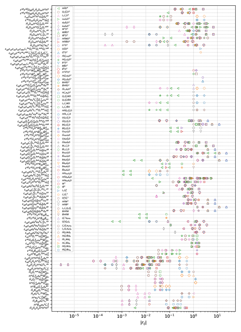
Figure 4: The absolute values of the non-trivial components of $r_{ij}$, defined in (3), for the one generation SM. Each marker is positioned in line with the basis operator corresponding to column $j$, and formatted according to the field composition of the redundant operator corresponding to the leading coefficient in the row $i$. We define the marginal couplings in terms of the measured coefficients of the three generation Standard Model: the Higgs quartic and gauge couplings equal those measured at the $Z$ pole, whereas the Yukawa couplings are set by measurements of the heaviest generation: $y_{u}=\frac{m_{t}}{v}$, $y_{d}=\frac{m_{b}}{v}$, $y_{e}=\frac{m_{\tau}}{v}$.

Appendix A Index conventions

For an $N$ index group

$$\epsilon^{12\cdots N}=-\epsilon_{12\cdots N}=1;\qquad\delta^{a}_{b}=\begin{cases}1&\text{if $a=b$,}\\ 0&\text{otherwise.}\end{cases}$$ (18)

We use the spinor index conventions of Dreiner:2008tw with a mostly-minus metric $\eta_{\mu\nu}=\mathrm{diag}(+1,-1,-1,-1)$ and totally antisymmetric tensor $\epsilon^{0123}=-\epsilon_{0123}=+1$. With the use of the tensors $\sigma^{\mu}_{\alpha\dot{\alpha}}$ and $\bar{\sigma}_{\mu}^{\dot{\alpha}\alpha}$ and relations (2.47-2.53) of Dreiner:2008tw

$$\sigma^{\mu}_{\alpha\dot{\alpha}}\bar{\sigma}_{\mu}^{\dot{\beta}\beta}=2\delta_{\alpha}{}^{\beta}\delta^{\dot{\beta}}{}_{\dot{\alpha}}\,,$$ (19)

$$\sigma^{\mu}_{\alpha\dot{\alpha}}\sigma_{\mu\beta\dot{\beta}}=2\epsilon_{\alpha\beta}\epsilon_{\dot{\alpha}\dot{\beta}}\,,$$ (20)

$$\bar{\sigma}^{\mu\dot{\alpha}\alpha}\bar{\sigma}_{\mu}^{\dot{\beta}\beta}=2\epsilon^{\alpha\beta}\epsilon^{\dot{\alpha}\dot{\beta}}\,,$$ (21)

$${[\sigma^{\mu}\bar{\sigma}^{\nu}+\sigma^{\nu}\bar{\sigma}^{\mu}]_{\alpha}}^{\beta}=2\eta^{\mu\nu}\delta_{\alpha}{}^{\beta}\,,$$ (22)

$$[\bar{\sigma}^{\mu}\sigma^{\nu}+\bar{\sigma}^{\nu}\sigma^{\mu}]^{\dot{\alpha}}{}_{\dot{\beta}}=2\eta^{\mu\nu}\delta^{\dot{\alpha}}{}_{\dot{\beta}}\,,$$ (23)

$$\sigma^{\mu}\bar{\sigma}^{\nu}\sigma^{\rho}=\eta^{\mu\nu}\sigma^{\rho}-\eta^{\mu\rho}\sigma^{\nu}+\eta^{\nu\rho}\sigma^{\mu}+i\epsilon^{\mu\nu\rho\kappa}\sigma_{\kappa}\,,$$ (24)

$$\bar{\sigma}^{\mu}\sigma^{\nu}\bar{\sigma}^{\rho}=\eta^{\mu\nu}\bar{\sigma}^{\rho}-\eta^{\mu\rho}\bar{\sigma}^{\nu}\eta^{\nu\rho}\bar{\sigma}^{\mu}-i\epsilon^{\mu\nu\rho\kappa}\bar{\sigma}_{\kappa}\,,$$ (25)

expressions involving vector and spinor Lorentz indices may be easily converted. For expressions with a single vector index we define

$$A_{\alpha\dot{\alpha}}=\sigma^{\mu}_{\alpha\dot{\alpha}}A_{\mu},\qquad D_{\alpha\dot{\alpha}}=\sigma^{\mu}_{\alpha\dot{\alpha}}D_{\mu},$$ (26)

whence we derive

$$A_{\mu}=\frac{1}{2}\bar{\sigma}_{\mu}^{\dot{\alpha}\alpha}A_{\alpha\dot{\alpha}},\qquad D_{\mu}=\frac{1}{2}\bar{\sigma}_{\mu}^{\dot{\alpha}\alpha}D_{\alpha\dot{\alpha}}.$$ (27)

For expressions with two vector indices, such as a field strength $F_{\mu\nu}$ or its dual $\tilde{F}_{\mu\nu}$, we define

$$F_{\alpha\dot{\alpha}\beta\dot{\beta}}=\sigma^{\mu}_{\alpha\dot{\alpha}}\sigma^{\nu}_{\beta\dot{\beta}}F_{\mu\nu},\qquad\tilde{F}_{\alpha\dot{\alpha}\beta\dot{\beta}}=\sigma^{\mu}_{\alpha\dot{\alpha}}\sigma^{\nu}_{\beta\dot{\beta}}\tilde{F}_{\mu\nu},$$ (28)

such that

$$F_{\mu\nu}=\frac{1}{4}\bar{\sigma}_{\mu}^{\dot{\alpha}\alpha}\bar{\sigma}_{\nu}^{\dot{\beta}\beta}F_{\alpha\dot{\alpha}\beta\dot{\beta}},\qquad\tilde{F}_{\mu\nu}=\frac{1}{4}\bar{\sigma}_{\mu}^{\dot{\alpha}\alpha}\bar{\sigma}_{\nu}^{\dot{\beta}\beta}\tilde{F}_{\alpha\dot{\alpha}\beta\dot{\beta}}\,,$$ (29)

where $F_{\alpha\dot{\alpha}\beta\dot{\beta}}$ and $\tilde{F}_{\alpha\dot{\alpha}\beta\dot{\beta}}$ may be expressed in terms of Lorentz group irreps $F_{\alpha\beta}$ and $\bar{F}_{\dot{\alpha}\dot{\beta}}$:

$$F_{\alpha\dot{\alpha}\beta\dot{\beta}}=-\frac{1}{2}(\epsilon_{\dot{\alpha}\dot{\beta}}F_{\alpha\beta}+\epsilon_{\alpha\beta}\bar{F}_{\dot{\alpha}\dot{\beta}}),\qquad\tilde{F}_{\alpha\dot{\alpha}\beta\dot{\beta}}=-\frac{1}{2}i(\epsilon_{\dot{\alpha}\dot{\beta}}F_{\alpha\beta}-\epsilon_{\alpha\beta}\bar{F}_{\dot{\alpha}\dot{\beta}}).$$ (30)

If $F_{\mu\nu}=\partial_{\mu}A_{\nu}-\partial_{\nu}A_{\mu}$, helpful consequences of the above conventions include

$$F_{\alpha\beta}=\epsilon^{\dot{\alpha}\dot{\beta}}F_{\alpha\dot{\alpha}\beta\dot{\beta}}=\epsilon^{\dot{\alpha}\dot{\beta}}(\partial_{\alpha\dot{\alpha}}A_{\beta\dot{\beta}}-\partial_{\beta\dot{\beta}}A_{\alpha\dot{\alpha}}),$$ (31)

$$\bar{F}_{\dot{\alpha}\dot{\beta}}=\epsilon^{\alpha\beta}F_{\alpha\dot{\alpha}\beta\dot{\beta}}=\epsilon^{\alpha\beta}(\partial_{\alpha\dot{\alpha}}A_{\beta\dot{\beta}}-\partial_{\beta\dot{\beta}}A_{\alpha\dot{\alpha}}).$$ (32)

Note that, alternatively, one can use the tensors

$$(\sigma^{\mu\nu})_{\alpha}^{\beta}=\frac{1}{4}i(\sigma^{\mu}_{\alpha\dot{\alpha}}\bar{\sigma}^{\nu\,\dot{\alpha}\beta}-\sigma^{\nu}_{\alpha\dot{\alpha}}\bar{\sigma}^{\mu\,\dot{\alpha}\beta})$$ (33)

$$(\bar{\sigma}^{\mu\nu})^{\dot{\alpha}}_{\dot{\beta}}=\frac{1}{4}i(\bar{\sigma}^{\mu\,\dot{\alpha}\alpha}\sigma^{\nu}_{\alpha\dot{\beta}}-\bar{\sigma}^{\nu\,\dot{\alpha}\alpha}\sigma^{\mu}_{\alpha\dot{\beta}})$$ (34)

to convert directly between different forms of the field strength:

$$F_{\alpha\beta}=2i(\sigma^{\mu\nu})_{\alpha}^{\gamma}\epsilon_{\gamma\beta}F_{\mu\nu};\qquad\bar{F}_{\dot{\alpha}\dot{\beta}}=2i\epsilon_{\dot{\alpha}\dot{\gamma}}(\bar{\sigma}^{\mu\nu})^{\dot{\gamma}}_{\dot{\beta}}F_{\mu\nu};$$ (35)

$$F^{\mu\nu}-i\tilde{F}^{\mu\nu}=-\frac{1}{2}iF_{\alpha\gamma}\epsilon^{\gamma\beta}(\sigma^{\mu\nu})_{\beta}^{\alpha};\qquad F^{\mu\nu}+i\tilde{F}^{\mu\nu}=-\frac{1}{2}i\epsilon^{\dot{\alpha}\dot{\gamma}}\bar{F}_{\dot{\gamma}\dot{\beta}}(\bar{\sigma}^{\mu\nu})^{\dot{\beta}}_{\dot{\alpha}}\,.$$ (36)

A four component Dirac spinor may be expanded in terms of the components of a left-handed, $L^{\alpha}$, and right-handed, $R^{\dot{\alpha}}$, Weyl spinor, such that

$$\Psi=\begin{pmatrix}L_{\alpha}\\ R^{\dot{\alpha}}\end{pmatrix}={\scriptsize\begin{pmatrix}L_{1}\\ L_{2}\\ R^{1}\\ R^{2}\end{pmatrix}},$$ (37)

and its conjugates are

$$\bar{\Psi}=\begin{pmatrix}\bar{R}^{\alpha}&\bar{L}_{\dot{\alpha}}\end{pmatrix};\qquad\Psi^{C}=\begin{pmatrix}\bar{R}_{\alpha}\\ \bar{L}^{\dot{\alpha}}\end{pmatrix}\,.$$ (38)

Gamma matrices may be similarly expanded as

$$\gamma^{\mu}=\begin{pmatrix}0&\sigma^{\mu}_{\alpha\dot{\beta}}\\ \bar{\sigma}^{\mu\dot{\alpha}\beta}&0\end{pmatrix};\qquad\gamma^{5}=\begin{pmatrix}-\delta_{\alpha}^{\beta}&0\\ 0&\delta^{\dot{\alpha}}_{\dot{\beta}}\end{pmatrix};\qquad\frac{1}{4}i[\gamma^{\mu},\gamma^{\nu}]=\begin{pmatrix}(\sigma^{\mu\nu})_{\alpha}^{\beta}&0\\ 0&(\bar{\sigma}^{\mu\nu})^{\dot{\alpha}}_{\dot{\beta}}\end{pmatrix}\,.$$ (39)

We normalize the non-Abelian vector potentials of the SM such that

$$(W_{\alpha\dot{\alpha}})^{a}_{b}=\frac{1}{2}W_{\alpha\dot{\alpha}}^{i}(\sigma^{i})^{a}_{b};\qquad(G_{\alpha\dot{\alpha}})^{a}_{b}=\frac{1}{2}G_{\alpha\dot{\alpha}}^{i}(\lambda^{i})^{a}_{b}\,,$$ (40)

where $(\lambda^{i})^{a}_{b}$ is the value of the $a$th row and $b$th column of the $i$th Gellmann matrix, and similarly for the Pauli sigma matrices $(\sigma^{i})^{a}_{b}$. $G^{i}$, $i=1,\ldots,8$, and $W^{i}$, $i=1,\ldots,3$, are the canonical gauge fields found in, for instance, the listing of the Warsaw basis Grzadkowski:2010es . With the use of the Fierz relations,

$$(\sigma^{i})^{a}_{b}(\sigma^{i})^{c}_{d} =2\delta^{a}_{d}\delta^{c}_{b}-\delta^{a}_{b}\delta^{c}_{d}$$ (41)

$$(\lambda^{i})^{a}_{b}(\lambda^{i})^{c}_{d} =2\delta^{a}_{d}\delta^{c}_{b}-\frac{2}{3}\delta^{a}_{b}\delta^{c}_{d}$$ (42)

we can deduce the correct normalization of the kinetic terms, e.g.,

$$-\frac{1}{4}W^{i}_{\mu\nu}W^{i\,\mu\nu}=\frac{1}{16}\left((W^{\alpha\beta})^{a}_{b}(W_{\alpha\beta})^{b}_{a}+(\bar{W}^{\dot{\alpha}\dot{\beta}})^{a}_{b}(\bar{W}_{\dot{\alpha}\dot{\beta}})^{b}_{a}\right)\,,$$ (43)

$$-\frac{1}{4}G^{i}_{\mu\nu}G^{i\,\mu\nu}=\frac{1}{16}\left((G^{\alpha\beta})^{a}_{b}(G_{\alpha\beta})^{b}_{a}+(\bar{G}^{\dot{\alpha}\dot{\beta}})^{a}_{b}(\bar{G}_{\dot{\alpha}\dot{\beta}})^{b}_{a}\right)\,.$$ (44)

Appendix B The structure of operator relations in a generic 4d EFT

Following the procedure of Cheung:2015aba , we define two integer coordinates $n$ and $\sum h$ for each monomial EFT operator as, respectively, the number of fields and the sum of the helicities $h$ of the particle created by the action of each field on the vacuum. For fields that are scalar $\phi$, left- and right-handed Weyl fermions $\psi$ and $\bar{\psi}$, and left- and right-handed field strengths $F$ and $\bar{F}$, $h=0,+\frac{1}{2},-\frac{1}{2},+1,-1$ respectively. We enumerate the possible field compositions of dimension 6 operators allowed by Lorentz symmetry and arrange them by their coordinates in Fig. 5 (cf. Fig. 1 of Cheung:2015aba ).

Consider how redundancy relations allow one to move around the table of Fig. 5. IBP and Fierz relations ‘trivially’ mix operators with the same field composition, and therefore with the same coordinates $(n,\sum h)$. The other two kinds can be viewed as expressing a higher derivative operator in terms of an equivalent sum of lower derivative ones.

One, replacing a commutator of derivatives with a field strength generically yields a combination of terms, some with an additional $F$, some with an $\bar{F}$ (one of these may be forbidden by Lorentz symmetry). Thus, starting with an operator with coordinates $(n,\sum h)$, one ends up with operators at $(n+1,\sum h+1)$ and $(n+1,\sum h-1)$.

Two, replacing the free part of an EOM with the interacting parts amounts to, diagrammatically, taking a graph comprising just an insertion of a higher derivative dim 6 operator, and adding a dim 4 vertex to one of the legs on which the derivative(s) act(s) (see Figure 3.5). This composite, two vertex graph may have the same leading order momentum piece as a simple insertion of a lower derivative dim 6 operator, when the external legs are on shell. We may assume the fields are massless, as relevant interactions do not affect the EOM relations. Thus, by (12) of Cheung:2015aba , the coordinates $(n_{i},(\sum h)_{i})$ of such a composite amplitude (and by extension the weights of the corresponding lower derivative operator) are related to the weights of the constituent vertices $(n_{j},(\sum h)_{j})$ and $(n_{k},(\sum h)_{k})$ by:

$$n_{i}=n_{j}+n_{k}-2;\qquad(\sum h)_{i}=(\sum h)_{j}+(\sum h)_{k}.$$ (45)

The weights of possible dim 4 vertices are as follows. A gauge or Yukawa coupling is $(n,\sum h)=(3,\pm 1)$. Anything proportional to a scalar quartic is $(4,0)$. Therefore, the part of an EOM relation proportional to a gauge or Yukawa coupling lies one unit right and one unit either up or down in the table of operators, relative to the original higher derivative operator. For the part proportional to a Higgs quartic, it lies two units to the right.

Figure 5: A schematic ‘map’ of all dimension 6 operators allowed by Lorentz symmetry, cut in half about its axis of symmetry $\sum h=0$ (reflected in this line are the hermitian conjugates of the operators shown). Arrows show the movement induced by equation of motion relations and commutation of derivative relations in the space of dim 6 operators, colour-coded to show $\phi$ EOMs (blue), $\psi$ EOMs (green, short dashed), $F$ EOMs (red, long dashed), and replacing derivatives with field strengths (grey, dash-dotted).

Figure 5 allows us to understand two examples of dimension 6 monomial operators in the SM, which are not related to any others. One, an $H^{2}G^{2}$ (class $F^{2}\phi^{2}$) operator could only be reached from an operator of class $F\phi D^{2}$. However, all such $GHD^{2}$ operators are forbidden by gauge symmetries. Two, baryon violating operators of the form $\psi^{4}$, $\psi^{2}\bar{\psi}^{2}$, and $\bar{\psi}^{4}$, are only reachable from operators of class $F\psi\bar{\psi}D$ and $\psi^{2}D^{2}$, as well as their conjugates. The baryon violating operators contain three quarks, and all relations preserve the parity of the number of quarks. However, there are no gauge invariant operators of the form $F\psi\bar{\psi}D$ or $\psi^{2}D^{2}$ containing a single quark, leaving the baryon violating four fermion operators unrelated to both baryon conserving operators, and also unrelated to each other.

References

- (1) M. B. Einhorn and J. Wudka, The Bases of Effective Field Theories, Nucl.Phys. B876 (2013) 556–574, [1307.0478].
- (2) B. Gripaios and D. Sutherland, An operator basis for the Standard Model with an added scalar singlet, JHEP 08 (2016) 103, [1604.07365].
- (3) W. Buchmuller and D. Wyler, Effective Lagrangian Analysis of New Interactions and Flavor Conservation, Nucl. Phys. B268 (1986) 621–653.
- (4) B. Grzadkowski, M. Iskrzynski, M. Misiak and J. Rosiek, Dimension-Six Terms in the Standard Model Lagrangian, JHEP 10 (2010) 085, [1008.4884].
- (5) A. Falkowski, B. Fuks, K. Mawatari, K. Mimasu, F. Riva and V. Sanz, Rosetta: an operator basis translator for Standard Model effective field theory, Eur. Phys. J. C75 (2015) 583, [1508.05895].
- (6) A. Falkowski, Higgs Basis: Proposal for an EFT basis choice for LHC HXSWG, .
- (7) L. Lehman and A. Martin, Hilbert Series for Constructing Lagrangians: expanding the phenomenologist’s toolbox, Phys. Rev. D91 (2015) 105014, [1503.07537].
- (8) B. Henning, X. Lu, T. Melia and H. Murayama, Hilbert series and operator bases with derivatives in effective field theories, 1507.07240.
- (9) L. Lehman and A. Martin, Low-derivative operators of the Standard Model effective field theory via Hilbert series methods, JHEP 02 (2016) 081, [1510.00372].
- (10) B. Henning, X. Lu, T. Melia and H. Murayama, 2, 84, 30, 993, 560, 15456, 11962, 261485, …: Higher dimension operators in the SM EFT, JHEP 08 (2017) 016, [1512.03433].
- (11) B. Henning, X. Lu, T. Melia and H. Murayama, Operator bases, -matrices, and their partition functions, JHEP 10 (2017) 199, [1706.08520].
- (12) J. C. Criado, MatchingTools: a Python library for symbolic effective field theory calculations, Comput. Phys. Commun. 227 (2018) 42–50, [1710.06445].
- (13) C. Arzt, Reduced effective Lagrangians, Phys. Lett. B342 (1995) 189–195, [hep-ph/9304230].
- (14) A. Meurer, C. P. Smith, M. Paprocki, O. Čertík, S. B. Kirpichev, M. Rocklin et al., Sympy: symbolic computing in python, PeerJ Computer Science 3 (Jan., 2017) e103.
- (15) H. K. Dreiner, H. E. Haber and S. P. Martin, Two-component spinor techniques and Feynman rules for quantum field theory and supersymmetry, Phys. Rept. 494 (2010) 1–196, [0812.1594].
- (16) C. Cheung and C.-H. Shen, Nonrenormalization Theorems without Supersymmetry, Phys. Rev. Lett. 115 (2015) 071601, [1505.01844].