The Carnegie RR Lyrae Program: Mid-infrared Period-Luminosity relations of RR Lyrae stars in Reticulum

Abstract

We analysed 30 RR Lyrae stars (RRLs) located in the Large Magellanic Cloud (LMC) globular cluster Reticulum that were observed in the 3.6 and 4.5 $\mu m$ passbands with the Infrared Array Camera (IRAC) on board of the Spitzer Space Telescope. We derived new mid-infrared (MIR) period-luminosity ($PL$) relations. The zero points of the $PL$ relations were estimated using the trigonometric parallaxes of five bright Milky Way (MW) RRLs measured with the Hubble Space Telescope (HST) and, as an alternative, we used the trigonometric parallaxes published in the first Gaia data release (DR1) which were obtained as part of the Tycho-Gaia Astrometric Solution (TGAS) and the parallaxes of the same stars released with the second Gaia data release (DR2). We determined the distance to Reticulum using our new MIR $PL$ relations and found that distances calibrated on the TGAS and DR2 parallaxes are in a good agreement and, generally, smaller than distances based on the HST parallaxes, although they are still consistent within the respective errors. We conclude that Reticulum is located $\sim 3$  kpc closer to us than the barycentre of the LMC.

1 Introduction

Knowledge of the distances to celestial objects is crucially important to all branches of astronomy. In order to estimate distances, astronomers have developed a number of different techniques. Some methods, such as the trigonometric parallax, are based on geometric principles, while others invoke the use of primary distance indicators such as Cepheids or RR Lyrae (RRL) variables, which in turn are calibrated using the geometric methods. RRL stars (RRLs) are radially pulsating variables which are abundant in globular clusters (GCs) and in the halos of galaxies. The RRLs are old ($>10$ Gyr), low-mass ($\sim 0.6-0.8$ $M_{\odot}$) core-helium burning stars that lie within the instability strip crossing the horizontal branch (HB) of the colour-magnitude diagram (CMD). They are divided into those pulsating in the fundamental (RRab) and first-overtone (RRc) modes, and both modes simultaneously (RRd). RRLs are an excellent tool to estimate distances in the Milky Way (MW) and to Local Group galaxies because they conform to an optical luminosity-metallicity ($M_{V}-{\rm[Fe/H]}$) relation and to infrared period-luminosity ($PL$) and $PL$-metallicity ($PLZ$) relations. The near-infrared (NIR) and mid-infrared (MIR) $PL$ relations of RRLs have several advantages in comparison with the visual $M_{V}-{\rm[Fe/H]}$ relation; specifically, a milder dependence of the luminosity on metallicity and lower sensitivity to interstellar extinction. Indeed, extinction in the 3.6 and 4.5 $\mu m$ bands is much reduced with respect to the visual passband ($A_{3.6}\sim 0.06A_{V}$ and $A_{4.5}\sim 0.05A_{V}$, Monson et al. 2012). Furthermore, the intrinsic scatter of the RRL (and Cepheid) $PL$ relations decreases with increasing the wavelength (Madore & Freedman, 2012) and the MIR light curves of RRLs (and Cepheids) have smaller amplitudes than in the optical passbands, hence, the determination of the mean magnitudes is easier and more precise. Moreover, a number of studies also indicate that the $M_{V}-{\rm[Fe/H]}$ relation may be not linear (Caputo et al. 2000; Rey et al. 2000; Bono et al. 2003), which is not the case for the MIR $PL$ relations.

In order to study the RRL $PL$ relation in the MIR passbands it is necessary to have a statistically significant sample of variables with firmly established classification, well-known periods and accurately determined mean MIR magnitudes. In particular, for the present study of the MIR RRL $PL$ relation we selected Reticulum, an old GC located in the Large Magellanic Cloud (LMC), $\sim$ 11 degrees away from the centre of its host galaxy (Demers & Kunkel, 1976). The RRL population of Reticulum has been studied by several authors. Demers & Kunkel (1976) discovered 22 RRLs in the cluster. Walker (1992) later identified 10 additional RRLs bringing the total number of RRLs in Reticulum to 32 (22 RRab, 9 RRc and 1 candidate RRd star). Ripepi et al. (2004) combined Walker (1992)’s photometry with their observations in the B and V passbands and detected double-mode behaviour in four of the previously discovered RRL variables.

NIR $K$-band light curves with approximately 12 phase points per source were published by Dall’Ora et al. (2004) for 30 of the RRLs in Reticulum. Mean $K$-band magnitudes were estimated by fitting the light curves with templates from Jones et al. (1996) and then used to build a NIR $K$-band $PL$ relation.

Most recently, in their optical study of Reticulum, Kuehn et al. (2013) identified a secondary pulsation mode in two RRLs changing their classifications from RRc to RRd. Hence, the RRLs in Reticulum now list 22 RRab, 4 RRc and 6 RRd stars. Kuehn et al. (2013) estimated an accuracy of $10^{-5}$ days for the periods of the RRab and RRc variables and an uncertainty approximately one order of magnitude larger for the periods of the RRd stars.

All RRLs in the cluster share the same reddening, distance and metallicity (Kuehn et al., 2013). Additionally, the majority of the RRLs in the cluster are located in uncrowded fields, which allows us to accurately determine their mean magnitudes in the 3.6 and 4.5 $\mu m$ passbands.

In this paper we present the first MIR $PL$ relations defined using RRLs in a system outside our Galaxy, and compare them with empirical studies of the MIR $PL$ relation based on field and GC MW RRLs (Madore et al. 2013, Dambis et al. 2014, Klein et al. 2014, Neeley et al. 2015, Gaia Collaboration et al. 2017).

This study is part of the Carnegie RR Lyrae Program (CRRP, PI Freedman). CRRP is a Warm Spitzer Cycle 9 Exploration Science program which uses the [3.6] and [4.5] channels of the Infrared Array Camera (IRAC, Fazio et al. 2004) to study MW RRL. In addition to the Reticulum observations described here, CRRP is also studying $\sim 30$ GCs in the MW and LMC, a sample of field RRLs in the MW (Monson et al., 2017), and a large number of bulge RRLs. CRRP is complementary program to the Spitzer Merger History and Shape of the Halo Program (SMHASH, PI Johnston), which uses halo, stream, GC, and dwarf spheroidal galaxy (dSph) RRLs to examine the MW’s structure (e.g. Neeley et al. 2017, Hendel et al. 2018, Garofalo et al. 2018).

To calibrate the zero point of our MIR $PL$ relations we used trigonometric parallaxes of five Galactic RRLs measured with the Fine Guide Sensor (FGS) on board of the Hubble Space Telescope (HST) by Benedict et al. (2011). As a comparison, we have also derived the zero points for our MIR $PL$ relations using the trigonometric parallaxes for these same stars from the first data release (DR1) of the European Space Agency (ESA) mission Gaia (Gaia Collaboration et al. 2016a, Gaia Collaboration et al. 2016b), that were computed as part of the Tycho-Gaia Astrometric Solution (TGAS, Lindegren et al. 2016), in addition to the most recent Gaia parallaxes released with the second Data Release (DR2, Gaia Collaboration et al. 2018; Lindegren et al. 2018).

The paper is organised as follows. In Section 2, we describe the observations and data reduction, and provide MIR mean magnitudes and amplitudes of the 30 RRLs in Reticulum that form the basis of the present study. In Section 3 we present the results of fitting the RRL $PL$ relations in the 3.6 and 4.5 $\mu m$ passbands and describe the calibration of their zero points. We also present a comparison of our $PL$ relations with those in the literature. In Section 4 we use our new relations to estimate the distance to Reticulum. A summary of our results is provided in Section 5.

2 Data

2.1 Observations and data reduction

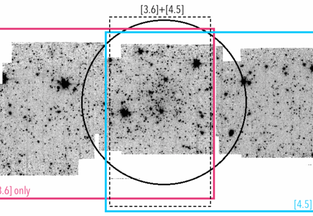
Figure 1: Coverage of the 3.6 $\mu m$ (magenta box) and 4.5 $\mu m$ (cyan box) images of Reticulum. The cluster is located at the intersection of the two fields of view (black dashed line). The black circle shows the location of the cluster, and has a radius equal to two half-light radii of Reticulum (2.35 arcmin, Bica et al. 1999).

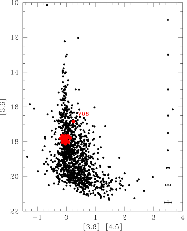
Figure 2: CMD ([3.6] vs [3.6]$-$[4.5]) of 1284 sources in the field of Reticulum observed with Spitzer in both 3.6 and 4.5 $\mu m$ passbands. RRLs are marked in red. Typical uncertainties of the photometry per magnitude bin estimated with ALLFRAME are shown on the right.

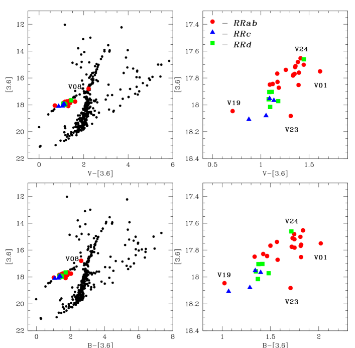
Figure 3: Left panels: CMDs ([3.6] vs $V-$ [3.6] and [3.6] vs $B-$ [3.6], in the upper- and bottom-left panels, respectively) of 364 sources in the field of the Reticulum cluster that we observed with Spitzer. $B$ and $V$ photometry for these objects is available from Jeon et al. (2014). Red circles, blue triangles and green squares represent RRab, RRc and RRd stars, respectively. Right panels: Zoom-in of the region populated by RRLs in the CMDs shown in the left panels. For clarity reasons we do not plot the RRL V08 in the right panels of the figure.

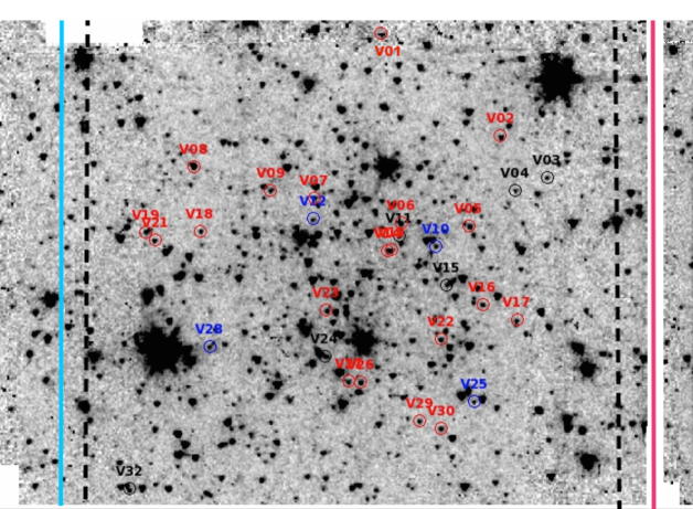
Figure 4: Zoom-in of Fig. 1 showing the region of the Reticulum cluster. Open red, blue and black circles indicate the Reticulum RRab, RRc and RRd stars, respectively.

The Spitzer Space Telescope (Werner et al., 2004) was launched on 2003 August 25 with the main goal of providing a unique, infrared view of the universe. It operates at wavelengths which have low sensitivity to extinction and it has proven to be a perfect tool for undertaking variable star studies (Freedman et al., 2011) as it was able to be scheduled so as to uniformly sample the light curves of variable stars providing high-precision stellar photometry that is very stable in its calibrated zero point.

Reticulum was observed during Cycle 9 of the Warm Spitzer mission. The observations were executed on 2012 November 27 and consist of 12 epochs (each with individual exposures of $\sim 31$ s), simultaneously in the 3.6 and 4.5 $\mu m$ passbands. The observations were distributed over a time interval of approximately 14 hours, corresponding to the longest period RRL in the field.

This spacing and time coverage were chosen to optimise the phase coverage of the RRLs that were known to exist in the field. The total area mapped by the Spitzer observations of Reticulum is shown in Figure 1. The cluster is located at the intersection of the Spitzer [3.6] and [4.5] fields of view. The elongated field shape is owing to the dither pattern of the observations. While “on target" observations are taken in one IRAC band, adjacent “off target” observations are taken simultaneously in the other passband. Colour information is available for the central region, and single band data are available for the two side regions. We outlined the cluster with a black circle of radius equal to two half-light radii of Reticulum (2.35 arcmin, Bica et al. 1999).

Table 1: Main properties of the 364 sources in common between our MIR catalogues and the visual catalogues of Jeon et al. (2014)

ID Jeona	ID Kuehnb	RA	Dec	Flagc	B	V	[3.6]d	[4.5]d
		(J2000)	(J2000)		(mag)	(mag)	(mag)	(mag)
Reticulum 225	V01	04:35:51.5	$-$58:51:03.4	1	19.771 $\pm$ 0.115	19.364 $\pm$ 0.084	17.751	17.826
Reticulum 279	V02	04:35:56.6	$-$58:52:32.1	1	19.467 $\pm$ 0.256	19.074 $\pm$ 0.205	17.717	17.678
Reticulum 269	V03	04:35:58.6	$-$58:53:06.7	1	19.385 $\pm$ 0.216	19.112 $\pm$ 0.163	17.997	17.932
Reticulum 272	V04	04:36:00.3	$-$58:52:50.0	1	19.307 $\pm$ 0.218	19.040 $\pm$ 0.178	17.963	17.974
Reticulum 250	V05	04:36:04.1	$-$58:52:29.3	1	19.440 $\pm$ 0.286	19.070 $\pm$ 0.239	17.669	17.611
Reticulum 294	V06	04:36:05.4	$-$58:51:47.8	1	19.495 $\pm$ 0.257	19.112 $\pm$ 0.216	17.747	17.826
Reticulum 220	V07	04:36:05.5	$-$58:50:51.8	1	19.185 $\pm$ 0.504	18.943 $\pm$ 0.421	17.821	17.978
Reticulum 288	V08	04:36:05.7	$-$58:49:34.3	1	19.421 $\pm$ 0.189	19.016 $\pm$ 0.129	16.841	16.602
Reticulum 237	V09	04:36:05.9	$-$58:50:24.5	1	19.306 $\pm$ 0.341	18.998 $\pm$ 0.286	17.726	17.756
Reticulum 273	V10	04:36:06.4	$-$58:52:12.6	1	19.365 $\pm$ 0.224	19.102 $\pm$ 0.200	17.960	18.002
Reticulum 259	V11	04:36:06.4	$-$58:51:48.7	1	19.280 $\pm$ 0.268	18.992 $\pm$ 0.228	17.913	18.037
Reticulum 243	V12	04:36:07.1	$-$58:50:54.9	1	19.175 $\pm$ 0.105	18.984 $\pm$ 0.084	18.124	18.157
Reticulum 255	V13	04:36:07.8	$-$58:51:46.8	1	19.531 $\pm$ 0.322	19.116 $\pm$ 0.255	17.773	17.743
Reticulum 244	V14	04:36:07.8	$-$58:51:44.4	1	19.427 $\pm$ 0.324	19.065 $\pm$ 0.246	17.683	17.792
Reticulum 262	V15	04:36:09.1	$-$58:52:25.8	1	19.453 $\pm$ 0.162	19.152 $\pm$ 0.142	17.980	18.050
Reticulum 233	V16	04:36:09.8	$-$58:52:50.7	1	19.254 $\pm$ 0.436	19.002 $\pm$ 0.340	17.814	17.823
Reticulum 298	V17	04:36:10.3	$-$58:53:13.6	1	19.267 $\pm$ 0.419	18.937 $\pm$ 0.313	17.754	17.850
Reticulum 261	V18	04:36:10.6	$-$58:49:50.2	1	19.511 $\pm$ 0.308	19.145 $\pm$ 0.263	17.733	17.760
Reticulum 227	V19	04:36:11.9	$-$58:49:18.1	1	19.070 $\pm$ 0.449	18.754 $\pm$ 0.332	18.029	17.952
Reticulum 287	V21	04:36:12.3	$-$58:49:24.3	1	19.578 $\pm$ 0.283	19.155 $\pm$ 0.217	17.798	17.663
Reticulum 276	V22	04:36:13.4	$-$58:52:32.0	1	19.309 $\pm$ 0.363	18.967 $\pm$ 0.260	17.801	17.989
Reticulum 258	V23	04:36:13.8	$-$58:51:19.0	1	19.790 $\pm$ 0.134	19.392 $\pm$ 0.120	18.034	18.170
Reticulum 248	V24	04:36:17.3	$-$58:51:26.6	1	19.377 $\pm$ 0.273	19.106 $\pm$ 0.229	17.660	17.803
Reticulum 277	V25	04:36:17.4	$-$58:53:02.6	1	19.367 $\pm$ 0.255	19.134 $\pm$ 0.178	18.058	18.097
Reticulum 296	V26	04:36:18.5	$-$58:51:51.8	1	19.490 $\pm$ 0.155	19.065 $\pm$ 0.113	17.668	17.698
Reticulum 295	V27	04:36:18.7	$-$58:51:44.3	1	19.669 $\pm$ 0.263	19.243 $\pm$ 0.200	17.779	17.837
Reticulum 246	V28	04:36:19.2	$-$58:50:15.5	1	19.294 $\pm$ 0.223	19.043 $\pm$ 0.166	18.003	18.071
Reticulum 223	V29	04:36:20.1	$-$58:52:33.5	1	19.446 $\pm$ 0.381	19.058 $\pm$ 0.285	17.832	17.847
Reticulum 236	V30	04:36:20.2	$-$58:52:47.7	1	19.582 $\pm$ 0.268	19.119 $\pm$ 0.284	17.837	17.835
Reticulum 268	V32	04:36:32.0	$-$58:49:53.2	1	19.319 $\pm$ 0.207	19.016 $\pm$ 0.160	17.953	18.003
Reticulum 5	$-$	04:35:52.8	$-$58:49:40.5	0	13.825 $\pm$ 0.017	13.191 $\pm$ 0.020	12.034	11.625
Reticulum 12	$-$	04:35:50.9	$-$58:52:55.7	0	15.661 $\pm$ 0.014	14.151 $\pm$ 0.014	10.144	10.805
Reticulum 19	$-$	04:36:19.4	$-$58:54:20.6	0	15.950 $\pm$ 0.006	15.081 $\pm$ 0.016	13.103	13.121
Reticulum 23	$-$	04:36:12.3	$-$58:54:04.4	0	16.149 $\pm$ 0.009	15.294 $\pm$ 0.017	12.992	12.977
Reticulum 26	$-$	04:36:22.5	$-$58:49:08.2	0	16.212 $\pm$ 0.008	15.541 $\pm$ 0.016	13.787	13.880

^a Identification from Jeon et al. (2014).

^b Identification from Kuehn et al. (2013).

^c A “1" flag indicates objects from Jeon et al. (2014) that are classified as RRLs by Kuehn et al. (2013), while a “0" flag indicates stars that do not have a counterpart in the Kuehn et al. (2013) catalogue of RRLs.

^d Mean magnitudes in the Spitzer passbands obtained as a result of the data reduction procedure; uncertainties in magnitudes are not provided, since ALLFRAME is known to provide underestimated uncertainties.

This table is published in its entirety at the CDS; a portion is shown here for guidance with respect to its form and content.

For each epoch a single epoch mosaic image was created from the individual basic calibrated data (BCD) frames provided by the Spitzer Science Center, using MOPEX (Makovoz & Khan, 2005). Mosaicked location-correction images for each epoch were also created. Point-spread function (PSF) photometry of the mosaicked images was performed using the DAOPHOT-ALLSTAR-ALLFRAME packages (Stetson 1987, 1994). Firstly, each image mosaic was converted from $MJy/sr$ to counts (DN) using the conversion factor $(MJy/sr$ per $DN/sec)$ and the exposure time provided in the image header. On each epoch the PSF model was created selecting $\sim$ 50 stars uniformly distributed across the frames ( with 30% of stars in common among all epochs). Reticulum has an uncrowded nature, our PSF stars are bright ($m_{[3.6]}<16.741$ mag and $m_{[4.5]}<16.519$ mag) and well isolated. With the ALLSTAR algorithm we fitted the PSF model given by the PSF stars to the sources in each frame. The ALLFRAME routine was then used to perform the PSF photometry simultaneously on images at all epochs. The ALLFRAME catalogue provides instrumental magnitudes for each star in the images with an arbitrary zero point value.

To transform the photometry to standard IRAC Vega magnitudes we selected 53 stars in the 3.6 $\mu m$ and 55 stars in the 4.5 $\mu m$ images, homogeneously distributed over the frames. We obtained aperture photometry of these stars, calibrated to the zero point magnitude (zmag) provided in the IRAC handbook which was then compared with the DAOPHOT instrumental magnitudes in order to derive the final calibrated magnitudes. Point source photometry requires additional array location-dependent photometric corrections. These corrections improve the photometric accuracy for IRAC data by taking into account scattering and distortions, but above all, variations in the effective central wavelengths of the IRAC filters, which depend on the angle of incidence. The final photometric catalogues contain 4068 and 3379 sources in 3.6 and 4.5 $\mu m$, respectively. The 3.6 $\mu m$ photometry spans the range from 21.57 to 9.23 mag, while the 4.5 $\mu m$ photometry ranges from 21.11 to 10.36 mag, where upper limits are owing to saturation. Uncertainties in the 3.6 $\mu m$ magnitudes range from 0.003 to 0.100 mag, while uncertainties in the 4.5 $\mu m$ magnitudes span the range from 0.005 to 0.100 mag. The typical uncertainties at the level of the Reticulum HB ($\sim 18$ mag) are 0.017 mag and 0.022 mag in the 3.6 $\mu m$ and 4.5 $\mu m$ bands, respectively. Typical uncertainties of the photometry per magnitude bin are shown in Fig. 2. We remind the reader that the uncertainties in magnitudes calculated as part of the data reduction procedure using ALLFRAME software can be significantly underestimated.

We used DAOMASTER and DAOMATCH to combine the 3.6 $\mu m$ and 4.5 $\mu m$ catalogues and obtained a list of 1284 sources for which photometry is available in both passbands. The [3.6] vs $([3.6]-[4.5])$ CMD of these sources is shown in Fig. 2, where red dots represent the RRLs. The MIR CMD has its limitations owing to low sensitivity of the luminosity in the MIR passbands to the temperature. Although the HB is not very well distinguished from the Red Giant Branch (RGB) in these passbands, the RRLs in Fig. 2 tracing a well-defined population, both in colour and magnitude allow us to clearly identify the location of the cluster HB.

Jeon et al. (2014) provide $B$, $V$ photometry for 766 sources in Reticulum. We crossmatched the catalogue of Jeon et al. (2014) with our MIR catalogue of 1284 sources and found 364 objects in common. Information on these sources with the apparent $B$ and $V$ magnitudes provided by Jeon et al. (2014) and MIR magnitudes obtained here is presented in Table 1. The [3.6], $(V-[3.6])$ and [3.6], $(B-[3.6])$ CMDs of these 364 sources are shown in the left panels of Fig. 3. The cluster RGB and the HB are well defined, demonstrating the quality of our photometry and the accuracy of the calibration procedure.

2.2 RRLs in Reticulum

Table 2: Identification and properties of the 30 RRLs in Reticulum for which we analysed the Spitzer 3.6 and 4.5 $\mu m$ time-series data.

ID	RA	DEC	Type	P	Log(P)	Epocha	[3.6]b	${\rm Amp_{[3.6]}}$	[4.5]b	${\rm Amp_{[4.5]}}$	$\varpi$	Flagc
	(J2000)	(J2000)		(days)		(HJD)	(mag)	(mag)	(mag)	(mag)	(mas)
V01	04:35:51.5	$-$58:51:03.4	RRab	0.50993	$-$0.29249	56258.032	$17.750\pm 0.109$	0.410	$17.825\pm 0.185$	0.217	$-0.18\pm 0.19$	1
V02	04:35:56.6	$-$58:52:32.1	RRab	0.61869	$-$0.20853	56257.239	$17.719\pm 0.047$	0.153	$17.603\pm 0.108$	0.238	$0.13\pm 0.18$	0
V03	04:35:58.6	$-$58:53:06.7	RRd	0.35350	$-$0.45161	56257.592	$18.015\pm 0.068$	0.204	$17.918\pm 0.077$	0.244	$-0.02\pm 0.18$	0
V04	04:36:00.3	$-$58:52:50.0	RRd	0.35320	$-$0.45198	56268.034	$17.958\pm 0.056$	$-$	$17.908\pm 0.103$	$-$	$0.20\pm 0.18$	0
V05	04:36:04.1	$-$58:52:29.3	RRab	0.57185	$-$0.24272	56257.444	$17.711\pm 0.042$	0.249	$17.617\pm 0.063$	0.322	$0.14\pm 0.21$	0
V06-BL	04:36:05.4	$-$58:51:47.8	RRab	0.59526	$-$0.22529	56257.439	$17.775\pm 0.041$	0.276	$17.862\pm 0.094$	0.363	$-0.01\pm 0.18$	0
V07	04:36:05.5	$-$58:50:51.8	RRab	0.51044	$-$0.29206	56257.550	$17.849\pm 0.052$	0.280	$18.010\pm 0.097$	0.255	$0.43\pm 0.23$	0
V08	04:36:05.7	$-$58:49:34.3	RRab	0.64496	$-$0.19047	56257.608	$16.796\pm 0.055$	0.144	$16.558\pm 0.097$	$-$	$0.19\pm 0.20$	1
V09	04:36:05.9	$-$58:50:24.5	RRab	0.54496	$-$0.26364	56257.824	$17.739\pm 0.047$	0.166	$17.732\pm 0.069$	0.261	$-0.09\pm 0.17$	0
V10	04:36:06.4	$-$58:52:12.6	RRc	0.35256	$-$0.45277	56257.813	$17.967\pm 0.044$	0.185	$17.964\pm 0.077$	0.166	$0.02\pm 0.18$	0
V11	04:36:06.4	$-$58:51:48.7	RRd	0.35540	$-$0.44928	56257.987	$17.904\pm 0.045$	0.160	$18.000\pm 0.103$	0.160	$0.02\pm 0.21$	0
V12	04:36:07.1	$-$58:50:54.9	RRc	0.29627	$-$0.52831	56258.029	$18.108\pm 0.056$	$-$	$18.184\pm 0.104$	$-$	$0.11\pm 0.19$	0
V13	04:36:07.8	$-$58:51:46.8	RRab	0.60958	$-$0.21497	56257.456	$17.782\pm 0.039$	0.175	$17.716\pm 0.055$	0.209	$-0.05\pm 0.18$	0
V14-BL	04:36:07.8	$-$58:51:44.4	RRab	0.58661	$-$0.23165	56257.679	$17.681\pm 0.044$	0.288	$17.728\pm 0.052$	0.289	$0.10\pm 0.19$	0
V15	04:36:09.1	$-$58:52:25.8	RRd	0.35430	$-$0.45063	56257.790	$17.972\pm 0.053$	0.138	$18.040\pm 0.115$	0.200	$-0.04\pm 0.20$	0
V16	04:36:09.8	$-$58:52:50.7	RRab	0.52290	$-$0.28158	56257.913	$17.829\pm 0.056$	0.246	$17.827\pm 0.073$	0.210	$0.10\pm 0.19$	0
V17	04:36:10.3	$-$58:53:13.6	RRab	0.51241	$-$0.29038	56257.599	$17.767\pm 0.045$	0.302	$17.757\pm 0.076$	0.340	$0.39\pm 0.20$	0
V18	04:36:10.6	$-$58:49:50.2	RRab	0.56005	$-$0.25177	56257.751	$17.701\pm 0.050$	0.291	$17.722\pm 0.066$	0.247	$-0.50\pm 0.19$	0
V19	04:36:11.9	$-$58:49:18.1	RRab	0.48485	$-$0.31439	56257.635	$18.046\pm 0.074$	0.360	$17.981\pm 0.155$	0.603	$0.30\pm 0.20$	1
V21	04:36:12.3	$-$58:49:24.3	RRab	0.60700	$-$0.21681	56257.933	$17.760\pm 0.065$	0.292	$17.665\pm 0.089$	0.263	$-0.05\pm 0.20$	0
V22	04:36:13.4	$-$58:52:32.0	RRab	0.51359	$-$0.28938	56257.851	$17.844\pm 0.072$	0.291	$17.880\pm 0.077$	0.351	$-0.35\pm 0.22$	0
V23-BL	04:36:13.8	$-$58:51:19.0	RRab	0.46863	$-$0.32917	56258.153	$18.082\pm 0.070$	0.244	$18.245\pm 0.114$	0.366	$-0.01\pm 0.21$	0/1
V24	04:36:17.3	$-$58:51:26.6	RRd	0.34750	$-$0.45905	56257.864	$17.661\pm 0.067$	0.089	$17.780\pm 0.119$	$-$	$-0.12\pm 0.19$	1
V25	04:36:17.4	$-$58:53:02.6	RRc	0.32991	$-$0.48160	56258.020	$18.080\pm 0.065$	0.191	$18.073\pm 0.077$	0.242	$0.11\pm 0.19$	0
V26	04:36:18.5	$-$58:51:51.8	RRab	0.65696	$-$0.18246	56257.940	$17.653\pm 0.042$	0.100	$17.720\pm 0.087$	0.222	$-0.11\pm 0.19$	0
V27	04:36:18.7	$-$58:51:44.3	RRab	0.51382	$-$0.28919	56257.982	$17.852\pm 0.052$	0.350	$17.900\pm 0.071$	0.331	$-0.31\pm 0.22$	0
V28	04:36:19.2	$-$58:50:15.5	RRc	0.31994	$-$0.49493	56257.701	$17.952\pm 0.065$	0.163	$18.056\pm 0.141$	$-$	$0.23\pm 0.22$	1
V29	04:36:20.1	$-$58:52:33.5	RRab	0.50815	$-$0.29401	56257.682	$17.872\pm 0.067$	0.348	$17.818\pm 0.078$	0.440	$-0.14\pm 0.20$	0
V30	04:36:20.2	$-$58:52:47.7	RRab	0.53501	$-$0.27164	56257.725	$17.769\pm 0.047$	0.242	$17.750\pm 0.076$	0.301	$-0.19\pm 0.18$	0
V32	04:36:32.0	$-$58:49:53.2	RRd	0.35230	$-$0.45309	56257.750	$17.903\pm 0.060$	0.060	$18.083\pm 0.208$	$-$	$0.07\pm 0.22$	1

^a Epoch of maximum light (HJD-2400000) of the 3.6 $\mu m$ light curve. The epoch of maximum light is the same in the 3.6 $\mu m$ and 4.5 $\mu m$ passbands for all sources except for V10. The 4.5 $\mu m$ data of this star had to be shifted by 0.4 in phase.
^b Magnitudes in the Spitzer passbands obtained by fitting a model to the data with the GRATIS software.
^c A “0" in column 13 flags objects which were used to fit the $PL$ relations whereas a “1" flags stars that were discarded. A “0/1" flags V23 because the star was used to fit the the 3.6 $\mu m$ $PL$ relation, but was automatically rejected by the 3-sigma clipping procedure when fitting the 4.5 $\mu m$ $PL$ relation. See text for details.

In this paper we study the MIR (3.6 and 4.5 $\mu m$) time-series photometry of the Reticulum RRLs. We cross-matched our catalogue of 1284 sources with 3.6 and 4.5 $\mu m$ photometry (see Section 2.1) against 32 RRLs from Kuehn et al. (2013) catalogue. Thirty RRLs from the Kuehn et al. sample were identified, while we were not able to find the counterparts of V20 and V31 in our catalogue since these objects belong to non-resolved elongated groups of sources in our data. The 30 RRLs (20 RRab, 4 RRc and 6 RRd stars) are listed in Table 2 adopting the identification number, coordinates, period, and classification in type of Kuehn et al. (2013). Periods range from 0.29627 to 0.65696 days. For the 6 RRd stars we list only the first-overtone periodicity. The positions of the 30 RRLs in the Spitzer images is shown in Fig. 4 with the RRab, RRc and RRd stars marked by red, blue and black open circles, respectively. The 3.6 and 4.5 $\mu m$ light curves are presented in Fig. 5.

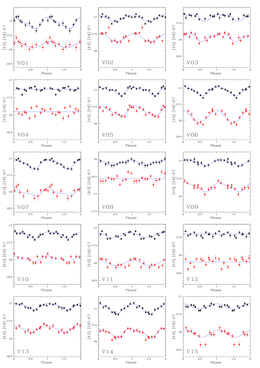
Figure 5: Spitzer MIR light curves of the RRLs in Reticulum analysed in the present study. Black and red dots represent the 3.6 $\mu m$ and 4.5 $\mu m$ data points, respectively, with the 3.6 $\mu m$ shifted by $-0.7$ mag, for clarity. Blue solid lines show the best fit models. Only data points used in the model fitting are shown.

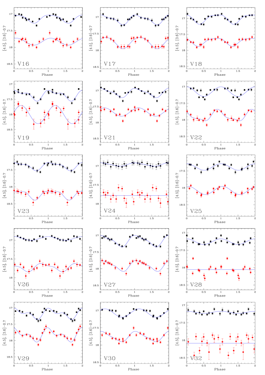
Figure 6: continued

The epoch of maximum light (Column 7 in Table 2) is the same for the 3.6 and 4.5 $\mu m$ passbands for all sources except for V10. The 4.5 $\mu m$ data points of this star had to be shifted by $\sim$ 0.4 in phase when folded according to the epoch in the 3.6 $\mu m$ passband. For a large majority of the RRLs we determined mean 3.6 and 4.5 $\mu m$ magnitudes by Fourier fitting the light curves with the GRaphical Analyzer of TImes Series package (GRATIS, custom software developed at the Observatory of Bologna by P. Montegriffo, see e.g. Clementini et al. 2000). The blue lines in Fig. 5 show the best fit models obtained with GRATIS, while dots represent the data points retained in the analysis. We discarded obvious outliers, however after the cleaning procedure each source still has at least 11 data points, since model fitting with the GRATIS software needs a minimum number of 11 data points to converge. Mean magnitudes listed in Table 2 are intensity averages. The standard deviation of the phase points from the fit was calculated considering only data points retained after removing outliers. The final uncertainty in the mean magnitude was calculated as the sum in quadrature of the fit uncertainty provided by GRATIS and the photometric uncertainty ($\sqrt{\sum\sigma_{i}^{2}}/N$), where $\sigma_{i}$ is the photometric uncertainty of the individual observations and $N$ is the number of observations. Peak-to-peak amplitudes were also measured from the modelled light curves.

For very noisy light curves, such as those of V04 and V12 in both the 3.6 and 4.5 $\mu m$ passbands; and V08, V24, V28, V32 in the 4.5 $\mu m$ passband, GRATIS failed to fit a reliable model to the data. For these stars the mean magnitudes were calculated as the weighted mean of the intensity values of each data point then transformed back to magnitudes, while the uncertainty of the mean values was estimated as the standard deviation of the weighted mean. No amplitudes were calculated for these stars.

Columns from 8 to 11 in Table 2 provide mean magnitudes with related uncertainties and amplitudes in the 3.6 and 4.5 $\mu m$ bands for the RRLs in our sample, when available. In Fig. 7 the amplitudes in the 3.6 and 4.5 $\mu m$ bands are plotted versus period (Bailey diagrams) for the samples of 28 and 24 RRLs, respectively, for which a determination of the amplitude from the light curve with GRATIS was possible. RRab, RRc and RRd stars are shown by red circles, blue triangles and green squares, respectively. As expected, the RRab stars are well separated from RRc and RRd stars. The latter are located on the longest tail of the RRc period distribution. Consistently with the behaviour in the optical bands, the amplitude of the RRab stars decreases with increasing the period. Black crosses in Fig. 7 indicate three variables, V06, V14 and V23 that according to Kuehn et al. 2013 possibly exhibit the Blazhko effect (Blaẑko, 1907), a modulation of both amplitude and shape of the light curve that typically occurs on time spans ranging from a few days to a few hundreds of days. These stars are marked with a “BL" flag in Table 2. The Blazhko effect should not affect significantly the mean magnitude we measured for the Blazhko RRLs because the time interval covered by our Spitzer observations (0.6 days) is short in comparison with the typical Blazhko periods. Therefore, we retained the Blazhko variables in our analysis.

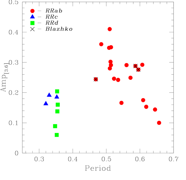
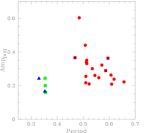
Figure 7: Period-amplitude (Bailey) diagrams in the 3.6 (upper panel) and 4.5 $\mu m$ (lower panel) passbands defined respectively by 28 and 24 RRLs in our sample, for which the determination of the amplitude with GRATIS was possible. Red circles, blue triangles and green squares represent RRab, RRc and RRd stars, respectively. Stars possibly affected by the Blazhko effect are marked by black crosses.

In order to clean our sample from blended sources and other contaminants we analysed the position of the RRLs on the CMDs shown in Fig. 3 and the light curves (Fig. 5) in combination with a visual inspection of the Spitzer images (Fig 4). Fig. 3 demonstrates that most of the variables conform to the RRc stars (blue triangles) being bluer than the RRab variables (red filled circles), and the RRd stars (green squares) being located between RRc and RRab stars. However, for five objects, namely, V01, V08, V19, V23 and V24 the position on the CMD is unusual. V08 is far too bright and red in colour than the bulk of the RRab stars. The star light curves are noisy, especially in the 4.5 $\mu m$ band (Fig. 5). Inspection of the Spitzer images showed that V08 is among an unresolved group of sources. V01 is slightly separated and fainter than other RRLs in the CMD. Moreover, V01 has a significantly redder colour than it would be expected for its period (P=0.51 days). The source is located on the upper edge of the 3.6 and 4.5 $\mu m$ images and does not have a characteristic stellar shape on the images, hence, the PSF photometry is likely not reliable. Star V23 is potentially a Blazhko variable and is slightly fainter than other RRLs, but the 3.6 and 4.5 $\mu m$ images and the star light curves do not have particular issues. The faint magnitude of this star may be consistent with its period (0.46863 days) that is the shortest among all the RRab stars in our sample. It is worth noting that V23 has also the faintest $V$ (Kuehn et al., 2013) magnitudes among all RRLs in Reticulum, which in combination with the results of this study may prove that V23 is indeed the intrinsically faintest star in the sample. While the faint MIR magnitudes can be explained by the shortest period of this star among all the RRab stars in the sample, the reason of the faint visual magnitude is unclear. A high metallicity of V23 could potentially account for its faint $V$ magnitude, however, it would contradict the general picture of Reticulum being monometallic cluster. Spectroscopical analysis of RRLs in Reticulum can shed light on this issue in the future. An alternative possibility is that V23 is a foreground RRL belonging to the field of the LMC. Star V19 has a too blue colour for an RRab variable. Moreover, it has a rather noisy light curve especially in the 4.5 $\mu m$ band. Visual inspection of the images showed that V19 has a companion with 3.6 $\mu m$ apparent magnitude 18 mag at a distance of 0.82 arcsec. The source is also located close to the edge of the 4.5 $\mu m$ image. Both these issues may have affected the photometry. V24 appears too red in colour for a RRd star and has an extremely noisy light curve. The star is located at a distance of 3.79 arcsec from a 15 mag bright source, with which it is blended in both passbands. Finally, V28 and V32 are not separated from the other RRLs on the CMD, but have noisy light curves. V28 has a close companion (at a distance of 1.63 arcsec) of magnitude $\sim 19$ mag, while V32 is blended by a companion with magnitude 18 mag located at a distance of 1.87 arcsec. Two further stars (V04 and V12) have noisy light curves but their images and the position on the CMD do not indicate any clear issue. V04 is a double mode pulsator and V12 is the shortest period (and hence faint) RRL in our sample. This may explain the noisy light curves. To summarise, the following six stars were dropped: V01, V08, V19, V24, V28, V32, while V04 and V12 were retained to avoid biasing our derivation of the $PL$ relations by brighter/longer period stars. Therefore in the following analysis we used a subsample of 24 RRLs consisting of 17 RRab, 3 RRc and 4 RRd stars.

3 MIR $PL$ relations

3.1 Slope of the PL relations.

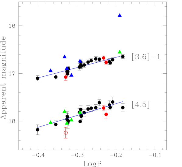
Figure 8: $PL$ relations in the 3.6 and 4.5 $\mu m$ passbands defined by the Reticulum RRLs. Filled circles represent RRLs used in the fit, with the Blazhko variables highlighted in red. Blue and green triangles show six RRLs that were discarded from the fit of respectively 3.6 and 4.5 $\mu m$ $PL$ relations as a results of the analysis of the light curves, position on the CMD and Spitzer images (Section 2.2). Star V23 was also discarded from the fit of the 4.5 $\mu m$ $PL$ relation by 3-sigma clipping procedure and is marked with a red empty circle (see text for details).

Figure 9: $PL$ relations in the 3.6 (upper panel) and 4.5 $\mu m$ (lower panel) passbands of five Galactic RRLs with the zero points calibrated using the HST parallaxes of Benedict et al. (2011). The logarithm of the period of RZ Cep was “fundamentalized” (Eq. 3). Slopes are from the present study (Eqs. 4-5). The fits were performed in parallax space. See text for details.

Figure 10: Same as in Fig. 9, but with the $PL$ zero points calibrated using TGAS parallaxes for the five Galactic RRLs. See Section 3.2 for details.

Figure 11: Same as in Fig. 9, but with the $PL$ zero points calibrated using DR2 parallaxes for the four Galactic RRLs and TGAS parallax for RR Lyr itself. See Section 3.2 for details.

A number of studies indicate a decreasing dependence of the RRL luminosity on metallicity when moving to longer wavelengths. A rather small metallicity dependence of the $K$-band luminosity has been found by empirical studies (see table 3 in Muraveva et al. 2015 for a summary), while theoretical studies suggest the dependence of the $K$-band luminosity on metallicity to be non-negligible (Bono et al. 2001, Catelan et al. 2004, Marconi et al. 2015), which recently was also confirmed by Braga et al. (2018) based on the analysis of RRLs in the GC $\omega$ Cen. The MIR $PL$ relations were derived neglecting the dependence of the luminosity on metallicity in a number of studies (e.g. Madore et al. 2013; Klein et al. 2014; Neeley et al. 2015, Gaia Collaboration et al. 2017). At the same time, some theoretical (Neeley et al., 2017) and empirical (Dambis et al. 2014, Sesar et al. 2017, Muraveva et al. 2018) studies suggest a non-negligible dependence of the MIR luminosity on metallicity (metallicity slope $\geq 0.1$ mag/dex, see Table 3). The RRLs analysed in this paper share the same metal abundance, hence, they cannot be used to estimate the effect of metallicity on the MIR $PL$ relations, however, we urge the reader to keep in mind a possible dependence of the MIR luminosity on metallicity.

Before we fit the MIR $PL$ relations, we corrected the apparent 3.6 and 4.5 $\mu m$ magnitude of the RRLs in our sample for interstellar extinction. Reddening $E(B-V)$ values towards the Reticulum cluster reported in the literature are generally low but controversial, and span the range from 0.016 mag (Schlegel et al., 1998) to 0.06 mag (Marconi et al., 2002). The range of reddening values for Reticulum reported in the literature implies an uncertainty in the $V$ magnitude, and therefore its distance estimation, of $\sim$ 0.14 mag. The situation improves significantly when moving to the MIR passbands, as the full range in reddening values reported in the literature causes uncertainties of only 0.009 and 0.007 mag in the 3.6 and 4.5 $\mu m$ bands, respectively, which are negligible in comparison with other uncertainties. In this paper we adopt the reddening value $E(B-V)=0.03\pm 0.02$ mag from Walker (1992), who estimated the reddening from the colours of the RRab stars at minimum light and Sturch’s method (Sturch 1966, Walker 1990). This value of the reddening is close to the mean of the reddening estimates in the literature. The following relations obtained by Monson et al. (2012) based on the reddening laws from Cardelli et al. (1989) and Indebetouw et al. (2005), were used to estimate the interstellar extinctions:

$$A_{[3.6]}=0.203*E(B-V)$$ (1)

$$A_{[4.5]}=0.156*E(B-V)$$ (2)

and derive the extinction values of 0.006 and 0.005 mag in the 3.6 and 4.5 $\mu m$ bands, respectively. The reddening-corrected 3.6 and 4.5 $\mu m$ magnitudes were then used to fit the MIR $PL$ relations.

We used the weighted least squares method and a 3-sigma clipping procedure to fit the $PL$ relations in the 3.6 and 4.5 $\mu m$ passbands defined by the RRLs in our sample. Following Dall’Ora et al. (2004) the RRd variables were treated as RRc stars. Periods of first-overtone and double-mode RRLs were then “fundamentalized” according to the relation:

$$\log(P)=\log(P_{fo})+0.127,$$ (3)

where $P_{fo}$ is the first-overtone period. The following $PL$ relations were derived:

$$[3.6]=(-2.15\pm 0.23)\times\log(P)+(17.23\pm 0.06)$$ (4)

with rms=0.06 mag,

$$[4.5]=(-2.47\pm 0.32)\times\log(P)+(17.14\pm 0.09)$$ (5)

with rms=0.07 mag,
where [3.6] and [4.5] are the absorption-corrected apparent magnitudes. The best fit relations are shown in Fig. 8, plotting with filled circles the RRLs used to fit the $PL$ relations, highlighting in red the Blazhko variables and marking with green and blue triangles six stars that were discarded when fitting the 4.5 and 3.6 $\mu m$ $PL$ relations, respectively, according to the analysis described in Section 2.2. We also note that star V23 was automatically rejected by the 3-sigma clipping procedure when fitting the $PL$ relation in the 4.5 $\mu m$ passband, which therefore is based on only 23 RRLs. We have marked this star with an empty circle in Fig. 8.

3.2 Zero point calibration

Table 3: Comparison of MIR period-luminosity-(metallicity) relations in the form $\alpha\times\log(P)+\beta\times{\rm[Fe/H]}+ZP$

.

Reference	Band	$\alpha$	$\beta$	$ZP$	$ZP$	$ZP$	$ZP$ from
				from HST $\varpi$	from TGAS $\varpi$	from Gaia DR2 $\varpi$	other sources
$PL$ relations ($W1$, [3.6])
This paper	3.6 $\mu m$	$-2.150\pm 0.230$	$-$	$-1.190\pm 0.050$	$-1.090\pm 0.090$	$-1.080\pm 0.03$	$-$
Madore et al. (2013)	$W1$	$-2.440\pm 0.950$	$-$	$-1.260\pm 0.250$	$-$	$-$	$-$
Klein et al. (2014) RRab	$W1$	$-2.380\pm 0.200$	$-$	$-$	$-$	$-$	$-1.113\pm 0.013^{a}$
Klein et al. (2014) RRc	$W1$	$-1.640\pm 0.620$	$-$	$-$	$-$	$-$	$-1.042\pm 0.031^{a}$
Neeley et al. (2015)	3.6 $\mu m$	$-2.332\pm 0.106$	$-$	$-1.176\pm 0.080$	$-$	$-$	$-1.054\pm 0.020^{b}$
Gaia Collaboration et al. (2017)	$W1$	$-2.440$	$-$	$-$	$-1.210\pm 0.040$	$-$	$-$
Neeley et al. (2017)	3.6 $\mu m$	$-2.300\pm 0.110$	$-$	$-1.112\pm 0.089$	$-$	$-$	$-$
$PLZ$ relations ($W1$, [3.6])
Dambis et al. (2014)	$W1$	$-2.381\pm 0.097$	$0.096\pm 0.021$	$-1.150\pm 0.077$	$-$	$-$	$-0.829\pm 0.093^{c}$
Neeley et al. (2017)	$W1$	$-2.247\pm 0.018$	$0.180\pm 0.003$	$-$	$-$	$-$	$-0.790\pm 0.007^{d}$
Neeley et al. (2017)	3.6 $\mu m$	$-2.251\pm 0.018$	$0.180\pm 0.003$	$-$	$-$	$-$	$-0.793\pm 0.007^{d}$
Sesar et al. (2017)	$W1$	$-2.470^{+0.74}_{-0.73}$	$0.150^{+0.09}_{-0.08}$	$-$	$-0.890^{+0.12}_{-0.10}$e	$-$	$-$
Muraveva et al. (2018)	$W1$	$-2.450^{+0.88}_{-0.82}$	$0.160^{+0.10}_{-0.10}$	$-$	$-$	$-0.910^{+0.36}_{-0.34}$	$-$
$PL$ relations ($W2$, [4.5])
This paper	4.5 $\mu m$	$-2.470\pm 0.320$	$-$	$-1.290\pm 0.050$	$-1.200\pm 0.080$	$-1.200\pm 0.030$	$-$
Madore et al. (2013)	$W2$	$-2.550\pm 0.890$	$-$	$-1.290\pm 0.230$	$-$	$-$	$-$
Klein et al. (2014) RRab	$W2$	$-2.390\pm 0.200$	$-$	$-$	$-$	$-$	$-1.110\pm 0.013^{a}$
Klein et al. (2014) RRc	$W2$	$-1.700\pm 0.620$	$-$	$-$	$-$	$-$	$-1.057\pm 0.031^{a}$
Neeley et al. (2015)	4.5 $\mu m$	$-2.336\pm 0.105$	$-$	$-1.199\pm 0.080$	$-$	$-$	$-1.091\pm 0.020^{b}$
Neeley et al. (2017)	4.5 $\mu m$	$-2.340\pm 0.100$	$-$	$-1.139\pm 0.089$	$-$	$-$	$-$
$PLZ$ relations ($W2$, [4.5])
Dambis et al. (2014)	$W2$	$-2.269\pm 0.127$	$0.108\pm 0.021$	$-1.105\pm 0.077$	$-$	$-$	$-0.776\pm 0.093^{c}$
Neeley et al. (2017)	$W2$	$-2.237\pm 0.018$	$0.185\pm 0.003$	$-$	$-$	$-$	$-0.784\pm 0.007^{d}$
Neeley et al. (2017)	4.5 $\mu m$	$-2.239\pm 0.018$	$0.185\pm 0.003$	$-$	$-$	$-$	$-0.785\pm 0.007^{d}$
Sesar et al. (2017)	$W2$	$-2.400^{+0.84}_{-0.82}$	$0.170^{+0.10}_{-0.09}$	$-$	$-0.947^{+0.11}_{-0.10}$e	$-$	$-$

^a Zero point derived from the $M_{V}-{\rm[Fe/H]}$ relation of RRLs in combination with the $\it HST$ parallaxes of RRLs in Benedict et al. (2011).
^b Zero point calibrated by adopting the distance modulus of the GC M4.
^c Zero point determined from the statistical-parallax analysis.
^d Theoretically determined zero point.
^e Zero point is from table 1 and eq. 4 in Sesar et al. (2017), assuming $P_{ref}=0.52854$ days and ${\rm[Fe/H]}_{ref}=-1.4$ dex.

To transform to absolute magnitudes the apparent magnitudes in Eqs. 4 and 5 we must calibrate the zero points of the $PL$ relations. Trigonometric parallaxes are the only direct method to estimate distances and infer absolute magnitudes. Until recently accurate parallax measurements were available for only a handful of RRLs. The ESA mission Hipparcos (van Leeuwen 2007 and references therein) measured the parallax for more than 100 RRLs in the solar neighbourhood, but with errors larger than 30%, except for RR Lyr itself, the bright prototype of the RRL class, for which the error is $\sim 18$%. Benedict et al. (2011) measured accurate trigonometric parallaxes of five Galactic RRLs (among which is RR Lyr) using the FGS on board the HST. However, we note that the Hipparcos and $HST$ parallax of RR Lyr are only in marginal agreement. Therefore, a direct calibration of the RRL distance relations has so far been hampered not only by a lack of good quality parallax data, but also by the few independent measurements presently available providing inconsistent results. Gaia, the ESA cornerstone mission launched on 2013 December 19, is measuring trigonometric parallaxes (along with positions, proper motions, photometry and physical parameters) for over one billion stars in the MW and beyond. Gaia will revolutionise the field by providing end-of-mission parallax measurements with about 10 $\mu as$ uncertainty for RRLs brighter than $V\sim$ 12-13 mag.

A first anticipation of Gaia promise in this field came on 2016 September 14 with the publication of the Gaia DR1 (Gaia Collaboration et al. 2016a, Gaia Collaboration et al. 2016b). The DR1 catalogue contains parallaxes for about 2 million stars in common between Gaia and the Hipparcos and Tycho-2 catalogues, computed as part of the TGAS (Lindegren et al., 2016). The TGAS sample includes parallaxes for 364 MW RRLs, of which a fraction was used by Gaia Collaboration et al. (2017) to calibrate the RRL visual $M_{V}-{\rm[Fe/H]}$ relation and the infrared $PL$ and $PLZ$ relations. Even though TGAS parallaxes for RRLs show an extraordinary improvement with respect to Hipparcos (see e.g. figure 23 in Gaia Collaboration et al. 2017), their uncertainties are still large, spanning from 0.209 to 0.967 mas in range. The situation improved significantly on 2018 April 25, when the Gaia trigonometric parallaxes for a much larger sample of RRLs using only Gaia measurements were published in Gaia DR2. The Gaia DR2 catalogue comprises positions and multi-band photometry for $\sim 1.7$ billion sources alongside the parallaxes and proper motions for $\sim 1.3$ billion sources (Gaia Collaboration et al., 2018). Furthermore, Gaia DR2 published a catalogue of more than $\sim$500,000 variables of different types (Holl et al., 2018), including 140,784 RRLs (Clementini et al., 2018). The dramatic improvement brought by Gaia DR2 for RRLs, compared to its precursors Hipparcos and Gaia DR1, is demonstrated in figure 6 of Muraveva et al. (2018).

We retrieved Gaia DR2 parallaxes for the 30 RRLs in Reticulum from the Gaia Archive website. The resulting values are shown in Table 2. Unfortunately, owing to the large distances and faint magnitudes of the RRLs in Reticulum (mean Gaia $G$-band magnitude $<G>=19.02$ mag), 50% of the Reticulum RRLs have negative parallax values, while the remaining 15 RRLs have large relative parallax uncertainties ($<\sigma_{\varpi}/\varpi>=2.7$). Consequently, the Reticulum sample is unsuitable for calibrating the zero points of the RRL MIR $PL$ relations. Instead we adopt the slope of the MIR $PL$ relations derived for the RRLs in Reticulum (Eqs. 4 and 5), and calibrate the zero points using the parallaxes of RRLs in the MW. We selected the HST parallaxes for the five RRLs in Benedict et al. (2011) and the TGAS and Gaia DR2 parallaxes for the same stars, and then compared the resulting $PL$ relations with the literature relations (Section 3.3).

Apparent magnitudes in the Spitzer passbands for the five MW RRLs with HST parallaxes published by Benedict et al. (2011), namely, RZ Cep, XZ Cyg, SU Dra, RR Lyr and UV Oct, are provided in table 5 of Neeley et al. (2015), HST parallaxes are taken from table 8 of Benedict et al. (2011) and the TGAS and Gaia DR2 parallaxes are retrieved from Gaia Archive website but they are also listed in table 1 of Gaia Collaboration et al. (2017), for TGAS, and table 2 of Muraveva et al. (2018), for the DR2 parallaxes. Periods of these five stars range from 0.3086 to 0.6604 days and metallicities span the range from [Fe/H]=$-$1.80 to $-$1.41 dex on the Zinn & West (1984) metallicity scale. The metallicity of the RRLs in Reticulum is [Fe/H]=$-$1.66 dex on the Zinn & West (1984) metallicity scale (Mackey & Gilmore, 2004), which is well within the range spanned by Benedict et al. (2011)’s variables. The logarithm of the RRc star RZ Cep was “fundamentalized” (Eq. 3).

The DR2 parallax for RR Lyr itself has a large negative value ($-2.61\pm 0.61$ mas) and is clearly wrong (Arenou et al. 2018, Gaia Collaboration et al. 2018). Hence, for this star we adopt the TGAS parallax instead of the DR2 measure.

As widely discussed in Gaia Collaboration et al. (2017), the direct transformation of parallaxes into absolute magnitudes using the relation:

$$M=m_{0}+5\log\varpi-10,$$ (6)

where M is the star absolute magnitude, $m_{0}$ is the dereddened apparent magnitude and $\varpi$ is the parallax in mas, has significant disadvantages. While errors in parallaxes are approximately Gaussian and symmetrical, the logarithm in Eq. 6 causes the errors in absolute magnitudes to become asymmetrical leading to biased results (Gaia Collaboration et al. 2017; Luri et al. 2018). Furthermore, using this method means that negative parallaxes cannot be transformed into absolute magnitudes which causes a truncation bias in the data. In order to circumvent both issues it is advisable to operate directly in the parallax space, using, for instance, the reduced parallax (Feast & Catchpole, 1997) or Astrometry-Based Luminosity (ABL, Arenou & Luri 1999) method that is defined by the relation:

$$ABL=10^{0.2M}=10^{0.2(\alpha\log P+ZP)}=\varpi 10^{0.2m_{0}-2},$$ (7)

where M is the stars absolute magnitude, P is the period, $m_{0}$ is the dereddened apparent magnitude, $\varpi$ is the parallax in mas, $\alpha$ is the slope of the $PL$ relation, for which we adopt the values we have derived from the RRLs in Reticulum (Eqs. 4 and 5 in Section 3.1), and $ZP$ is the $PL$ zero point that we aim to determine. Using the ABLs instead of the absolute magnitudes for our RRL calibrators allows us to maintain symmetrical errors. We also note that there is no need to apply any Lutz - Kelker correction (Lutz & Kelker, 1973) in our study, since individual measurements of objects that were chosen independently of their parallax values or relative errors in parallaxes are not affected by the Lutz - Kelker bias (Arenou & Luri 1999, Feast 2002), and indeed the five RRLs in Benedict et al. (2011) were not selected based on their observed parallaxes.

A number of independent studies regarding a possible zero point offset of Gaia DR2 parallaxes appeared recently in literature (e.g. Arenou et al. 2018; Riess et al. 2018; Zinn et al. 2018; Stassun & Torres 2018; Muraveva et al. 2018). All these studies indicate that the Gaia DR2 parallaxes are systematically smaller with a mean estimated offset of $\Delta\varpi=-0.03~{}mas$ (Arenou et al., 2018). Arenou et al. (2018) do not recommend to correct for this possible parallax offset individual star parallaxes. Hence, we did not apply this correction to the five MW RRLs in our study.

The resulting 3.6 and 4.5 $\mu m$ $PL$ fits obtained by using the HST, TGAS and DR2 parallaxes of the five MW RRL calibrators are shown in Figs. 9, 10 and 11, respectively. The fits were performed in parallax space, with parallaxes later transformed to absolute magnitudes in order to visualise the data on the $PL$ plane. The slopes and zero points of the fits are listed in Table 3.

3.3 Comparison with the literature

In recent years, several authors have studied the RRL MIR $PL$ relations. These literature relations were calibrated either using the trigonometric parallaxes or by indirect methods to determine the zero point. Here, we briefly summarise these previous studies with a specific focus on the adopted calibration procedures. In Table 3 we present the literature slopes and zero points alongside the values derived in the present study.

Madore et al. (2013) used Wide-field Infrared Survey Explorer (WISE) observations in the $[W1]$ (3.4 $\mu$m), $[W2]$ (4.6 $\mu$m) and $[W3]$ (12 $\mu$m) passbands for the four fundamental mode RRLs in Benedict et al. (2011) (they excluded the first-overtone star RZ Cep) to derive $PL$ relations in the WISE MIR passbands directly calibrated on the HST parallaxes of the stars.

Similarly, Dambis et al. (2014) derived metallicity-dependent MIR $PLZ$ relations using WISE $W1$ observations for 360 RRLs in 15 MW GCs and $W2$ observations for 275 RRLs in 9 GCs. The authors calibrated the zero points in two different ways: based on a statistical-parallax analysis and using the HST parallaxes of the four RRLs in Madore et al. (2013). The corresponding zero points differ by more than 0.3 mag, with the statistical-parallax calibration providing fainter absolute magnitudes. $PL$ relations in the WISE $W1$, $W2$ and $W3$ passbands were derived also by Klein et al. (2014) for RRab and RRc stars separately, using 129 field MW RRLs whose distances were inferred from the ${M_{V}-{\rm[Fe/H]}}$ relation in Chaboyer (1999) calibrated with Benedict et al. (2011)’s trigonometric parallaxes.

Neeley et al. (2015) derived $PL$ relations in the 3.6 and 4.5 $\mu m$ passbands using 37 RRLs observed with Spitzer IRAC in the GC M4. The zero point calibration was obtained combining the HST parallaxes with the Spitzer photometry of the 5 RRLs in Benedict et al. (2011) observed as part of the CRRP and, as an alternative, by adopting the distance to M4 from Braga et al. (2015). New theoretical $PLZ$ relations in the Spitzer and WISE passbands were published by Neeley et al. (2017) who also revised the empirical relations in Neeley et al. (2015) using M4 data reduced with a new Spitzer pipeline.

Gaia Collaboration et al. (2017) calibrated their own $PL$ relation in the $W1$ passband using the TGAS parallaxes of 198 MW RRLs and adopting the slope from Madore et al. (2013). Gaia Collaboration et al. (2017) used three different approaches to infer the zero point of the $PL$ relations. In Table 3 we list the zero point derived using the ABL (Arenou & Luri 1999), which is also the procedure adopted to calibrate the $PL$ relations derived in the present paper.

Sesar et al. (2017) studied a sample of about 100 MW RRab stars and calibrated the MIR $W1$ and $W2$ $PLZ$ relations based on TGAS parallaxes. Recently, Muraveva et al. (2018) derived new $W1$-band $PLZ$ relations using Gaia DR2 parallaxes for a sample of 401 MW RRL variables and for a reduced sample of 23 nearby RRLs whose metallicity was estimated from high-resolution spectroscopy. The MIR relation obtained by Muraveva et al. (2018) using the sample of 23 nearby RRLs after correcting for a Gaia DR2 parallax offset of 0.056 mas is shown in Table 3. For ease of comparison in Table 3 we grouped the $PL$ and $PLZ$ relations in the $W1$ and 3.6 $\mu m$ passbands, and those in the $W2$ and 4.5 $\mu m$ bands, since they are very similar.

The slope of the $PL$ relation in the 3.6 $\mu m$ band derived in this paper is shallower than values published in previous studies but still consistent with them within the errors. The slope of the $PL$ relation in 4.5 $\mu m$ passband is in very good agreement, within the quoted uncertainties, with all previous studies. The absolute magnitudes based on the TGAS and DR2 parallaxes are in very good agreement to each other and generally fainter than those based on the HST parallaxes. In Section 4 we discuss the distance to Reticulum inferred from the new $PL$ relations and their different calibration procedures.

Table 4: Comparison of the distance moduli for Reticulum derived in the present study and literature values.

Reference	Band	$E(B-V)$	Distance modulus
		(mag)	(mag)
Demers & Kunkel (1976)	$V$	0.02	18.51
Walker (1992)	$V$	0.03	18.38
Ripepi et al. (2004)	$V$	0.02	$18.39\pm 0.12$
Mackey & Gilmore (2004)	$V$	0.05	$18.39\pm 0.12$
Kuehn et al. (2013)	$V$	0.016	$18.40\pm 0.20$
Jeon et al. (2014)	$V$	0.03	18.40
Sollima et al. (2008)	$V$	0.03	$18.44\pm 0.14$
Kuehn et al. (2013)	$I$	0.016	$18.47\pm 0.06$
Dall’Ora et al. (2004)	$K$	0.03	$18.52\pm 0.05\pm 0.117$
Sollima et al. (2008)	$K$	0.03	$18.48\pm 0.11$
This paper (HST)	[3.6]	0.03	$18.43\pm 0.06$
This paper (TGAS)	[3.6]	0.03	$18.33\pm 0.06$
This paper (DR2)	[3.6]	0.03	$18.32\pm 0.06$
This paper (HST)	[4.5]	0.03	$18.43\pm 0.08$
This paper (TGAS)	[4.5]	0.03	$18.34\pm 0.08$
This paper (DR2)	[4.5]	0.03	$18.34\pm 0.08$

4 Distance to Reticulum

Several independent estimates of the distance to Reticulum are available in the literature. Table 4 summarises the distances derived in this study and other key works. We indicate the photometric passbands and the reddening values used in the various analyses.

Demers & Kunkel (1976) derived a distance modulus for Reticulum of $\mu=18.51$ mag using the mean apparent $V$ magnitudes of the HB stars. These authors also found that the mean $B$ magnitude of the RRLs in Reticulum is about 0.15 mag brighter than for RRLs in the LMC field. Several independent studies, such as Freedman et al. (2001) based on classical Cepheids, Clementini et al. (2003) using RRLs and Pietrzyński et al. (2013) from a sample of eight eclipsing binaries, have shown that the distance to the LMC is $\mu\sim 18.50$ mag (see e.g de Grijs et al. 2014 for a compilation of literature values). Therefore, the 0.15 mag difference in mean $B$ magnitude found by Demers & Kunkel (1976) implies $\mu\sim 18.35$ mag for the distance modulus of Reticulum, assuming that the reddening and $B$ absolute magnitude are the same in the two systems.

Walker (1992), Ripepi et al. (2004), Mackey & Gilmore (2004), Kuehn et al. (2013) derived the distance to Reticulum from the $V$-band observations of the 32 RRLs in the cluster. Kuehn et al. (2013) also derived a distance modulus for Reticulum using their $I$-band photometry of the cluster RRL variables, individual metallicities estimated from the Fourier parameters of the light curves and adopting the $PLZ$ relation of Catelan et al. (2004). Jeon et al. (2014) derived the distance to Reticulum by fitting theoretical isochrones to the cluster $V$ versus ($B-V$) CMD. All distance moduli based on the $V$ photometry agree on a distance modulus value around $\mu=18.40$ mag, except Demers & Kunkel (1976)’s that is about 0.1 mag larger.

Dall’Ora et al. (2004) combined the apparent $K$-band magnitudes of 30 RRLs in Reticulum with the theoretical $PLZ$ relation by Bono et al. (2003) obtaining the distance modulus $\mu=18.52\pm 0.005(random)\pm 0.117(systematic)$ mag which is about 0.1 mag larger than that derived from the $V$ photometry. These authors made a detailed analysis of possible systematic uncertainties affecting their analysis. Distances obtained from the NIR $PLZ$ relation were found to be systematically larger than distances derived from Baade-Wesselink studies (Fernley, 1994), with the difference ranging from $\delta\mu=0.10$ mag for more metal-rich clusters to $\delta\mu=0.32$ mag for more metal-poor clusters. Therefore, the distance modulus of $\mu=18.52$ mag derived from the $K$-band photometry of Reticulum could be an overestimate. Later, Sollima et al. (2008) also found that the distance to Reticulum derived from the $K$-band photometry of Dall’Ora et al. (2004) is 0.04 mag larger than the distance inferred from the $V$-band photometry of Walker (1992).

A comparison of the values in Table 4 indeed confirms that distances based on $K$- and $I$-band photometry are in general larger than distances derived from the optical photometry, which could suggest some issues in the zero point calibrations in the two different passbands.

In this study we obtained distance moduli for Reticulum by applying our $PL$ relations to estimate individual distances to each of the 24 and 23 RRLs used in our analysis of the 3.6 $\mu m$ and 4.5 $\mu m$ $PL$ relations, respectively, then averaging the resulting values. Errors are the standard deviations from the average. We obtained the following distance moduli for Reticulum: $\mu_{[3.6]}=18.43\pm 0.06$ mag and $\mu_{[4.5]}=18.43\pm 0.08$ mag from the $PL$ relations calibrated on the HST parallaxes; $\mu_{[3.6]}=18.33\pm 0.06$ mag and $\mu_{[4.5]}=18.34\pm 0.08$ mag using the TGAS parallaxes and $\mu_{[3.6]}=18.32\pm 0.06$ mag and $\mu_{[4.5]}=18.34\pm 0.08$ mag using the DR2 parallaxes. These values are also reported in the bottom part of Table 4. The distance moduli estimated using the $PL$ relations calibrated on the HST parallaxes are in good agreement with the majority of the literature estimates, especially with those based on the $V$ photometry. Distance moduli obtained from the $PL$ relations calibrated on the TGAS and DR2 parallaxes are generally smaller, but still consistent within errors with the majority of previous estimates.

Pietrzyński et al. (2013) estimated a distance to the LMC of $D=49.97\pm 0.19$ (stat) $\pm$ 1.11 (syst) kpc ($\mu_{0}$= 18.493 $\pm$ 0.008 (stat) $\pm$ 0.047 (syst) mag) from eight long-period eclipsing binary systems which are all located relatively close to the barycentre of the LMC. Taking the mean value of all six distance moduli derived in this study we conclude that Reticulum is located approximately 3 kpc closer to us than the barycentre of the LMC.

5 Summary

We have analysed a sample of 30 RRLs in the LMC cluster Reticulum that we observed in the 3.6 and 4.5 $\mu m$ passbands with IRAC in the Spitzer Warm Cycle 9 as part of the CRRP. Observations consist of 12 epochs over a $\sim 14$ hours time span, allowing a good coverage of the RRL light curves. We analysed the light curves with the GRATIS software to derive MIR characteristic parameters (amplitudes and intensity-averaged mean magnitudes). We combined our MIR data with optical photometry from Jeon et al. (2014), and the resulting CMDs show a well defined RGB, an HB well populated by the cluster RRLs and a few variables with magnitude/colour affected by crowding. Based on our analysis of the light curves, the position on the CMD and the appearance on the images we selected a sample of 24 RRLs that we used to fit the MIR $PL$ relations. The slope of the $PL$ relation in 3.6 $\mu m$ passband derived in this paper ($-2.15\pm 0.23$) is shallower than the values published in previous studies but still consistent within the errors. The slope of the $PL$ relation in the 4.5 $\mu m$ passband ($-2.47\pm 0.32$), based on the 23 RRLs remained after the 3-sigma clipping procedure, is in very good agreement, within the errors, with the literature studies.

To estimate the zero points of our MIR $PL$ relations we used five MW RRLs for which trigonometric parallaxes were measured with the HST FGS (Benedict et al., 2011), Gaia as part of TGAS in Gaia DR1 and Gaia DR2, based only on Gaia measurements, allowing us to make a direct comparison of the three calibrations. We used the ABL method to fit the MIR RRL $PL$ relations, as this operates directly in parallax space, avoiding non-symmetrical errors in absolute magnitudes caused by inversion of the parallaxes. We found that the absolute magnitudes based on the TGAS and DR2 parallaxes are in good agreement with each other and are in general fainter than those based on the HST parallaxes. However, the sample of RRLs used in the analysis is too small to draw any conclusion about possible systematic offsets.

We obtained the following distance moduli for Reticulum: $\mu_{[3.6]}=18.43\pm 0.06$ mag and $\mu_{[4.5]}=18.43\pm 0.08$ mag from the $PL$ relations calibrated on the HST parallaxes; $\mu_{[3.6]}=18.33\pm 0.06$ mag and $\mu_{[4.5]}=18.34\pm 0.08$ mag using the TGAS parallaxes and $\mu_{[3.6]}=18.32\pm 0.06$ mag and $\mu_{[4.5]}=18.34\pm 0.08$ mag using the DR2 parallaxes. These distance moduli are in good agreement with the literature values estimated using the $V$ band photometry, while the agreement with the distance values of Reticulum based on the $I$ and $K$ photometry is less pronounced.

Based on the mean of the distance moduli derived in this study we conclude that Reticulum is located approximately 3 kpc closer to us than the barycentre of the LMC.

References

- Arenou & Luri (1999) Arenou F. & Luri X., 1999, Harmonizing Cosmic Distance Scales in a Post-HIPPARCOS Era, 167, 13
- Arenou et al. (2018) Arenou F. et al., 2018, arXiv:1804.09375
- Benedict et al. (2011) Benedict G. F. et al., 2011, AJ, 142,187
- Bica et al. (1999) Bica E. L. D., Schmitt H. R., Dutra C. M., Oliveira, H. L. 1999, AJ, 117, 238
- Blaẑko (1907) Blaẑko S., 1907, AN, 175, 327
- Bono et al. (2001) Bono G., Caputo F., Castellani V., Marconi M., Storm J., 2001, MNRAS, 326, 1183
- Bono et al. (2003) Bono G., Caputo F., Castellani V., Marconi M., Storm J., Degl’Innocenti S., 2003, MNRAS, 344, 1097
- Braga et al. (2015) Braga V. F. et al., 2015, ApJ, 799, 165
- Braga et al. (2018) Braga V. F. et al., 2018, AJ, 155, 137
- Cardelli et al. (1989) Cardelli J. A., Clayton G. C., & Mathis, J. S., 1989, ApJ, 345, 245
- Catelan et al. (2004) Catelan M., Pritzl B. J. & Smith H. A. E. 2004, ApJS, 154, 633
- Caputo et al. (2000) Caputo F., Castellani V., Marconi M. & Ripepi V., 2000, MNRAS, 316, 819
- Chaboyer (1999) Chaboyer B., 1999, in Heck A., Caputo F., eds, Post-Hipparcos Cosmic Candles. Kluwer, Dordrecht, p. 111
- Clementini et al. (2000) Clementini G. et al., 2000, AJ, 120, 2054
- Clementini et al. (2003) Clementini G. et al., 2003, AJ, 125, 1309
- Clementini et al. (2018) Clementini G. et al., 2018, arXiv:1805.02079
- Dall’Ora et al. (2004) Dall’Ora M., Storm J., Bono. G. et al., 2004, ApJ, 610, 269
- Dambis et al. (2014) Dambis A. K., Rastorguev A. S. & Zabolotskikh M. V., 2014, MNRAS, 439, 3765
- de Grijs et al. (2014) De Grijs, R., Wicker J. E., & Bono, G., 2014, AJ, 147, 122
- Demers & Kunkel (1976) Demers S. & Kunkel W. E., 1976, ApJ, 208, 932
- Fazio et al. (2004) Fazio G. G., Hora J. L., Allen L. E. et al., 2004, ApJS, 154, 10
- Feast (2002) Feast M., 2002, MNRAS, 337, 1035
- Feast & Catchpole (1997) Feast M. W. & Catchpole R. M.,1997, MNRAS, 286, L1
- Fernley (1994) Fernley J., 1994, A&A, 284, L16
- Freedman et al. (2001) Freedman W. L., Madore B. F., Gibson B. K. et al, 2001, ApJ, 553, 47
- Freedman et al. (2011) Freedman, W. L., Madore B. F., Scowcroft V. et al., 2011, AJ, 142, 192