Enhancing the cross-correlations between magnetic fields and scalar perturbations through parity violation

Abstract

One often resorts to a non-minimal coupling of the electromagnetic field in order to generate magnetic fields during inflation. The coupling is expected to depend on a scalar field, possibly the same as the one driving inflation. At the level of three-point functions, such a coupling leads to a non-trivial cross-correlation between the perturbation in the scalar field and the magnetic field. This cross-correlation has been evaluated analytically earlier for the case of non-helical electromagnetic fields. In this work, we numerically compute the cross-correlation for helical magnetic fields. Non-Gaussianities are often generated as modes leave the Hubble radius. The helical electromagnetic modes evolve strongly (when compared to the non-helical case) around Hubble exit and one type of polarization is strongly amplified immediately after Hubble exit. We find that helicity considerably boosts the amplitude of the dimensionless non-Gaussianity parameter that characterizes the amplitude and shape of the cross-correlation between the perturbations in the scalar field and the magnetic field. We discuss the implications of the enhancement in the non-Gaussianity parameter due to parity violation.

1 Introduction

The observations of widely prevalent magnetic fields in the universe call for investigations into their origin. The amplitude of the magnetic fields vary over an extensive range, from a few micro Gauss in stars and galaxies, to around $10^{-17}$ Gauss in the intergalactic medium [1, 2, 3, 4, 5, 6, 7, 8, 9, 10] and the large scale structure [11, 12, 13, 14, 15, 16]. Additionally, observations of the anisotropies in the Cosmic Microwave Background (CMB) by Planck and POLARBEAR have led to an upper bound of a few nano Gauss on the magnetic fields at scales of $1\,{\rm Mpc}$ [17, 18]. It has been realized that such large scale magnetic fields may need to be generated primordially, which can then be amplified by astrophysical processes. For instance, magnetohydrodynamic (MHD) processes such as the dynamo mechanism in astrophysical systems necessarily require a seed field that can act as the progenitor of the observed magnetic fields [13, 14, 15, 19, 20, 16]. It has been conjectured that primordial magnetogenesis, i.e. generation of magnetic fields via quantum fluctuations in the early universe, can produce the precursor seed fields which can, over the course of time, source the large scale magnetic fields.

Inflation, on account of being the most appealing paradigm to describe the early universe, has also garnered tremendous interest as the framework for primordial magnetogenesis. However, the rapid decay of magnetic fields generated by the standard electromagnetic action in an expanding universe compels one to look for a means to circumvent this issue. One of the feasible ways to engender magnetic fields of appropriate strengths seems to be the introduction of a non-minimal coupling term in the action [21, 22]. Magnetic fields generated through breaking the conformal invariance of the standard electromagnetic action, due to the presence of a non-minimal coupling term, and with a suitable choice of the parameters involved, have been shown to be of the pertinent amplitude and correlation length to be in concordance with the observations [23, 24, 25, 26, 27, 28, 19, 29, 30, 31, 32, 33, 34, 35, 36, 37, 38, 39, 40].

In the context of primordial magnetogenesis, another interesting aspect is to study the magnetic fields generated due to the addition of a parity violating term to the standard electromagnetic action. Such a term would lead to the generation of the so-called helical magnetic fields [27, 30, 32, 41, 42]. In this situation, two modes with positive and negative helicity are generated, which evolve differently and, as a consequence, can conceivably lead to distinct imprints, such as correlations between B-mode and E-mode polarizations or the temperature and B-mode polarizations in the CMB [43, 44, 30]. They can also lead to the production of helical gravitational waves with possible observational imprints (in this context, see, for example, Refs. [43, 44, 45, 30]). Further, it has been shown that, the helical fields evolve strongly in the cosmic MHD plasma through an inverse cascade mechanism, resulting in an augmentation of the power on large scales [46, 47, 48].

An additional way to constrain these magnetic fields would be to study their cross-correlations at the level of the three-point functions with the scalar perturbations and their possible observational imprints. While such three-point functions have already been studied for the case of non-helical magnetic fields [49, 50, 51, 52], we believe it is of utmost interest to study the non-Gaussianities produced due to the helical fields as well. Analytically, the evaluation of these three-point functions seems to be a formidable task, due to the non-trivial form of the helical modes involving the Coulomb functions [30, 32, 41]. In this work, we shall numerically evaluate the three-point function involving the helical magnetic fields and the perturbations in an auxiliary scalar field and examine its implications.

This paper is structured as follows. In the next section, we shall discuss the action governing non-minimally coupled helical electromagnetic fields, their quantization and the power spectrum associated with the magnetic field. In Sec. 3, working with a specific form of the non-minimal coupling, we shall revisit the evaluation of the power spectrum of helical magnetic fields arising in de Sitter inflation. In Sec. 4, by suitably perturbing the action, we shall arrive at the Hamiltonian describing the interaction between the perturbed scalar field and the electromagnetic field. Using the interaction Hamiltonian, we shall arrive at the formal structure of the three-point function describing the cross-correlation between the perturbation in the scalar field and the electromagnetic field. In Sec. 5, we shall outline the numerical procedure that we shall adopt to compute the cross-correlation. In Sec. 6, we shall first compare our numerical results with the analytical results available in the non-helical case for two different situations (one leading to a power spectrum with a tilt and another which leads to a scale invariant spectrum) and present the corresponding results in the helical case. We shall conclude in Sec. 7 with a brief summary of the results we have obtained.

Note that, we shall work with natural units such that $\hbar=c=1$ and set the Planck mass to be $M_{{}_{\rm Pl}}=\left(8\,\pi\,G\right)^{-1/2}$. We shall adopt the metric signature of $\left(-,+,+,+\right)$. Greek indices shall denote the spacetime coordinates, whereas the Latin indices shall represent the spatial coordinates, except for $k$ which shall be reserved for denoting the wavenumber. Lastly, an overprime shall denote differentiation with respect to the conformal time coordinate.

2 Non-minimally coupled, helical electromagnetic fields, quantization and power spectrum

We shall consider the background to be the spatially flat, Friedmann-Lemaître-Robertson-Walker (FLRW) metric that is described by the line-element

$${\rm d}s^{2}=a^{2}(\eta)\,\left(-{\rm d}\eta^{2}+\delta_{ij}\,{\rm d}x^{i}\,{\rm d}x^{j}\right),$$ (2.1)

where $a(\eta)$ is the scale factor and $\eta$ denotes the conformal time coordinate. We consider the action [41]

$$S_{\rm em}[A^{\mu},\phi]=-\frac{1}{16\,\pi}\int{\rm d}^{4}x\,\sqrt{-g}\left[J^{2}(\phi)\,F_{\mu\nu}F^{\mu\nu}-\frac{\gamma}{2}\,I^{2}(\phi)\,F_{\mu\nu}{\tilde{F}^{\mu\nu}}\right],$$ (2.2)

where the electromagnetic field tensor is given by

$$F_{\mu\nu}=\partial_{\mu}\,A_{\nu}-\partial_{\nu}\,A_{\mu}.$$ (2.3)

The dual of the electromagnetic tensor ${\tilde{F}^{\mu\nu}}$ is defined as

$${\tilde{F}^{\mu\nu}}=\epsilon^{\mu\nu\alpha\beta}\,F_{\alpha\beta},$$ (2.4)

with $\epsilon^{\mu\nu\alpha\beta}=\left(1/\sqrt{-g}\right)\,{\cal A}^{\mu\nu\alpha\beta}$, where ${\cal A}^{\mu\nu\alpha\beta}$ is the totally antisymmetric Levi-Civita tensor and ${\cal A}^{0123}=1$. Clearly, the function $J(\phi)$ describes the non-minimal coupling, while the function $I(\phi)$ (along with the parameter $\gamma$) leads to parity violation.

We shall assume that there is no homogeneous component to the electromagnetic field. We shall choose to work in the Coulomb gauge wherein $A_{0}=0$ and $\partial_{i}\,A^{i}=0$. In such a gauge, at the quadratic order in the inhomogeneous modes, the action describing the electromagnetic field is found to be

$$S[A_{i}]=\frac{1}{4\,\pi}\,\int\,{\rm d}\,\eta\,\int\,{\rm d}^{3}\,\bm{x}\left\{J^{2}\left(\phi\right)\left[\frac{1}{2}\,A_{i}^{\prime\,2}-\frac{1}{4}\left(\partial_{i}\,A_{j}-\partial_{j}\,A_{i}\right)^{2}\right]+\gamma\,I^{2}\left(\phi\right)\,\epsilon^{ijk}\,A_{i}^{\prime}\,\partial_{j}\,A_{k}\right\},$$ (2.5)

where $\epsilon^{ijk}$ is the three-dimensional completely anti-symmetric tensor. We can vary this action to arrive at the following equation of motion for the electromagnetic vector potential:

$$A_{i}^{\prime\prime}+2\,\frac{J^{\prime}}{J}\,A_{i}^{\prime}-\nabla^{2}\,A_{i}=-\frac{\gamma}{J^{2}}\,\frac{{\rm d}I\,^{2}}{{\rm d}\,\eta}\,\delta_{il}\,\epsilon^{lnm}\,\partial_{n}\,A_{m}.$$ (2.6)

For each comoving wave vector $\bm{k}$, we can define the right-handed orthonormal basis $(\varepsilon_{1}^{\bm{k}},\varepsilon_{2}^{\bm{k}},\hat{\bm{k}})$, where

$$|\varepsilon^{\bm{k}}_{i}|^{2}=1,\quad\varepsilon^{\bm{k}}_{1}\times\varepsilon^{\bm{k}}_{2}=\hat{\bm{k}}\quad{\rm and}\quad\varepsilon^{\bm{k}}_{1}\cdot\varepsilon^{\bm{k}}_{2}=\hat{\bm{k}}\cdot\varepsilon^{\bm{k}}_{1}=\hat{\bm{k}}\cdot\varepsilon^{\bm{k}}_{2}=0.$$ (2.7)

While this is a suitable basis for expressing the non-helical modes, it is not ideally suited for the helical case as the two helical modes would be coupled in this basis. In such a situation, it is convenient to identify two transverse directions to form the helicity basis, wherein the modes decouple, as follows [30, 32]:

$$\varepsilon^{\bm{k}}_{\pm}=\frac{1}{\sqrt{2}}\left(\varepsilon^{\bm{k}}_{1}\pm i\,\varepsilon^{\bm{k}}_{2}\right).$$ (2.8)

In such a basis, on quantization, the vector potential $\hat{A_{i}}$ can be Fourier decomposed as [41]:

$${\hat{A}}_{i}(\eta,{\bm{x}})=\sqrt{4\,\pi}\int\frac{{\rm d}^{3}\,{\bm{k}}}{(2\,\pi)^{3/2}}\,\sum_{\sigma=\pm}\,\left[\varepsilon^{\bm{k}}_{\sigma i}\,\hat{b}_{\bm{k}}^{\sigma}\,{\bar{A}}_{k}^{\sigma}(\eta)\,{\rm e}^{i\,{\bm{k}}\cdot{\bm{x}}}+\varepsilon^{\bm{k}\,\ast}_{\sigma i}\,\hat{b}_{\bm{k}}^{\sigma\dagger}\,{\bar{A}}_{k}^{\sigma}(\eta)\,{\rm e}^{-i\,{\bm{k}}\cdot{\bm{x}}}\right],$$ (2.9)

where the Fourier modes ${\bar{A}}_{k}^{\sigma}$ satisfy the differential equation

$${\bar{A}}_{k}^{\sigma\,\prime\prime}+2\,\frac{J^{\prime}}{J}\,{\bar{A}}_{k}^{\sigma\,\prime}+\left(k^{2}+\frac{\sigma\,\gamma\,k}{J^{2}}\,\frac{{\rm d}I\,^{2}}{{\rm d}\,\eta}\right)\,{\bar{A}}_{k}^{\sigma}=0.$$ (2.10)

Note that $\sigma=\pm 1$, and this causes considerable difference in the evolution of the modes. As we shall see, one of the modes will be strongly amplified on super-Hubble scales and the extent of amplification will depend on the quantity $\gamma$. The operators $\hat{b}_{\bm{k}}^{\sigma}$ and $\hat{b}_{\bm{k}}^{\sigma\dagger}$ are the annihilation and creation operators satisfying the following standard commutation relations:

$$[{\hat{b}}_{\bm{k}}^{\sigma},\hat{b}_{\bm{k}^{\prime}}^{\sigma^{\prime}}]=[{\hat{b}}_{\bm{k}}^{\sigma\dagger},{\hat{b}}_{\bm{k}^{\prime}}^{\sigma^{\prime}\dagger}]=0\quad{\rm and}\quad[\hat{b}_{\bm{k}}^{\sigma},\hat{b}_{\bm{k}^{\prime}}^{\sigma^{\prime}\dagger}]=\delta^{(3)}({\bm{k}}-{\bm{k}^{\prime}})\,\delta_{\sigma\sigma^{\prime}}.$$ (2.11)

Let us define $\mathcal{A}_{k}^{\sigma}=J\,{\bar{A}}_{k}^{\sigma}$. In terms of the new variable $\mathcal{A}_{k}^{\sigma}$, Eq. (2.10) can be rewritten as

$$\mathcal{A}_{k}^{\sigma\,\prime\prime}+\left(k^{2}-\frac{J^{\prime\prime}}{J}+\frac{\sigma\,\gamma\,k}{J^{2}}\,\frac{{\rm d}I\,^{2}}{{\rm d}\,\eta}\right)\,\mathcal{A}_{k}^{\sigma}=0.$$ (2.12)

In this work, we shall restrict ourselves to the simplest scenarios wherein $I=J$. In such a case, the above equation simplifies to

$$\mathcal{A}_{k}^{\sigma\,\prime\prime}+\left(k^{2}-\frac{J^{\prime\prime}}{J}+\frac{2\,\sigma\,\gamma\,k\,J^{\prime}}{J}\right)\mathcal{A}_{k}^{\sigma}=0.$$ (2.13)

Since we shall be only interested in the behavior of the helical magnetic fields, we shall not discuss the electric field in this work. Let $\hat{\rho}_{{}_{\rm B}}$ denote the operator corresponding to the energy density associated with the magnetic field. Upon using the decomposition (2.9) of the vector potential, the expectation value of the energy density $\hat{\rho}_{{}_{\rm B}}$ can be evaluated in the vacuum state, say, $|0\rangle$, that is annihilated by the operator $\hat{b}_{\bm{k}}^{\sigma}$ for all ${\bm{k}}$ and $\sigma$. It can be shown that the spectral energy density of the magnetic field can be expressed in terms of the modes ${\bar{A}}_{k}^{\sigma}$ and the coupling function $J$ as follows [30, 53, 41]:

$${\mathcal{P}}_{{}_{\rm B}}(k)=\frac{{\rm d}\langle 0|\hat{\rho}_{{}_{\rm B}}|0\rangle}{{\rm d}\,{\rm ln}\,k}=\frac{J^{2}(\eta)}{4\,\pi^{2}}\,\frac{k^{5}}{a^{4}(\eta)}\left[\lvert{\bar{A}}_{k}^{+}(\eta)\rvert^{2}+\lvert{\bar{A}}_{k}^{-}(\eta)\rvert^{2}\right].$$ (2.14)

The spectral energy density ${\mathcal{P}}_{{}_{\rm B}}(k)$ is referred to as the power spectrum for the magnetic field. A flat or scale invariant magnetic field spectrum corresponds to a constant, i.e. $k$-independent, ${\mathcal{P}}_{{}_{\rm B}}(k)$.

3 Power spectra of the helical magnetic fields generated in de Sitter inflation

Let us consider the simple case of de Sitter inflation, wherein the scale factor is given by

$$a(\eta)=-\frac{1}{H_{0}\,\eta},$$ (3.1)

where $H_{0}$ is the value of the Hubble parameter during inflation. In order to solve for the electromagnetic modes, we need to choose a form of the coupling function. In keeping with the expressions for the coupling functions that have been adopted in earlier work [49, 51, 52], we shall work with a coupling function that can be written as a simple power of the scale factor as follows:

$$J(\eta)=J_{0}\,[a(\eta)]^{n}=\frac{J_{0}}{(-H_{0}\,\eta)^{n}}.$$ (3.2)

We shall set $J_{0}=(-H_{0}\,\eta_{\rm e})^{n}$, where $\eta_{\rm e}$ denotes the conformal time at the end of inflation. This choice ensures that $J$ reduces to unity at $\eta_{\rm e}$.

For the form of the coupling function given by Eq. (3.2), the solutions to the electromagnetic modes satisfying Eq. (2.13) can be written as follows [54, 55, 41]:

$$\mathcal{A}_{k}^{\sigma}\left(\eta\right)=\frac{1}{\sqrt{2\,k}}\left[G_{n}(\sigma\,\xi,-k\,\eta)+i\,F_{n}(\sigma\,\xi,-k\,\eta)\right],$$ (3.3)

where $G_{n}(\sigma\,\xi,-k\,\eta)$ and $F_{n}(\sigma\,\xi,-k\,\eta)$ represent the irregular and regular Coulomb functions respectively and $\xi=-n\,\gamma$. For $-k\,\eta\ll\sigma\,\xi$, which corresponds to modes of interest, the contribution of $F_{n}(\sigma\,\xi,-k\,\eta)$ to the mode is negligible. We also find that the mode with negative helicity (i.e. with $\sigma=-1$) is amplified in comparison to the positive helicity mode. In this regime, the irregular Coulomb function can be written in terms of the modified Bessel function $K_{\nu}(z)$ as follows [54]:

$$G_{L}\left(y,z\right)=\frac{2\,(2\,y)^{L}}{(2\,L+1)!\,C_{L}(y)}\,\left(2\,y\,z\right)^{1/2}\,K_{2\,L+1}\left(\sqrt{8\,y\,z}\right),$$ (3.4)

where $C_{L}(y)$ is given by

$$C_{L}(y)=\frac{2^{L}\,{\rm e}^{-\pi\,y/2}\,\left|\Gamma\left(L+1+i\,y\right)\right|}{\Gamma\left(2\,L+2\right)}.$$ (3.5)

Hence the modes (3.3) reduce to

$$\mathcal{A}_{k}^{-}(\eta)\simeq\sqrt{-\frac{2\eta}{\pi}}\,{\rm e}^{-\pi\xi}\,K_{2n+1}\left(\sqrt{8\,\xi\,k\,\eta}\right).$$ (3.6)

Also, for $-k\,\eta\ll 1/\xi$, which corresponds to late times during inflation, using the properties of the modified Bessel function for small arguments, we obtain that [56]

$$\mathcal{A}_{k}^{-}(\eta)\simeq\sqrt{-\frac{\eta}{2\pi}}\,{\rm e}^{-\pi\xi}\,\Gamma\left(|2n+1|\right)\,|2\,\xi\,k\,\eta|^{-|n+\frac{1}{2}|}.$$ (3.7)

Therefore, using Eq. (2.14), the power spectrum for the magnetic field evaluated as $\eta_{\rm e}\to 0$ can be expressed as [41]

$${\mathcal{P}}_{{}_{\rm B}}(k)\simeq\frac{H_{0}^{4}}{8\,\pi^{3}}\,{\rm e}^{-2\,\pi\,\xi}\,\left[\Gamma(|2\,n+1|)\right]^{2}\,\left|2\,\xi\right|^{-2\,|n+\frac{1}{2}|}\,(k\,\eta_{\rm e})^{5-2|n+\frac{1}{2}|}.$$ (3.8)

Evidently, the spectral index $n_{{}_{\rm B}}$ of the power spectrum of the magnetic field is given by

$$n_{{}_{\rm B}}=5-2\,\left|n+\frac{1}{2}\right|.$$ (3.9)

This implies that we obtain a scale invariant power spectrum for the magnetic field when $n=-3$ or $n=2$, just as in the non-helical case. Note that the power spectrum is completely independent of time in these situations. However, when $n<0$, it is found that the energy in the electromagnetic field grows rapidly at late times. Such a growth leads to severe backreaction and can result in the termination of inflation within a few e-folds [49, 51, 52]. Because of this reason, in this work, we shall focus only on the cases wherein $n>0$.

4 Formal structure of the three-point function

In the preceding section, when we had considered the evolution of the electromagnetic modes, for simplicity, we had assumed the non-minimal coupling $J(\eta)$ to be given by Eq. (3.2). However, in order to evaluate the cross-correlation between the perturbation in the scalar field and the magnetic field, other than $J$, we shall also require the function $J_{\phi}={\rm d}J/{\rm d}\phi$. Since

$$J_{\phi}=\frac{J^{\prime}}{\phi^{\prime}},$$ (4.1)

and, as $J(\eta)$ has been chosen already [cf. Eq. (3.2)], clearly, we can arrive at ${\rm d}J/{\rm d}\phi$ if we know $\phi^{\prime}$. This can be achieved by choosing a potential $V(\phi)$ to drive the scalar field. Then, a suitable $J(\phi)$ can lead to the desired $J(\eta)$.

Let $\phi$ be an auxiliary scalar field described by the potential $V(\phi)$ that is evolving in de Sitter spacetime described by the scale factor (3.1). In such a situation, the homogeneous scalar field $\phi$ satisfies the following equation of motion:

$$\phi^{\prime\prime}-\frac{2}{\eta}\,\phi^{\prime}+a^{2}\,V_{\phi}=0,$$ (4.2)

where $V_{\phi}={\rm d}V/{\rm d}\phi$. If we now assume that $V(\phi)=-3\,n\,M_{{}_{\rm Pl}}\,H_{0}^{2}\,\phi$ [49], where $n$ is a constant, then it is straightforward to show that, for a suitable choice of initial conditions, the solution to the above equation governing the scalar field can be written as

$$\phi(\eta)=-n\,M_{{}_{\rm Pl}}\,{\rm ln}\,\eta.$$ (4.3)

Hence, upon setting $J(\phi)=J_{0}\,\exp\,(\phi/M_{{}_{\rm Pl}})$, we can arrive at the desired behavior of $J(\eta)$ [as given by Eq. (3.2)] that we had worked with. With $J(\phi)$ at hand, we can, evidently, obtain $J_{\phi}$ to be

$$J_{\phi}=\frac{J(\phi)}{M_{{}_{\rm Pl}}},$$ (4.4)

thereby arriving at the required quantities related to the background.

Note that, we have assumed the electromagnetic field to be inhomogeneous. Therefore, in order to calculate the three-point function involving perturbations in the scalar field and the electromagnetic vector potential, we need the interaction Hamiltonian at the third order in the perturbations. This can be arrived at by perturbing the electromagnetic action (2.2) with respect to the scalar field. It is straightforward to show that the third order action for the case $I=J$ is given by

$$S[A_{i}]=\frac{1}{2\,\pi}\,\int\,{\rm d}\,\eta\,\int\,{\rm d}^{3}\,\bm{x}\,J\,J_{\phi}\,\delta\phi\,\left\{\left[\frac{1}{2}\,A_{i}^{\prime\,2}-\frac{1}{4}\,\left({\partial}_{i}\,A_{j}-{\partial}_{j}\,A_{i}\right)^{2}\right]+\gamma\,\epsilon^{ijk}\,A_{i}^{\prime}\,\partial_{j}\,A_{k}\right\}.$$ (4.5)

The interaction Hamiltonian can be obtained from this third order action. It is found to be

$$H_{\rm int}=\frac{1}{4\,\pi}\,\int{\rm d}^{3}\,\bm{x}\,J\,J_{\phi}\,\delta\phi\,\left\{A_{i}^{\prime\,2}+\frac{1}{2}\,\left(\partial_{i}\,A_{j}-\partial_{j}\,A_{i}\right)^{2}\right\}.$$ (4.6)

Two points need to be stressed regarding this interaction Hamiltonian [57, 58]. Firstly, the parity violating term does not contribute to the Hamiltonian. This implies that the formal structure of the resulting three-point function will be largely similar to the non-helical case that has been considered earlier [49, 50, 51, 52]. Secondly, as we shall see below, the effects of non-zero helicity will be essentially encoded in the way it affects the evolution of the modes.

The cross-correlation between the perturbation in the scalar field and the magnetic field in real space is defined as

$$\!\!\!\!\!\!\!\!\!\!\!\!\!\!\!\!\!\!\!\!\!\!\!\!\left\langle\frac{\hat{\delta\phi}(\eta,\bm{x})}{M_{{}_{\rm Pl}}}\,\hat{B}^{i}(\eta,\bm{x})\,\hat{B}_{i}(\eta,\bm{x})\right\rangle$$ (4.7)

$$= \int\frac{{\rm d}^{3}{\bm{k}}_{1}}{(2\,\pi)^{3/2}}\int\frac{{\rm d}^{3}{\bm{k}}_{2}}{(2\,\pi)^{3/2}}\int\frac{{\rm d}^{3}{\bm{k}}_{3}}{(2\,\pi)^{3/2}}\,\left\langle\frac{\hat{\delta\phi}_{\bm{k_{1}}}\!(\eta)}{M_{{}_{\rm Pl}}}\,\hat{B}^{i}_{\bm{k_{2}}}(\eta)\,\hat{B}_{i\,\bm{k_{3}}}(\eta)\right\rangle\,{\rm e}^{i\,({\bm{k}_{1}}+{\bm{k}_{2}}+{\bm{k}_{3}})\cdot{\bm{x}}},$$

where the components $B_{i}$ of the magnetic field are related to the vector potential $A_{i}$ through the relation

$$B_{i}=\frac{1}{a}\,\epsilon_{ijl}\,\partial_{j}\,A_{l},$$ (4.8)

while $\delta\phi_{\bm{k}}$ and $B^{i}_{\bm{k}}$ denote the Fourier modes associated with the perturbation in the scalar field and the $i$-th component of the magnetic field. As per the standard rules of perturbative quantum field theory, the cross-correlation between the perturbation in the scalar field and the magnetic field in Fourier space, evaluated at the end of inflation, is given by [49, 52]

$$\left\langle\frac{{\hat{\delta\phi}_{\bm{k_{1}}}\!(\eta_{\rm e})}}{M_{{}_{\rm Pl}}}\,\hat{B}^{i}_{\bm{k_{2}}}(\eta_{\rm e})\,\hat{B}_{i\,\bm{k_{3}}}(\eta_{\rm e})\right\rangle=-i\,\int_{\eta_{\rm i}}^{\eta_{\rm e}}{\rm d}\eta\,\left\langle\left[\frac{\hat{\delta\phi}_{\bm{k_{1}}}}{M_{{}_{\rm Pl}}}(\eta_{\rm e})\,\hat{B}^{i}_{\bm{k_{2}}}(\eta_{\rm e})\,\hat{B}_{i\,\bm{k_{3}}}(\eta_{\rm e}),\hat{H}_{\rm int}(\eta)\right]\right\rangle,$$ (4.9)

where ${\hat{H}}_{\rm int}$ is the operator associated with the Hamiltonian (4.6) and the square brackets indicates the commutator.

We had discussed the quantization of the helical electromagnetic field in the previous section. At this stage, let us discuss the quantization of the perturbation in the scalar field $\delta\phi$. The perturbation in the scalar field can be quantized in terms of the corresponding Fourier modes, say, $f_{k}$, as

$$\hat{\delta\phi}\left(\eta,{\bm{x}}\right)=\int\frac{{\rm d}^{3}\,{\bm{k}}}{(2\,\pi)^{3/2}}\,\left[\hat{a}_{\bm{k}}\,f_{k}(\eta)\,{\rm e}^{i\,{\bm{k}}\cdot{\bm{x}}}+\hat{a}_{\bm{k}}^{\dagger}\,f_{k}^{\ast}(\eta)\,{\rm e}^{-i\,{\bm{k}}\cdot{\bm{x}}}\right],$$ (4.10)

where the annihilation and creation operators $\hat{a}_{\bm{k}}$ and $\hat{a}_{\bm{k}}^{\dagger}$ satisfy the following standard commutation relations:

$$[\hat{a}_{\bm{k}},\hat{a}_{\bm{k}^{\prime}}]=[\hat{a}_{\bm{k}}^{\dagger},\hat{a}_{\bm{k}^{\prime}}^{\dagger}]=0,\quad[\hat{a}_{\bm{k}},\hat{a}_{\bm{k}^{\prime}}^{\dagger}]=\delta^{(3)}({\bm{k}}-{\bm{k}^{\prime}}),$$ (4.11)

and the Fourier modes $f_{k}$ satisfy the differential equation

$$f_{k}^{\prime\prime}+2\,{\mathcal{H}}\,f_{k}^{\prime}+k^{2}\,f_{k}=0,$$ (4.12)

with ${\mathcal{H}}=a^{\prime}/a$ being the conformal Hubble parameter. It is useful to point out here that, since the potential $V(\phi)$ is linear in the field, the potential does not directly influence the evolution of the perturbation in the scalar field. The scalar modes $f_{k}$ are determined only by the behavior of the scale factor.

Let us now define

$$\left\langle\frac{\hat{\delta\phi}_{\bm{k_{1}}}(\eta_{\rm e})}{M_{{}_{\rm Pl}}}\hat{B}^{i}_{\bm{k_{2}}}(\eta_{\rm e})\,\hat{B}_{i\,\bm{k_{3}}}(\eta_{\rm e})\right\rangle\equiv(2\,\pi)^{-3/2}\,G_{\delta\phi BB}\left(\bm{k_{1}},\bm{k_{2}},\bm{k_{3}}\right)\,\delta^{(3)}\left(\bm{k_{1}}+\bm{k_{2}}+\bm{k_{3}}\right),$$

(4.13)

where $G_{\delta\phi BB}(\bm{k_{1}},\bm{k_{2}},\bm{k_{3}})$ is the cross-correlation of our interest in Fourier space. We can now determine the three-point function using the expression (4.9), along with the form of the interaction Hamiltonian (4.6) and Wick’s theorem that applies to the products of Gaussian operators. We find that the cross-correlation $G_{\delta\phi BB}(\bm{k_{1}},\bm{k_{2}},\bm{k_{3}})$ can be expressed as

$$G_{\delta\phi BB}(\bm{k_{1}},\bm{k_{2}},\bm{k_{3}}) = \frac{8\,\pi}{M_{{}_{\rm Pl}}\,a^{2}(\eta_{\rm e})}\,\left[({\bm{k}}_{2}\cdot{\bm{k}}_{3})\,\delta_{qn}-k_{2n}\,k_{3q}\right]\,\sum_{\sigma\,\sigma^{\prime}}\,f_{k_{1}}(\eta_{\rm e})\,\bar{A}^{\sigma}_{k_{2}}(\eta_{\rm e})\,\bar{A}^{\sigma^{\prime}}_{k_{3}}(\eta_{\rm e})$$ (4.14)

$$\times\,\biggl{\{}\varepsilon_{\sigma q}({\bm{k}}_{2})\,\varepsilon^{\ast}_{\sigma l}({\bm{k}}_{2})\,\varepsilon_{\sigma^{\prime}n}({\bm{k}}_{3})\,\varepsilon^{\ast}_{\sigma^{\prime}l}({\bm{k}}_{3})\,{\cal G}_{1}^{\sigma\sigma^{\prime}}(\bm{k_{1}},\bm{k_{2}},\bm{k_{3}})$$

$$-\,\biggl{[}\frac{({\bm{k}}_{2}\cdot{\bm{k}}_{3})}{k_{2}\,k_{3}}\,\varepsilon_{\sigma q}({\bm{k}}_{2})\,\varepsilon^{\ast}_{\sigma r}({\bm{k}}_{2})\,\varepsilon_{\sigma^{\prime}n}({\bm{k}}_{3})\,\varepsilon^{\ast}_{\sigma^{\prime}r}({\bm{k}}_{3})$$

$$-\,\frac{\left(k_{2l}\,k_{3r}\right)}{k_{2}\,k_{3}}\,\varepsilon_{\sigma q}({\bm{k}}_{2})\,\varepsilon^{\ast}_{\sigma r}({\bm{k}}_{2})\,\varepsilon_{\sigma^{\prime}n}({\bm{k}}_{3})\,\varepsilon^{\ast}_{\sigma^{\prime}l}({\bm{k}}_{3})\biggr{]}\,{\cal G}_{2}^{\sigma\sigma^{\prime}}(\bm{k_{1}},\bm{k_{2}},\bm{k_{3}})\biggr{\}}$$

$$+\,{\rm complex~{}conjugate},$$

where the quantities ${\cal G}_{1}^{\sigma\sigma^{\prime}}(\bm{k_{1}},\bm{k_{2}},\bm{k_{3}})$ and ${\cal G}_{2}^{\sigma\sigma^{\prime}}(\bm{k_{1}},\bm{k_{2}},\bm{k_{3}})$ are described by the integrals

$${\cal G}_{1}^{\sigma\sigma^{\prime}}(\bm{k_{1}},\bm{k_{2}},\bm{k_{3}}) = i\,\int_{\eta_{\rm i}}^{\eta_{\rm e}}{\rm d}\eta\,J\,\frac{{\rm d}J}{{\rm d}\phi}\,f_{k_{1}}^{\ast}(\eta)\,\bar{A}_{k_{2}}^{\prime\ast\sigma}(\eta)\,{\bar{A}}_{k_{3}}^{\prime\ast\sigma^{\prime}}(\eta),$$ (4.15a)

$${\cal G}_{2}^{\sigma\sigma^{\prime}}(\bm{k_{1}},\bm{k_{2}},\bm{k_{3}}) = i\,k_{2}\,k_{3}\,\int_{\eta_{\rm i}}^{\eta_{\rm e}}{\rm d}\eta\,\left(J\,\frac{{\rm d}J}{{\rm d}\phi}\right)\,f_{k_{1}}^{\ast}(\eta)\,{\bar{A}}_{k_{2}}^{\ast\sigma}(\eta)\,{\bar{A}}_{k_{3}}^{\ast\sigma^{\prime}}(\eta).$$ (4.15b)

5 Numerical evaluation of the three-point function

It is evident that evaluating the cross-correlation of our interest involves integrals over products of the electromagnetic modes and the modes corresponding to the perturbation in the scalar field. Earlier, we had solved for the electromagnetic modes analytically in order to arrive at the power spectrum. The analytical solutions entail writing the modes in terms of Coulomb functions [cf. Eq. (3.3)], which seem non-trivial to integrate. Therefore, in order to evaluate the three-point function, we shall resort to numerical computations. In order to obtain the three-point function, we need to solve for the electromagnetic modes as well as for the modes of the scalar perturbations numerically. Thereafter, we need to integrate these modes in order to arrive at the complete three-point function.

5.1 Evolution of the modes

Let us first discuss the method we shall adopt to numerically solve for the electromagnetic and scalar modes $\bar{A}_{k}^{\sigma}$ and $f_{k}$. The most efficient time variable to perform the numerical analyses in inflationary scenarios is the e-fold $N$. In terms of e-folds, Eq. (2.10) can be written as

$$\frac{{\rm d}^{2}\bar{A}_{k}^{\sigma}}{{\rm d}N^{2}}+\left(\frac{{\mathcal{H}}_{N}}{{\mathcal{H}}}+2\,\frac{J_{N}}{J}\right)\frac{{\rm d}\bar{A}_{k}^{\sigma}}{{\rm d}N}+\left(\frac{k^{2}}{{\mathcal{H}}^{2}}+\frac{2\,\sigma\,\gamma\,k}{{\mathcal{H}}}\,\frac{J_{N}}{J}\right)\,\bar{A}_{k}^{\sigma}=0,$$ (5.1)

where the subscript $N$ refers to a derivative with respect to the e-fold. For the case of de Sitter inflation and the form of the coupling function under consideration, we obtain that ${\mathcal{H}}_{N}/{\mathcal{H}}=1$ and $J_{N}/J=n$. Under these conditions, the above differential equation simplifies to

$$\frac{{\rm d}^{2}\bar{A}_{k}^{\sigma}}{{\rm d}N^{2}}+\left(2\,n+1\right)\frac{{\rm d}\bar{A}_{k}^{\sigma}}{{\rm d}N}+\left(\frac{k^{2}}{{\mathcal{H}}^{2}}+\frac{2\,\sigma\,\gamma\,k\,n}{{\mathcal{H}}}\right)\,\bar{A}_{k}^{\sigma}=0.$$ (5.2)

Similarly, Eq. (4.12) governing the evolution of the scalar modes can be rewritten as

$$\frac{{\rm d}^{2}f_{k}}{{\rm d}N^{2}}+\left(2+\frac{{\mathcal{H}}_{N}}{{\mathcal{H}}}\right)\frac{{\rm d}f_{k}}{{\rm d}N}+\frac{k^{2}}{{\mathcal{H}}^{2}}\,f_{k}=0,$$ (5.3)

which, for the case of de Sitter inflation, simplifies to

$$\frac{{\rm d}^{2}f_{k}}{{\rm d}N^{2}}+3\,\frac{{\rm d}f_{k}}{{\rm d}N}+\frac{k^{2}}{{\mathcal{H}}^{2}}\,f_{k}=0.$$ (5.4)

Recall that, during inflation, in the case of the scalar and tensor modes, the standard Bunch-Davies initial conditions are imposed on the modes when they are well inside the Hubble radius. It is clear from Eq. (2.13) governing the dynamics of the electromagnetic modes that, at very early times, it is the term involving $k^{2}$ that dominates the other two terms within the parentheses. In fact, we find that, for the coupling function of our choice [cf. Eq. (3.2)], it is the second term that dominates the third during the early stages. These properties permit us to impose Bunch-Davies like initial conditions on the modes, and evolve them thereafter. Numerically, we shall impose the initial conditions when $k=300\,\sqrt{J^{\prime\prime}/J}$, corresponding to the e-fold, say, $N_{i}$. (This specific choice will be justified in the next section.) In terms of e-folds, the standard initial conditions on the modes can be expressed as follows:

$$\bar{A}_{k}^{\sigma\,i} = \frac{1}{J(N_{i})\,\sqrt{2\,k}},$$ (5.5a)

$$\frac{{\rm d}\bar{A}_{k}^{\sigma\,i}}{{\rm d}N} = -\frac{n}{J(N_{i})\,\sqrt{2\,k}}-\frac{i\,k}{{\mathcal{H}}(N_{i})\,J(N_{i})\,\sqrt{2\,k}}.$$ (5.5b)

We then solve Eq. (5.2) with these initial conditions using a fifth order Runge-Kutta routine to obtain the behavior of $\bar{A}_{k}^{\sigma}$. The differential equation (5.4) governing the scalar modes can be solved for in a similar manner. The initial conditions on the scalar modes are given by

$$f_{k}^{i} = \frac{1}{a(N_{i})\,\sqrt{2\,k}},$$ (5.6a)

$$\frac{{\rm d}f_{k}^{i}}{{\rm d}N} = \frac{1}{{\mathcal{H}}(N_{i})\,a(N_{i})\,\sqrt{2\,k}}\left[-i\,k-{\mathcal{H}}(N_{i})\right].$$ (5.6b)

After imposing these initial conditions on the modes, we shall evolve them till about $42$ e-folds for $n=1$ and up to $30$ e-folds for the $n=2$ case (the reason for these choices will be explained later).

In Fig. 1, we have plotted the numerical solutions for the helical as well as the non-helical electromagnetic modes for the cases of $n=1$ and $n=2$. It is evident from the plots that the modes with negative helicity (i.e. with $\sigma=-1$) are amplified when compared to the non-helical case, around the time they leave the Hubble radius. Also, one finds that the amplitude of the modes with positive helicity (i.e. with $\sigma=1$) are suppressed when compared with the non-helical modes around Hubble exit. Moreover, the amplification and suppression is more in the case of $n=2$ than $n=1$. This is to be expected because of the reason that, larger the $n$, larger is the amplitude of the parity violating term [cf. Eq. (5.2)].

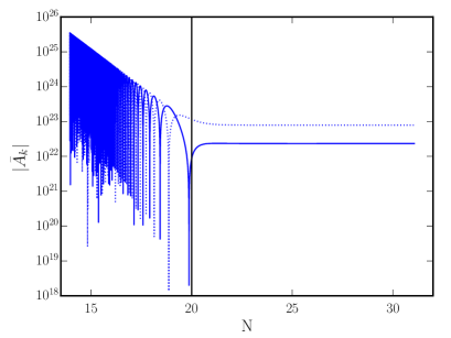
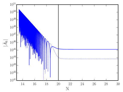
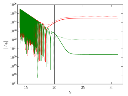
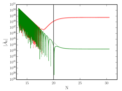
Figure 1: The evolution of the mode $\bar{A}_{k}^{\sigma}$ has been plotted as a function of e-folds $N$ for $n=1$ (on the left) and $n=2$ (on the right) for the wavenumber $k=0.002\,{\rm Mpc}^{-1}$ for the cases $\gamma=0$ (on top, in blue) and $\gamma=2$ (at the bottom, in red and green). We have plotted the absolute values of the real (solid lines) and imaginary (dashed lines) parts separately so that the oscillations are visible. The black vertical lines in each plot indicate the e-fold at which the modes leave the Hubble radius. Note that, around the time when the modes leave the Hubble radius, the $\sigma=-1$ mode (in red) is amplified when compared to the non-helical case, whereas the $\sigma=1$ mode (in green) is suppressed. Also, as expected, the amplification and suppression are more in the $n=2$ case than in the $n=1$ case.

At this stage, we should comment on the amplitude of the parity violating parameter $\gamma$ that we have worked with. As is well known, magnetic fields possess anisotropic stress. Such anisotropic stresses can act as a source for the primordial gravitational waves and boost their amplitude [41]. Since the strength of the helical modes are amplified more compared to the non-helical modes, one finds that they will in turn affect the amplitude of the tensor modes to a larger extent. The contribution of the helical magnetic fields to the primordial gravitational waves and the current upper bound on the tensor-to-scalar ratio impose constraints on a combination of the scale of inflation $H/M_{{}_{\rm Pl}}$ and the parameter $\xi$ (recall that, $\xi$ is related to $\gamma$ through the expression $\xi=-n\,\gamma$). We find that the effects of these helical fields on the primordial gravitational waves have been calculated explicitly for $n<0$ (in this context, see Ref. [41]), but not for the cases of our interest, i.e. $n=1$ and $n=2$. If we extrapolate the arguments for $n<0$ to our cases and use the current upper bound on the tensor-to-scalar ratio, viz. $r\lesssim 10^{-2}$, then we find that $\xi\lesssim 10$. We should add that, even if we vary $r$ or the quantity $H/M_{{}_{\rm Pl}}$ over a reasonably wide range, the upper limit on $\xi$ is not affected substantially. This is consistent with $\gamma=2$ that we have worked with here.

5.2 Evaluation of the three-point function

Before we go on to consider the cross-correlation of our interest, let us make a few clarifying remarks concerning the numerical evaluation of the inflationary two-point and three-point functions involving the scalar and the tensor perturbations. The inflationary correlation functions are formally expected to be evaluated at the end of inflation. However, it is well known that, during inflation, the amplitude of the scalar and the tensor perturbations freeze on super-Hubble scales (apart from some peculiar situations). This behavior makes it convenient for the numerical evaluation of the power spectra, since they can be evaluated soon after the modes leave the Hubble radius. Typically, the initial conditions are imposed when the modes are sufficiently inside the Hubble radius [say, when $k/(a\,H)\simeq 10^{2}$] and the power spectra are evaluated when the modes are sufficiently outside [say, when $k/(a\,H)\simeq 10^{-5}$]. As far as the three-point functions are concerned, apart from arriving at the modes, we also need to integrate over them from very early to late times. One can show that, due to the above-mentioned freezing of the amplitude of the perturbations, the super-Hubble contributions to the three-point functions are insignificant (in this context, see, for instance, Refs. [59, 60, 61]). Since the three-point function involves an arbitrary triangular configuration of wavevectors, to arrive at them, the initial conditions are imposed when the mode with the smallest of the wavenumbers is sufficiently inside the Hubble radius (say, at the e-fold $N_{i}$) and the integrals involved are evaluated until the mode with the largest of the wavenumbers is adequately outside (say, at $N_{s}$) [62, 63, 59, 60, 61].

There is yet another point to be attended to when evaluating the three-point functions numerically. All the modes will oscillate strongly in the sub-Hubble domain. Therefore, in order to evaluate the integrals involved, analytically, a small parameter, say, $\kappa$, is introduced to achieve an exponential cut-off and thereby regulate these oscillations [64]. Actually, such a regulation is essential to ensure the correct choice of the perturbative quantum vacuum [64, 65]. One eventually considers the vanishing limit of the parameter $\kappa$ to arrive at the final forms of the three-point functions. The regulator proves to be very convenient in the numerical efforts, as it can ensure the convergence of the integrals. But, a couple of exercises need to be carried out to identify an apt value for the cut-off parameter such that the resulting three-point function is ideally independent of the choice of $\kappa$, $N_{i}$ and $N_{s}$. We find that the above arguments for the scalar and the tensor perturbations can be applied to the cross-correlation of our interest for the $n=1$ case. However, the $n=2$ case poses a peculiar difficulty not often encountered in the three-point functions involving the scalars and the tensors, and needs to handled with care. We shall make use of the analytical expressions available in the non-helical case to check the accuracy of our numerical computations.

In order to identify suitable values of $\kappa$, $N_{i}$ and $N_{s}$, we shall evaluate the two contributions to the three-point function of our interest [described by the integrals (4.15)] in the equilateral limit for different combinations of these variables. Earlier, we had mentioned that we solve the differential equations involved [viz. Eqs. (5.2) and (5.4)] using the fifth order Runge-Kutta routine. We shall carry out the integrals (4.15) using the Boole’s rule [66]. We should add that, in our discussion hereafter, for convenience, we shall simply set the polarization tensor $\varepsilon^{\bm{k}}_{\sigma i}$ to unity. However, we shall include all the contributions due to the positive and negative helicity modes as well as the cross terms that arise. We shall first keep $N_{s}$ fixed and calculate the quantities for three different values of $N_{i}$ and varied $\kappa$. This helps us identify a suitable combination of $N_{i}$ and $\kappa$ for which the three-point function is insensitive to the choice of these variables. We shall then choose these values of $N_{i}$ and $\kappa$ and attempt to identify a suitable choice for $N_{s}$. The results of these exercises are plotted in Figs. 2 and 3 for both the non-helical and helical cases for $n=1$ as well as $n=2$. In Fig. 2, we have illustrated the dependence of the two contributions to the three-point function on the sub-Hubble cut-off parameter $\kappa$ for different choices of $N_{i}$. It is clear from the figure that, for instance, for $N_{i}$ corresponding to $k=300\,\sqrt{J^{\prime\prime}/J}$, the two contributions to the three-point function are largely independent of $\kappa$ around $\kappa=0.1$. Therefore, we shall work with these values.

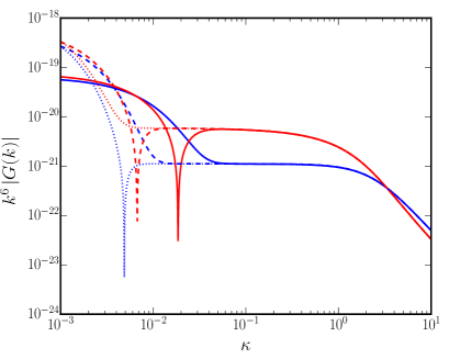
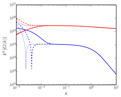
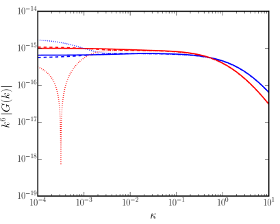
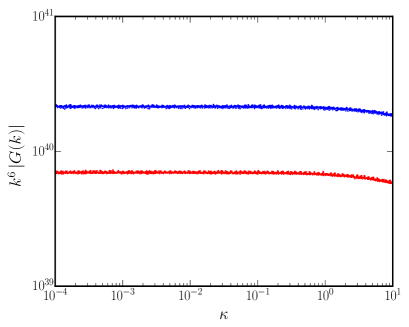
Figure 2: The amplitudes of the contributions to the three-point function arising from the first (in blue) and second (in red) integrals [cf. Eqs. (4.15)] have been plotted for the $n=1$ case (on the left) and the $n=2$ case (on the right) as functions of the cut-off parameter $\kappa$. We have plotted the results for three different choices of $N_{i}$ corresponding to $k=100\,\sqrt{J^{\prime\prime}/J}$ (as solid lines), $k=500\,\sqrt{J^{\prime\prime}/J}$ (as dashed lines) and $k=1000\,\sqrt{J^{\prime\prime}/J}$ (as dotted lines). Also, we have plotted them for the non-helical case (on top) as well as the helical case with $\gamma=2$ (at the bottom). Note that the two contributions to the three-point function have been multiplied with suitable powers of $k$. It should be clear from the above plots that, for the choice of $k=300\,\sqrt{J^{\prime\prime}/J}$, the resulting contributions are largely insensitive to $\kappa$ around $\kappa=0.1$. Because of this reason, we shall choose to evaluate the three-point function and the corresponding non-Gaussianity parameter (see the next section) for this choice of values. It is also useful to note from the final plot that the three-point function corresponding to $n=2$ in the helical case is largely unaffected by the value of the sub-Hubble cut-off parameter. As we shall see in the next figure, this occurs due to the fact that the dominant contribution to this three-point function arises from the super-Hubble domain.

Let us now turn to determining a suitable $N_{s}$. With $\kappa$ and $N_{i}$ fixed at the aforementioned values, in Fig. 3, we have plotted the two contributions as a function of $N_{s}$.

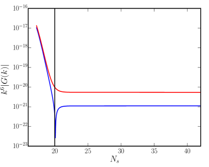
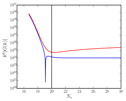
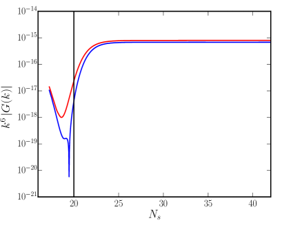
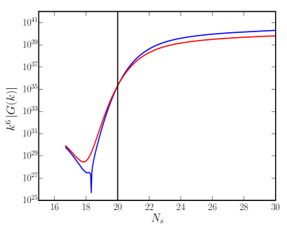
Figure 3: The amplitudes of the contributions to the three-point function arising from the first and the second integrals have been plotted for the $n=1$ and the $n=2$ cases as functions of $N_{s}$, with the same choice of colors as in the previous figure. Also, we have plotted the non-helical and the helical cases just as in the last figure. We have imposed the initial condition at an $N_{i}$ corresponding to $k=300\,\sqrt{J^{\prime\prime}/J}$, and we have set $\kappa=0.1$ in arriving at the above plots. We have plotted the results for a mode with the wavenumber $k=0.002\,{\rm Mpc}^{-1}$, which is often chosen as the pivot scale when comparing with the observations. The black vertical lines in the plots indicate the e-fold at which the mode leaves the Hubble radius. Note that, in the $n=1$ case, the amplitude of the two terms freeze soon after Hubble exit, which implies that the super-Hubble contributions to the three-point function are negligible. This is true in the corresponding helical case as well. When $n=2$, for the non-helical case, even though the first integral flattens out in the super-Hubble limit, the contribution due to the second integral continues to grow. This behavior has been encountered in analytical calculations and it can be attributed to the ${\rm ln}(-k\,\eta_{\rm e})$ term that arises in this case. It is also clear from the plots that the introduction of helicity considerably enhances the amplitude of the three-point functions. Moreover, the enhancement occurs around the time the mode leaves the Hubble radius. This is further accentuated by the super-Hubble contributions that are encountered in the $n=2$ case.

Note that, in the $n=1$ case, the results are independent of the choice $N_{s}$, provided we choose it corresponding to a time reasonably after Hubble exit. In contrast, when $n=2$, it is clear from the figure that there is a slow growth as a function of $N_{s}$. Such a behavior is peculiar to the model and the choices of the parameter involved. This growth is well known from the analytical calculations and, in the non-helical case, it can be shown to behave as ${\rm ln}\,(-\,k\,\eta_{\rm e})$ (in the equilateral limit we are focusing on), which is exactly the behavior we observe numerically [52, 67]. It is also clear from Fig. 3 that the introduction of helicity considerably enhances the amplitude of the three-point function in both the $n=1$ and $n=2$ cases. Moreover, it is evident that the enhancement occurs as the modes leave the Hubble radius, which is further accentuated in the $n=2$ case due to the super-Hubble contributions that arise. While the results will be independent of $N_{s}$ in the $n=1$ case, they will strongly depend on the parameter when $n=2$. Ideally, it would have been desirable to evaluate the three-point function when inflation ends at $60$ e-folds or so since the earliest time when, say, the largest scale had exited the Hubble radius. However, evolving the modes for this duration and evaluating the integrals introduce inaccuracies after about $30$ e-folds or so. Therefore, we shall evaluate the three-point function in the $n=2$ case for $N_{s}\sim 30$.

6 Amplitude and shape of the non-Gaussianity parameter

In this section, we shall introduce the dimensional non-Gaussianity parameter $b_{{}_{\rm NL}}$ which characterizes the amplitude and shape of the three-point function involving the helical magnetic field and the perturbations in the scalar field. We shall present the numerical results for $b_{{}_{\rm NL}}$ for the different cases we had discussed. In order to illustrate the accuracy of our numerical methods, we shall also compare our numerical results with the analytical results that are available in the non-helical case.

The amplitude of the non-Gaussianity in the local model for the scalar three-point function is usually parameterized in terms of a parameter $f_{{}_{\rm NL}}$ which, in this model, coincides with the bispectrum scaled by products of the power spectra. Here, we generalize that analogously to a non-Gaussianity parameter $b_{{}_{\rm NL}}$ which we define through the following relation:

$$\hat{B}_{i\,\bm{q}}(\eta)=\hat{B}_{i\,\bm{q}}^{({\rm G})}(\eta)+\frac{b_{{}_{\rm NL}}}{2\,M_{{}_{\rm Pl}}}\,\int\frac{{\rm d}^{3}\bm{p}}{(2\,\pi)^{3/2}}\,\hat{\delta\phi}_{\bm{q}-\bm{p}}(\eta)\,\hat{B}_{i\,{\bm{p}}}^{({\rm G})}(\eta),$$ (6.1)

where $\hat{B}_{i\,\bm{q}}$ is the Fourier mode of the actual magnetic field and $\hat{B}_{i\,\bm{q}}^{({\rm G})}$ indicates the Fourier mode of its Gaussian part, while, as usual, $\hat{\delta\phi}_{\bm{q}-\bm{p}}$ refers to Fourier mode of the perturbation in the scalar field which has already been assumed to be Gaussian. Upon using Wick’s theorem to calculate the three-point function of our interest, we find that we can express the parameter $b_{{}_{\rm NL}}$ as

$$b_{{}_{\rm NL}}\left(\bm{k_{1}},\bm{k_{2}},\bm{k_{3}}\right) = \frac{1}{16\,\pi^{5}}\,\frac{J^{2}(\eta_{\rm e})}{a^{2}({\eta_{\rm e}})}\,\biggl{[}k_{1}^{3}\,k_{2}^{3}\,k_{3}^{3}\,G_{\delta\phi BB}(\bm{k_{1}},\bm{k_{2}},\bm{k_{3}})\biggr{]}$$ (6.2)

$$\times\,\biggl{\{}{\cal P}_{\delta\phi}(k_{1})\left[k_{3}^{3}\,{\mathcal{P}}_{{}_{\rm B}}(k_{2})+k_{2}^{3}\,{\mathcal{P}}_{{}_{\rm B}}(k_{3})\right]\biggr{\}}^{-1}.$$

In this expression, ${\mathcal{P}}_{{}_{\rm B}}(k)$ denotes the power spectrum of the magnetic field that we have discussed earlier, while ${\cal P}_{\delta\phi}(k)$ denotes the power spectrum of the perturbations in the scalar field that is defined as

$${\cal P}_{\delta\phi}(k)=\frac{k^{3}}{2\,\pi^{2}\,M_{{}_{\rm Pl}}^{2}}\,|\,f_{k}(\eta_{\rm e})|^{2},$$ (6.3)

with the right hand side to be evaluated as $\eta_{\rm e}\to 0$.

In Fig. 4, we have plotted the numerical results for the non-Gaussianity parameter $b_{{}_{\rm NL}}$ (for an arbitrary triangular configuration of wavenumbers, in this context, see Ref. [67]) for the cases of $n=1$ and $n=2$ when $\gamma=0$ and $\gamma=2$. We have also plotted the analytical results available for $n=1$ and $n=2$ in the non-helical case, to illustrate the extent of accuracy of our numerical methods.

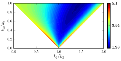
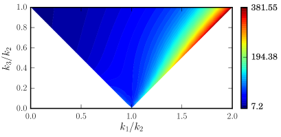
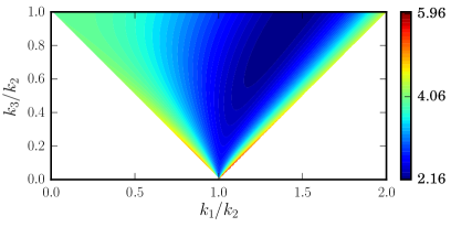
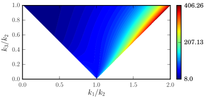
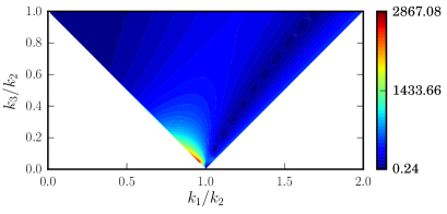
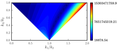
Figure 4: The non-Gaussianity parameter $b_{{}_{\rm NL}}$ has been plotted for the non-helical case obtained numerically (top row), analytically (middle row), and the helical case arrived at numerically (third row of plots) for the cases of $n=1$ (on the left) and $n=2$ (on the right). For reasons we have discussed, in the $n=2$ case, we have evaluated the non-Gaussianity parameter corresponding to $N_{s}\sim 30$. From the first and second rows, we find that the analytical and numerical results match up to $5$–$10\%$. It is evident from the third row of plots that the helical term substantially boosts the value of $b_{{}_{\rm NL}}$ for both the $n=1$ and $n=2$ cases, with the amplification being larger for $n=2$.

On comparing the results in the non-helical case for $n=1$ and $n=2$, we find that the analytical and numerical results match up to about $5$–$10\%$. Recall that we have been working with $\gamma=2$. Even for such a relatively small value of $\gamma$, we find that the introduction of helicity considerably amplifies non-Gaussianities.

7 Summary

The generation and evolution of primordial magnetic fields has been studied extensively in the context of inflation. By introducing a non-minimal coupling term in the standard electromagnetic action, it has been possible to obtain scale invariant magnetic fields of the requisite amplitude to be in conformity with observations. It has also been realized that adding a parity violating term to the electromagnetic action results in the production of helical magnetic fields, which can have significant observational imprints [43, 44, 45, 30]. Specifically, helicity considerably boosts the amplitude of the power spectrum of the magnetic field.

The non-Gaussian signatures generated via cross-correlations between the primordial magnetic fields and the perturbations in a scalar field can provide additional constraints to characterize the magnetic fields. These non-Gaussianities, at the level of three-point functions, have been examined earlier in the non-helical case [49, 50, 51, 52]. In this work, we numerically evaluate the three-point functions involving primordial helical magnetic fields and the perturbations in a scalar field. Since the introduction of the helical term in the action amplifies the strength of the magnetic field, it can also be expected to lead to larger non-Gaussianities. We find that even with a small value of the parameter quantifying the extent of helicity, there is a substantial enhancement in the non-Gaussianity parameter $b_{{}_{\rm NL}}$. It would be interesting to explore related observational consequences, and possibly arrive at constraints on the mechanisms that could lead to the generation of the helical magnetic fields (in this context, see Ref. [68]). Another important aspect would be to investigate into the behavior of the three-point functions involving the helical magnetic fields and the curvature perturbation [50, 52]. Importantly, in such a case, one may encounter additional terms arising in the action describing the interaction term. Also, while the magnitude of $b_{{}_{\rm NL}}$ in, say, slow roll inflation, may not differ substantially from the case we have examined, considering the curvature perturbation can provide us with additional parameters (viz. the slow roll parameters) to more effectively constrain the non-Gaussianities generated. We are presently working on these issues.

References

- [1] A. Neronov and I. Vovk, Evidence for strong extragalactic magnetic fields from Fermi observations of TeV blazars, Science 328 (2010) 73–75, [arXiv:1006.3504].
- [2] F. Tavecchio et al., The intergalactic magnetic field constrained by Fermi/LAT observations of the TeV blazar 1ES 0229+200, Mon. Not. Roy. Astron. Soc. 406 (2010) L70–L74, [arXiv:1004.1329].
- [3] C. D. Dermer, M. Cavadini, S. Razzaque, J. D. Finke, and B. Lott, Time Delay of Cascade Radiation for TeV Blazars and the Measurement of the Intergalactic Magnetic Field, Astrophys. J. 733 (2011) L21, [arXiv:1011.6660].
- [4] I. Vovk, A. M. Taylor, D. Semikoz, and A. Neronov, Fermi/LAT observations of 1ES 0229+200: implications for extragalactic magnetic fields and background light, Astrophys. J. 747 (2012) L14, [arXiv:1112.2534].
- [5] F. Tavecchio, G. Ghisellini, G. Bonnoli, and L. Foschini, Extreme TeV blazars and the intergalactic magnetic field, Mon. Not. Roy. Astron. Soc. 414 (2011) 3566, [arXiv:1009.1048].
- [6] K. Dolag, M. Kachelriess, S. Ostapchenko, and R. Tomas, Lower limit on the strength and filling factor of extragalactic magnetic fields, Astrophys. J. 727 (2011) L4, [arXiv:1009.1782].
- [7] A. M. Taylor, I. Vovk, and A. Neronov, Extragalactic magnetic fields constraints from simultaneous GeV-TeV observations of blazars, Astron. Astrophys. 529 (2011) A144, [arXiv:1101.0932].
- [8] K. Takahashi, M. Mori, K. Ichiki, and S. Inoue, Lower Bounds on Intergalactic Magnetic Fields from Simultaneously Observed GeV-TeV Light Curves of the Blazar Mrk 501, Astrophys. J. 744 (2012) L7, [arXiv:1103.3835].
- [9] H. Huan, T. Weisgarber, T. Arlen, and S. P. Wakely, A New Model for Gamma-Ray Cascades in Extragalactic Magnetic Fields, Astrophys. J. 735 (2011) L28, [arXiv:1106.1218].
- [10] J. D. Finke, L. C. Reyes, M. Georganopoulos, K. Reynolds, M. Ajello, S. J. Fegan, and K. McCann, Constraints on the Intergalactic Magnetic Field with Gamma-Ray Observations of Blazars, Astrophys. J. 814 (2015), no. 1 20, [arXiv:1510.02485].
- [11] D. Grasso and H. R. Rubinstein, Magnetic fields in the early universe, Phys. Rept. 348 (2001) 163–266, [astro-ph/0009061].
- [12] L. M. Widrow, Origin of Galactic and Extragalactic Magnetic Fields, Rev. Mod. Phys. 74 (2002) 775–823, [astro-ph/0207240].
- [13] A. Kandus, K. E. Kunze, and C. G. Tsagas, Primordial magnetogenesis, Phys. Rept. 505 (2011) 1–58, [arXiv:1007.3891].
- [14] L. M. Widrow, D. Ryu, D. R. Schleicher, K. Subramanian, C. G. Tsagas, et al., The First Magnetic Fields, Space Sci. Rev. 166 (2012) 37–70, [arXiv:1109.4052].
- [15] R. Durrer and A. Neronov, Cosmological Magnetic Fields: Their Generation, Evolution and Observation, Astron. Astrophys. Rev. 21 (2013) 62, [arXiv:1303.7121].
- [16] K. Subramanian, The origin, evolution and signatures of primordial magnetic fields, Rept. Prog. Phys. 79 (2016), no. 7 076901, [arXiv:1504.02311].
- [17] Planck Collaboration, P. Ade et al., Planck 2015 results. XIX. Constraints on primordial magnetic fields, arXiv:1502.01594.
- [18] POLARBEAR Collaboration, P. A. R. Ade et al., POLARBEAR Constraints on Cosmic Birefringence and Primordial Magnetic Fields, Phys. Rev. D92 (2015) 123509, [arXiv:1509.02461].
- [19] K. Subramanian, Magnetic fields in the early universe, Astron. Nachr. 331 (2010) 110–120, [arXiv:0911.4771].
- [20] M. Giovannini, Probing large-scale magnetism with the Cosmic Microwave Background, Class. Quant. Grav. 35 (2018), no. 8 084003, [arXiv:1712.07598].
- [21] M. S. Turner and L. M. Widrow, Inflation Produced, Large Scale Magnetic Fields, Phys. Rev. D37 (1988) 2743.
- [22] B. Ratra, Cosmological ’seed’ magnetic field from inflation, Astrophys. J. 391 (1992) L1–L4.
- [23] K. Bamba and J. Yokoyama, Large scale magnetic fields from inflation in dilaton electromagnetism, Phys. Rev. D69 (2004) 043507, [astro-ph/0310824].
- [24] K. Bamba and M. Sasaki, Large-scale magnetic fields in the inflationary universe, JCAP 0702 (2007) 030, [astro-ph/0611701].
- [25] V. Demozzi, V. Mukhanov, and H. Rubinstein, Magnetic fields from inflation?, JCAP 0908 (2009) 025, [arXiv:0907.1030].
- [26] J. Martin and J. Yokoyama, Generation of Large-Scale Magnetic Fields in Single-Field Inflation, JCAP 0801 (2008) 025, [arXiv:0711.4307].
- [27] L. Campanelli, Helical Magnetic Fields from Inflation, Int. J. Mod. Phys. D18 (2009) 1395–1411, [arXiv:0805.0575].
- [28] S. Kanno, J. Soda, and M.-a. Watanabe, Cosmological Magnetic Fields from Inflation and Backreaction, JCAP 0912 (2009) 009, [arXiv:0908.3509].
- [29] F. R. Urban, On inflating magnetic fields, and the backreactions thereof, JCAP 1112 (2011) 012, [arXiv:1111.1006].
- [30] R. Durrer, L. Hollenstein, and R. K. Jain, Can slow roll inflation induce relevant helical magnetic fields?, JCAP 1103 (2011) 037, [arXiv:1005.5322].
- [31] C. T. Byrnes, L. Hollenstein, R. K. Jain, and F. R. Urban, Resonant magnetic fields from inflation, JCAP 1203 (2012) 009, [arXiv:1111.2030].
- [32] R. K. Jain, R. Durrer, and L. Hollenstein, Generation of helical magnetic fields from inflation, J.Phys.Conf.Ser. 484 (2014) 012062, [arXiv:1204.2409].
- [33] T. Kahniashvili, A. Brandenburg, L. Campanelli, B. Ratra, and A. G. Tevzadze, Evolution of inflation-generated magnetic field through phase transitions, Phys.Rev. D86 (2012) 103005, [arXiv:1206.2428].
- [34] S.-L. Cheng, W. Lee, and K.-W. Ng, Inflationary dilaton-axion magnetogenesis, arXiv:1409.2656.
- [35] K. Bamba, Generation of large-scale magnetic fields, non-Gaussianity, and primordial gravitational waves in inflationary cosmology, Phys. Rev. D91 (2015) 043509, [arXiv:1411.4335].
- [36] T. Fujita, R. Namba, Y. Tada, N. Takeda, and H. Tashiro, Consistent generation of magnetic fields in axion inflation models, JCAP 1505 (2015), no. 05 054, [arXiv:1503.05802].
- [37] L. Campanelli, Lorentz-violating inflationary magnetogenesis, Eur. Phys. J. C75 (2015), no. 6 278, [arXiv:1503.07415].
- [38] T. Fujita and R. Namba, Pre-reheating Magnetogenesis in the Kinetic Coupling Model, arXiv:1602.05673.
- [39] C. G. Tsagas, Causality, initial conditions, and inflationary magnetogenesis, Phys. Rev. D93 (2016), no. 10 103529, [arXiv:1603.05209].
- [40] R. Sharma, S. Jagannathan, T. R. Seshadri, and K. Subramanian, Challenges in Inflationary Magnetogenesis: Constraints from Strong Coupling, Backreaction and the Schwinger Effect, Phys. Rev. D96 (2017), no. 8 083511, [arXiv:1708.08119].
- [41] C. Caprini and L. Sorbo, Adding helicity to inflationary magnetogenesis, JCAP 1410 (2014), no. 10 056, [arXiv:1407.2809].
- [42] R. Sharma, K. Subramanian, and T. R. Seshadri, Generation of helical magnetic field in a viable scenario of inflationary magnetogenesis, Phys. Rev. D97 (2018), no. 8 083503, [arXiv:1802.04847].
- [43] C. Caprini, R. Durrer, and T. Kahniashvili, The Cosmic microwave background and helical magnetic fields: The Tensor mode, Phys. Rev. D69 (2004) 063006, [astro-ph/0304556].
- [44] M. Ballardini, F. Finelli, and D. Paoletti, CMB anisotropies generated by a stochastic background of primordial magnetic fields with non-zero helicity, JCAP 1510 (2015), no. 10 031, [arXiv:1412.1836].
- [45] N. Seto and A. Taruya, Polarization analysis of gravitational-wave backgrounds from the correlation signals of ground-based interferometers: Measuring a circular-polarization mode, Phys. Rev. D77 (2008) 103001, [arXiv:0801.4185].
- [46] A. Brandenburg and K. Subramanian, Astrophysical magnetic fields and nonlinear dynamo theory, Phys. Rept. 417 (2005) 1–209, [astro-ph/0405052].
- [47] R. Banerjee and K. Jedamzik, The Evolution of cosmic magnetic fields: From the very early universe, to recombination, to the present, Phys. Rev. D70 (2004) 123003, [astro-ph/0410032].
- [48] L. Campanelli, Evolution of Magnetic Fields in Freely Decaying Magnetohydrodynamic Turbulence, Phys. Rev. Lett. 98 (2007) 251302, [arXiv:0705.2308].
- [49] R. R. Caldwell, L. Motta, and M. Kamionkowski, Correlation of inflation-produced magnetic fields with scalar fluctuations, Phys. Rev. D84 (2011) 123525, [arXiv:1109.4415].
- [50] L. Motta and R. R. Caldwell, Non-Gaussian features of primordial magnetic fields in power-law inflation, Phys. Rev. D85 (2012) 103532, [arXiv:1203.1033].
- [51] R. K. Jain and M. S. Sloth, Consistency relation for cosmic magnetic fields, Phys. Rev. D86 (2012) 123528, [arXiv:1207.4187].
- [52] R. K. Jain and M. S. Sloth, On the non-Gaussian correlation of the primordial curvature perturbation with vector fields, JCAP 1302 (2013) 003, [arXiv:1210.3461].
- [53] M. M. Anber and L. Sorbo, N-flationary magnetic fields, JCAP 0610 (2006) 018, [astro-ph/0606534].
- [54] “NIST Digital Library of Mathematical Functions.” http://dlmf.nist.gov/, Release 1.0.13 of 2016-09-16. F. W. J. Olver, A. B. Olde Daalhuis, D. W. Lozier, B. I. Schneider, R. F. Boisvert, C. W. Clark, B. R. Miller and B. V. Saunders, eds.
- [55] I. S. Gradshteyn and I. M. Ryzhik, Table of Integrals, Series, and Products. Academic Press, New York, 7th ed., 2007.
- [56] M. Abramowitz and I. A. Stegun, Handbook of Mathematical Functions. Dover, New York, USA, 2001.
- [57] N. Bartolo, S. Matarrese, M. Peloso, and M. Shiraishi, Parity-violating CMB correlators with non-decaying statistical anisotropy, JCAP 1507 (2015), no. 07 039, [arXiv:1505.02193].
- [58] N. Bartolo, S. Matarrese, M. Peloso, and M. Shiraishi, Parity-violating and anisotropic correlations in pseudoscalar inflation, JCAP 1501 (2015), no. 01 027, [arXiv:1411.2521].
- [59] D. K. Hazra, L. Sriramkumar, and J. Martin, BINGO: A code for the efficient computation of the scalar bi-spectrum, JCAP 1305 (2013) 026, [arXiv:1201.0926].
- [60] V. Sreenath, R. Tibrewala, and L. Sriramkumar, Numerical evaluation of the three-point scalar-tensor cross-correlations and the tensor bi-spectrum, JCAP 1312 (2013) 037, [arXiv:1309.7169].
- [61] V. Sreenath, D. K. Hazra, and L. Sriramkumar, On the scalar consistency relation away from slow roll, JCAP 1502 (2015), no. 02 029, [arXiv:1410.0252].
- [62] X. Chen, R. Easther, and E. A. Lim, Large Non-Gaussianities in Single Field Inflation, JCAP 0706 (2007) 023, [astro-ph/0611645].
- [63] X. Chen, R. Easther, and E. A. Lim, Generation and Characterization of Large Non-Gaussianities in Single Field Inflation, JCAP 0804 (2008) 010, [arXiv:0801.3295].
- [64] J. M. Maldacena, Non-Gaussian features of primordial fluctuations in single field inflationary models, JHEP 05 (2003) 013, [astro-ph/0210603].
- [65] D. Seery and J. E. Lidsey, Primordial non-Gaussianities in single field inflation, JCAP 0506 (2005) 003, [astro-ph/0503692].
- [66] W. H. Press, S. A. Teukolsky, W. T. Vetterling, and B. P. Flannery, Numerical Recipes 3rd Edition: The Art of Scientific Computing. Cambridge University Press, New York, NY, USA, 3 ed., 2007.
- [67] D. Chowdhury, L. Sriramkumar, and M. Kamionkowski, Cross-correlations between scalar perturbations and magnetic fields in bouncing universes, arXiv:1807.05530.
- [68] K. E. Kunze, CMB and matter power spectra from cross correlations of primordial curvature and magnetic fields, Phys. Rev. D87 (2013), no. 10 103005, [arXiv:1301.6105].