Braneworld inflation with effective $\alpha$-attractor potential

Abstract

In this paper, we study inflation in $\alpha$-attractor framework with exponential potential in the RS braneworlds where high energy corrections to the Friedmann equation facilitate slow roll. In this scenario, we numerically investigate the inflationary parameters and show that the high energy brane corrections have significant effect on the parameter $\alpha$, namely, the lower values of the parameter are preferred by observation in this limit. The latter substantially reduces the tensor to scalar ratio of perturbations making the RS brane world inflation compatible with observation. We also point out that the sub-Planckian values of the field displacement can be achieved by suitably constraining the brane tension.

I Introduction

In the standard framework, a slowly rolling scalar field a la a shallow field potential may account for inflationLinde1 . Slow roll along a steep potential is also possible due to Hubble damping caused by high energy brane corrections. Indeed, in brane world scenario, our four dimensional space-time dubbed brane is supposed to be embedded in a higher dimensional bulk brane ; Randall:1999vf such that the Einstein equations on the brane are modified. The corresponding Friedmann equation includes an extra termbranecor1 ; branecor2 , quadratic in density which facilitates slow roll in high energy regime at early times even in case of a steep potentialfrictionbrane1 ; frictionbrane2 ; Gong:2000en ; Apostolopoulos:2005ff . Thus, brane world scenario allows steep potential to support inflation Sahni:2001qp ; Sami:2004xk ; Copeland:2000hn which is not possible in standard case.
In the standard cosmology, an exponential potentialexpon does not give viable inflationary and post inflationary behavior. The situation changes significantly in the brane-world case Sahni:2001qp ; Sami:2004xk ; Copeland:2000hn . However, the steep braneworld inflation gives a ratio of tensor to scalar perturbation, $r$, around $0.4$ for 60 $e$-$folds$ of inflation Copeland:2000hn ; Tsujikawa:2003zd which is not tenable observationallyplanck ; bicep ; Ade:2018gkx ; Akrami:2018odb . Similar problem in the standard cosmology can successfully be addressed in the $\alpha$-attractor scenarioLinde:2016uec ; Dimopoulos:2017zvq ; Dimopoulos:2017tud ; Akrami:2017cir ; Shahalam:2018rby ; Shahalam:2016juu . In this framework, the kinetic term in the Lagrangian has a specif non canonical form. Canonicalization of such term gives rise to some flat regions or plateaus in the potentialLinde:2016uec ; Dimopoulos:2017zvq ; Dimopoulos:2017tud ; Akrami:2017cir which are suitable for the study of inflation favored by observational dataplanck ; bicep ; Ade:2018gkx ; Akrami:2018odb . This feature can also be suitable for the study of late time behavior, namely, quintessence Dimopoulos:2017zvq ; Dimopoulos:2017tud ; Garcia-Garcia:2018hlc ; Peebles:1998qn ; samiDE ; Hossain:2014zma ; Mishra:2017ehw ; Sami:2004ic ; Akrami:2017cir ; Rubio:2017gty .

It should be mention here that a super-Planckian displacement of the scalar field may spoil the flatness of quintessential region of the potential and may generate an unwanted fifth force problemDimopoulos:2017zvq ; Dimopoulos:2017tud ; Akrami:2017cir ; xxx . On the other hand, it is impossible to evolve to quintessence starting from the inflationary region without invoking super-Planckian values of the field and not making the potential too curve during inflationDimopoulos:2002hm . The $\alpha$-attractor solves this problem, namely, the canonicalization of the potential makes it possible for the canonical scalar field to have a super-Planckian excursion while keeping its non-canonical counter part under sub-Planckian.
In view of the aforesaid, we are led to consider the $\alpha$ attractor construct in the framework of RS brane worldsRandall:1999vf which might give new insights related to the sub-Planckian nature of non-canonical field

The structure of this paper is as follows. In section (II), we discuss how we obtain our effective $\alpha$-attractor potential and suggest some approximations to check for analytical behavior. In section (III), we put the effective potential on brane and perform a full numerical study of different parameters related to inflation. Numerical analysis is done because of complexity in solving the problem analytically. In this section, we also show some important features our model exhibits. Next, in section(IV) we show some approximated analytical results for our model. Next, in section (V), we compare our results with current observational bounds and with the results obtained, we constrain our different model parameters especially the parameter $\alpha$. Next, in section (VI) we briefly discuss the late time behavior followed by conclusions in section (VII).

II The effective $\alpha$-attractor model

Considering the formal $\alpha$-attractor Lagrangian density with an exponential potential in 4-dimensional space-timeLinde:2016uec ; Dimopoulos:2017zvq ; Dimopoulos:2017tud ; Akrami:2017cir

$$\mathcal{L}=\frac{\frac{1}{2}\left(\partial\phi\right)^{2}}{\left(1-\frac{\phi^{2}}{6\alpha m_{p}^{2}}\right)^{2}}+V_{0}e^{-\kappa\phi/m_{p}},$$ (1)

where $\alpha>0$ is a parameter featuring a pole in the kinetic energy, $m_{p}=\frac{1}{\sqrt{8\pi G}}$, is the 4-dimensional reduced Planck mass, $G$ is the Newton’s constant, $\kappa$ is the parameter determining the steepness of the potential, $V_{0}$ is a constant with the dimension of energy density. The modulus value of $\phi$ will remain less than $\sqrt{6\alpha}\,\ m_{p}$ for any finite value of $\alpha$ because the kinetic energy becomes singular at this value. This allows the scalar field to remain under sub-Planckian values as long as $\alpha\lesssim 1/6$. The same theory cab be described in terms of a canonicalized inflaton field $\varphi$ related to the non-canonical scalar field $\phi$ via the transformation

$$\phi=\sqrt{6\alpha}\hskip 1.99168ptm_{p}\tanh(\frac{\varphi}{\sqrt{6\alpha}m_{p}}).$$ (2)

From equation(2), it is clear the canonical field $\varphi$ can take any value, keeping the non-canonical $\phi$ sub-Planckian. By this transformation the potential given in equation(1) is described now in terms of the canonical field of the form

$$V(\varphi)=V_{0}e^{-\kappa\sqrt{6\alpha}\hskip 1.99168pt\tanh(\frac{\varphi}{\sqrt{6\alpha}m_{p}})}.$$ (3)

This potential corresponds two plateaus, see Fig. 1. The inflationary regime is featured by a plateau corresponds to $\phi\rightarrow-\sqrt{6\alpha}\,\ m_{p}$, or equivalently by $\varphi\rightarrow-\infty$, the other plateau is featured by $\phi\rightarrow\sqrt{6\alpha}\,\ m_{p}$ or equivalently by $\varphi\rightarrow\infty$, featuring quintessence. For the inflationary limit potential(3) becomes

Figure 1: potential of $\alpha$-attractor after canonicalization (3)
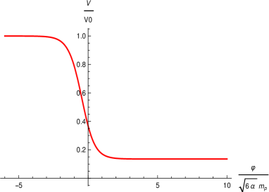
( $n$ is taken 1)

$$V(\varphi)=M^{4}\exp\left(-2ne^{\frac{2\sqrt{8\pi}}{\sqrt{6\alpha}\hskip 1.99168ptM_{Pl}}\varphi}\right)$$ (4)

where $M^{4}=V_{0}e^{\kappa\sqrt{6\alpha}}$, is a constant representing the energy scale for inflation, $M$ has dimension of mass, $M_{Pl}\equiv m_{p}\sqrt{8\pi}$ is the 4-dimensional Planck mass and $n\equiv\kappa\sqrt{6\alpha}$

III The effective $\alpha$-attractor potential in braneworld scenario

We place our effective potential on the Randall Sundrum II(RSII) braneRandall:1999vf to study the inflationary scenario. The matter fields are confined to the brane only for RSII model, so our scalar field will remain on the brane only. For a flat Friedmann-Lemaître-Robertson-Walker-Walker(FLRW) background on the brane with zero 4-dimensional cosmological constant, the Friedman equation becomes branecor1 ; Sahni:2001qp ; Sami:2004xk ; Tsujikawa:2003zd

$$H^{2}\equiv\left(\frac{\dot{a}}{a}\right)^{2}=\frac{8\pi}{3M_{Pl}^{2}}\rho\left(1+\frac{\rho}{2\lambda}\right),$$ (5)

where $a$ is the scale factor, $H$ is the Hubble parameter, $\rho$ is energy density of matter field on the brane, $\lambda$ is 3-brane tension relating the 4-d Planck mass, $M_{Pl}$ with 5-d Planck mass $M_{5}$ via

$$\lambda=\frac{3}{4\pi}\frac{{M_{5}}^{6}}{{M_{Pl}}^{2}}.$$ (6)

For high energies, $\rho^{2}$ term become significant and plays a crucial role in the dynamics of the scalar field, hence of the universe. The scalar field or the inflaton field $\varphi$, confined on the brane satisfies the Klein-Gordon equation

$$\ddot{\varphi}+3H\dot{\varphi}+V^{\prime}(\varphi)=0.$$ (7)

$V(\varphi)$ is the potential driving the inflation. The prime denotes a derivative with respect to $\varphi$ . The presence of quadratic term $\rho^{2}$ enhances the value of Hubble parameter (5) and hereby gives extra friction to the scalar field (7) and makes its evolution slower. Combining Eqs. (5) and (7) one gets the evolution equationfrictionbrane1 ; Tsujikawa:2003zd

$$\frac{\ddot{a}}{a}=\frac{8\pi}{3M_{Pl}^{2}}\left[(V-\dot{\varphi}^{2})+\frac{\dot{\varphi}^{2}+2V}{8\lambda}\left(2V-5\dot{\varphi}^{2}\right)\right]$$ (8)

The inflationary condition $\ddot{a}>0$, is reduced to standard form $V>\dot{\varphi}^{2}$   for   $\frac{\dot{\varphi}^{2}+2V}{8\lambda}\ll 1$. In the high energy scenario, the condition becomes $2V>5\dot{\varphi}^{2}$. This condition may used for characterizing end of inflation Tsujikawa:2003zd , $2V(\varphi_{end})\simeq 5\dot{\varphi}_{end}^{2}$ . Using the slow roll approximation ($V\gg\dot{\varphi}^{2}$ , $\frac{\ddot{\varphi}}{3H\dot{\varphi}}\ll 1$) we can write Eqs. (5) and (7) respectively as

$$H^{2}=\frac{8\pi}{3M_{Pl}^{2}}V\left(1+\frac{V}{2\lambda}\right)$$ (9)

and (10)

$$3H\dot{\varphi}+V^{\prime}(\varphi)=0.$$

These two Eqs. (9-10) make the condition for inflation end to be

$$\frac{V^{3}(\varphi_{end})}{V^{\prime 2}(\varphi_{end})}\simeq\frac{5\hskip 1.99168pt\lambda\hskip 1.99168ptM_{Pl}^{2}}{24\pi}.$$ (11)

The amplitude of scalar and tensor perturbation in RSII inflationary scenario are given asfrictionbrane1 ; Tsujikawa:2003zd ; Langlois:2000ns ; Dinda:2014zta

$$A_{S}^{2} = \left.\frac{512}{75M_{Pl}^{6}}\frac{V^{3}}{V^{\prime 2}}\left(1+\frac{V}{2\lambda}\right)^{3}\right|_{k=aH},$$ (12)

$$A_{T}^{2} = \left.\frac{4}{25\pi}\frac{H^{2}}{M_{Pl}^{2}}F^{2}(x)\right|_{k=aH},$$ (13)

where

$$x = HM_{Pl}\sqrt{3/\left(4\pi\lambda\right)}\,\ \simeq\sqrt{\frac{2V}{\lambda}(1+\frac{V}{2\lambda})},$$ (14)

$$F(x) = \left[\sqrt{1+x^{2}}-x^{2}\sinh^{-1}(1/x)\right]^{-1/2}.$$ (15)

The ’$\simeq$’ is used under slow-roll approximation. Amplitudes $A_{S}$ and $A_{T}$ are evaluated at horizon exit, $k=aH$, with $k$ being comoving wave number. The two slow roll parameters on the brane are given by

$$\epsilon \equiv \frac{M_{Pl}^{2}}{16\pi}\left(\frac{V^{\prime}}{V}\right)^{2}\frac{1+\frac{V}{\lambda}}{\left(1+\frac{V}{2\lambda}\right)^{2}},$$ (16)

$$\eta \equiv \frac{M_{Pl}^{2}}{8\pi}\frac{V^{\prime\prime}}{V}\frac{1}{1+\frac{V}{2\lambda}}.$$ (17)

which indicates that in high energy regime($V/\lambda\gg 1$), slow roll is possible even if the potential is steep. The spectral indices of scalar and tensor perturbations are

$$n_{S}-1 \equiv \left.\frac{d\ln{A_{S}}^{2}}{d\ln{k}}\right|_{k=aH},$$ (18)

$$n_{T} \equiv \left.\frac{d\ln{A_{T}}^{2}}{d\ln{k}}\right|_{k=aH}.$$ (19)

Under slow-roll conditions, we get

$$n_{S}=1-6\epsilon+2\eta.$$ (20)

The number of $e$ folds during inflation is given by $\int_{t_{*}}^{t_{end}}Hdt$ , which under slow-roll condition can be written as

$$N\simeq-\frac{8\pi}{M_{Pl}^{2}}\int_{\varphi_{*}}^{\phi_{end}}\frac{V}{V^{\prime}}\left(1+\frac{V}{2\lambda}\right)d\phi,$$ (21)

where $*$ denotes the value at the horizon exit. We define the ratio of tensor-to-scalar perturbation $r$ as Tsujikawa:2003zd

$$r\equiv 16\left(\frac{A_{T}^{2}}{A_{S}^{2}}\right).$$ (22)

In the high energy limit $V/\lambda\gg 1$ , one finds from Eq. (15) $F^{2}\simeq\frac{3V}{2\lambda}$, this together with the slow roll approximation ($\rho\sim V$), and using Eqs. (9), (12), and (13) we get,

$$r = \frac{M_{Pl}^{2}}{\pi}\left(\frac{V^{\prime}}{V}\right)^{2}\frac{1}{\left(1+V/2\lambda\right)^{2}}F^{2}$$ (23)

$$= \frac{3M_{Pl}^{2}}{2\pi}\left(\frac{V^{\prime}}{V}\right)^{2}\frac{V/\lambda}{\left(1+V/2\lambda\right)^{2}}\simeq 24\epsilon.$$

One can easily show that in the low energy limit($V/\lambda\ll 1$)$,\,\ r=16\epsilon$, which is the standard expression.

To study inflation, we start with the potential (4). The condition for inflation end (11) gives

$$\frac{3\alpha M^{4}M_{Pl}^{2}}{64\pi n^{2}}\exp\left[-\frac{8\sqrt{\frac{\pi}{3}}\hskip 1.99168pt\varphi_{end}}{\sqrt{\alpha}M_{Pl}}-2ne^{\frac{4\sqrt{\frac{\pi}{3}}\hskip 1.99168pt\varphi_{end}}{\sqrt{\alpha}M_{Pl}}}\right]$$ (24)

$$\simeq 5\frac{\lambda M_{Pl}^{2}}{24\pi}$$

The total number of $e$-foldings of inflation is given by (21) for high energy limit $(\frac{V}{\lambda}\gg 1$)

$$N\simeq\int_{\varphi_{*}}^{\varphi_{end}}\frac{\sqrt{3\pi}\sqrt{\alpha}M^{4}}{2n\lambda M_{Pl}}\exp\left[-\frac{4\sqrt{\frac{\pi}{3}}\hskip 1.99168pt\varphi}{\sqrt{\alpha}M_{Pl}}-2ne^{\frac{4\sqrt{\frac{\pi}{3}}\hskip 1.99168pt\varphi}{\sqrt{\alpha}M_{Pl}}}\right]d\varphi$$

(25)

The two slow roll parameters in the high energy limit become

$$\epsilon \simeq \frac{16n^{2}\lambda}{3\alpha M^{4}}\exp\left[\frac{8\sqrt{\frac{\pi}{3}}\hskip 1.99168pt\varphi}{\sqrt{\alpha}M_{Pl}}+2ne^{\frac{4\sqrt{\frac{\pi}{3}}\hskip 1.99168pt\varphi}{\sqrt{\alpha}M_{Pl}}}\right].$$ (26)

$$\eta \simeq \frac{8n\lambda}{3\alpha M^{4}}\left(2ne^{\frac{4\sqrt{\frac{\pi}{3}}\hskip 1.99168pt\varphi}{\sqrt{\alpha}M_{Pl}}}-1\right)\exp\left[\frac{4\sqrt{\frac{\pi}{3}}\hskip 1.99168pt\varphi}{\sqrt{\alpha}M_{Pl}}+2ne^{\frac{4\sqrt{\frac{\pi}{3}}\hskip 1.99168pt\varphi}{\sqrt{\alpha}M_{Pl}}}\right]$$

(27)

We do solve Eqs. (24) and (25) numerically and using (26) and (27), we compute $r$ and $n_{S}$ from the expressions (23) and (20).

The value of the tensor-to-scalar ratio $r$, is found to be $24/N$, which is $0.4$ for $N=60$ for the standard brane-world scenarioCopeland:2000hn ; Tsujikawa:2003zd without $\alpha-$attractor part, our numerical results show a correction for the tensor-to-scalar ratio. We found that $r$, is depending on the ratio of potential strength $M^{4}$ to $\lambda$, i.e $\frac{M^{4}}{\lambda}$ and the parameter $\alpha$, it does not depend on the absolute value of $M^{4}$ and $\lambda$, which can also be seen in the crude analytical result(see Eq. (35)). The following numerical result will confirm the fact.
$r=0.0990187$, for $\frac{M^{4}}{\lambda}=100,\,\ \alpha=1,\,\ \kappa=\sqrt{3}$ for both the value of $M$ equals $0.1$ and $0.01$ respectively where the value of $\lambda$ is correspondingly chosen.

Figure 2: Up: shows the variation of $r$ with $N$, the red (dashed) line for normal exponential potential on brane and the blue line (solid) for the exponential potential on brane with $\alpha$-correction for parameters value $M^{4}/\lambda=50$ and $\alpha=0.5$. Bottom: shows the asymptotic behavior of $r$ as $\alpha$ increases, for $N=55$ and $M^{4}/\lambda=100$

.

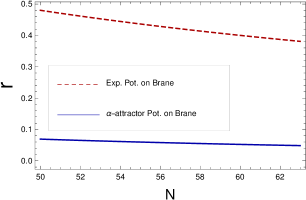
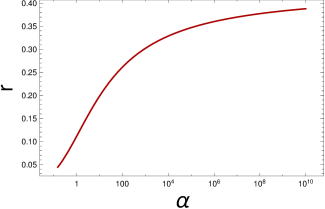
Now we will discuss some important results of our analysis one by one.

(i) N vs r :

From the Fig. 2, we see that we have a clear improvement for the value of $r$ those compared to the case standard exponential potential on the brane.

(ii) asymptotic value for $\alpha$ :

In the limit $\alpha\rightarrow\infty$, $\alpha$-attractor correction becomes irrelevantLinde:2016uec ; Dimopoulos:2017zvq and we get usual exponential potential. From the Fig. 2 it can be seen that $r$ approaches its asymptotic value as we increase the value of the parameter $\alpha$.

(iii)

It is worth noting that value of $r$ is insensitive to $\kappa$ in the original exponential potential, i.e $n$ for the potential (4) which we found to be same from the result we obtained in analytical approximation(35)

IV Approximated analytical results

An oversimplified approximation for the potential(4) can help us to get an approximate analytical result which we can use as a reference. To do so, we further simplify the potential in the limit $\varphi\rightarrow-\infty$ as

$$V\left(\varphi\right)\simeq M^{4}\left[1-2n\exp\left(\frac{2\sqrt{8\pi}}{\sqrt{6\alpha}\hskip 1.99168ptM_{Pl}}\varphi\right)\right].$$ (28)

The condition for end of inflation (11) gives

$$\frac{3\hskip 1.99168pt\alpha M^{4}M_{Pl}^{2}\hskip 1.99168pte^{-\frac{8\sqrt{\frac{\pi}{3}}}{\sqrt{\alpha}M_{Pl}}\varphi_{end}}}{64\pi n^{2}}\simeq\frac{5\lambda M_{Pl}^{2}}{24\pi}.$$ (29)

The Slow roll parameters(26,27) under this approximation become

$$\epsilon \simeq \frac{16\lambda\hskip 1.99168ptn^{2}\hskip 1.99168pte^{\frac{8\sqrt{\frac{\pi}{3}}\hskip 1.99168pt\varphi}{\sqrt{\alpha}\hskip 1.99168ptM_{Pl}}}}{3\hskip 1.99168pt\alpha\hskip 1.99168ptM^{4}\left(1-2\hskip 1.99168ptn\hskip 1.99168pte^{\frac{4\sqrt{\frac{\pi}{3}}\varphi}{\sqrt{\alpha}M_{Pl}}}\right)^{3}}\simeq\frac{16\lambda\hskip 1.99168ptn^{2}\hskip 1.99168pte^{\frac{8\sqrt{\frac{\pi}{3}}\hskip 1.99168pt\varphi}{\sqrt{\alpha}\hskip 1.99168ptM_{Pl}}}}{3\hskip 1.99168pt\alpha\hskip 1.99168ptM^{4}}.$$

$$\eta \simeq -\frac{8\hskip 1.99168pt\lambda\hskip 1.99168ptn\hskip 1.99168pte^{\frac{4\sqrt{\frac{\pi}{3}}}{\sqrt{\alpha}\hskip 1.99168ptM_{Pl}}\varphi}}{3\hskip 1.99168pt\alpha\hskip 1.99168ptM^{4}\left(1-2\hskip 1.99168ptn\hskip 1.99168pte^{\frac{4\sqrt{\frac{\pi}{3}}\hskip 1.99168pt\varphi}{\sqrt{\alpha}\hskip 1.99168ptM_{Pl}}}\right)^{2}}$$ (31)

$$\simeq -\frac{8\hskip 1.99168pt\lambda\hskip 1.99168ptn\hskip 1.99168pte^{\frac{4\sqrt{\frac{\pi}{3}}}{\sqrt{\alpha}\hskip 1.99168ptM_{Pl}}\hskip 1.99168pt\varphi}}{3\hskip 1.99168pt\alpha\hskip 1.99168ptM^{4}}.$$

The amplitude of the scalar perturbation(12)

$$A_{S}^{2} \simeq \left.\frac{M^{16}\hskip 1.99168pt\alpha}{25\hskip 1.99168pt\lambda^{3}\hskip 1.99168ptM_{Pl}^{4}\hskip 1.99168ptn^{2}}\hskip 1.99168pte^{-\frac{8\sqrt{\frac{\pi}{3}}\hskip 1.99168pt\varphi}{\sqrt{\alpha}\hskip 1.99168ptM_{Pl}}}\left(1-2\hskip 1.99168ptn\hskip 1.99168pte^{\frac{4\sqrt{\frac{\pi}{3}}\hskip 1.99168pt\varphi}{\sqrt{\alpha}\hskip 1.99168ptM_{Pl}}}\right)^{6}\right|_{k=aH}$$ (32)

$$\simeq \left.\frac{M^{16}\hskip 1.99168pt\alpha\hskip 1.99168pte^{-\frac{8\sqrt{\frac{\pi}{3}}\hskip 1.99168pt\varphi}{\sqrt{\alpha}\hskip 1.99168ptM_{Pl}}}}{25\hskip 1.99168pt\lambda^{3}\hskip 1.99168ptM_{Pl}^{4}\hskip 1.99168ptn^{2}}\right|_{k=aH}.$$

.

Figure 3: allowed region for $\alpha$ and $M^{4}/\lambda$ for $r\leq 0.06$

The number of $e$-foldings under this approximation is evaluated to be

$$N \simeq \int_{\varphi_{*}}^{\varphi_{end}}\frac{\sqrt{3\pi}\hskip 1.99168pt\sqrt{\alpha}\hskip 1.99168ptM^{4}}{2\hskip 1.99168ptn\hskip 1.99168pt\lambda\hskip 1.99168ptM_{Pl}}\hskip 1.99168pte^{-\frac{4\sqrt{\frac{\pi}{3}}\hskip 1.99168pt\varphi}{\sqrt{\alpha}\hskip 1.99168ptM_{Pl}}}\left(1-2\hskip 1.99168ptn\hskip 1.99168pte^{\frac{4\sqrt{\frac{\pi}{3}}\hskip 1.99168pt\varphi}{\sqrt{\alpha}\hskip 1.99168ptM_{Pl}}}\right)^{2}d\phi$$ (33)

$$\simeq \int_{\varphi_{*}}^{\varphi_{end}}\frac{\sqrt{3\pi}\hskip 1.99168pt\sqrt{\alpha}\hskip 1.99168ptM^{4}\hskip 1.99168pte^{-\frac{4\sqrt{\frac{\pi}{3}}\hskip 1.99168pt\varphi}{\sqrt{\alpha}M_{Pl}}}}{2\hskip 1.99168ptn\lambda\hskip 1.99168ptM_{Pl}}d\varphi\,\ .$$

Using condition of inflation end(29), we express $N$ in terms of field value at the horizon exit,

$$N\simeq\frac{3\hskip 1.99168pt\alpha\hskip 1.99168ptM^{4}\left(e^{-\frac{4\sqrt{\frac{\pi}{3}}\hskip 1.99168pt\varphi_{*}}{\sqrt{\alpha}\hskip 1.99168ptM_{Pl}}}-\frac{2\hskip 1.99168ptn\hskip 1.99168pt\sqrt{10}\hskip 1.99168pt\sqrt{\frac{\lambda}{\alpha}}}{3M^{2}}\right)}{8\hskip 1.99168pt\lambda\hskip 1.99168ptn}.$$ (34)

Using Eq. (34) and the fact $r=24\epsilon$, we find the tensor-to-scalar ratio from Eq. (LABEL:epsilonana),

$$r\simeq\frac{288\hskip 1.99168pt\alpha\hskip 1.99168pt\lambda\hskip 1.99168ptM^{4}}{\left(\sqrt{10}\hskip 1.99168pt\sqrt{\alpha\lambda}\hskip 1.99168ptM^{2}\hskip 1.99168pt+\hskip 1.99168pt4\hskip 1.99168ptN\hskip 1.99168pt\lambda\right)^{2}}\simeq\frac{288}{10\left(1+\frac{4N}{\sqrt{10\hskip 1.99168pt\alpha}\hskip 1.99168pt\sqrt{\frac{M^{4}}{\lambda}}}\right)^{2}}$$

(35)

The amplitude of scalar perturbation(32) is found to be

$$A_{S}^{2} \simeq \frac{4M^{8}\left(\sqrt{10}\hskip 1.99168ptM^{2}\sqrt{\alpha\lambda}\hskip 1.99168pt+\hskip 1.99168pt4\hskip 1.99168pt\lambda\hskip 1.99168ptN\right)^{2}}{225\alpha\hskip 1.99168pt\lambda^{3}\hskip 1.99168ptM_{Pl}^{4}}$$

$$\simeq \frac{8\left(\frac{M^{4}}{\lambda}\right)^{2}M^{4}}{45\hskip 1.99168ptM_{Pl}^{4}}\left(1+\frac{4N}{\sqrt{10\hskip 1.99168pt\alpha}\hskip 1.99168pt\sqrt{\frac{M^{4}}{\lambda}}}\right)^{2}.$$

It should be mentioned here that the relation given by the equations from (28)to (LABEL:AsqAna) represent only approximate expressions for the respective quantities. We see from (4) and (28) that this approximation breaks down for small values of $\varphi$ or $\alpha<1$ which is also confirmed by numerical results.

V Constraining model parameters from observations

In order to constrain the parameters of our model we stick to our numerical results. Firstly, we find that $r$ is independent of $M$, $\kappa$ and depends only on the ratio $\frac{M^{4}}{\lambda}$ and $\alpha$.

Figure 4: $68\%$ (red) and $95\%$ (black) contour regions($n_{S}$-$r$ plane) taken from Planck 2018 results(TT, TE, EE+lowE+lensing+BK14+BAO)Akrami:2018odb , we overlay our model’s result on it. We obtain our results by varying $\alpha$ from 0.16 to 10. For both the figures black dot and green dot correspond $\alpha=5$ and 0.5 respectively. The solid blue line is for $N=60$. For the top Fig., $\frac{M^{4}}{\lambda}=40$ and for the bottom Fig., $\frac{M^{4}}{\lambda}=20$.

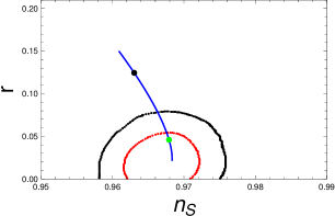
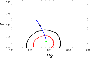
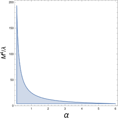
The observational constraint on the parameter, $r\lesssim 0.06$ planck ; Ade:2018gkx ; Akrami:2018odb , allows us to constrain the parameter $\alpha$ and the ratio $M^{4}/\lambda$. Theoretically, the high energy limit corresponds $\frac{M^{4}}{\lambda}\gg 1$, but this ratio is highly dependent on the other parameter $\alpha$ under observational bound. A higher value of the parameter $\alpha$ limits the parameter $M^{4}/\lambda$ to a lower value. In other words, a decent limit of the assumption that during inflation $M^{4}/\lambda\gg 1$ pushes $\alpha$ to a lower value. The bound $\alpha\leq 39.6$, in the reference Dimopoulos:2017zvq is reduced to $\alpha\lesssim 3.6$ for a value of $M^{4}/\lambda\gtrsim 7$. In Fig. 3, we show the allowed values of $\alpha$ against $M^{4}/\lambda$. In Fig. 4, we compare our results for different parameters’ value with Planck 2018 resultsAkrami:2018odb .

The non-canonical scalar degrees of freedom, $\phi$ remains sub-Planckian as long as $\alpha\lesssim\frac{1}{6}$(2). We can obtain this bound in a more compelling way in our model if we consider $\frac{M^{4}}{\lambda}\gtrsim 150$ along with the observational bound $r\lesssim 0.06$. In other words, the value of $\frac{M^{4}}{\lambda}$, nearly bigger than $150$ will always keep the non-canonical scalar degree of freedom within a sub-Planckian value.

$\alpha$	$M$(GeV)
$0.167$	$1.69\times 10^{15}$
$1$	$4.15\times 10^{15}$
$10$	$1.31\times 10^{16}$

Table 1: Values of $M$ for different $\alpha$, $\lambda$ is taken as allowed by $r$

The COBE normalization corresponds to the amplitude of the scalar perturbations (see Eq. (12)) $A_{S}\simeq 2\times 10^{-5}$cobe1 , which along with the bound on $\alpha$ determines the energy scale of inflation. We found that (Table-1) it is near the grand unification scale, almost same as the one in standard inflationary cosmology. Consequently, after inflation ends, the field will have large overshoot below the background freezing itself for a long time; only at late times it will evolve mimicking cosmological constant like behavior.

VI Late time behavior

Let us briefly comment on the post inflationary features of the model. First, the brane corrections to Freidmann equation are insignificant in the post inflationary era. Secondly, it is interesting that irrespective of the nature of original exponential potential, the $\alpha$ attractor effective potential, see Fig. 1 has a generic form, namely, it has plateau followed by a sharp steep behavior like a water fall settling fast to a constant value thereafter. In this case, the trackersami:track ; Sami:2009jx ; Sami:2009dk ; Steinhardt:1999nw behavior is inherently absent which makes the dynamics of scalar field sensitive to its initial conditions. The thawing behaviour in the model under consideration can be understood analytically. Actually, the important features of dynamics are encoded in a quantity

Figure 5: The figure shows the behavior of $\Gamma$ with $\varphi$, for potential (3) with a residual vacuum energy density $V_{0}e^{-\kappa\sqrt{6\alpha}}$ subtracted from the standard exponential potential in (1) as taken in the Refs. Dimopoulos:2017zvq ; Dimopoulos:2017tud

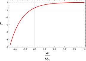
, the dashed line represents a constant value 1.

dubbed $\Gamma$ which for the potential (3) is given by,

$$\Gamma(\varphi) \equiv \frac{V(\varphi)^{\prime\prime}V(\varphi)}{V(\varphi)^{\prime 2}}$$ (37)

$$= \frac{e^{-n}}{n}\left\{e^{n}-e^{n\tanh\left(\frac{2\sqrt{2\pi/3}}{M_{Pl}\sqrt{\alpha}}\varphi\right)}\right\}$$

$$\times\left\{n+\sinh\left(\frac{4\sqrt{2\pi/3}}{M_{Pl}\sqrt{\alpha}}\varphi\right)\right\}$$

Eq. (37) tells us that $\Gamma$ increases fast with $\phi$ and crosses zero and approaches unity thereafter mimicking the exponential behaviour, see Fig.5. On the other hand, to realize tracker behavior, it is necessary that $\Gamma$ being greater than unity stays close to one for long time such that the field approximately mimics the background. In the present case the slope of the potential,starting from a large value, gradually diminishes pushing the system to slow roll regime at late times. Thus owing to the behavior of $\Gamma$ in Fig. 5, the field energy density would witness the large overshoot with respect to the backgrouund in a short span of time freezing the field on its potential due to large Hubble damping. Field evolution would commence only at late stages when background energy density becomes comparable to field energy density allowing the slow roll of field giving rise to late time acceleration; slow roll is characterized by shallow exponential like behaviour. Hence, the present scenario gives rise to thawing behaviour as noticed in Ref.Dimopoulos:2017zvq ; Akrami:2017cir .

VII Conclusion

In this paper, we have considered an inflationary scenario in $\alpha$-attractor framework for an exponential potential on RS brane. We have carried out full numerical analysis and presented approximated analytical results. We have found that our results pass the observational constraint for suitable parameter values. The observational bound on the parameter tensor to scalar ratio, $r\leq 0.06$Ade:2018gkx ; Akrami:2018odb is easily satisfied by our model for a range of parameters$-$ $\alpha\lesssim 3.6$ with $M^{4}/\lambda\gtrsim 7$. We found that a lower values of the parameter $\alpha$ gives rise to a large range of the parameter $M^{4}/\lambda$, falling within the window allowed by observations(Fig. 3). The lower bound on $\alpha$, related to the inflation scale,$\alpha\gtrsim 10^{-7}$Dimopoulos:2017zvq , is not considered here to compare with observational consistency. The significance of the brane correction underlies with the assumption that $V/\lambda\gg 1$ or equivalently $M^{4}/\lambda\gg 1$ during inflation which automatically pushes $\alpha$ toward a lower values in order to meet observational constraints. We numerically found that for consistency with observation, $M^{4}/\lambda\gtrsim 150$ corresponds to $\alpha<1/6$ which keeps the non-canonical scalar field to be sub-Planckian. It is worth mentioning that we do not attempt to constrain here the parameters $V_{0}$ and $\kappa$ directly as done in Dimopoulos:2017zvq ; Dimopoulos:2017tud , however, by constraining $\frac{M^{4}}{\lambda}$ and $\alpha$ puts some indirect constraints on these parameters. In Ref Dimopoulos:2017tud a rather tight bound is given on the parameter $\alpha$ based on the dark energy observations and the super-Planckian issue, $1.5\leq\alpha\leq 4.2$. Our analysis is compatible with this value as we can see from Fig. 3. We also find that our inflation is scale is near the grand unification scale, same as the case for standard inflationary models. As for the post inflationary evolution, we have argued based upon our analytical expressions that the scenario under consideration should give rise to thawing behaviour, see Fig.5 and discussion in section V noticed numerically in Refs.Dimopoulos:2017zvq ; Dimopoulos:2017tud . The Present work, with high numerical precision, can be extended to obtain more accurate bounds on the parameters. The other aspects associated with inflation like reheating can also be investigated for the model under consideration. The investigation of alternative reheating suitable to the the present framework is left for future work.

References

- (1) A.D. Linde, Phys. Lett. B,129B,177 (1983); A. D. Linde, [arXiv:0705.0164 [hep-th]]; A. R. Liddle, astro-ph/9901124.
- (2) K. Akama, Lect. Notes Phys. 176, 267 (1982) [hep-th/0001113]; N. Arkani-Hamed, S. Dimopoulos and G. R. Dvali, Phys. Lett. B 429, 263 (1998) [hep-ph/9803315]; L. Randall and R. Sundrum, Phys. Rev. Lett. 83, 3370 (1999) [hep-ph/9905221]; A. R. Liddle and A. N. Taylor, Phys. Rev. D 65, 041301 (2002) [astro-ph/0109412].
- (3) L. Randall and R. Sundrum, Phys. Rev. Lett. 83, 4690 (1999) [hep-th/9906064].
- (4) T. Shiromizu, K. i. Maeda and M. Sasaki, Phys. Rev. D 62, 024012 (2000) [gr-qc/9910076].
- (5) P. Binetruy, C. Deffayet, U. Ellwanger and D. Langlois, Phys. Lett. B 477, 285 (2000) [hep-th/9910219]; P. Binetruy, C. Deffayet and D. Langlois, Nucl. Phys. B 565, 269 (2000) [hep-th/9905012].
- (6) R. Maartens, D. Wands, B. A. Bassett and I. Heard, Phys. Rev. D 62, 041301 (2000) [hep-ph/9912464] .
- (7) J. M. Cline, C. Grojean and G. Servant, Phys. Rev. Lett. 83, 4245 (1999) [hep-ph/9906523];C. Csaki, M. Graesser, C. F. Kolda and J. Terning, Phys. Lett. B 462, 34 (1999) [hep-ph/9906513]; D. Ida, JHEP 0009, 014 (2000) [gr-qc/9912002].
- (8) Y. g. Gong, gr-qc/0005075.
- (9) P. S. Apostolopoulos, N. Brouzakis, E. N. Saridakis and N. Tetradis, Phys. Rev. D 72, 044013 (2005) [hep-th/0502115].
- (10) V. Sahni, M. Sami and T. Souradeep, Phys. Rev. D 65, 023518 (2002) [gr-qc/0105121].
- (11) M. Sami and V. Sahni, Phys. Rev. D 70, 083513 (2004) [hep-th/0402086].
- (12) E. J. Copeland, A. R. Liddle and J. E. Lidsey, Phys. Rev. D 64, 023509 (2001) [astro-ph/0006421].
- (13) F. Lucchin and S. Matarrese Phys. Rev. D 32, 1316 (1985).
- (14) S. Tsujikawa and A. R. Liddle, JCAP 0403, 001 (2004) [astro-ph/0312162].
- (15) P. A. R. Ade et al. [Planck Collaboration], Astron. Astrophys. 594, A13 (2016) [arXiv:1502.01589 [astro-ph.CO]].
- (16) P. A. R. Ade et al. [BICEP2 and Keck Array Collaborations], Phys. Rev. Lett. 116, 031302(2016)[arXiv:1510.09217 [astro-ph.CO]].
- (17) P. A. R. Ade et al. [BICEP2 and Keck Array Collaborations], Phys. Rev. Lett. 121, 221301 (2018) [arXiv:1810.05216 [astro-ph.CO]].
- (18) Y. Akrami et al. [Planck Collaboration], arXiv:1807.06211 [astro-ph.CO].
- (19) A. Linde, JCAP 1702, no. 02, 028 (2017) [arXiv:1612.04505 [hep-th]].
- (20) K. Dimopoulos and C. Owen, JCAP 1706, no. 06, 027 (2017) [arXiv:1703.00305 [gr-qc]].
- (21) K. Dimopoulos, L. Donaldson Wood and C. Owen, Phys. Rev. D 97, no. 6, 063525 (2018) [arXiv:1712.01760 [astro-ph.CO]].
- (22) Y. Akrami, R. Kallosh, A. Linde and V. Vardanyan, JCAP 1806, no. 06, 041 (2018) doi:10.1088/1475-7516/2018/06/041 [arXiv:1712.09693 [hep-th]].
- (23) M. Shahalam, M. Sami and A. Wang, arXiv:1806.05815 [astro-ph.CO].
- (24) M. Shahalam, R. Myrzakulov, S. Myrzakul and A. Wang, Int. J. Mod. Phys. D 27, no. 05, 1850058 (2018) [arXiv:1611.06315 [astro-ph.CO]].
- (25) C. García-García, E. V. Linder, P. Ruíz-Lapuente and Miguel Zumalacárregui, arXiv:1803.00661 [astro-ph.CO]. Phys. Rev. D 97, no. 6, 063525 (2018) [arXiv:1712.01760 [astro-ph.CO]].
- (26) P. J. E. Peebles and A. Vilenkin, Phys. Rev. D 59, 063505 (1999) [astro-ph/9810509].
- (27) E. J. Copeland, M. Sami and S. Tsujikawa, Int. J. Mod. Phys. D 15, 1753 (2006) [hep-th/0603057].
- (28) M. Wali Hossain, R. Myrzakulov, M. Sami and E. N. Saridakis, Int. J. Mod. Phys. D 24, no. 05, 1530014 (2015) [arXiv:1410.6100 [gr-qc]].
- (29) S. S. Mishra, V. Sahni and Y. Shtanov, JCAP 1706, no. 06, 045 (2017) [arXiv:1703.03295 [gr-qc]].
- (30) M. Sami and N. Dadhich, TSPU Bulletin 44N7, 25 (2004) [hep-th/0405016].
- (31) J. Rubio and C. Wetterich, Phys. Rev. D 96, no. 6, 063509 (2017) [arXiv:1705.00552 [gr-qc]].
- (32) Quintessence: The fifth force - Wetterich, C. Physik J. 3N12 (2004) 43-48
- (33) K. Dimopoulos, Phys. Rev. D 68, 123506 (2003) [astro-ph/0212264].
- (34) R. K. Kaul, arXiv:0803.0381 [hep-ph].
- (35) D. Langlois, R. Maartens and D. Wands, Phys. Lett. B 489, 259 (2000) [hep-th/0006007].
- (36) B. R. Dinda, S. Kumar and A. A. Sen, Phys. Rev. D 90, no. 8, 083515 (2014) [arXiv:1404.3683 [astro-ph.CO]].
- (37) E. F. Bunn, A. R. Liddle and M. J. White, Phys. Rev. D 54, no. 10, R5917 (1996) [astro-ph/9607038]; E. F. Bunn and M. J. White, Astrophys. J. 480, 6 (1997) [astro-ph/9607060].
- (38) M. Sami, Curr. Sci. 97, 887 (2009) [arXiv:0904.3445 [hep-th]]. JCAP 1706, no. 06, 045 (2017) [arXiv:1703.03295 [gr-qc]].
- (39) Models of Dark Energy M. Sami, Center forTheoretical Physics, Jamia Millia Islamia, New Delhi, India, https://www.ctp-jamia.res.in/people/models_of_dark_energy.pdf.
- (40) M. Sami, arXiv:0901.0756 [hep-th].
- (41) P. J. Steinhardt, L. M. Wang and I. Zlatev, Phys. Rev. D 59, 123504 (1999) [astro-ph/9812313].