Energy Constraints and Phenomenon of Cosmic Evolution in $f(T,B)$ Framework

Abstract

We investigate the cosmological evolution in a new modified teleparallel theory, called $f(T,B)$ gravity, which is formulated by connecting both $f(T)$ and $f(R)$ theories with a boundary term $B$. Here, $T$ is the torsion scalar in teleparallel gravity and $R$ is the scalar curvature. For this purpose, we assume flat Friedmann-Robertson-Walker (FRW) geometry filled with perfect fluid matter contents. We study two cases in this gravity: One is for a general function of $f(T,B)$, and the other is for a particular form of it given by the term of $-T+F(B)$. We also formulate the general energy constraints for these cases. Furthermore, we explore the validity of the bounds on the energy conditions by specifying different forms of$f(T,B)$ and $F(B)$ function obtained by the reconstruction scheme for de Sitter, power-law, the $\Lambda$CDM and Phantom cosmological models. Moreover, the possible constraints on the free model parameters are examined with the help of region graphs. In addition, we explore the evolution of the effective equation of state (EoS) $\omega_{eff}$ for the universe and compare theoretical results with the observational data. It is found that the effective EoS represents the phantom phase or the quintessence one in the accelerating universe in all of the cases consistent with the observational data.

Keywords: Modified gravity; Energy Conditions; Cosmic Evolution.

I Introduction

In the recent past, the development of a modified gravitational framework that can successfully demonstrates the total cosmic matter contents along with the complete history of cosmic evolution (from big bang phenomenon till its final fate) is regarded as one of big challenges. Although general theory of relativity (GR) is regarded as a very successful theory that is consistent with the observational results however it has some limitations on dark matter and DE. So, the work on the modification of GR started just after it’s formulation. In this respect, Weyl made an effort for combining the gravitation and electromagnetism soon after the final presentation of GR 1 . His effort was not as much successful but it initiated the concept of gauge transformation and gauge invariance and thus provided a basis for gauge theory 2 ; 3 . Ten years later, Einstein 4 made an effort by constructing the structure of teleparallelism. In his effort, he used the concept of tetrad, an orthogonal field based on the four-dimensional space-time tangent space. As the tetrad has sixteen components, therefore Einstein called this structure as a unification of electromagnetism and gravity by relating six additional degrees of freedom to electromagnetic field. Later on, it was also not proved as problem free but the main idea of this theory is considered important till date.

In this respect, Kaluza 5 and Klein 6 also proposed an unified platform for gravity and electromagnetism, called Kaluza-Klein theory. Further Cartan presented a successful modification of GR, namely Einstein-Cartan theory, in which spacetime involves both curvature and torsion 7 ; 8 . In this theory, energy and momentum were the source of curvature, while the spin was the source of torsion. In 1960, Moller 9 ; 10 made an effort based on Einstein’s idea to find a tensorial complex which is invariant under coordinate transformation but not under local Lorentz transformation. On the basis of Moller’s work, Pellegrini and Plebanski 11 found a formulation of Lagrangian for teleparallel gravity. In 1976, Cho 12 found teleparallel Lagrangian with the coefficient of anholonomy by replacing torsion and it was invariant under local Lorentz transformation. In 1979, Hayashi and Shirafuji 13 made an effort to unify the concept of teleparallelism with his earlier proposed gauge theory 14 ; 15 ; 16 .

Teleparallel gravity (TG) is a modified theory that is equivalent to GR based on a different concept, like GR determines trajectories by geodesics but TG consider torsion as a responsible candidate for gravitation. Weitznb$\ddot{o}$ck suggested that it is possible to choose such a connection for which the curvature vanishes and this is regarded as a main idea behind teleparallel theory. Interestingly, the field equations obtained through this formulation are equivalent to that of GR 17 ; 18 . The interest in TG is raising day by day over past few decades and many other extensions of this theory has been proposed in literature 19 . One of its interesting modification is $f(T,T_{G})$ gravity involving torsion invariant T and contribution from a term $T_{G}$, the teleparallel equivalent of the Gauss-Bonnet term 20 . Another modification involves general $f(T)$ function and its non-minimal coupling with matter 21 . Much work has been done on these teleparallel frameworks and researchers obtained viable results for various cosmological issues (for reviews on modified gravity and dark energy problem to account for the late-time cosmic acceleration, see, e.g., Nojiri:2006ri ; Nojiri:2010wj ; Book-Capozziello-Faraoni ; Capozziello:2011et ; Bamba:2012cp ; Joyce:2014kja ; Koyama:2015vza ; Bamba:2015uma ; Cai:2015emx ; Nojiri:2017ncd ).

$R=-T+B$ is the one of the basic equation of GR and its teleparallel equivalent, where $R$ is the Ricci scalar, $T$ is the torsion scalar and $B$ is a total derivative term which only depends on torsion, named as boundary term. Thus Einstein-Hilbert action can be represented by either using Ricci scalar or the torsion scalar as it gives identical equations of motion. It is worthwhile to mention here that variation of $f(R)$ Lagrangian (modification of GR) results in fourth order field equations 22 ; 23 while $f(T)$ Lagrangian leads to second order field equations 24 . As the terms $T$ and $B$ are not invariant and hence under local Lorentz transformation, this theory is no longer invariant 25 ; 26 , but this issue can be resolved by taking the particular combination $-T+B$ 27 . So the $f(R)$ and $f(T)$ theories are not equivalent but a relationship can be developed by using theories based on $f(T,B)$ functions. In 28 , Bahamonde et al. reconstructed some well known models in the background of $f(T,B)$ gravity, discussing the thermodynamic properties and stability of such models.

The investigation of possible bounds on free parameters arising from different DE models by making them consistent with the energy conditions has always been a center of interest for the researchers. Such constraints have already been explored in various gravitational frameworks like $f(R)$ gravity, $f(T)$ theory, $f(G)$ theory, $f(R)$ gravity involving non-minimal interaction with matter, $f(R,\mathcal{L}_{m})$ gravity and Brans-Dicke theory 29 . In this context, Sharif and Saira 30 considered FRW geometry with perfect fluid matter contents in the most general scalar-tensor gravity involving second-order derivatives of scalar field in field equations and discussed the possible validity of energy conditions. Sharif and Zubair 31 have investigated the consistency of these bounds in $f(R,T)$ gravity that involves Ricci scalar and energy-momentum tensor trace. By using power law cosmology, they also developed the stability criteria for this configuration. Further, in another study, they examined some models of $f(R,T,R_{\mu\nu}T^{\mu\nu})$ gravity using energy inequalities 32 . Zubair and Waheed studied the validity of energy bounds for power law FRW cosmology in a modified theory involving non-minimal coupling of torsion scalar and perfect fluid matter 21 . In another paper 33 , the same authors explored the compatibility of energy constraints in $F(T,T_{G})$ gravity using two different proposed models of $F(T,T_{G})$ for FRW geometry with perfect fluid matter and obtained interesting results.

Being motivated from the literature, in the present manuscript, we investigate the possible constraints on free parameters using energy condition approach in $f(T,B)$ gravity. In the next section, we present a brief formulation of this theory and its resulting field equations for perfect fluid FRW geometry. In section III, we formulate the energy constraints for a general $f(T,B)$ function as well as its specific form $-T+F(B)$. Section IV is devoted to study these energy bounds for four different $f(T,B)$ models obtained by reconstruction scheme namely: de sitter universe, power law cosmology, $\Lambda$CDM model and phantom cosmology. Here we discuss the validity of energy conditions and evolution of effective equation of state (EoS) parameter using graphs. In the next section, we discuss these energy bounds for particular forms of $-T+F(B)$ constructed by reconstruction scheme using all four cases. Last section concludes the whole discussion and highlights the major results.

II Basic Formulation of $f(T,B)$ theory of gravity and FRW geometry

In this section, we discuss the basic notions of $f(T,B)$ gravity and construct the corresponding field equations for flat FRW geometry with perfect fluid matter source. For this purpose, we consider the action of a modified version of teleparallel theory proposed in a recent study 27 given as follows

$$S_{f(T,B)}=\frac{1}{\kappa^{2}}\int dx^{4}\,e\,f(T,B)+S_{\rm m}\,,$$ (1)

where $f(T,B)$ is a general function of torsion scalar $T$ and boundary term $B$. Here $e$ represents the determinant of tetrad and $S_{m}$ denotes the action of ordinary matter. Actually, Ricci scalar of Levi-civita in terms of torsion can be written in the form:

$$R(e)=-T+\frac{2}{e}\partial_{\mu}(eT^{\mu}),$$ (2)

where the term in addition involving torsion vector $T^{\mu}$ is considered as the boundary term given by $B=\frac{2}{e}\partial_{\mu}(eT^{\mu})$. It has been proved that by choosing $f=f(T)$ and $f=f(-T+B)=f(R)$, it is possible to recover both $f(T)$ and $f(R)$ theories, respectively. The variation of the above action with respect to tetrad results in the following set of field equations

$$2e\delta^{\lambda}_{\nu}\Box f_{B}-2e\nabla^{\lambda}\nabla_{\nu}f_{B}+eBf_{B}\delta^{\lambda}_{\nu}+4e\big{[}(\partial_{\mu}f_{B})+(\partial_{\mu}f_{T})\big{]}S^{\mu\lambda}_{\nu}+4e^{a}_{\nu}\partial_{\mu}(eS^{\mu\lambda}_{a})f_{T}-4ef_{T}T^{\sigma}_{\mu\nu}S_{\sigma}^{\lambda\mu}-ef\delta_{\nu}^{\lambda}=16\pi e\tau^{\lambda}_{\nu},$$ (3)

where $\tau_{\nu}^{\lambda}=e_{\nu}^{a}\tau_{a}^{\lambda}$ is standard energy-momentum tensor and $\Box=\nabla^{\mu}\nabla_{\mu}$.

The line element for flat FRW geometry is given by

$$ds^{2}=-dt^{2}+a(t)^{2}(dx^{2}+dy^{2}+dz^{2}),$$ (4)

where $a(t)$ is the expansion radius of universe. In these coordinates, the tetrad field can be expressed as follows

$$e_{\mu}^{a}=\text{{diag}}\left(1,a(t),a(t),a(t)\right)\,.$$ (5)

We assume the source of ordinary matter as perfect fluid given by

$$T_{\mu\nu}=(\rho_{m}+p_{m})u_{\mu}u_{\nu}-p_{m}g_{\mu\nu},$$ (6)

where $\rho_{m}$ and $p_{m}$ are ordinary matter density and pressure, respectively.

Using (4) along with (6), the corresponding field equations (3) takes the following form

$$-3H^{2}(3f_{B}+2f_{T})+3H\dot{f}_{B}-3\dot{H}f_{B}+\frac{1}{2}f(T,B)=\kappa^{2}\rho_{m},$$ (7)

$$-3H^{2}(3f_{B}+2f_{T})-\dot{H}(3f_{B}+2f_{T})-2H\dot{f}_{T}+\ddot{f}_{B}+\frac{1}{2}f(T,B)=-\kappa^{2}p_{m}.$$ (8)

Here $H=\frac{\dot{a}}{a}$ is the Hubble parameter and dot represents derivative with respect to $t$. In terms of effective energy and pressure terms, the above set of equations can be rewritten as

$$3H^{2}=\kappa^{2}_{eff}(\rho_{eff}),$$ (9)

$$2\dot{H}=-\kappa^{2}_{eff}(\rho_{eff}+p_{eff}),$$ (10)

where

$$\rho_{eff}=\rho_{m}+\frac{1}{\kappa^{2}}\bigg{[}-3H\dot{f}_{B}+(3\dot{H}+9H^{2})f_{B}-\frac{1}{2}f(T,B)\bigg{]},$$ (11)

$$p_{eff}=p_{m}+\frac{1}{\kappa^{2}}\bigg{[}\frac{1}{2}f(T,B)+\dot{H}(2f_{T}-3f_{B})-2H\dot{f}_{T}-9H^{2}f_{B}+\ddot{f}_{B}\bigg{]}.$$ (12)

III Energy Conditions

In this section, firstly, we present a general discussion on energy condition bounds in GR and then formulate specifically these constraints for the present case. The origin of these conditions emerges from the Raychaudhuri equation along with the condition that the gravity is attractive. For this, consider the tangent vector field $u^{\mu}$ that is congruent to timelike geodesics in a spacetime manifold endowed with a metric $g_{\mu\nu}$. Then Raychaudhuri’s equation is given by

$$\frac{d\theta}{d\tau}=-\frac{1}{3}\theta^{2}-\sigma_{\mu\nu}\sigma^{\mu\nu}-\omega_{\mu\nu}\omega_{\mu\nu}-R_{\mu\nu}u^{\mu}u^{\nu},$$ (13)

where terms $R_{\mu\nu},~{}\theta$ and $\sigma^{\mu\nu}$ denote the Ricci tensor, expansion, and shear scalars, respectively. Also, $\omega_{\mu\nu}$ is the rotation associated to the congruence defined by the vector field $u^{\mu}$. The above equation deals with the geometry and has no reference to gravitational field equations. Since the GR field equations relate Ricci tensor $R_{\mu\nu}$ to the energy-momentum tensor $T_{\mu\nu}$, therefore the combination of Einstein’s and Raychaudhuri’s equations can be used to restrict the energy-momentum tensor on physical grounds. As the shear is spatial tensor and $\sigma^{2}\equiv\sigma_{\mu\nu}\sigma^{\mu\nu}\geq 0$, so from Raychaudhuri’s equation, the condition for attractive gravity $\frac{d\theta}{d\tau}<0$ reduces to $R_{\mu\nu}u^{\mu}u^{\nu}\geq 0$ for any hypersurface orthogonal congruences ($\omega\equiv 0$). Consequently, by using Einstein’s equation, it can be written as

$$R_{\mu\nu}u^{\mu}u^{\nu}=\left(T_{\mu\nu}-\frac{T}{2}g_{\mu\nu}\right)u^{\mu}u^{\nu}\geq 0.$$ (14)

Here we consider $8\pi G=c=1$. Further, symbols $T_{\mu\nu}$ and $T$ represent the energy-momentum tensor and its trace, respectively.

Equation (14) gives the strong energy condition (SEC) in a coordinate-invariant way in terms of $T_{\mu\nu}$. So SEC in the context of GR shows that the gravity is attractive. For a perfect fluid matter source (6), Eq.(14) takes the form as $\rho_{m}+3p_{m}\geq 0$. Other energy constraints namely null energy condition (NEC), weak energy condition (WEC) and dominant energy conditions (DEC) can be written as

$$NEC:\rho_{m}+p_{m}\geq,~{}WEC:\rho_{m}\geq 0,~{}\rho_{m}+p_{m}\geq 0,~{}DEC:\rho_{m}\geq 0,~{}\rho_{m}\pm p_{m}\geq 0.$$

The derivation of energy conditions for $f(T,B)$ gravity can be done in a similar pattern. In the present work, we consider that the total matter contents acts as a perfect fluid. So these conditions can be obtained by just replacing $\rho_{m}$ with $\rho_{eff}$ and $p_{m}$ with $p_{eff}$ as follows

$$NEC : ~{}\rho_{eff}+p_{eff}=\rho_{m}+p_{m}+\frac{1}{\kappa^{2}}\bigg{[}-3H\dot{f}_{B}+3\dot{H}f_{B}+\dot{H}(3f_{B}+2f_{T})-2H\dot{f}_{T}+\ddot{f}_{B}\bigg{]}\geq 0,$$ (15)

$$WEC : ~{}\rho_{eff}=\rho_{m}+\frac{1}{\kappa^{2}}\bigg{[}-3H\dot{f}_{B}+3\dot{H}f_{B}-\frac{1}{2}f(T,B)\bigg{]}\geq 0,~{}\rho_{eff}+p_{eff}\geq 0,$$ (16)

$$SEC : ~{}\rho_{eff}+3p_{eff}=\rho_{m}+3p_{m}+\frac{1}{\kappa^{2}}\bigg{[}-3H\dot{f}_{B}+12\dot{H}f_{B}+f(T,B)+6\dot{H}f_{T}-6H\dot{f}_{T}+3\ddot{f}_{B}\bigg{]}\geq 0,$$ (17)

$$\rho_{eff}+p_{eff}\geq 0,$$

$$DEC : ~{}\rho_{eff}-p_{eff}=\rho_{m}-p_{m}+\frac{1}{\kappa^{2}}\bigg{[}-3H\dot{f}_{B}-2\dot{H}f_{T}+2H\dot{f}_{T}-\ddot{f}_{B}-f(T,B)\bigg{]}\geq 0,$$ (18)

$$\rho_{eff}\geq 0,~{}\rho_{eff}+p_{eff}\geq 0.$$

Inequalities (15)-(18) represents the null, weak, strong and dominant energy conditions in the context of $f(T,B)$ gravity for $FRW$ spacetime.

For flat FRW spacetime, the torsion scalar and the boundary term takes the form:

$$T=6H^{2},\quad B=6(\dot{H}+3H^{2}).$$

Also, for FRW line element, deceleration, jerk and snap cosmological parameters are given by

$$q=-\frac{1}{H^{2}}\frac{\ddot{a}}{a},\quad j=\frac{1}{H^{3}}\frac{\dddot{a}}{a},\quad s=\frac{1}{H^{4}}\frac{\ddddot{a}}{a}$$

The expressions of $T,~{}B$ and $H$ along with their derivatives in terms of these cosmological parameters can be written as

$$T = 6H^{2},\quad\dot{T}=-12H^{3}(1+q),\quad B=6H^{2}(2-q),\quad\dot{B}=6H^{3}(j-3q-4),$$

$$H = \frac{\dot{a}}{a},\quad\dot{H}=-H^{2}(1+q),\quad\ddot{H}=(j+3q+2)H^{3},\quad\dddot{H}=H^{4}(s-4j-12q-3q^{2}-6).$$

Using the above definitions, the energy conditions (15)-(18) will take the form as follows

$$NEC : \kappa^{2}(\rho_{m}+p_{m})-2H^{2}(1+q)(3f_{B}+f_{T})-18H^{4}(j-3q-4)f_{BB}+36H^{4}(1+q)$$ (19)

$$- 12H^{4}(j-3q-4)f_{BT}-24H^{4}(1+q)f_{TT}+36H^{6}(j-3q-4)^{2}f_{BBB}$$

$$- 144H^{6}(1+q)(j-3q-4)f_{BBT}+144H^{6}(1+q)^{2}f_{BTT}\geq 0,$$

$$WEC : \kappa^{2}\rho_{m}-18H^{4}(j-3q-4)f_{BB}+36H^{4}(1+q)f_{BT}-3H^{2}(1+q)f_{B}-\frac{1}{2}f(T,B)\geq 0,$$ (20)

$$\rho_{eff}+p_{eff}\geq 0,$$

$$SEC : \kappa^{2}(\rho_{m}+3p_{m})-18H^{4}(j-3q-4)f_{BB}+36H^{4}(1+q)f_{BT}-12H^{2}(1+q)f_{B}-6H^{2}(1+q)f_{T}$$ (21)

$$- 36H^{4}(j-3q-4)f_{BT}+72H^{4}(1+q)f_{TT}+108H^{6}(j-3q-4)^{2}f_{BBB}-72H^{6}(1+q)(j-3q-4)f_{BBT}$$

$$+ 432H^{6}(1+q)f_{BTT}+f(T,B)\geq 0,\quad\rho_{eff}+p_{eff}\geq 0,$$

$$DEC : \kappa^{2}(\rho_{m}-p_{m})-18H^{4}(j-3q-4)f_{BB}+12H^{4}(1+q)f_{BT}+2H^{2}(1+q)f_{T}-24H^{4}(1+q)f_{TT}$$ (22)

$$-36H^{6}(j-3q-4)f_{BBB}-144H^{6}(1+q)(j-3q-4)f_{BBT}+144H^{6}(1+q)^{2}f_{BTT}-f(T,B)\geq 0,$$

$$\rho_{eff}+p_{eff}\geq 0,\quad\rho_{eff}\geq 0.$$

IV Evolution of Energy condition Bounds using Reconstructed Models of $f(T,B)$

In this section, we explore the evolution of energy condition bounds (19)-(22) using some interesting $f(T,B)$ models obtained by reconstruction scheme. For this purpose, we consider four well-known cosmological models namely de Sitter (dS), power law, $\Lambda$CDM and phantom models of cosmos.

IV.1 de Sitter universe model

The dS solutions are considered as one of the most fascinating models in cosmology for explaining the current accelerated cosmic epoch. The dS model is described by the exponential scale factor defined as $a(t)=a_{0}e^{H_{0}t}$, where $a_{0}$ and $H_{0}$ are the present values of scale factor and Hubble parameter, respectively. Further, the torsion scalar and the boundary term takes the form:

$$T=6H_{0}^{2},~{}B=18H_{0}^{2}.$$

Also, we consider the perfect fluid matter source satisfies constant EoS parameter given by $\omega_{m}=\frac{p_{m}}{\rho_{m}}$. Thus,

$$\rho=\rho_{0}e^{-3(1+\omega_{m})H_{0}t},\quad\rho_{m}=\rho_{0}a(t)^{-3(\omega_{m}+1)},\quad p_{m}=\omega_{m}\rho_{m}.$$

Consequently, the reconstruction technique leads to the following form of $f(T,B)$ model given by

$$f(T,B)=2(\kappa^{2}\rho_{0}+2K)+f_{0}e^{\frac{B}{18H_{0}^{2}}}+\widetilde{f}_{0}e^{\frac{T}{12H_{0}^{2}}}.$$ (23)

Here $f_{0}$ and $\widetilde{f}_{0}$ are integration constants, while $K$ is the constant of separation. Introducing Eq.(23) in the set of energy conditions (19) and (22), we get

$$NEC : e(-2+j^{2}-3q+9q^{2}-j(17+6q))f_{0}+54(1+q)(108H_{0}^{4}-\sqrt{e}\widetilde{f}_{0})\geq 0,$$

$$WEC : e(8+j)f_{0}+9\left(4K+\sqrt{e}\tilde{f}_{0}\right)\geq 0,\quad NEC\geq 0.$$

Here, each of these inequalities depend on the values of $j,~{}q,~{}H_{0},~{}f_{0},~{}K$ and $\tilde{f_{0}}$. For graphical illustration, we consider the recent values of cosmic parameters $H_{0}$, $q$ and $j$. proposed by Capozziello et al. 34 . These values are $H_{0}=0.718,~{}q_{0}=-0.64$ and $j_{0}=1.02$. Also, we assume that the energy constraints hold for ordinary matter source and $\kappa^{2}=8\pi$, gravitational coupling constant, is a positive quantity, therefore we only discuss the inequalities for DE source. Here we explore the possible ranges of free parameters $f_{0}$ and $\tilde{f_{0}}$ for which the energy constraints are satisfied. The graphical behavior of these inequalities is given in left plot of Figure 1.

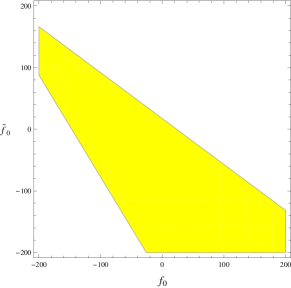
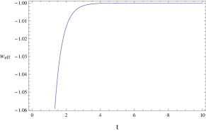
Figure 1: Left region plot shows validity region for WEC and NEC, while Right plot indicates the evolution of effective EoS parameter versus cosmic time. Here $K=1,~{}\omega_{m}=0,~{}\rho_{0}=1$. In right plot, in addition to this, we consider $\tilde{f}_{0}=-2$.

It can be seen that both WEC and NEC remains valid when the free parameters are constrained approximately within these limits: $-25\leq f_{0}\leq 200,~{}88\leq\tilde{f_{0}}\leq 170$. These obtained ranges of free parameters are consistent with the one obtained in 28 . In this case, the effective EoS parameter is given by

$$\omega_{eff}=\frac{\omega_{m}\rho_{0}e^{-3(1+\omega_{m})H_{0}t}+\rho_{0}+\frac{2K}{\kappa^{2}}+\frac{\tilde{f_{0}}e^{T/12H_{0}}}{2\kappa^{2}}}{\rho_{0}e^{-3(1+\omega_{m})H_{0}t}+\rho_{0}-\frac{2K}{\kappa^{2}}-\frac{\tilde{f_{0}}e^{T/12H_{0}}}{2\kappa^{2}}}.$$

Its graphical illustration of $\omega_{eff}$ is given in right plot of Figure 1. It is clear that the effective EoS approaches to $-1$ for late times of the universe.

IV.2 Power law solutions

Here we will investigate the compatibility of WEC and NEC for $f(T,B)$ model reconstructed using power law as expansion factor 28 . Further, we explore the behavior of effective EoS parameter. Let us consider a model described by a power-law scale factor given by

$$a(t)=\left(\frac{t}{t_{0}}\right)^{h},$$

where $t_{0}$ is some fiducial time and $h$ denotes a constant value greater than zero. Such solutions help to explain different phases of cosmic history by taking some specific values of $h$ like matter-matter dominated epoch corresponds to $h=\frac{2}{3}$, while radiation-dominated era relates to $h=\frac{1}{2}$. Also, $h>1$ predicts a late-time accelerating stage of universe. For the above scale factor, the scalar torsion and boundary can be written as follows

$$T=\frac{6h^{2}}{t^{2}},~{}B=\frac{6h(3h-1)}{t^{2}}.$$

By assuming that the ordinary matter contents satisfies the EoS parameter given by $\omega_{m}=\frac{p_{m}}{\rho_{m}}$, we get

$$\rho_{m}=\rho_{0}\left(\frac{t}{t_{0}}\right)^{-3h(1+\omega)},~{}\rho_{m}=\rho_{0}(a(t))^{-3(\omega_{m}+1)},~{}p_{m}=\omega_{m}\rho_{m}.$$

Under all these assumptions, the possible reconstructed form of $f(T,B)$ function describing power-law cosmology is given by

$$f(T,B)=\sqrt{T}C_{1}+B^{\frac{1}{2}(1-3h)}C_{2}+BC_{3}+\frac{2^{1-\frac{3}{2}h(1+\omega_{m})}3^{-\frac{3}{2}h(1+\omega_{m})}\kappa^{2}(\frac{\sqrt{T}t_{0}}{h})^{3h(1+\omega_{m})}\rho_{0}}{1-3h(1+\omega_{m})}.$$ (24)

Introducing Eq.(24) in the energy conditions (19) and (20), we get

$$NEC : \frac{1}{6}H^{4}(1+q)(216+\frac{\sqrt{6}t^{3}C_{1}}{h^{3}}-\frac{2^{-\frac{5}{2}-\frac{3h}{2}}\times 3^{\frac{1}{2}-\frac{3h}{2}}(1+3h)H^{4}(-4+j-3q)\left(\frac{h(-1+3h)}{t^{2}}\right)^{\frac{1}{2}(-1-3h)}t^{2}C_{2}}{h}$$ (25)

$$- \frac{{2^{-\frac{7}{2}-\frac{3h}{2}}}\times 3^{\frac{1}{2}-\frac{3h}{2}}(1+h)(1+3h)H^{6}(-4+j-3q)^{2}\left(\frac{h(-1+3h)}{t^{2}}\right)^{\frac{1}{2}(-1-3h)}t^{6}C_{2}}{(1-3h)^{2}h^{3}}$$

$$-\frac{H^{2}(1+q)(\sqrt{6}tC_{1}+3(-6^{\frac{1}{2}-\frac{3h}{2}}\left(\frac{h(-1+3h)}{t^{2}}\right)^{\frac{1}{2}(1-3h)}t^{2}C_{2}+12hC_{3}))}{6h}\geq 0,$$

$$WEC : \sqrt{6}htC_{1}+6^{\frac{1}{2}-\frac{3h}{2}}\left(\frac{h(-1+3h)}{t^{2}}\right)^{\frac{1}{2}(1-3h)}t^{2}C_{2}$$

$$+ \frac{2^{-\frac{3}{2}(1+h)}\times 3^{\frac{1}{2}-\frac{3h}{2}}(1+3h)H^{4}(-4+j-3q)\left(\frac{h(-1+3h)}{t^{2}}\right)^{\frac{1}{2}(-1-3h)}t^{4}C_{2}}{h}$$

$$+ 6h(-1+3h)C_{3}+3H^{2}(1+q)t^{2}\left(-\frac{6^{-\frac{1}{2}-\frac{3h}{2}}\left(\frac{h(-1+3h)}{t^{2}}\right)^{\frac{1}{2}(1-3h)}t^{2}C_{2}}{h}+2C_{3}\right)\geq 0,~{}\rho_{eff}+p_{eff}\geq 0.$$

These conditions involve parameters like $q,~{}C_{1},~{}C_{2},~{}C_{3},~{}h,~{}j$ and the cosmic time $t$. We explore the validity of these bounds by fixing all other free parameters except $C_{1}$ and also by varying cosmic time. The graphical behavior of these constraints is given in the left panel of Figure 2. Since $h>1$ indicates accelerated expanding late cosmic stages therefore we have chosen values greater than 1. It is seen that by taking greater values of $h$ and $C_{1}$, the validity region of these energy bounds can be extended with increasing cosmic time. Also, it is clear from the graph that for very few negative $C_{1}$ values with small $t$ satisfy these energy bounds.

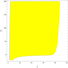
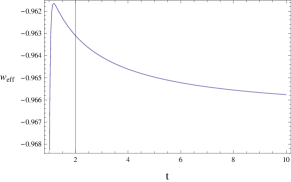
Figure 2: Left panel shows validity region for WEC and NEC while Right plot indicates the evolution of effective EoS parameter versus cosmic time. Here $\omega_{m}=0,~{}t_{0}=\rho_{0}=C_{2}=C_{3}=1$ and $h=10$. Also, in right plot, we take $C_{1}=100$.

Further, the effective EoS parameter in this case is given by

$$\omega_{eff} = \omega_{m}\rho_{m}+\frac{1}{8\pi}[\frac{1}{2}(\sqrt{T}C_{1}+B^{\frac{1}{2}(1-3h)}C_{2}+BC_{3}+\frac{2^{1-\frac{3}{2}h(1+\omega_{m})}3^{-\frac{3}{2}h(1+\omega_{m})}8\pi(\frac{\sqrt{T}t_{0}}{h})^{3h(1+\omega_{m})}\rho_{0}}{1-3h(1+\omega_{m})})$$

$$- \frac{h}{t^{2}}(\frac{C_{1}}{\sqrt{T}}+\frac{2^{2-3/2h(1+\omega_{m})}3^{3/2h(1+\omega_{m})}}{1-3h(1+\omega_{m})}\left(\frac{\sqrt{T}t_{0}}{h}\right)^{3h(\omega_{m}+1)}\frac{t_{0}}{2h\sqrt{T}}-1.5C_{2}(1-3h)B^{1/2(1-3h)-1}-3C_{3})$$

$$- 2\frac{h}{t}({\frac{C_{1}}{4}T^{-\frac{3}{2}}-\frac{2^{2-\frac{3}{2}h(1+\omega_{m})}3^{\frac{3}{2}h(1+\omega_{m})}8\pi\rho_{0}}{(1-3h(1+\omega_{m}))}\frac{3h(1+\omega_{m})}{2}(\frac{t_{0}}{h})^{3h(1+\omega_{m})}(\frac{3}{2}h(1+\omega_{m})-1)T^{\frac{3}{2}h(1+\omega_{m})-2}}(\frac{12h^{2}}{t^{3}}))$$

$$- 9(\frac{h}{t})^{2}(\frac{1}{2}C_{2}(1-3h)B^{\frac{1}{2}(1-3h)-1}+C_{3})+(\frac{1}{2}(1-3h)(\frac{1}{2}(1-3h)-1)(\frac{1}{2}(1-3h)-2)C_{2}B^{\frac{1}{2}(1-3h)-3})$$

$$\times (-\frac{12h(3h-1)}{t^{3}})^{2}+(\frac{1}{2}(1-3h)(\frac{1}{2}(1-3h)-1)C_{2}B^{\frac{1}{2}(1-3h)-2})(\frac{36h(3h-1)}{t^{4}})]$$

$$\times [\rho_{m}+\frac{1}{8\pi}\{\frac{3h}{2t}(1-3h)(\frac{1}{2}(1-3h)-1)C_{2}B^{\frac{1}{2}(1-3h)-2)\frac{12h(3h-1)}{t^{2}}}+(-\frac{3h}{t^{2}}+\frac{9h^{2}}{t^{2}})$$

$$\times (\frac{C_{2}}{2}(1-3h)B^{\frac{1}{2}(1-3h)-1)}+C_{3})-\frac{1}{2}(\sqrt{T}C_{1}+B^{\frac{1}{2}(1-3h)}C_{2}+BC_{3}$$

$$+ \frac{2^{1-\frac{3}{2}h(1+\omega_{m})}3^{-\frac{3}{2}h(1+\omega_{m})}8\pi(\frac{\sqrt{T}t_{0}}{h})^{3h(1+\omega_{m})}\rho_{0}}{1-3h(1+\omega_{m})}))\}]^{-1}.$$

The evolution of this parameter is given in the right panel of Figure 2. Clearly $-1\leq\omega_{eff}\leq 0$ represents the accelerated expanding stages of cosmic evolution.

IV.3 $\Lambda$CDM Cosmology

In this section, we will use the reconstructed $f(T,B)$ function for a $\Lambda CDM$ cosmological evolution without including any cosmological constant term in this modified gravity. For this purpose, we take $f(T,B)$ as obtained in 28

$$f(T,B)=BC_{1}+C_{1}\sqrt{T}+\frac{C_{2}}{\sqrt{B}}-\frac{2^{-\omega_{m}}\kappa^{2}\rho_{0}}{2\omega_{m}+1}\left(\frac{T}{3a_{0}^{3}l}\right)^{\omega_{m}+1}.$$ (28)

Introducing Eq.(28) in the energy conditions (19) and (20), we get

$$NEC : 93312H^{5}(1+q)-15552H^{3}(1+q)C_{1}+\sqrt{2}(64+22j-5j^{2}+6q+30jq-45q^{2})C_{2}\geq 0,$$

$$WEC : 72H^{2}\left(\sqrt{6}+6H(4+q)\right)C_{1}+\sqrt{2}\left(6+j-5q\right)C_{2}\geq 0.$$

Here $a(t)=a_{0}e^{N},~{}H^{2}=g=le^{-3N},~{}l=\frac{8\pi}{3}$. Further, the torsion scalar and boundary terms turn out to be $T=6le^{-3N}$ and $B=9le^{-3N}$. It is worthwhile to mention here that $N=-\ln(1+z)$ is called e-folding parameter and $z$ is called redshift function. It further yields the relationship: $a(t)=\frac{a_{0}}{1+z}$. The graphical illustration of these energy bounds in terms of validity region is given by left panel of Figure 3. Clearly, these constraints are satisfied for positive $C_{1}$ values only. It can also be seen that there are few values $C_{1}>50$ with small values of red shift function (large values of scale factor), where these constraints are no longer valid.

Also, the effective EoS parameter is given by

$$\omega_{eff} = [\omega_{m}\rho_{m}+\frac{1}{8\pi}\{\frac{1}{2}(BC_{1}+C_{1}\sqrt{T}+\frac{C_{2}}{\sqrt{B}}-\frac{2^{-\omega}\kappa^{2}\rho_{0}}{2\omega+1}\left(\frac{T}{3a_{0}^{3}l}\right)^{\omega+1})-\frac{3}{2}le^{-3N}(2(\frac{C_{3}}{2\sqrt{T}}$$

$$- \frac{2^{-\omega}8\pi\rho_{0}}{2\omega_{m}+1}(\omega_{m}+1)\frac{1}{3a_{0}^{3}l}\left(\frac{T}{3a_{0}^{3}l}\right)^{\omega_{m}})-3(C_{1}-\frac{C_{2}}{2B^{\frac{3}{2}}}))-2H((-\frac{C_{3}}{4T^{\frac{3}{2}}}$$

$$- \frac{2^{-\omega}8\pi\rho_{0}\omega_{m}}{2\omega_{m}+1}(\omega_{m}+1)\frac{1}{(3a_{0}^{3}l)^{2}}\left(\frac{T}{3a_{0}^{3}l}\right)^{\omega_{m}-1})H(-18le^{-3N}))-9H^{2}(C_{1}-\frac{C_{2}}{2B^{\frac{3}{2}}})$$

$$- \frac{243}{4}C_{2}l^{-1}He^{3N}\}][\rho_{m}+\frac{1}{8\pi}\{3H(\frac{81}{4}C_{2}lHB^{-\frac{5}{2}}e^{-3N})+(-3\frac{3}{2}le^{-3N}+9le^{-3N})$$

$$- \frac{1}{2}(BC_{1}+C_{1}\sqrt{T}+\frac{C_{2}}{\sqrt{B}}-\frac{2^{-\omega}\kappa^{2}\rho_{0}}{2\omega+1}\left(\frac{T}{3a_{0}^{3}l}\right)^{\omega+1})\}]^{-1}.$$

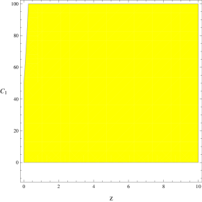
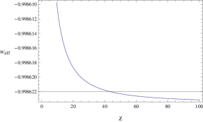
Figure 3: Left region plot shows validity region for WEC and NEC while Right plot indicates the evolution of effective EoS parameter versus cosmic time. For left graph, we consider $q=-.64,~{}j=1.02,~{}l=\frac{8\pi}{3}$ and $C_{2}=10$. For right plot, we take $\omega_{m}=0,~{}a_{0}=1=\rho_{0},~{}C_{1}=1000,~{}C_{2}=C_{3}=10$.

The dynamics of effective EoS parameter is provided in the right penal of Figure 3. It indicates that the universe model is in quintessence stage of its evolution.

IV.4 Phantom Universe Model

In this section, we will discuss the evolution of energy condition bounds for reconstructed phantom model of universe 28 . This phantom universe model is given by

$$f(T,B)=C_{1}B^{\frac{3+m}{2m}}+C_{2}B+16\pi b_{0}+C_{3}\sqrt{T}-\frac{8\pi b_{1}T}{3h_{0}^{2}}-\frac{\sqrt{8\pi\frac{8}{3}}b_{2}(m+1)T^{\frac{5}{2}}}{15h_{0}^{5}},$$ (29)

where $C_{1},~{}C_{2},~{}C_{3},~{}b_{0},~{}b_{1},~{}m$ and $h_{0}$ are all constants. Here the ordinary energy density and Hubble parameter are given by $\rho_{m}=b_{0}+b_{1}e^{2mN}+\frac{96(m+1)}{5}b_{2}e^{5mN};~{}m\neq-3$ and $H=\sqrt{g}=h_{0}e^{mN}$, respectively. Further $N=\ln(\frac{1}{1+z})$ and is called e-folding parameter and $z$ is the red shift parameter. For this model (29), the WEC (19) and NEC (20) are given by

$$8\pi(1+\omega_{m})\left(b_{0}+b_{1}e^{2mN}+\frac{96(m+1)}{5}b_{2}e^{5mN}\right)-h_{0}^{2}e^{2mN}(1+q)\{3\left(C_{2}+C_{1}(\frac{3+m}{2m})B^{\frac{3-m}{2m}}\right)$$

$$+\frac{C_{3}}{2\sqrt{T}}-\frac{8b_{1}\pi}{3h_{0}^{2}}-\frac{\sqrt{8\pi\frac{8}{3}}b_{2}(m+1)\frac{5}{2}T^{\frac{3}{2}}}{15h_{0}^{5}}\}-18h_{0}^{4}e^{4mN}(j-3q-4)\left(\frac{9-m^{2}}{4m^{2}}\right)C_{1}B^{\frac{3(1-m)}{2m}}$$

$$+36h_{0}^{4}e^{4mN}(1+q)-24h_{0}^{4}e^{4mN}(1+q)\{-\frac{C_{3}}{4}T^{-\frac{3}{2}}-\frac{\sqrt{8\pi\frac{8}{3}}b_{2}(m+1)T^{\frac{1}{2}}}{4h_{0}^{5}}\}+36h_{0}^{4}e^{4mN}(j-3q-4)^{2}$$

$$\times\{\frac{3(1-m)(9-m^{2})}{8m^{3}}C_{1}B^{\frac{3-5m}{2m}}\}\}\geq 0,$$ (30)

$$8\pi\left(b_{0}+b_{1}e^{2mN}+\frac{96(m+1)}{5}b_{2}e^{5mN}\right)-18h_{0}^{4}e^{4mN}(j-3q-4)\left(\frac{9-m^{2}}{4m^{2}}\right)C_{1}B^{\frac{3(1-m)}{2m}}$$

$$-3h_{0}^{2}e^{2mN}(1+q)\left(C_{2}+C_{1}B^{\frac{3-m}{2m}}\frac{3+m}{2m}\right)-\frac{1}{2}\{C_{1}B^{\frac{3+m}{2m}}+C_{2}B+16\pi b_{0}+C_{3}\sqrt{T}-\frac{8\pi b_{1}T}{3h_{0}^{2}}$$

$$-\frac{\sqrt{8\pi\frac{8}{3}}b_{2}(m+1)T^{\frac{5}{2}}}{15h_{0}^{5}}\}\geq 0.$$ (31)

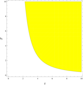
Figure 4: Left region plot shows validity region for WEC and NEC while Right plot indicates the evolution of effective EoS parameter versus cosmic time. For right plot, we assume $h_{0}=-0.1,~{}\omega_{m}=0,~{}m=2,~{}j=1.02,~{}q=-1,~{}b_{0}=1,~{}b_{1}=2,~{}b_{2}=0.0001$ and $C_{1}=C_{2}=C_{3}=1.$

The graphical illustration of these energy bounds versus red shift parameter and constant $b_{0}$ are given in Figure 4. Furthermore, the effective EoS parameter turns out to be

$$\omega_{eff} = [\omega_{m}\rho_{m}+\frac{1}{8\pi}\{\frac{1}{2}(C_{1}B^{\frac{3+m}{2m}}+C_{2}B+16\pi b_{0}+C_{3}\sqrt{T}-\frac{8\pi b_{1}T}{3h_{0}^{2}}-\frac{\sqrt{8\pi\frac{8}{3}}b_{2}(m+1)T^{\frac{5}{2}}}{15h_{0}^{5}})$$

$$+ mh_{0}^{2}e^{2mN}(2(\frac{C_{3}}{2\sqrt{T}}-\frac{8\sqrt{\frac{8}{3}}\pi b_{2}(m+1)}{15h_{0}^{5}}\frac{5}{2}T^{\frac{3}{2}})-3(C_{1}\left(\frac{3+m}{2m}\right)B^{\frac{3+m}{2m}-1}+C_{2}))$$

$$- 2h_{0}e^{mN}(12mh_{0}^{3}e^{3mN}\left(-\frac{C_{3}}{4T^{\frac{3}{2}}}-\frac{1}{6h_{0}^{5}}\sqrt{\frac{8}{3}}8\pi b_{2}(m+1)\frac{3}{2}T^{\frac{1}{2}}\right))-9h_{0}^{2}e^{2mN}(h_{0}e^{mN}$$

$$\times \left(C_{1}\frac{9-m^{2}}{4m^{2}}B^{\frac{3(1-m)}{2m}}\right)\left(6h_{0}^{2}(m+1)e^{2mN}\right))+C_{1}\frac{9-m^{2}}{4m^{2}}(m+1)6h_{0}^{4}e^{mN}$$

$$\times \left(\frac{3(1-m)}{2m}B^{\frac{3(1-m)}{2m}-1}(6h_{0}^{2}(m+1)e^{4mN})+2me^{2mN}B^{\frac{3(1-m)}{2m}}\right)\}][\rho_{m}+\frac{1}{8\pi}\{-3h_{0}e^{mN}(h_{0}e^{mN}$$

$$\times \left(C_{1}\frac{9-m^{2}}{4m^{2}}B^{\frac{3(1-m)}{2m}}\right)\left(6h_{0}^{2}(m+1)e^{2mN}\right))+(3mh_{0}^{2}e^{2mN}+9h_{0}^{2}e^{2mN})(C_{1}\left(\frac{3+m}{2m}\right)B^{\frac{3+m}{2m}-1}$$ (32)

$$+ C_{2})-\frac{1}{2}(C_{1}B^{\frac{3+m}{2m}}+C_{2}B+16\pi b_{0}+C_{3}\sqrt{T}-\frac{8\pi b_{1}T}{3h_{0}^{2}}-\frac{\sqrt{8\pi\frac{8}{3}}b_{2}(m+1)T^{\frac{5}{2}}}{15h_{0}^{5}})\}]^{-1}.$$

The possible validity of energy constraints and the dynamics of the effective EoS parameter is illustrated in the Figure 4. In the left penal, the validity region of NEC and WEC is given for the described choice of free parameters. It is shown that the energy constraints are valid for increasing values of $b_{0}$ and redshift $z$, in particular, $z\geq 3$ (decreasing rate of scale factor). For very small values of $b_{0}$ closer to zero, these constraints remain invalid. The EoS parameter indicates the negative behavior as shown in the right penal.

V Evolution of Energy Bounds using Reconstructed Models for $f(T,B)=-T+F(B)$ cosmology

In this section, we will study the specific case where the function takes the form $f(T,B)=-T+F(B)$, which is similar to models of the form $f(R)=R+F(R)$ and $f(T)=-T+f(T)$ studied in $f(R)$ and $f(T)$ gravity, respectively. This theory is equivalent than to consider a teleparallel background (or $GR$) plus an additional function which depends on the boundary term which can be also understood as $F(B)=F(T+R)$. Using $f(T,B)=-T+F(B)$ in the energy conditions (19) and (20), we get this specific form of energy conditions:

$$NEC : 36H^{4}(1+q)+\kappa^{2}(p_{m}+\rho_{m})-2H^{2}(1+q)(-1+3F_{B})-18H^{4}(-4+j-3q)F_{BB}$$ (33)

$$+ 36H^{6}(-4+j-3q)^{2}F_{BBB}\geq 0,$$

$$WEC : \frac{1}{2}(T-F(B))+\kappa^{2}\rho_{m}-3H^{2}(1+q)F_{B}-18H^{4}(-4+j-3q)F_{BB}\geq 0.$$ (34)

Similar to the previous section, now we will check the evolution of energy condition bounds as well as EoS parameter for previously mentioned four specific cases.

For a de-Sitter reconstruction, the scale factor behaves as $a(t)=a_{0}e^{H_{o}t}$, then $B=18H_{0}^{2}$ and hence we consider $F(B)$ as

$$F(B)=C_{1}e^{\frac{B}{18H_{o}^{2}}}-2(3H_{0}^{2}-\kappa^{2}\rho_{0}).$$ (35)

Here $C_{1}$ is an integration constant. Using (35) in (33) and (34), we get

$$NEC : 324H_{0}^{2}(1+18H_{0}^{2})(1+q)+e(-2+j^{2}-3q+9q^{2}-j(17+6q))C_{1}\geq 0$$ (36)

$$WEC : 108H_{0}^{2}-e(8+j)C_{1}\geq 0$$ (37)

These constraints involve parameters $H_{0},~{}q,~{}j$ and $C_{1}$. The consistency of these energy bounds for $q$ parameter and $C_{1}$ is shown in left plot of Figure 5. Clearly, it indicates that these energy bounds will remain valid if $C_{1}$ is negative while $-1\leq q\leq 2$ that corresponds to quintessence, radiation, matter and dust dominated cosmic epochs. Thus it can be concluded that in phantom cosmic phase, these bounds will not be consistent. Also, the effective EoS parameter, in this case, takes the following form:

$$\omega_{eff}=\frac{\omega_{m}\rho_{0}e^{-3(1+\omega_{m})H_{0}t}-\frac{1}{\kappa^{2}}(6H_{0}^{2}+\kappa^{2}\rho_{0})}{\rho_{0}e^{-3(1+\omega_{m})H_{0}t}+\frac{1}{\kappa^{2}}(6H_{0}^{2}-\kappa^{2}\rho_{0})}.$$ (38)

The right plot of Figure 5 represents the behavior of this parameter versus cosmic time. Clearly, its negative values less than -1 corresponds to the phantom stage of cosmic evolution.

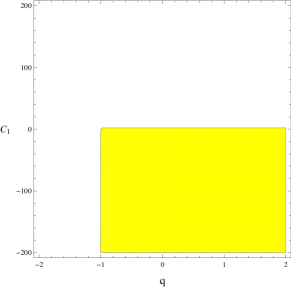
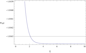
Figure 5: Left region plot shows validity region for WEC and NEC while Right plot indicates the evolution of effective EoS parameter versus cosmic time. For left plot, $H_{0}=0.718$ and $j=1.02$. For right plot, we assume $\rho_{0}=0.001$ and $\omega_{m}=0$.

For a power-law cosmology, we take $F(B)$ in the following form:

$$F(B) = C_{1}B^{\frac{1-3h}{2}}+B\left(C_{2}-\frac{2h}{(3h+1)^{2}}\right)+\frac{hBLog(B)}{3h+1}+\frac{BhLog(9h+3)}{3h+1}$$ (39)

$$- \frac{\kappa^{2}\rho_{0}\left((3h-1)^{1-\frac{3}{2}h(\omega_{m}+1)}\times 2^{2-\frac{3}{2}h(\omega_{m}+1)}\right)\left(\frac{Bt_{0}^{2}}{3h}\right)^{\frac{3}{2}h(\omega_{m}+1)}}{\left(3h(\omega_{m}+1)-2\right)\left(3h(\omega_{m}+2)-1\right)},$$

where $C_{1}$ and $C_{2}$ are integration constants. Using (39) in (33) and (34), we get

$$NEC : 36H^{4}(1+q)+\frac{H^{6}(-4+j-3q)^{2}t^{4}}{12h^{3}(-1+3h)^{3}}\left(-\frac{12h^{2}(-1+3h)}{1+3h}-2^{-\frac{3}{2}(1+h)}\times 3^{-\frac{3}{2}(-1+h)}(1+h)(9h^{2}-1)\right.$$ (40)

$$\left.\times\left(\frac{h(-1+3h)}{t^{2}}\right)^{\frac{1}{2}(1-3h)}t^{2}C_{1}\right)-\frac{H^{4}(-4+j-3q)t^{2}\left(\frac{12(-1+3h)}{1+3h}+\frac{6^{\frac{1}{2}-\frac{3h}{2}}(-1+\frac{1}{2}(1-3h))(1-3h)\left(\frac{h(-1+3h)}{t^{2}}\right)^{\frac{1}{2}-\frac{3h}{2}}t^{2}C_{1}}{h^{2}}\right)}{4(1-3h)^{2}}$$

$$-2H^{2}(1+q)\Bigg{[}-1+\frac{3}{2}\Bigg{[}-\frac{6^{-\frac{1}{2}-\frac{3h}{2}}\left(\frac{h(-1+3h)}{t^{2}}\right)^{\frac{1}{2}(1-3h)}t^{2}C_{1}}{h}$$

$$+\frac{2(h(-1+3h+(1+3h)Log(3+9h)+(1+3h)Log(\frac{6h(-1+3h)}{t^{2}}))+(1+3h)^{2}C_{2})}{(1+3h)^{2}}\Bigg{]}\Bigg{]}\geq 0$$

$$WEC : \frac{1}{ht^{2}}\Bigg{[}-2^{-\frac{1}{2}-\frac{3h}{2}}\times 3^{\frac{1}{2}-\frac{3h}{2}}\left(\frac{h(-1+3h)}{t^{2}}\right)^{\frac{1}{2}(-1-3h)}\left(4h^{2}(-1+3h)-2h(-1+3h)H^{2}(1+q)t^{2}\right.$$ (41)

$$\left.+(1+3h)H^{4}(-4+j-3q)t^{4}\right)C_{1}\Bigg{]}+\frac{12}{(-1+3h)(t+3ht)^{2}}\Bigg{[}h^{2}(-1+3h)(-1+3h(4+3h))$$

$$-(1-3h)^{2}hH^{2}(1+q)t^{2}+(1+3h)H^{4}(4-j+3q)t^{4}-h(-1+9h^{2})(h(-1+3h)+H^{2}(1+q)t^{2})$$

$$\left(Log(3+9h)+Log\left(\frac{6h(-1+3h)}{t^{2}}\right)-(-1+3h)(1+3h)^{2}\left(h(-1+3h)+H^{2}(1+q)t^{2}\right)C_{2}\right)\Bigg{]}\geq 0$$

Also, effective EoS parameter can be written as

$$\omega_{eff} = [\omega_{m}\rho_{m}+\frac{1}{8\pi}\{\frac{1}{2}(-T+C_{1}B^{\frac{1-3h}{2}}+B\left(C_{2}-\frac{2h}{(3h+1)^{2}}\right)+\frac{h}{3h+1}B\log(B)+\frac{h\log(9h+3)}{3h+1}B$$

$$- \frac{8\pi\left((3h-1)^{1-\frac{3}{2}h(\omega_{m}+1)}2^{2-\frac{3}{2}h(\omega_{m}+1)}\right)}{(3h(\omega_{m}+1)-2)(3h(\omega_{m}+2)-1)}(\frac{Bt_{0}^{2}}{3h})^{\frac{3}{2}h(\omega_{m}+1)})+\frac{h}{t^{2}}(2+3(C_{1}\frac{1-3h}{2}B^{\frac{1-3h}{2}-1}$$

$$+ \left(C_{2}-\frac{2h}{(3h+1)^{2}}\right)-\frac{h}{3h+1}\left(\log(B)+\frac{1}{\ln(10)}\right)+\frac{h\log(9h+3)}{3h+1}$$

$$- \frac{8\pi\left((3h-1)^{1-\frac{3}{2}h(\omega_{m}+1)}2^{2-\frac{3}{2}h(\omega_{m}+1)}\right)}{(3h(\omega_{m}+1)-2)(3h(\omega_{m}+2)-1)}(\frac{t_{0}^{2}}{3h})^{\frac{3}{2}h(\omega_{m}+1)}(\frac{3}{2}h(\omega_{m}+1))B^{\frac{3}{2}h(\omega_{m}+1)-1}))$$

$$- 9(\frac{h}{t})^{2}(C_{1}\frac{1-3h}{2}B^{\frac{1-3h}{2}-1}+\left(C_{2}-\frac{2h}{(3h+1)^{2}}\right)-\frac{h}{3h+1}\left(\log(B)+\frac{1}{\ln(10)}\right)+\frac{h\log(9h+3)}{3h+1}$$

$$- \frac{8\pi\left((3h-1)^{1-\frac{3}{2}h(\omega_{m}+1)}2^{2-\frac{3}{2}h(\omega_{m}+1)}\right)}{(3h(\omega_{m}+1)-2)(3h(\omega_{m}+2)-1)}(\frac{t_{0}^{2}}{3h})^{\frac{3}{2}h(\omega_{m}+1)}(\frac{3}{2}h(\omega_{m}+1))B^{\frac{3}{2}h(\omega_{m}+1)-1})$$

$$+ \left(-\frac{12h(3h-1)}{t^{3}}\right)^{2}\{C_{1}\frac{9h^{2}-1}{4}(\frac{1-3h}{2}-2)B^{\frac{1-3h}{2}-3}+\frac{h}{3h+1}\left(\frac{1}{B^{2}\ln(10)}\right)$$

$$- \frac{8\pi\left((3h-1)^{1-\frac{3}{2}h(\omega_{m}+1)}2^{2-\frac{3}{2}h(\omega_{m}+1)}\right)}{(3h(\omega_{m}+1)-2)(3h(\omega_{m}+2)-1)}(\frac{t_{0}^{2}}{3h})^{\frac{3}{2}h(\omega_{m}+1)}(\frac{3}{2}h(\omega_{m}+1))(\frac{3}{2}h(\omega_{m}+1)-1)$$

$$\times (\frac{3}{2}h(\omega_{m}+1)-2)B^{\frac{3}{2}h(\omega_{m}+1)-3}\}+\{C_{1}\frac{9h^{2}-1}{4}B^{\frac{1-3h}{2}-2}-\frac{h}{3h+1}\left(\frac{1}{B\ln(10)}\right)$$

$$- \frac{8\pi\left((3h-1)^{1-\frac{3}{2}h(\omega_{m}+1)}2^{2-\frac{3}{2}h(\omega_{m}+1)}\right)}{(3h(\omega_{m}+1)-2)(3h(\omega_{m}+2)-1)}(\frac{t_{0}^{2}}{3h})^{\frac{3}{2}h(\omega_{m}+1)}(\frac{3}{2}h(\omega_{m}+1))(\frac{3}{2}h(\omega_{m}+1)-1)$$

$$\times B^{\frac{3}{2}h(\omega_{m}+1)-2}\}\left(\frac{36h(3h-1)}{t^{4}}\right)\}][\rho_{m}+\frac{1}{8\pi}\{-3\frac{h}{t}(\left(-\frac{12h(3h-1)}{t^{3}}\right)\{C_{1}\frac{9h^{2}-1}{4}B^{\frac{1-3h}{2}-2}$$

$$- \frac{h}{3h+1}\left(\frac{1}{B\ln(10)}\right)-\frac{8\pi\left((3h-1)^{1-\frac{3}{2}h(\omega_{m}+1)}2^{2-\frac{3}{2}h(\omega_{m}+1)}\right)}{(3h(\omega_{m}+1)-2)(3h(\omega_{m}+2)-1)}(\frac{t_{0}^{2}}{3h})^{\frac{3}{2}h(\omega_{m}+1)}(\frac{3}{2}h(\omega_{m}+1))$$

$$\times (\frac{3}{2}h(\omega_{m}+1)-1)B^{\frac{3}{2}h(\omega_{m}+1)-2}\})+\left(\frac{9h^{2}}{t^{2}}-\frac{3h}{t^{2}}\right)(\left(-\frac{12h(3h-1)}{t^{3}}\right)\{C_{1}\frac{9h^{2}-1}{4}B^{\frac{1-3h}{2}-2}$$

$$- \frac{h}{3h+1}\left(\frac{1}{B\ln(10)}\right)-\frac{8\pi\left((3h-1)^{1-\frac{3}{2}h(\omega_{m}+1)}2^{2-\frac{3}{2}h(\omega_{m}+1)}\right)}{(3h(\omega_{m}+1)-2)(3h(\omega_{m}+2)-1)}(\frac{t_{0}^{2}}{3h})^{\frac{3}{2}h(\omega_{m}+1)}(\frac{3}{2}h(\omega_{m}+1))$$

$$\times (\frac{3}{2}h(\omega_{m}+1)-1)B^{\frac{3}{2}h(\omega_{m}+1)-2}\})-\frac{1}{2}(-T+C_{1}\frac{1-3h}{2}B^{\frac{1-3h}{2}-1}+\left(C_{2}-\frac{2h}{(3h+1)^{2}}\right)$$

$$- \frac{h}{3h+1}\left(\log(B)+\frac{1}{\ln(10)}\right)+\frac{h\log(9h+3)}{3h+1}-\frac{8\pi\left((3h-1)^{1-\frac{3}{2}h(\omega_{m}+1)}2^{2-\frac{3}{2}h(\omega_{m}+1)}\right)}{(3h(\omega_{m}+1)-2)(3h(\omega_{m}+2)-1)}$$

$$\times (\frac{t_{0}^{2}}{3h})^{\frac{3}{2}h(\omega_{m}+1)}(\frac{3}{2}h(\omega_{m}+1))B^{\frac{3}{2}h(\omega_{m}+1)-1})\}]^{-1}.$$

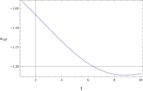
Figure 6: Left region plot shows validity region for WEC and NEC while Right plot indicates the evolution of effective EoS parameter versus cosmic time. Here $\rho_{0}=t_{0}=C_{2}=C_{3}=1$ and $\omega_{m}=0,~{}h=10$. For right plot, $C_{1}=10$.

The graphical illustration for energy constraints and effective EoS parameter is presented in the Figure 6. The left penal provides the possible validity region for energy bounds. It is found that for initial cosmic time, these constraints are valid with $-100\leq C_{1}\leq 100$. Further, these constraints are also valid if $C_{1}\leq 0$ and $30\leq t\leq 50$. The right penal indicates the dynamics of EoS parameter versus cosmic time. Its negative behavior less than -1 corresponds to phantom accelerated phase of cosmos.

For $\Lambda CDM$ Universe, we choose $F(B)$ as

$$F(B)=BC_{1}+\frac{log(B-18H_{0}^{2})(6a_{0}^{3}Bl-2B\kappa^{2}\rho_{0})+6a_{0}^{3}l(B-9H_{0}^{2})+\kappa^{2}\rho_{0}(B-36H_{0}^{2})}{27a_{0}^{3}l}$$

$$+\frac{C_{2}\left(3H_{0}\sqrt{B-9H_{0}^{2}}-B\times arctan\left(\frac{\sqrt{B-9H_{0}^{2}}}{3H_{0}}\right)\right)}{54H_{0}^{3}}.$$ (42)

The corresponding weak and null energy condition bounds are given by

$$36(\sqrt{H_{0}^{2}+le^{-3N}})^{4}(1+q)+8\pi\rho_{0}(1+\omega_{m})\left(\frac{a_{0}}{1+z}\right)^{-3(\omega_{m}+1)}-2(H_{0}^{2}+le^{-3N})(1+q)(-1+3\{C_{1}$$ (43)

$$+\frac{1}{27a_{0}^{3}l}\left(\frac{B(6a_{0}^{3}l-16\pi\rho_{0})}{\ln(10)(B-18H_{0}^{2})}+\log(B-18H_{0}^{2})(6a_{0}^{3}l-16\pi\rho_{0})+6a_{0}^{3}l+8\pi\rho_{0}\right)-\frac{C_{2}}{54H_{0}^{3}}\arctan\left(\frac{\sqrt{B-9H_{0}^{2}}}{3H_{0}}\right)\})$$

$$-18H_{0}^{2}(H_{0}^{2}+le^{-3N})^{2}(-4+j-3q)(\frac{1}{27a_{0}^{3}l}\left(\frac{(6a_{0}^{3}l-16\pi\rho_{0})}{\ln(10)}\left(\frac{1}{B-18H_{0}^{2}}-\frac{B}{(B-18H_{0}^{2})^{2}}\right)+\frac{(6a_{0}^{3}l-16\pi\rho_{0})}{\ln(10)(B-18H_{0}^{2})}\right)$$

$$-\frac{3C_{2}}{108H_{0}^{2}}B^{-1}(B-9H_{0}^{2})^{-\frac{1}{2}})+36(H_{0}^{2}+le^{-3N})(-4+j-3q)^{2}(\frac{1}{27a_{0}^{3}l}$$

$$\times \left(\frac{(6a_{0}^{3}l-16\pi\rho_{0})}{\ln(10)}\left(-\frac{2}{(B-18H_{0}^{2})^{2}}+\frac{2B}{(B-18H_{0}^{2})^{3}}\right)-\frac{(6a_{0}^{3}l-16\pi\rho_{0})}{\ln(10)(B-18H_{0}^{2})^{2}}\right)$$

$$+ \frac{C_{2}}{12H_{0}}\left(B^{-2}(B-9H_{0}^{2})^{-\frac{1}{2}}+B^{-1}\frac{1}{2}(B-9H_{0}^{2})^{-\frac{3}{2}}\right))\geq 0,$$

$$\frac{1}{2}\{6le^{-3N}+6H_{0}^{2}-(BC_{1}+\frac{log(B-18H_{0}^{2})(6a_{0}^{3}Bl-2B\kappa^{2}\rho_{0})+6a_{0}^{3}l(B-9H_{0}^{2})+\kappa^{2}\rho_{0}(B-36H_{0}^{2})}{27a_{0}^{3}l}$$

$$+\frac{C_{2}\left(3H_{0}\sqrt{B-9H_{0}^{2}}-B\times arctan\left(\frac{\sqrt{B-9H_{0}^{2}}}{3H_{0}}\right)\right)}{54H_{0}^{3}})\}+8\pi\rho_{0}\left(\frac{a_{0}}{1+z}\right)^{-3(1+\omega_{m})}$$

$$-3(H_{0}^{2}+le^{-3N})(1+q)(C_{1}+\frac{1}{27a_{0}^{3}l}\left(\frac{B(6a_{0}^{3}l-16\pi\rho_{0})}{\ln(10)(B-18H_{0}^{2})}+\log(B-18H_{0}^{2})(6a_{0}^{3}l-16\pi\rho_{0})+6a_{0}^{3}l+8\pi\rho_{0}\right)$$

$$-\frac{C_{2}}{54H_{0}^{3}}\arctan\left(\frac{\sqrt{B-9H_{0}^{2}}}{3H_{0}}\right))-18(H_{0}^{2}+le^{-3N})^{2}(-4+j-3q)$$

$$\times(\frac{1}{27a_{0}^{3}l}\left(\frac{(6a_{0}^{3}l-16\pi\rho_{0})}{\ln(10)}\left(\frac{1}{B-18H_{0}^{2}}-\frac{B}{(B-18H_{0}^{2})^{2}}\right)+\frac{(6a_{0}^{3}l-16\pi\rho_{0})}{\ln(10)(B-18H_{0}^{2})}\right)$$

$$-\frac{3C_{2}}{108H_{0}^{2}}B^{-1}(B-9H_{0}^{2})^{-\frac{1}{2}})\geq 0.$$

The corresponding effective EoS parameter is given by

$$\omega_{eff} = [\omega_{m}\rho_{m}+\frac{1}{8\pi}\{\frac{1}{2}(-T+BC_{1}+\frac{log(B-18H_{0}^{2})(6a_{0}^{3}Bl-16\pi B\rho_{0})+6a_{0}^{3}l(B-9H_{0}^{2})+8\pi\rho_{0}(B-36H_{0}^{2})}{27a_{0}^{3}l}$$ (44)

$$+ \frac{C_{2}\left(3H_{0}\sqrt{B-9H_{0}^{2}}-B\times arctan\left(\frac{\sqrt{B-9H_{0}^{2}}}{3H_{0}}\right)\right)}{54H_{0}^{3}})+\frac{3}{2}le^{-3N}(2+3(C_{1}$$

$$+ \frac{1}{27a_{0}^{3}l}\left(\frac{B(6a_{0}^{3}l-16\pi\rho_{0})}{\ln(10)(B-18H_{0}^{2})}+\log(B-18H_{0}^{2})(6a_{0}^{3}l-16\pi\rho_{0})+6a_{0}^{3}l+8\pi\rho_{0}\right)$$

$$- \frac{C_{2}}{54H_{0}^{3}}\arctan\left(\frac{\sqrt{B-9H_{0}^{2}}}{3H_{0}}\right)))-9H^{2}(C_{1}+\frac{1}{27a_{0}^{3}l}\{\frac{B(6a_{0}^{3}l-16\pi\rho_{0})}{\ln(10)(B-18H_{0}^{2})}+\log(B-18H_{0}^{2})(6a_{0}^{3}l$$

$$- 16\pi\rho_{0})+6a_{0}^{3}l+8\pi\rho_{0}\}-\frac{C_{2}}{54H_{0}^{3}}\arctan\left(\frac{\sqrt{B-9H_{0}^{2}}}{3H_{0}}\right))+(H_{0}^{2}+le^{-3N})^{\frac{1}{2}}((-27le^{-3N})^{2}(\frac{1}{27a_{0}^{3}l}$$

$$\times \left(\frac{(6a_{0}^{3}l-16\pi\rho_{0})}{\ln(10)}\left(-\frac{2}{(B-18H_{0}^{2})^{2}}+\frac{2B}{(B-18H_{0}^{2})^{3}}\right)-\frac{(6a_{0}^{3}l-16\pi\rho_{0})}{\ln(10)(B-18H_{0}^{2})^{2}}\right)$$

$$+ \frac{C_{2}}{12H_{0}}\left(B^{-2}(B-9H_{0}^{2})^{-\frac{1}{2}}+B^{-1}\frac{1}{2}(B-9H_{0}^{2})^{-\frac{3}{2}}\right))+(81le^{-3N})(\frac{1}{27a_{0}^{3}l}\{\frac{(6a_{0}^{3}l-16\pi\rho_{0})}{\ln(10)}$$

$$\times \left(\frac{1}{B-18H_{0}^{2}}-\frac{B}{(B-18H_{0}^{2})^{2}}\right)+\frac{(6a_{0}^{3}l-16\pi\rho_{0})}{\ln(10)(B-18H_{0}^{2})}\}-\frac{3C_{2}}{108H_{0}^{2}}B^{-1}(B-9H_{0}^{2})^{-\frac{1}{2}}))\}]$$

$$\times [\rho_{m}+\frac{1}{8\pi}\{3(H_{0}^{2}+le^{-3N})(27le^{-3N})(\frac{1}{27a_{0}^{3}l}\{\frac{(6a_{0}^{3}l-16\pi\rho_{0})}{\ln(10)}\left(\frac{1}{B-18H_{0}^{2}}-\frac{B}{(B-18H_{0}^{2})^{2}}\right)$$

$$+ \frac{(6a_{0}^{3}l-16\pi\rho_{0})}{\ln(10)(B-18H_{0}^{2})}\}-\frac{3C_{2}}{108H_{0}^{2}}B^{-1}(B-9H_{0}^{2})^{-\frac{1}{2}})+(-\frac{9}{2}le^{-3N}+9(H_{0}^{2}+le^{-3N}))(C_{1}$$

$$+ \frac{1}{27a_{0}^{3}l}\left(\frac{B(6a_{0}^{3}l-16\pi\rho_{0})}{\ln(10)(B-18H_{0}^{2})}+\log(B-18H_{0}^{2})(6a_{0}^{3}l-16\pi\rho_{0})+6a_{0}^{3}l+8\pi\rho_{0}\right)$$

$$- \frac{C_{2}}{54H_{0}^{3}}\arctan\left(\frac{\sqrt{B-9H_{0}^{2}}}{3H_{0}}\right))-\frac{1}{2}(-T+BC_{1}$$

$$+ \frac{log(B-18H_{0}^{2})(6a_{0}^{3}Bl-16B\pi\rho_{0})+6a_{0}^{3}l(B-9H_{0}^{2})+8\pi\rho_{0}(B-36H_{0}^{2})}{27a_{0}^{3}l}$$

$$+ \frac{C_{2}\left(3H_{0}\sqrt{B-9H_{0}^{2}}-B\times arctan\left(\frac{\sqrt{B-9H_{0}^{2}}}{3H_{0}}\right)\right)}{54H_{0}^{3}})\}]^{-1}.$$

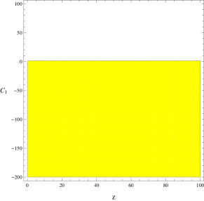
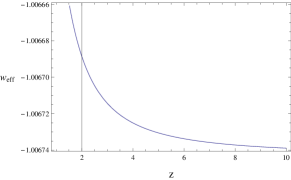
Figure 7: Left region plot shows validity region for WEC and NEC while Right plot indicates the evolution of effective EoS parameter versus cosmic time. Here $\rho_{0}=t_{0}=C_{2}=1,~{}C_{1}=100,~{}C_{3}=-0.1$ and $\omega_{m}=0,~{}l=\frac{8\pi}{3}$. For right plot, we consider $C_{2}=10$ and $q=-0.64$.

Figure 7 provides the graphical interpretation of these constraints as well as the dynamics of effective EoS parameter for this model. Clearly the left penal indicates that these constraints are valid with increasing redshift parameter where $C_{1}<0$. The right penal shows the negative values of this parameter, i.e., $\omega_{eff}<-1$, thus leading to the phantom stage of cosmic evolution.

The reconstructed phantom cosmological model is given by

$$F(B) = -\frac{(m-3)B\log(B)(3h_{0}^{2}-8\pi b_{1})}{3h_{0}^{2}(m-3)^{2}}-\frac{16b_{1}m\pi-3h_{0}^{2}(C_{2}m^{2}-6C_{2}m+9C_{2}+4m)B}{3h_{0}^{2}(m-3)^{2}}$$

$$+ \frac{16\sqrt{0.67}8b_{2}\pi(m+1)}{45h_{0}^{5}(m+3)^{3/2}(4m-3)}B^{\frac{5}{2}}+C_{1}B^{\frac{m+3}{2m}}+16b_{0}\pi.$$ (45)

The energy constraints for this model take the following form:

$$36(h_{0}e^{mN})^{4}(1+q)+8\pi(1+\omega_{m})(b_{0}+b_{1}e^{mN}+\frac{96(m+1)}{5}b_{2}e^{5mN})-2(h_{0}^{2}e^{2mN})(1+q)(-1$$

$$+3\{-\frac{(m-3)(3h_{0}^{2}-8b_{1}\pi)}{3h_{0}^{2}(m-3)^{2}}(\log(B)+\frac{1}{\ln(10)})-\frac{16b_{1}m\pi-3h_{0}^{2}(C_{2}m^{2}-6C_{2}m+9C_{2}+4m)}{3h_{0}^{2}(m-3)^{2}}$$

$$+\frac{16\sqrt{0.67}8b_{2}\pi(m+1)}{45h_{0}^{5}(m+3)^{3/2}(4m-3)}(\frac{5}{2})B^{\frac{3}{2}}+C_{1}(\frac{m+3}{2m})B^{\frac{m+3}{2m}-1}\})-18(h_{0}e^{mN})^{4}(-4+j-3q)$$

$$\times(-\frac{(m-3)(3h_{0}^{2}-8b_{1}\pi)}{3h_{0}^{2}(m-3)^{2}}(\frac{1}{B\ln(10)})+\frac{4\sqrt{0.67}8b_{2}\pi(m+1)}{3h_{0}^{5}(m+3)^{3/2}(4m-3)}B^{\frac{1}{2}}+C_{1}(\frac{m+3}{2m})(\frac{m+3}{2m}-1)B^{\frac{m+3}{2m}-2})$$

$$+36(h_{0}e^{2mN})^{4}(-4+j-3q)^{2}(-\frac{(m-3)(3h_{0}^{2}-8b_{1}\pi)}{3h_{0}^{2}(m-3)^{2}}(\frac{1}{B\ln(10)})+\frac{\sqrt{\frac{48}{27}}8b_{2}\pi(m+1)}{h_{0}^{5}(m+3)^{3/2}(4m-3)}\frac{1}{2}B^{\frac{-1}{2}}$$

$$+C_{1}(\frac{9-m^{2}}{4m^{2}})(\frac{3(1-m)}{2m})B^{\frac{3-5m}{2m}})\geq 0,$$ (46)

$$\frac{1}{2}(6h_{0}^{2}e^{2mN}-(-\frac{(m-3)B\log(B)(3h_{0}^{2}-8\pi b_{1})}{3h_{0}^{2}(m-3)^{2}}-\frac{16b_{1}m\pi-3h_{0}^{2}(C_{2}m^{2}-6C_{2}m+9C_{2}+4m)B}{3h_{0}^{2}(m-3)^{2}}$$

$$+\frac{16\sqrt{0.67}8b_{2}\pi(m+1)}{45h_{0}^{5}(m+3)^{3/2}(4m-3)}B^{\frac{5}{2}}+C_{1}B^{\frac{m+3}{2m}}+16b_{0}\pi))+8\pi(b_{0}+b_{1}e^{mN}+\frac{96(m+1)}{5}b_{2}e^{5mN})$$

$$-3(h_{0}e^{mN})^{2}(1+q)(-\frac{(m-3)(3h_{0}^{2}-8b_{1}\pi)}{3h_{0}^{2}(m-3)^{2}}(\log(B)+\frac{1}{\ln(10)})-\frac{16b_{1}m\pi-3h_{0}^{2}(C_{2}m^{2}-6C_{2}m+9C_{2}+4m)}{3h_{0}^{2}(m-3)^{2}}$$

$$+\frac{16\sqrt{0.67}8b_{2}\pi(m+1)}{45h_{0}^{5}(m+3)^{3/2}(4m-3)}(\frac{5}{2})B^{\frac{3}{2}}+C_{1}(\frac{m+3}{2m})B^{\frac{m+3}{2m}-1})-18(h_{0}e^{mN})^{4}(-4+j-3q)$$

$$\times(-\frac{(m-3)(3h_{0}^{2}-8b_{1}\pi)}{3h_{0}^{2}(m-3)^{2}}(\frac{1}{B\ln(10)})+\frac{4\sqrt{0.67}8b_{2}\pi(m+1)}{3h_{0}^{5}(m+3)^{3/2}(4m-3)}B^{\frac{1}{2}}+C_{1}(\frac{m+3}{2m})(\frac{m+3}{2m}-1)B^{\frac{m+3}{2m}-2})\geq 0.$$

(47)

Further, the corresponding effective EoS parameter can be written as

$$\omega_{eff} = [\omega_{m}(b_{0}+b_{1}e^{mN}+\frac{96(m+1)}{5}b_{2}e^{5mN})+\frac{1}{8\pi}\{\frac{1}{2}(-6h_{0}^{2}e^{2mN}-\frac{(m-3)B\log(B)(3h_{0}^{2}-8\pi b_{1})}{3h_{0}^{2}(m-3)^{2}}$$

$$- \frac{16b_{1}m\pi-3h_{0}^{2}(C_{2}m^{2}-6C_{2}m+9C_{2}+4m)B}{3h_{0}^{2}(m-3)^{2}}+\frac{16\sqrt{0.67}8b_{2}\pi(m+1)}{45h_{0}^{5}(m+3)^{3/2}(4m-3)}B^{\frac{5}{2}}+C_{1}B^{\frac{m+3}{2m}}+16b_{0}\pi)$$

$$- mh_{0}^{2}e^{2mN}(2+3(-\frac{(m-3)(3h_{0}^{2}-8b_{1}\pi)}{3h_{0}^{2}(m-3)^{2}}(\log(B)+\frac{1}{\ln(10)})-\frac{16b_{1}m\pi-3h_{0}^{2}(C_{2}m^{2}-6C_{2}m+9C_{2}+4m)}{3h_{0}^{2}(m-3)^{2}}$$ (48)

$$+ \frac{16\sqrt{0.67}8b_{2}\pi(m+1)}{45h_{0}^{5}(m+3)^{3/2}(4m-3)}(\frac{5}{2})B^{\frac{3}{2}}+C_{1}(\frac{m+3}{2m})B^{\frac{m+3}{2m}-1}))-9h_{0}^{2}e^{2mN}(-\frac{(m-3)(3h_{0}^{2}-8b_{1}\pi)}{3h_{0}^{2}(m-3)^{2}}$$

$$\times (\log(B)+\frac{1}{\ln(10)})-\frac{16b_{1}m\pi-3h_{0}^{2}(C_{2}m^{2}-6C_{2}m+9C_{2}+4m)}{3h_{0}^{2}(m-3)^{2}}+\frac{16\sqrt{0.67}8b_{2}\pi(m+1)}{45h_{0}^{5}(m+3)^{3/2}(4m-3)}(\frac{5}{2})B^{\frac{3}{2}}$$

$$+ C_{1}(\frac{m+3}{2m})B^{\frac{m+3}{2m}-1})+12m(m+3)h_{0}^{3}e^{3mN}((12h_{0}^{2}m(m+3)e^{2mN})(-\frac{(m-3)(3h_{0}^{2}-8b_{1}\pi)}{3h_{0}^{2}(m-3)^{2}}(\frac{1}{B\ln(10)})$$

$$+ \frac{\sqrt{\frac{48}{27}}8b_{2}\pi(m+1)}{h_{0}^{5}(m+3)^{3/2}(4m-3)}\frac{1}{2}B^{\frac{-1}{2}}+C_{1}(\frac{9-m^{2}}{4m^{2}})(\frac{3(1-m)}{2m})B^{\frac{3-5m}{2m}})+2m(-\frac{(m-3)(3h_{0}^{2}-8b_{1}\pi)}{3h_{0}^{2}(m-3)^{2}}(\frac{1}{B\ln(10)})$$

$$+ \frac{4\sqrt{0.67}8b_{2}\pi(m+1)}{3h_{0}^{5}(m+3)^{3/2}(4m-3)}B^{\frac{1}{2}}+C_{1}(\frac{m+3}{2m})(\frac{m+3}{2m}-1)B^{\frac{m+3}{2m}-2}))\}][b_{0}+b_{1}e^{mN}+\frac{96(m+1)}{5}b_{2}e^{5mN}$$

$$+ \frac{1}{8\pi}\{-3h_{0}e^{mN}(12h_{0}^{3}m(m+3)e^{3mN}(-\frac{(m-3)(3h_{0}^{2}-8b_{1}\pi)}{3h_{0}^{2}(m-3)^{2}}(\frac{1}{B\ln(10)})+\frac{4\sqrt{0.67}8b_{2}\pi(m+1)}{3h_{0}^{5}(m+3)^{3/2}(4m-3)}B^{\frac{1}{2}}$$

$$+ C_{1}(\frac{m+3}{2m})(\frac{m+3}{2m}-1)B^{\frac{m+3}{2m}-2}))+(3mh_{0}^{2}e^{2mN}+9h_{0}^{2}e^{2mN})(-\frac{(m-3)(3h_{0}^{2}-8b_{1}\pi)}{3h_{0}^{2}(m-3)^{2}}(\log(B)+\frac{1}{\ln(10)})$$

$$- \frac{16b_{1}m\pi-3h_{0}^{2}(C_{2}m^{2}-6C_{2}m+9C_{2}+4m)}{3h_{0}^{2}(m-3)^{2}}+\frac{16\sqrt{0.67}8b_{2}\pi(m+1)}{45h_{0}^{5}(m+3)^{3/2}(4m-3)}(\frac{5}{2})B^{\frac{3}{2}}+C_{1}(\frac{m+3}{2m})B^{\frac{m+3}{2m}-1})$$

$$- \frac{1}{2}(-6h_{0}^{2}e^{2mN}-\frac{(m-3)B\log(B)(3h_{0}^{2}-8\pi b_{1})}{3h_{0}^{2}(m-3)^{2}}-\frac{16b_{1}m\pi-3h_{0}^{2}(C_{2}m^{2}-6C_{2}m+9C_{2}+4m)B}{3h_{0}^{2}(m-3)^{2}}$$

$$+ \frac{16\sqrt{0.67}8b_{2}\pi(m+1)}{45h_{0}^{5}(m+3)^{3/2}(4m-3)}B^{\frac{5}{2}}+C_{1}B^{\frac{m+3}{2m}}+16b_{0}\pi)\}]^{-1}.$$

The graphical illustration of energy constraints behavior and effective EoS parameter is presented in Figure 8.

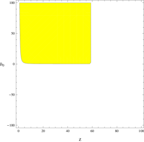
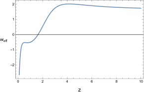
Figure 8: Left region plot shows validity region for WEC and NEC while Right plot indicates the evolution of effective EoS parameter versus cosmic time. For left plot, we take $b_{1}=2,~{}b_{2}=-0.1,~{}C_{2}=C_{1}=C_{3}=1,~{}m=2,~{}h_{0}=0.7,~{}q=-1,~{}j=1.02$ and $\omega_{m}=0$.

It is clear form the graph that the WEC and NEC are consistent for small values of redshift function, i.e., $z\leq 60$ with only positive values of $b_{0}$. The effective EoS parameters graph shows that……

VI Conclusion

Recently, teleparallel theory of gravity and its modifications have attained significant attention of the researchers for discussing various issues in cosmology. In the present paper, we have discussed the energy constraints validity and the effective EoS parameter evolution in a modified teleparallel gravity namely $f(T,B)$ theory. Actually, the $f(T,B)$ theory is formulated with the aim to unify both $f(R)$ and $f(T)$ gravitational frameworks and thus to see how these theories are connected with each other 27 . It is found that under some specified limits, this theory reduces to $f(T)$ and $f(R)$ theories. For discussing the possible constraints on the free parameters, we have used some famous cosmological models obtained by the reconstruction scheme in a recent paper 28 . Firstly, we have derived the general energy conditions directly from the effective energy-momentum tensor under the transformation $\rho\rightarrow\rho_{eff}$ and $p_{eff}\rightarrow{p}_{eff}$. Then we explore the particular forms of these constraints using the reconstructed $f(T,B)$ function for four different cosmological models namely: De Sitter universe, power law cosmology, $\Lambda$CDM universe and Phantom universe model. It is seen that in every case, there are many free variables that need to be fixed. We have chosen some specific values for some of these free parameters while others are restricted graphically in order to make sure the consistency of these energy bounds. Furthermore, we have used another particular form of the function given by $f(T,B)=-T+F(B)$ and discussed the validity of WEC and NEC in terms of graphical regions by fixing the free parameters in all four cases. The obtained results can be summarized in the form of the following table:

Table 1: The ranges of free parameters for the validity of WEC and NEC obtained through graphs.

Model	Free Parameters Choice	Obtained Ranges of free parameters for Validity
$DeSitterUniverseCaseI$	$K=1,~{}\omega_{m}=0,~{}\rho_{0}=1$	$-20\leq f_{0}\leq 200,~{}90\leq\tilde{f_{0}}\leq 170$
$CaseII$	$H_{0}=0.718,~{}\rho_{0}=0.001,~{}\omega_{m}=0$	$C_{1}<0,~{}-1\leq q\leq 2$
$PowerlawModelCaseI$	$\omega_{m}=0,~{}t_{0}=\rho_{0}=C_{2}=C_{3}=1,$	$0\leq C_{1}\leq 200,~{}0\leq t\leq 40$
	$h=10$
$CaseII$	$\rho_{0}=t_{0}=C_{2}=C_{3}=1,$	Small $t$ values with $-100\leq C_{1}\leq 100$
	$\omega_{m}=0,~{}h=10$	Also, $C_{1}\leq 0$ and $30\leq t\leq 50$
$\Lambda CDMCaseI$	$l=\frac{8\pi}{3},~{}C_{2}=10,~{}\omega_{m}=0,~{}a_{0}=1=\rho_{0},$	$C_{1}>0$ and $z>0$
	$C_{2}=C_{3}=10$
$CaseII$	$\rho_{0}=t_{0}=C_{2}=1,~{}C_{3}=-0.1,$	$z>0,~{}C_{1}<0$
	$\omega_{m}=0,~{}l=\frac{8\pi}{3},~{}C_{2}=10,~{}q=-0.64$
$PhantomModelCaseI$	$h=0.1,~{}\omega_{m}=0,~{}m=1,~{}j=1.02,~{}q=-1,$	$b_{0}>0,~{}z\geq 3$
	$b_{1}=b_{2}=-50,~{}C_{1}=C_{2}=C_{3}=1$
$CaseII$	$b_{1}=b_{2}=-50,~{}C_{2}=10,~{}C_{1}=C_{3}=1,$	$z\leq 60,~{}b_{0}>0$
	$m=1,~{}h_{0}=0.1,~{}q=-1,~{}j=1.02,~{}\omega_{m}=0$

Further we have discussed the evolution of effective EoS parameter versus cosmic time $t$ or redshift function $z$ by fixing the free parameters in all four cases graphically. The choices of the free parameters used here are exactly same as either we used in validity region graphs of WEC and NEC or obtained through the graphs. The obtained ranges of EoS parameter are then compared with the observational ranges as discussed in literature and summarized in the form of the table 2. It is seen that in all cases, the universe model either corresponds to quintessence era or phantom cosmic era of universe evolution and $\Lambda$CDM phase. Our results are consistent with WMAP9 observational data hinshaw ; $1.073^{+0.090}_{-0.089}$ (WMAP+eCMB+BAO+H₀), $1.084\pm 0.0063$ (WMAP+eCMB+BAO+H₀) and latest Planck results ade $\omega=1.09\pm 0.17$ (95% Planck+WP+Union 2.1).

Table 2: Comparison of obtained ranges of effective EoS parameter with the observed ranges given in literature.

Model	Free Parameters Choice	Effective EoS Range
$DeSitterUniverseCaseI$	$K=1,~{}\omega_{m}=0,~{}\rho_{0}=1,~{}\tilde{f}_{0}=-2$	$-1.06\leq\omega_{eff}\leq-1$
$CaseII$	$H_{0}=0.718,~{}\rho_{0}=0.001,~{}\omega_{m}=0$	$-1.0163\leq\omega_{eff}\leq-1.0159$
$PowerlawModelCaseI$	$\omega_{m}=0,~{}t_{0}=\rho_{0}=C_{2}=C_{3}=1,$	$-0.968\leq\omega_{eff}\leq-0.962$
	$h=10,~{}C_{1}=100$
$CaseII$	$\rho_{0}=t_{0}=C_{2}=C_{3}=1,$	$-1.05\leq\omega_{eff}\leq-1.25$
	$\omega_{m}=0,~{}h=10,~{}C_{1}=10$
$\Lambda CDMCaseI$	$l=\frac{8\pi}{3},~{}C_{2}=10,~{}\omega_{m}=0,~{}a_{0}=1=\rho_{0},$	$-0.998622\leq\omega_{eff}\leq-0.998610$
	$C_{1}=1000,~{}C_{2}=C_{3}=10$
$CaseII$	$\rho_{0}=t_{0}=C_{2}=1,~{}C_{1}=100,~{}C_{3}=-0.1,$	$-1.00674\leq\omega_{eff}\leq-1.00666$
	$\omega_{m}=0,~{}l=\frac{8\pi}{3},~{}C_{2}=10,~{}q=-0.64$
$PhantomModelCaseI$	$h_{0}=-0.1,~{}\omega_{m}=0,~{}m=2,~{}j=1.02,~{}q=-1$	$\omega_{eff}<-1$
	$b_{0}=1,~{}b_{1}=2,~{}b_{2}=0.0001,~{}C_{1}=C_{2}=C_{3}=1$
$CaseII$	$h_{0}=0.7,~{}\omega_{m}=0,~{}m=2,~{}j=1.02,~{}q=-1$	$\omega_{eff}<-1$
	$b_{0}=1,~{}b_{1}=2,~{}b_{2}=-0.1,~{}C_{1}=C_{2}=C_{3}=1$

It would be interesting to investigate the possible constraints on the free parameters using matter density perturbations for some other well-known models of cosmology in $f(T,B)$ gravity.

References

- (1) Weyl, H.: Gravitation und Elektrizitat. Sitzungsber. Preuss. Akad. Wissensch. 1918(1918)465.
- (2) Raifeartaigh, L. O.: The Dawning of Gauge Theory, Princeton University Press, Princeton (1998).
- (3) Raifeartaigh, L. O. and Straumann, N.: Rev. Mod. Phys. 72(2000)1.
- (4) Einstein, A.: Auf die Riemann-Metrik und den Fern-Parallelismus gegründete einheitliche Feldtheorie. Math. Ann. 102(1930)685. For an English translation, together with three previous essays, see A. Unzicker, T. Case, Unified field theory based on Riemannian metrics and distant parallelism. physics/0503046.
- (5) Kaluza, T.: Sitzungsber. Preuss. Akad. Wiss. Berlin (Math. Phys) 1921(1921)966.
- (6) Klein, O. Z.: Phys. 37(1926)895.
- (7) Cartan, E.: Ann. Sci. c. Norm. Super. 40(1923)325.
- (8) Cartan, E.: Ann. Sci. c. Norm. Super. 41(1924)1.
- (9) Mller, C.: K. Dan. Vidensk. Selsk. Mat. Fys. Skr. 1(1961)10.
- (10) Mller, C.: K. Dan. Vidensk. Selsk. Mat. Fys. Skr. 89(1978)13.
- (11) Pellegrini, C and Plebanski, J.: K. Dan. Vidensk. Selsk. Mat. Fys. Skr. 2(1962)2.
- (12) Cho, Y.M.: Phys. Rev. D 14(1976)2521.
- (13) Hayashi, K. and Shirafuji, T.: Phys. Rev. D 19(1979)3524.
- (14) Hayashi, K. and Nakano, T.: Prog. Theor. Phys. 38(1967)491.
- (15) Hayashi, K.: Nuovo Cimento A 16(1973)639.
- (16) Hayashi, K.: Phys. Lett. B 69(1977)441.
- (17) Aldrovandi, R. and Pereira, J.G.: Teleparallel Gravity: An Introduction. Fundamental Theories of Physics, Springer Dodrecht, Heidelberg 173 (2013).
- (18) Maluf, J.W.: Ann. Phys. 525(2013)339 (arXiv:1303.3897).
- (19) Ferraro, R. and Fiorini, F.: Phys. Rev. D 75(2007)084031; Bengochea, G.R. and Ferraro, R.: Phys. Rev. D 79(2009)124019; Linder, E.V.: Phys. Rev. D 81(2010)127301; Wang, T.: Phys. Rev. D 84(2011)024042; Dent, J.B., Dutta, S. and Saridakis, E.N.: J. Cosmol. Astropart. Phys. 01(2011)009; Bohmer, C.G., Harko, T. and Lobo, F.S.N.: Phys. Rev. D 85(2012)044033; Wu, Y.P. and Geng, C.Q.: J. High Energy Phys. 11(2012)142; Aviles, A., Bravetti, A., Capozziello, S. and Luongo, O.: Phys. Rev. D 87(2013)064025; Paliathanasis, S. et al.: Phys. Rev. D 89(2014)104042; Wheeler, J.T.: Nucl. Phys. B 268(1986)737; Nojiri, I.S., Odintsov, S.D. and Sasaki, M.: Phys. Rev. D 71(2005)123509; De Felice, A. and Tsujikawa, S.: Phys. Rev. D 80(2009)063516; M. Zubair, Int. J. Mod. Phys. D 25, no. 05, 1650057 (2016); M. Zubair and G. Abbas, Astrophys. Space Sci. 361, no. 1, 27 (2016); M. Zubair, Adv. High Energy Phys. 2015, 292767 (2015).
- (20) Chandia, O. and Zanelli, J.: Phys. Rev. D 55(1997)7580; Harko, T., Lobo, F.S.N., Otalora, G. and Saridakis, E.N..: Phys. Rev. D 89(2014)124036; Kofinas, G. and Saridakis, E.N.: Phys. Rev. D 90(2014)084044; Kofinas, G., Leon, G. and Saridakis, E.N.: Class. Quant. Grav. 31(2014)175011; Bahamonde, S. and Bohmer, C.G.: Eur. Phys. J. C 76(2016)578.
- (21) Zubair, M. and Waheed, S.: Astrophys. Space Sci. 355(2015)361; Zubair, M. and Waheed, S. Astrophys. Space Sci. 360, no. 2, 68 (2015).
- (22) S. Nojiri and S. D. Odintsov, eConf C 0602061 (2006) 06 [Int. J. Geom. Meth. Mod. Phys. 4, 115 (2007)].
- (23) S. Nojiri and S. D. Odintsov, Phys. Rept. 505, 59 (2011).
- (24) S. Capozziello and V. Faraoni, Beyond Einstein Gravity (Springer, Dordrecht, 2010).
- (25) S. Capozziello and M. De Laurentis, Phys. Rept. 509, 167 (2011).
- (26) K. Bamba, S. Capozziello, S. Nojiri and S. D. Odintsov, Astrophys. Space Sci. 342, 155 (2012).
- (27) A. Joyce, B. Jain, J. Khoury and M. Trodden, Phys. Rept. 568, 1 (2015).
- (28) K. Koyama, Rept. Prog. Phys. 79, 046902 (2016).
- (29) K. Bamba and S. D. Odintsov, Symmetry 7, 220 (2015).
- (30) Y. F. Cai, S. Capozziello, M. De Laurentis and E. N. Saridakis, Rept. Prog. Phys. 79, 106901 (2016).
- (31) S. Nojiri, S. D. Odintsov and V. K. Oikonomou, Phys. Rept. 692, 1 (2017).
- (32) K. Bamba, S. Nojiri and S. D. Odintsov, JCAP 0810, 045 (2008).
- (33) K. Bamba, C. Q. Geng, S. Nojiri and S. D. Odintsov, Phys. Rev. D 79, 083014 (2009).
- (34) K. Bamba, S. D. Odintsov, L. Sebastiani and S. Zerbini, Eur. Phys. J. C 67, 295 (2010).
- (35) K. Bamba, R. Myrzakulov, S. Nojiri and S. D. Odintsov, Phys. Rev. D 85, 104036 (2012).
- (36) Sotiriou, T.P. and Faraoni, V.: Rev. Mod. Phys. 82(2010)451 (arXiv:0805.1726).
- (37) Felice, A.D. and Tsujikawa, S.: Liv. Rev. Rel. 13(2010)3 (arXiv:1002.4928).
- (38) Ferraro, R. and Fiorini, F.: Phys. Rev. D 75(2007)084031 (arXiv:gr-qc/0610067).
- (39) Li, B., Sotiriou, T.P. and Barrow, J.D.: Phys. Rev. D 83(2011)064035 (arXiv:1010.1041).
- (40) Sotiriou, T.P., Li, B. and Barrow, J.D.: Phys. Rev. D 83(2011)104030 (arXiv:1012.4039).
- (41) Bahamonde, S., Bohmer, C.G. and Wright, M.: Phys. Rev. D 92(2015)104042 (arXiv:1508.05120).
- (42) Bahamonde, S., Zubair, M. and Abbas, G.: Phys. of Dark Universe 19(2018)78.
- (43) Santos, J. et al.: Phys. Rev. D 76(2007)083513; Santos, J, Reboucas, M.J. and Alcaniz, J.S.: Int. J. Mod. Phys. D 19(2010)1315; Liu, Di and Reboucas, M.J.: Phys. Rev. D 86(2012)083515; Garcia, N.M.: Phys. Rev. D 83(2011)104032; Zhao, Y.Y.: Eur. Phys. J. C 72(2012)1924; Bertolami, O. and Sequeira, M.C.: Phys. Rev. D 79(2009)104010; Wang, J. et al.: Phys. Lett. B 689(2010)133; Wang, J. and Liao, K.: Class. Quantum Grav. 29(2012)215016; Atazadeh, K., Khaleghi, A., Sepangi, H.R. and Tavakoli, Y.: Int. J. Mod. Phys. D 18(2009)1101.
- (44) Sharif, M. and Waheed, S.: Advances in High Energy Phys. 2013(2013)253985.
- (45) Sharif, M. and Zubair, M.: J. Phys. Soc. Jpn. 82(2013)014002.
- (46) Sharif, M. and Zubair, M.: J. High. Energy Phys. 12(2013)079.
- (47) Waheed, S. and Zubair, M.: Astrophys. Space Sci 359(2016)47.
- (48) Capozziello, S., Cardone, V.F., Farajollahi, H. and Ravanpak, A.: Phys. Rev. D 84(2011)043527.
- (49) Hinshw, G. et al., Astrophys. J. Suppl. Ser. 208, 19 (2013).
- (50) Ade, P.A.R., et al., Astronomy and Astrophysics. 571, A1 (2014); Spergel, D. N., et al., Astrophys. J. Suppl. Ser. 170, 37 (2007)