Sequence to Logic with Copy and Cache

Abstract

Generating logical form equivalents of human language is a fresh way to employ neural architectures where long short-term memory effectively captures dependencies in both encoder and decoder units. The logical form of the sequence usually preserves information from the natural language side in the form of similar tokens, and recently a copying mechanism has been proposed which increases the probability of outputting tokens from the source input through decoding. In this paper we propose a caching mechanism as a more general form of the copying mechanism which also weighs all the words from the source vocabulary according to their relation to the current decoding context. Our results confirm that the proposed method achieves improvements in sequence/token-level accuracy on sequence to logical form tasks. Further experiments on cross-domain adversarial attacks show substantial improvements when using the most influential examples of other domains for training.

1 Introduction

Understanding human language has a long history, and interpreting language for machine execution is a key component of artificial intelligence and machine learning Dong and Lapata (2016); Jia and Liang (2016). Multiple techniques have been proposed in a neural setting for text to text translation Bahdanau et al. (2014); Sutskever et al. (2014); Luong et al. (2015) or in machine format Jia and Liang (2016); Zhong et al. (2017); Quirk et al. (2015) including, but not limited to, semantic parsing Jia and Liang (2016), code generation Quirk et al. (2015), and query generation for database systems Xu et al. (2017); Zhong et al. (2017).

Recently Jia and Liang (2016) proposed an augmented pointer network for converting a sequence to its logical form where a greedy decoder generates the next token according to the last hidden state of the source encoder augmented by a pointer to each of the source tokens. This is a very straightforward mechanism to pay attention to the source sequence which increases the chance of generating shared tokens between the natural language input and its logical form output. In this paper we introduce a “cache” to take the entire source vocabulary into account during decoding. The following example is from the GeoQuery data set Tang and Mooney (2001); Zettlemoyer and Collins (2012):

• x: what rivers flow through colorado ?

• y: answer ( A , ( river ( A ) , traverse ( A , B ) , const ( B , stateid ( colorado ) ) ) )

The previously proposed augmented pointer network increases the probability of colorado in the output logical form sequence as this entity appears in the input sentence. However, our proposed joint cache distribution aims to find semantically related tokens throughout the entire source vocabulary which hold importance in outputting relevant tokens.

For this example, the caching probability for the words ‘flow through’ turns on in this context and generates ‘traverse’ from the probability distribution over the source vocabulary. We note that the previous model proposed by Jia and Liang (2016) is expected to do the same through a general decoder trained over the data set. Our findings reveal that in some situations neither the local copy nor the general decoder are able to find in-domain vocabulary words (e.g., date for the calendar domain or author for the publications domain). Our proposed method on the other hand is able to capture these situations in different domains. While this method provides varied tokens and improves the token-level accuracy, similar to the baselines, it is not able to boost the sequence level accuracy significantly and provides marginal improvements in this metric.

In the second part we use cross-domain adversarial attack to augment our model with cached tokens in other domains. To do this we follow the influence functions used in Koh and Liang (2017) to find the most sensitive examples. Our results support the usefulness of these examples compared to the original version of training data.

2 Related Work

2.1 Sequence to logic

Semantic parsing maps natural language sentences to formal meaning representations. Semantic parsing techniques can be performed on various natural languages as well as task-specific representations of meaning. A semantic parser can be learned in a supervised or semi-supervised manner in which the natural language sentence is paired with either a logical form or its executed denotation.

Supervised Semantic Parsing In recent work on supervised semantic parsing, a natural language statement is paired with its corresponding logical meaning representation Zettlemoyer and Collins (2005); Wong and Mooney (2006); Kwiatkowski et al. (2010). The logical forms may be database queries, dependency graphs, lambda-calculus terms, among others.

Semi-Supervised Semantic Parsing Due to the lack of large supervised datasets, semi-supervised semantic parsing is often performed on denotations from question-answer pairs, which are much cheaper to obtain than corresponding logical forms. Liang et al. (2013) map questions to answers using latent logical forms. Cheng et al. (2017) use a transition-based approach to convert natural language sentences to intermediate predicate-argument representation structures then grounded to a knowledge base. Kwiatkowski et al. (2013) build a logical-form meaning representation which is fed to an ontology matching model. For this paper, however, we focus on neural supervised approaches to semantic parsing.

3 Sequence to Logic with Copy and Cache

Let $y^{t}=\textrm{argmax}(\dot{\beta})$ be the next token to be generated at time stamp $t$ in a standard sequence to sequence decoding process. We refer the reader to Jia and Liang (2016) for the equations upon which we base ours below. As in Jia and Liang (2016) we create a distribution over the target vocabulary as well as a copying distribution. However, our copying mechanism constitutes both a distribution over the source sentence and the entire source vocabulary combined with the target distribution through the concatenation in Equation 1:

$$e_{ji}=[s_{j}^{T}W^{(a)}b_{i}]+[z_{t}\odot f(s_{j},c_{j})]$$ (1)

$$\alpha_{ji}=\frac{\exp(e_{ji})}{\sum_{i^{\prime}=1}^{m}\exp(e_{ji^{\prime}})}$$ (2)

$$c_{j}=\sum_{i=1}^{|V_{s}|}\alpha_{ji}b_{i}$$ (3)

$$P(y_{j}=w|x,y_{1:j-1})\propto\exp(U_{w}[s_{j},c_{j}])$$ (4)

$$P(y_{j}=\textrm{copy}[i]|x,y_{1:j-1})\propto\exp(e_{ji})$$ (5)

where $e_{ji}$ is the normalized attention score of state $s_{j}$ to the source annotation $b_{i}$; $w$ is the target candidate token and copy[$i$] is the candidate token to be copied from the source sequence. We refer to $f(s_{j},c_{j})$ in this equation as the cache function, as it aims to keep track of the history with which words in the input vocabulary and input sequence appear in contexts relevant to the target output. One simple approximation for $f(s_{j},c_{j})$ is $f(s_{j},c_{j})=s_{j}^{T}W^{(a)}W^{(h)}$ where $W^{(a)}\in\mathbb{R}^{d\times 4d}$ and $W^{(h)}\in\mathbb{R}^{4d\times|V_{s}|}$ is the cache matrix (see the supplementary material for more examples of this function). It’s worth noting that since we select the bi-directional LSTM for our encoding annotations, $W^{(a)}\in\mathbb{R}^{d\times(\overrightarrow{2d}+\overleftarrow{2d})}$, where $d$ is the hidden layer size and $2d$ results from the combination of the $h$ and $c$ parameters of the LSTM model. $z_{t}=\sigma{([s^{T}_{j}U_{z_{t}}]+[c^{T}_{j}W_{z_{t}}])}$ is a reset gate for the context $c_{j}$ and state $s_{j}$ where $U_{z_{t}},W_{z_{t}}\in\mathbb{R}^{d\times|V_{s}|}$. This is inspired by the forget and reset gates in LSTM’s and Gated Recurrent Units. As the history matrix calculates often a large distribution, this distribution may be noisy. This reset gate allows us to diminish the effect of irrelevant words, and we expect that $W^{(h)}$ will be learned over the source vocabulary.

Figure 1: A caching gate for decoding. For prediction we use both the local attention $W^{(a)}$ and the caching matrix $W^{(h)}$.

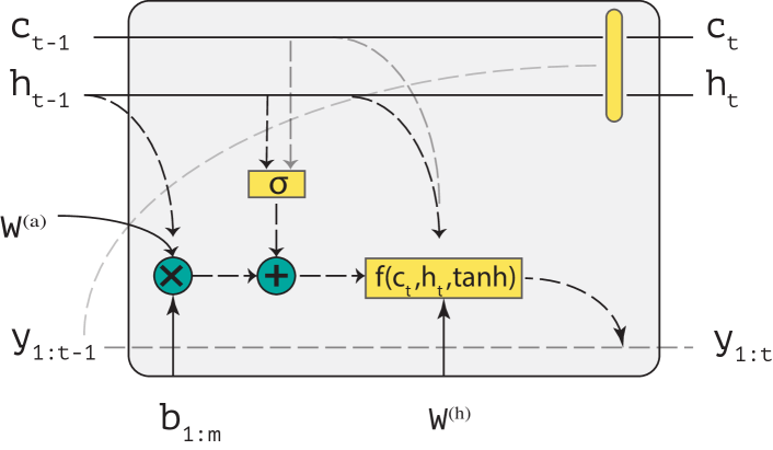
Fig. 1 shows the sketch of the proposed caching mechanism. The remaining equations amount to a standard attention mechanism with our additional caching mechanism analogous to the copying equations in Jia and Liang (2016).

Influence functions Recently Koh and Liang (2017) introduced influence functions for a number of classification tasks to find the most influential examples for testing. The central goal of these functions is the non-parametric estimation of $\hat{\theta}_{\epsilon,\textbf{z}}=\arg\min_{\theta}\sum_{z_{i}\notin\textbf{z}}\frac{1}{n}\mathcal{L}(z_{i},\theta)+\epsilon\mathcal{L}(\textbf{z},\theta,t_{k})$ (i.e., parameters to learn) by up-weighting $\forall z_{i}\in\textbf{z}$ (i.e., batch of examples $z_{j}=(x_{j},y_{j})$) or $\hat{\theta}_{\epsilon,z_{j}}=\arg\min_{\theta}\sum_{z_{i}\neq z_{j}}\frac{1}{n}\mathcal{L}(z_{i},\theta)+\epsilon\mathcal{L}(z_{j},\theta,t_{k})$ by up-weighting one particular example $z_{j}$ Wasserman (2006); Cook and Weisberg (1980). Later in Section 4.2 we study the impacts of other domains in caching useful words both on domain-level (i.e., $\hat{\theta}_{\epsilon,\textbf{z}}$) and example level (i.e., $\hat{\theta}_{\epsilon,z_{j}}$) by adversarial attacks on binary classification loss $\mathcal{L}(.)$. Our experiments in Section 4.3 show that a close domain z can provide useful information for predicting $y_{i}$.

4 Experiments

4.1 Experimental Settings

Data sets: We evaluate the models based on standard semantic parsing datasets.

GeoQuery: The GEO dataset Wong and Mooney (2006) contains natural language queries about U.S. geography and their associated Prolog queries. We use the standard split of 680 training examples and 200 test examples Zettlemoyer and Collins (2005). We follow the preprocessing of Jia and Liang (2016) and use De Bruijn index notation for variable-name standardization.

Overnight: The Overnight dataset contains natural language paraphrases paired with logical forms from eight domains such as restaurants, publications and basketball. The dataset was developed by Wang and Yang (2015) using a crowdsourcing experiment in which Amazon Mechanical Turkers created paraphrases for given logical forms which were generated from a grammar.

Parameter settings: We set the hidden size $|h_{t}|=200$ and the input embedding dimension $|x_{t}|=100$. We also use Long Short-Term Memory (LSTM) units as the basic encoder/decoder unit in all of our experiments. We initialize all the variables with a uniform distribution in $[-1,1]$ and use stochastic gradient descent as our learning method with a $0.5$ learning rate decreasing by half at each epoch. We set the number of epochs to $30$ for all the experiments.

In the decoding process we assume a maximum length of $100$ for all the data sets and stop decoding after predicting the end of the sentence indicator.

4.2 Results and Discussion

In this part we assess the validity of the proposed network on two different tasks. To be fair, we fix the settings for all the runs and then test the performance over our sampled datasets. For example, we do not use any rule-based augmented samples as in Jia and Liang (2016), which is a domain-specific technique and boosts the performance for all the baselines.

ID	GEOQUERY		GEOQUERY-S		OVERNIGHT
	SEQ	TOK	SEQ	TOK	SEQ	TOK
copy	0.771	0.883	0.58	0.865	0.601	0.868
copy&cache	0.775	0.901	0.70	0.886	0.610	0.871

Table 1: Accuracy of different semantic parsing approaches on three collections. GEOQUERY-S is the stripped version of GEOQUERY.

(a) pub^∗+cal:seq

(b) pub^∗+cal:tok

(c) pub^∗+cal:den

Figure 2: Cross-domain adversarial attack between publications domain and calendar. Results are in sequence-level (seq) and token-level (tok), and denotation-level (den). Auperscript ^∗ indicates that we used the most influential examples of pub. We add these examples at different size steps.

Table 4 shows the experimental results on semantic parsing datasets. GEOQUERY-S, is a variation of the GEOQUERY dataset where logical form tokens are replaced by human language words. As shown in the table, the copy&cache algorithm works as well as the original version proposed by Jia and Liang (2016) but has further improvements in different collections. The highest improvement is for GEOQUERY-S where it is more likely to copy a human language token to the logic form while the source sequence may have different variants of this token. In the supplementary material, we provided a number of examples where the original coping mechanism was not able to predict the correct logic sequence (e.g., providing semantically related words or correcting the miss-spelling tokens in the source sequence). We also conducted a set of experiments on WikiSQL, the sequence to SQL dataset Zhong et al. (2017) and ATIS Zettlemoyer and Collins (2007), a flight data set, but we do not report the results since these datasets are designed for execution level comparisons in real databases and achieve comparatively lower results in sequence-level accuracy.

4.3 Cross-domain adversarial attack

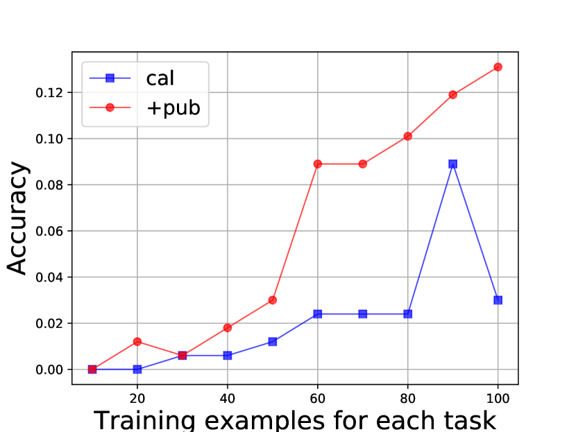
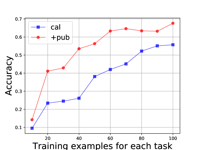
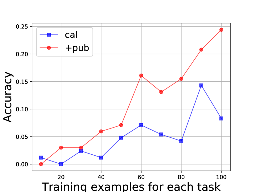
In this section we experiment with a type of transfer learning to copy the cached tokens from other domains while preserving the accuracy of the running system Su and Yan (2017); Fan et al. (2017). First we fixed calendar as a test domain from OVERNIGHT and conducted several leave-one-out experiments to find the closest domains for calendar. Our experiments have shown atis as the farthest domain from calendar in OVERNIGHT and publications as the closest one. We then repeated this experiment for each example of publications to find the most influential examples. To this aim we used cross-domain adversarial attacks based on the inflluence functions discussed in Section 3. Then the most influential examples in the binary classification task (i.e., calendar and publications) are selected to add to our sequence to logic problem. To do so, we repeated the hessian vector product (HVP) algorithm used in Koh and Liang (2017) $1000$ times and created a distribution based on the number of occurrences of each example. Then we sampled $100$ examples for our training data. Fig. 2 shows the experimental results which support the usefulness of caching from related domains. As shown in the figure the original calendar baseline over-fits to the training data (see drop in the blue line after $n=90$) while the copy&cache version generalizes better.

5 Conclusion and Future Work

In this paper we introduce a caching mechanism for encoder/decoder systems. The previous copying mechanism employed boosts performance by giving a chance for the source tokens to appear in target decoding. The proposed function extends this possibility for the entire source vocabulary that might have some semantic relationship with the current context. Experiments on sequence to logic data sets support its superiority in different evaluation metric. Our experiments on cross-domain adversarial attack show substantial improvements when we augment a test data by the closest examples from other domains. We propose this method for machine translation as a possible future work where we might copy a translation of other source tokens rather than the local one.

Appendix A Examples of cached tokens

Table 2: Examples from different domains where the decoder generated the target token from the caching distribution. As mentioned before there are three possibility to generate token: 1-general decoder 2- local copying, and 3- caching functions. These examples are in the third category.

$x$	$y$
housing units with 2 neighborhoods	( call SW.listVal. ( call SW.countComp. ( call SW.getProp. ( call SW.singleton en.housing_unit ) ( string ! type )) ( string neighborhood ) ( string = ) ( number 2 )))
article cited by article which in 2004 is published	( call SW.listValue ( call SW.filter ( call SW.getProperty ( call SW.singleton en.article ) ( string ! type ) ) ( call SW.reverse ( string cites ) ) ( string = ) ( call SW.filter ( call SW.getProperty ( call SW.singleton en.article ) ( string ! type ) ) ( string publication_date ) ( string = ) ( date 2004 -1 -1 ) ) ) )
Who won the game that took place at stadium australia, sydney (10)?	SELECT col2 FROM table_1_11236195_5 WHERE col5=’Stadium Australia , Sydney (10)’
select a block that has a width that is the same width of block 1	( call SW.listValue ( call SW.filter ( call SW.getProperty ( call SW.singleton en.block ) ( string ! type ) ) ( call SW.ensureNumericProperty ( string width ) ) ( string <= ) ( call SW.ensureNumericEntity ( call SW.getProperty en.block.block1 ( string width ) ) ) ) )

As shown in Table 2, date is a frequent word in the publications domain and many human languages contain similar tokens; in this particular example it has been generated from the cache function while there was a possibility to be generated from the target distribution or the copying distribution. Indeed here this model captures general words in this domain and adds to the logical form output when there is either no signal from either human input text (i.e., $P(y_{j}=\textrm{copy}[i]|x,y_{1:j-1})$) or the general decoder (i.e., $P(y_{j}=w|x,y_{1:j-1})$). The reason is the same for number in the housing domain and also type in blocks. The most interesting part is ,sydney where there is a typo in the source sequence in terms of tokenization. The caching functions provided the original version of this word in the logical form side.

Appendix B Examples of caching functions

Generally the caching function should work as good as the local copying version if we define robust reset functions. Table 3 shows a number of caching functions with different non-linearity ($\sigma$, tanh, or nothing) or different reset gates. Different functions hold different characteristics and sometimes work better than the proposed function in the paper. It’s worth noting that $f_{4},f_{5}$ provide minimum number of parameters to the model while keeping the token-level performance. GEOQUERY-S is a variation of the GEOQUERY dataset that we replaced logic forms like ${}_{l}oc$ with their corresponding natural language forms like $location$; we are not able to run these questions in the database though.

Table 3: Different models for the caching function.

1	$f_{1}(s_{j},c_{j})=s_{j}^{T}W^{a}W^{(h)}$
2	$f_{2}(s_{j},c_{j},\sigma)=\sigma(s_{j}^{T}W^{a}W^{(h)})$
3	$f_{3}(s_{j},c_{j},\sigma)=\sigma(s_{j}^{T}W^{a}W^{(h)}+c_{j}W^{(h)})$
4	$f_{4}(s_{j},c_{j},\sigma)=\sigma(s_{j}^{T}U_{z_{t}})$
5	$f_{5}(s_{j},c_{j},\tanh)=\tanh(s_{j}^{T}U_{z_{t}})$
6	$f_{6}(s_{j},c_{j},\sigma)=z_{t}\odot\sigma(s_{j}^{T}W^{a}W^{(h)})+{(1-z_{t})}\odot$ $\sigma(c_{j}W^{(h)})$

Table 4: Accuracy of different caching functions.

ID	GEOQUERY		GEOQUERY-S
	SEQ	TOK	SEQ	TOK
attn	0.771	0.8826	0.580	0.8648
$f_{1}(s_{j},c_{j})$	0.775	0.901	0.700	0.886
$f_{2}(s_{j},c_{j},\sigma)$	0.746	0.897	0.711	0.88
$f_{3}(s_{j},c_{j},\sigma)$	0.742	0.893	0.714	0.883
$f_{4}(s_{j},c_{j},\sigma)$	0.746	0.897	0.732	0.880
$f_{5}(s_{j},c_{j},\tanh)$	0.746	0.897	0.721	0.888
$f_{6}(s_{j},c_{j},\sigma)$	0.746	0.8968	0.732	0.883

References

- Bahdanau et al. (2014) Dzmitry Bahdanau, Kyunghyun Cho, and Yoshua Bengio. 2014. Neural machine translation by jointly learning to align and translate. CoRR abs/1409.0473. http://arxiv.org/abs/1409.0473.
- Cheng et al. (2017) Jianpeng Cheng, Siva Reddy, Vijay Saraswat, and Mirella Lapata. 2017. Learning structured natural language representations for semantic parsing. CoRR abs/1704.08387. http://arxiv.org/abs/1704.08387.
- Cook and Weisberg (1980) R Dennis Cook and Sanford Weisberg. 1980. Characterizations of an empirical influence function for detecting influential cases in regression. Technometrics 22(4):495–508.
- Dong and Lapata (2016) Li Dong and Mirella Lapata. 2016. Language to logical form with neural attention. In Proceedings of the 54th Annual Meeting of the Association for Computational Linguistics (Volume 1: Long Papers). Association for Computational Linguistics, Berlin, Germany, pages 33–43. http://www.aclweb.org/anthology/P16-1004.
- Fan et al. (2017) Xing Fan, Emilio Monti, Lambert Mathias, and Markus Dreyer. 2017. Transfer learning for neural semantic parsing. CoRR abs/1706.04326. http://arxiv.org/abs/1706.04326.
- Jia and Liang (2016) Robin Jia and Percy Liang. 2016. Data recombination for neural semantic parsing. In Association for Computational Linguistics (ACL).
- Koh and Liang (2017) Pang Wei Koh and Percy Liang. 2017. Understanding black-box predictions via influence functions. In Doina Precup and Yee Whye Teh, editors, Proceedings of the 34th International Conference on Machine Learning. International Convention Centre, Sydney, Australia, volume 70 of Proceedings of Machine Learning Research, pages 1885–1894.
- Kwiatkowski et al. (2013) Tom Kwiatkowski, Eunsol Choi, Yoav Artzi, and Luke S. Zettlemoyer. 2013. Scaling semantic parsers with on-the-fly ontology matching. In EMNLP 2013. pages 1545–1556. http://aclweb.org/anthology/D/D13/D13-1161.pdf.
- Kwiatkowski et al. (2010) Tom Kwiatkowski, Luke S. Zettlemoyer, Sharon Goldwater, and Mark Steedman. 2010. Inducing probabilistic CCG grammars from logical form with higher-order unification. In EMNLP 2010. pages 1223–1233. http://www.aclweb.org/anthology/D10-1119.
- Liang et al. (2013) Percy Liang, Michael I. Jordan, and Dan Klein. 2013. Learning dependency-based compositional semantics. Computational Linguistics 39(2):389–446.
- Luong et al. (2015) Minh-Thang Luong, Hieu Pham, and Christopher D. Manning. 2015. Effective approaches to attention-based neural machine translation. CoRR abs/1508.04025. http://arxiv.org/abs/1508.04025.
- Quirk et al. (2015) Chris Quirk, Raymond J. Mooney, and Michel Galley. 2015. Language to code: Learning semantic parsers for if-this-then-that recipes. In ACL-IJCNLP 2015. pages 878–888. http://aclweb.org/anthology/P/P15/P15-1085.pdf.
- Su and Yan (2017) Yu Su and Xifeng Yan. 2017. Cross-domain semantic parsing via paraphrasing. CoRR abs/1704.05974. http://arxiv.org/abs/1704.05974.
- Sutskever et al. (2014) Ilya Sutskever, Oriol Vinyals, and Quoc V. Le. 2014. Sequence to sequence learning with neural networks. In NIPS 2014. pages 3104–3112.
- Tang and Mooney (2001) Lappoon R Tang and Raymond J Mooney. 2001. Using multiple clause constructors in inductive logic programming for semantic parsing. In ECML. Springer, volume 1, pages 466–477.
- Wang and Yang (2015) William Yang Wang and Diyi Yang. 2015. That’s so annoying!!!: A lexical and frame-semantic embedding based data augmentation approach to automatic categorization of annoying behaviors using# petpeeve tweets. In EMNLP. pages 2557–2563.
- Wasserman (2006) Larry Wasserman. 2006. All of Nonparametric Statistics (Springer Texts in Statistics). Springer-Verlag New York, Inc., Secaucus, NJ, USA.
- Wong and Mooney (2006) Yuk Wah Wong and Raymond J. Mooney. 2006. Learning for semantic parsing with statistical machine translation. In NAACL HLT 2006. http://aclweb.org/anthology/N/N06/N06-1056.pdf.
- Xu et al. (2017) Xiaojun Xu, Chang Liu, and Dawn Song. 2017. Sqlnet: Generating structured queries from natural language without reinforcement learning. CoRR abs/1711.04436. http://arxiv.org/abs/1711.04436.
- Zettlemoyer and Collins (2005) Luke S. Zettlemoyer and Michael Collins. 2005. Learning to map sentences to logical form: Structured classification with probabilistic categorial grammars. In UAI ’05, Proceedings of the 21st Conference in Uncertainty in Artificial Intelligence, Edinburgh, Scotland, July 26-29, 2005. pages 658–666.
- Zettlemoyer and Collins (2007) Luke S. Zettlemoyer and Michael Collins. 2007. Online learning of relaxed ccg grammars for parsing to logical form. In EMNLP-CoNLL 2007. pages 678–687.
- Zettlemoyer and Collins (2012) Luke S Zettlemoyer and Michael Collins. 2012. Learning to map sentences to logical form: Structured classification with probabilistic categorial grammars. arXiv preprint arXiv:1207.1420 .
- Zhong et al. (2017) Victor Zhong, Caiming Xiong, and Richard Socher. 2017. Seq2sql: Generating structured queries from natural language using reinforcement learning. arXiv preprint arXiv:1709.00103 .