Kato-Matsumoto-type results for disentanglements

Abstract.

We consider the possible disentanglements of holomorphic map germs $f\colon(\mathbb{C}^{n},0)\to(\mathbb{C}^{N},0)$, $0<n<N$, with nonisolated locus of instability $\operatorname{Inst}(f)$. The aim is to achieve lower bounds for their (homological) connectivity in terms of $\dim\operatorname{Inst}(f)$. Our methods apply in the case of corank $1$.

MSC classification: .
Keywords: .

1. Introduction

Let $g\colon(\mathbb{C}^{n+1},0)\to(\mathbb{C},0)$ be a holomorphic function germ defining an isolated hypersurface singularity $Z=g^{-1}(\{0\})$. The Milnor fibre $M$ has the homotopy type of a wedge of $n$-dimensional real spheres, see [15]. In particular, the reduced homology of $M$ is concentrated in degree $n$. Since its appearance, this result has been subject to several generalizations and modifications. We are interested in the connections between two modifications of the original setup, which we refer to as the fibration setup and the parametrization setup.

The fibration setup generalizes the original one in two ways. In the first one, $Z$ is a higher codimension complete intersection with isolated singularity. It is a result of Hamm [7] that $M$ still has the homotopy type of a bouquet of spheres of real dimension $\dim Z$. Alternatively, one can ask $Z=g^{-1}(\{0\})$ to be a hypersurface but let the singular locus have dimension $d$. Kato and Matsumoto showed in [11] that the Milnor fibre of $g$ is at least $(n-d-1)$-connected. The fact that this holds also for non-isolated complete intersection singularities has been part of the folklore. For lack of a reference, we give a proof in Section 4.3.

In the parametrization setup, the space $Z$ is the image of a finite holomorphic map germ $f\colon(\mathbb{C}^{n},0)\to(\mathbb{C}^{N},0)$, and one would like to understand the changes in topology after perturbing $f$ to a stable map. The map germs with isolated instabilities are the $\mathcal{A}$-finite map germs, and the image of a good representative of a stabilization of $f$ is called a disentanglement. Thinking of the fibrations and parametrization settings as different instances of the general deformation theory reveals interesting connections. Milnor’s original setting, dealing with isolated hypersurface singularities, corresponds to that of $\mathcal{A}$-finite parametrization $f\colon(\mathbb{C}^{n},0)\to(\mathbb{C}^{n+1},0)$. D. Mond showed in [16] that the disentanglement has the homotopy type of a bouquet of $n$-spheres. The number of spheres in the bouquet is called the image Milnor number $\mu_{I}(f)$. Another illustrating example is Mond’s conjecture. It claims the inequality $\mu_{I}(f)\geq\mathcal{A}_{e}{\rm-codim}(f)$ – motivated, by analogy, from the trivial inequality $\mu\geq\tau$ for the Milnor and Tjurina numbers of hypersurfaces with isolated singular locus. Moving to higher codimension, the setting of Hamm’s result corresponds to that of $\mathcal{A}$-finite map germs $(\mathbb{C}^{n},0)\to(\mathbb{C}^{N},0)$ with $N>n+1$. The degrees containing the non-trivial rational homology were determined for corank one germs by Goryunov and Mond in [6]; the result being generalized to arbitrary corank by Houston in [10]. In this work, we show the analog of Kato and Matsumoto’s result for disentanglements.

The restriction we have to make is to consider only the case of corank $1$ germs with multiple point spaces of the expected dimension. In this situation the latter are complete intersections and we can study their induced deformations by means of the generalized Kato-Matsumoto Theorem. Then, we apply a spectral sequence argument due to Goryunov and Mond [6] to compute the rational homology of the disentanglement.

Just as in [6], passing through the spectral sequence looses the information about the homotopy type of the disentanglement as well as its integer homology groups.

Acknowledgements

The first author was partially supported by the ERCEA 615655 NMST Consolidator Grant and by the Basque Government through the BERC 2014-2017 program and by Spanish Ministry of Economy and Competitiveness MINECO: BCAM Severo Ochoa excellence accreditation SEV-2013-0323. The second author wishes to thank for the kind hospitality during a stay at the University of Valencia, during which the work on this subject was initiated.

2. Overview and results

We briefly outline the main theorem of this article and recall the common definitions of the objects involved. Consider a finite, holomorphic map germ

$$f\colon(\mathbb{C}^{n},0)\to(\mathbb{C}^{N},0).$$

Let $(\operatorname{Inst}(f),0)\subset(\mathbb{C}^{N},0)$ be the instability locus of $f$ (see Definition 3.1) and let $d=\dim(\operatorname{Inst}(f),0)$. We will mostly be concerned with non-isolated instability, i.e. the case $d>0$. We may choose an unfolding

$$F\colon(\mathbb{C}^{n},0)\times(\mathbb{C},0)\to(\mathbb{C}^{N},0)\times(\mathbb{C},0),\quad(x,u)\mapsto(f_{u}(x),u)$$

of $f=f_{0}$ and a good, proper representative $F\colon X\times U\to Y\times U$ thereof in a sense made precise below (cf. Definition 3.2 and Section 4.1). Using stratification theory and Thom’s isotopy lemmas one can show that the image $F(X)$ is a topological fiber bundle with fiber $f_{u}(X)$ over all $u\neq 0$ in some small disc $D\subset U$ around the origin. In case that $F$ is a $C^{0}$-stabilization (see Definition 3.1) of $f$, we call the space $Z_{u}:=f_{u}(X)$ a disentanglement of $f$. However, since our considerations also involve multiple point spaces and their induced deformations, we will have to chose the representatives accordingly. Also note that, contrary to the case of isolated instability, our notion of Milnor fiber really depends on the chosen unfolding $F$ and not only on the map germ $f$.

Theorem 2.1.

In the setup described above, the reduced homology with rational coefficients $\tilde{H}_{q}(Z_{u},\mathbb{Q})$ of a disentanglement $Z_{u}=f_{u}(X)$ of a dimensionally correct corank $1$ map germ $f\colon(\mathbb{C}^{n},0)\to(\mathbb{C}^{N},0)$ can only be nonzero in degrees $q$ with

$$q=k(n+1)-(k-1)N-s$$

for $1<k\leq\left\lfloor\frac{N}{N-n}\right\rfloor$ and $0\leq s\leq\dim\operatorname{Inst}(f)$. In the particular case $N=n+1$ one has

$$n-\dim\operatorname{Inst}(f)\leq q\leq n$$

as the range for possibly nonzero Betti numbers.

Two more points in the statement of this theorem need clarification. The first one is the notion for a map germ $f$ to be dimensionally correct. This means that the multiple point spaces of $f$ have the expected dimension, as explained in Definition 3.7. The second one is the condition on $f$ to have corank $1$. The corank of a map germ centered at the origin is defined as

(1) $$\operatorname{corank}f=n-\operatorname{rank}\operatorname{d}\!f(0),$$

where, as usual, $\operatorname{d}\!f$ denotes the differential of $f$. The dimensionally correct and corank $\leq 1$ conditions in the statement of Theorem 2.1 ensure that the multiple point spaces are complete intersections of the expected dimensions, with singularities only over the instability locus; and that the multiple point spaces of a stable perturbation are smoothings of these complete intersections. This is explained in [13], which, together with [6], forms the basis of this article. We close this section by giving some introductory examples:

Example 2.2.

The Cuspidal Edge

$$S_{\infty}\colon(x,u)\mapsto(x^{2},x^{3},u),$$

admits deformations to the germs

$$S_{k}\colon(x,u)\mapsto(x^{2},x^{3}+u^{k+1}x,u),\quad k\geq 0.$$

and to their stable perturbations, see Figure 1. For each $k$, these deformations may be obtained by taking suitable curves in the parameter space of the unfolding

$$(x,u,a,b)\mapsto(x^{2},x^{3}+x(a+bu^{k+1}),u,a,b).$$

The curve with parameter $t$ given by $t\mapsto(a,b)=(0,t)$ gives a family with generic fiber $S_{k}$ and special fiber $S_{\infty}$. Fixing $a=t^{2}$ and $b=t$ produces stable perturbations of $S_{\infty}$, with a different second Betti number for each $k$. The statement on the Betti numbers follows from the fact that the generic maps on these families are precisely the stable perturbations of $S_{k}$ (the ones obtained by fixing a small enough $b\neq 0$ and letting $a=t$). Since $S_{k}$ has $\mathcal{A}_{e}$-codimension $k$, and Mond’s conjecture holds for germs $(\mathbb{C}^{2},0)\to(\mathbb{C}^{3},0)$, the second Betti number of the image of these stable perturbations is $k$.

The germ $S_{\infty}$ also admits deformations to the “nodal edge”

$$(x,u)\mapsto(x^{2},x^{3}+tx,u),$$

which can be retracted to a simple node curve. This gives a stable perturbation of a germ of a parametrized surface singularity having non trivial homology in dimension 1.

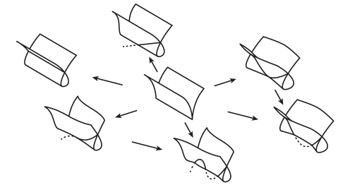
Figure 1. Unfoldings of the Cuspidal Edge

Example 2.3.

The singularity

$$B_{\infty}\colon(x,u)\mapsto(x^{2},u^{2}x,u)$$

admits deformations to the $\mathcal{A}$-finite singularities

$$B_{k}\colon(x,u)\mapsto(x^{2},u^{2}x+x^{2k+1},u),\quad k\geq 1,$$

see Figure 2. Each $B_{k}$ has codimension $k$, and thus admits a deformation to a singularity whose image has the homotopy type of a wedge of $k$ spheres of dimension two. We shall illustrate this by taking suitable curves in the parameter space of the deformation

$$(x,u)\mapsto(x^{2},u^{2}x+x(a+bx^{2}+cx^{4}),u),$$

with coordinates $(a,b,c)\in\mathbb{C}^{3}$.

The curve $t\mapsto(a,b,c)=t\cdot(1/10,-1,1)$ gives, for a small non zero parameter $t$, a stable perturbation $f_{t}$, depicted at the left top corner of Figure 1, which exhibits non-trivial homology in dimensions 1 and 2.

$t\mapsto(0,t,0)$ yields, for each $t\neq 0$, a singularity of type $B_{1}$. The curve $t\mapsto(-t,1,0)$ gives stable perturbations of $B_{1}$ which exhibit two cross-caps and homology in dimension 2. The curve $t\mapsto(-t,t,0)$ is similar, but it collapses to $B_{\infty}$.

Similarly, the curve $t\mapsto(0,0,t)$ yields a singularity of type $B_{2}$ for each $t\neq 0$. The curve $t\mapsto(-t,0,1)$ consists of stable perturbations of $B_{2}$, with two cross-caps and rank of $H_{2}(Z_{t})=2$ (One of the cycles cannot be seen on the real numbers. You may think of this cycle, however, as obtained by glueing two disks by their boundaries, along the non-visible curves that continue the visible double-point curves after the cross-caps).

In all the processes above, one always chooses a suitable representative of the unfolding and a Milnor ball $B$, which in turn restricts the range of admissible parameters in the unfolding. This will be made precise in Section 4, but is already indicated in the illustrations in Figure 1. We would like to remark on the importance of the choices of neighbourhoods for the different disentanglements. Suppose the ball $B$ around the origin in $Z_{0}\subset\mathbb{C}^{3}$ has been chosen to allow the necessary range $t\in[0,1]\subset\mathbb{R}$ in the deformations to $B_{1}$ and $B_{2}$ individually. Then, nevertheless, the curve

$$[0,1]\to\mathbb{C}^{3},\quad t\mapsto(a,b,c)=(t(t-1),1-t,t)$$

cannot be an admissible family with the given choice of $B$. Over $t\in(0,1)$ one has only stable fibers, which suggests that restricted to this range of parameters one has a trivial family. However, this is not the case: As we saw before, one has $h_{2}(Z_{t}\cap B)=1$ for $t$ close to $0$, but $h_{2}(Z_{t}\cap B)=2$ for $t$ close to $1$. In fact, one of the two cycles generating the second homology group grows as $t$ decreases from $1$ to $0$ and eventually leaves the chosen ball $B$.

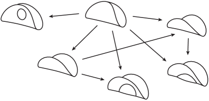
Figure 2. Some adjacencies around $B_{\infty}$

The nodal edge as a stable perturbation of the cuspidal edge is a particular case of the following construction:

Example 2.4.

One can produce map germs $f\colon(\mathbb{C}^{n},0)\to(\mathbb{C}^{n+1},0)$ with instability locus of dimension $d$ and a stable perturbation $f_{s}$ having non-trivial homology at dimension $n-d$, as follows: Choose any $\mathcal{A}$-finite unstable germ $g\colon(\mathbb{C}^{n-d},0)\to(\mathbb{C}^{n-d+1},0)$ of corank one and $g_{s}$ a stabilization of $g$. Now let $f$ and $f_{s}$ be $d$-parametric trivial unfoldings of $g$ and $g_{s}$. Since $g$ is $\mathcal{A}$-finite but not stable, it follows that the instability locus of $g$ is the origin. On the one hand, the space $T=\mathbb{C}^{d}\times\{0\}$ corresponding to the trivial parameters of $f$ must be contained in the instability locus of $f$, because it is non trivially unfolded by $f_{s}$, just as $g$ is non trivially unfolded by $g_{s}$ at the origin. On the other hand, unfoldings of stable germs are stable, because their unfoldings are also unfoldings of the original germ and hence trivial. From this it follows that the instability locus of $f$ is $T$, and that $f_{s}$ is a stabilization of $f$.

Since $(g_{s},s)$ is a stabilization of a finitely determined non stable map, the associated stable perturbation has the homotopy type of a bouquet of spheres of dimension $n-d$. Our claim follows because $(f_{s},s)$ is a trivial unfolding of $(g_{s},s)$, and therefore the image of $g_{s}$ is a deformation retract of the image of $f_{s}$.

3. Preliminaries

3.1. $\mathcal{A}$-equivalence and unfoldings

In this work, maps and (multi-)germs of maps are considered up to $\mathcal{A}$-equivalence, i.e. biholomorphisms in source and target. Standard references for this are [2] and [3].

Throughout the text, a (multi-)germ is a germ of map the form $f\colon(\mathbb{C}^{n},S)\to(\mathbb{C}^{N},y)$, where $S$ is a finite set and $f(S)=\{y\}$. Two map germs

$$f,g\colon(\mathbb{C}^{n},S)\to(\mathbb{C}^{N},0)$$

are called $\mathcal{A}$-equivalent if there exist germs of biholomorphism

$$\Phi\colon(\mathbb{C}^{n},S)\to(\mathbb{C}^{n},S),\quad\Psi\colon(\mathbb{C}^{N},0)\to(\mathbb{C}^{N},0),$$

such that the following diagram commutes:

$$\lx@xy@svg{\hbox{\raise 0.0pt\hbox{\kern 17.75703pt\hbox{\ignorespaces\ignorespaces\ignorespaces\hbox{\vtop{\kern 0.0pt\offinterlineskip\halign{\entry@#!@&&\entry@@#!@\cr&\\&\crcr}}}\ignorespaces{\hbox{\kern-17.75703pt\raise 0.0pt\hbox{\hbox{\kern 0.0pt\raise 0.0pt\hbox{\hbox{\kern 3.0pt\raise 0.0pt\hbox{$\textstyle{(\mathbb{C}^{n},S)\ignorespaces\ignorespaces\ignorespaces\ignorespaces\ignorespaces\ignorespaces\ignorespaces\ignorespaces}$}}}}}}}\ignorespaces\ignorespaces\ignorespaces\ignorespaces{}{\hbox{\lx@xy@droprule}}\ignorespaces\ignorespaces\ignorespaces{\hbox{\kern-11.05556pt\raise-20.62332pt\hbox{{}\hbox{\kern 0.0pt\raise 0.0pt\hbox{\hbox{\kern 3.0pt\hbox{\hbox{\kern 0.0pt\raise-2.39166pt\hbox{$\scriptstyle{\Phi}$}}}\kern 3.0pt}}}}}}\ignorespaces{\hbox{\kern 0.0pt\raise-30.20778pt\hbox{\hbox{\kern 0.0pt\raise 0.0pt\hbox{\lx@xy@tip{1}\lx@xy@tip{-1}}}}}}{\hbox{\lx@xy@droprule}}{\hbox{\lx@xy@droprule}}\ignorespaces\ignorespaces\ignorespaces\ignorespaces{}{\hbox{\lx@xy@droprule}}\ignorespaces\ignorespaces\ignorespaces{\hbox{\kern 24.67683pt\raise 6.1111pt\hbox{{}\hbox{\kern 0.0pt\raise 0.0pt\hbox{\hbox{\kern 3.0pt\hbox{\hbox{\kern 0.0pt\raise-1.75pt\hbox{$\scriptstyle{f}$}}}\kern 3.0pt}}}}}}\ignorespaces{\hbox{\kern 41.75703pt\raise 0.0pt\hbox{\hbox{\kern 0.0pt\raise 0.0pt\hbox{\lx@xy@tip{1}\lx@xy@tip{-1}}}}}}{\hbox{\lx@xy@droprule}}{\hbox{\lx@xy@droprule}}{\hbox{\kern 41.75703pt\raise 0.0pt\hbox{\hbox{\kern 0.0pt\raise 0.0pt\hbox{\hbox{\kern 3.0pt\raise 0.0pt\hbox{$\textstyle{(\mathbb{C}^{N},0)\ignorespaces\ignorespaces\ignorespaces\ignorespaces}$}}}}}}}\ignorespaces\ignorespaces\ignorespaces\ignorespaces{}{\hbox{\lx@xy@droprule}}\ignorespaces\ignorespaces\ignorespaces{\hbox{\kern 59.53426pt\raise-20.62332pt\hbox{{}\hbox{\kern 0.0pt\raise 0.0pt\hbox{\hbox{\kern 3.0pt\hbox{\hbox{\kern 0.0pt\raise-2.39166pt\hbox{$\scriptstyle{\Psi}$}}}\kern 3.0pt}}}}}}\ignorespaces{\hbox{\kern 59.53426pt\raise-29.5pt\hbox{\hbox{\kern 0.0pt\raise 0.0pt\hbox{\lx@xy@tip{1}\lx@xy@tip{-1}}}}}}{\hbox{\lx@xy@droprule}}{\hbox{\lx@xy@droprule}}{\hbox{\kern-17.75703pt\raise-41.24664pt\hbox{\hbox{\kern 0.0pt\raise 0.0pt\hbox{\hbox{\kern 3.0pt\raise 0.0pt\hbox{$\textstyle{(\mathbb{C}^{n},S)\ignorespaces\ignorespaces\ignorespaces\ignorespaces}$}}}}}}}\ignorespaces\ignorespaces\ignorespaces\ignorespaces{}{\hbox{\lx@xy@droprule}}\ignorespaces\ignorespaces\ignorespaces{\hbox{\kern 24.97217pt\raise-36.05914pt\hbox{{}\hbox{\kern 0.0pt\raise 0.0pt\hbox{\hbox{\kern 3.0pt\hbox{\hbox{\kern 0.0pt\raise-0.8264pt\hbox{$\scriptstyle{g}$}}}\kern 3.0pt}}}}}}\ignorespaces{\hbox{\kern 41.75703pt\raise-41.24664pt\hbox{\hbox{\kern 0.0pt\raise 0.0pt\hbox{\lx@xy@tip{1}\lx@xy@tip{-1}}}}}}{\hbox{\lx@xy@droprule}}{\hbox{\lx@xy@droprule}}{\hbox{\kern 41.75703pt\raise-41.24664pt\hbox{\hbox{\kern 0.0pt\raise 0.0pt\hbox{\hbox{\kern 3.0pt\raise 0.0pt\hbox{$\textstyle{(\mathbb{C}^{N},0)}$}}}}}}}\ignorespaces}}}}\ignorespaces. \textstyle{(\mathbb{C}^{n},S)\ignorespaces\ignorespaces\ignorespaces\ignorespaces\ignorespaces\ignorespaces\ignorespaces\ignorespaces} \scriptstyle{\Phi} \scriptstyle{f} \textstyle{(\mathbb{C}^{N},0)\ignorespaces\ignorespaces\ignorespaces\ignorespaces} \scriptstyle{\Psi} \textstyle{(\mathbb{C}^{n},S)\ignorespaces\ignorespaces\ignorespaces\ignorespaces} \scriptstyle{g} \textstyle{(\mathbb{C}^{N},0)} \textstyle{(\mathbb{C}^{n},S)\ignorespaces\ignorespaces\ignorespaces\ignorespaces\ignorespaces\ignorespaces\ignorespaces\ignorespaces} \scriptstyle{\Phi} \scriptstyle{f} \textstyle{(\mathbb{C}^{N},0)\ignorespaces\ignorespaces\ignorespaces\ignorespaces} \scriptstyle{\Psi} \textstyle{(\mathbb{C}^{n},S)\ignorespaces\ignorespaces\ignorespaces\ignorespaces} \scriptstyle{g} \textstyle{(\mathbb{C}^{N},0)}$$

Given such a germ $f\colon(\mathbb{C}^{n},0)\to(\mathbb{C}^{N},0)$ an unfolding of $f$ on $r$ parameters is a map germ

$$F\colon(\mathbb{C}^{n}\times\mathbb{C}^{r},(0,0))\to(\mathbb{C}^{N}\times\mathbb{C}^{r},(0,0)),\quad(x,u)\mapsto(f_{u}(x),u)$$

such that for $u=0$ we obtain $f_{0}=f$. Two unfoldings are called $\mathcal{A}$-equivalent as unfoldings if they are $\mathcal{A}$-equivalent via two germs of biholormorphism of the form $\Phi=\phi\times\operatorname{id}_{\mathbb{C}^{r}}$ and $\Psi=\psi\times\operatorname{id}_{\mathbb{C}^{r}}$. An unfolding $F$ of $f$ is called trivial if it is $\mathcal{A}$-equivalent, as an unfolding, to the trivial unfolding $f\times\operatorname{id}_{\mathbb{C}^{r}}$.

There are obvious analogous statements for finite maps $f\colon X\to Y$ between complex manifolds. Also, replacing biholomorphisms by homeomorphisms, we obtain the definitions of topological $\mathcal{A}$-equivalence and topologically trivial unfoldings.

Definition 3.1.

A multi-germ $f\colon(X,S)\to(Y,0),$ is stable if every unfolding $F$ of $f$ is trivial. A finite map $f\colon X\to Y$ is stable at a point $y\in Y$ if the germ $f\colon(X,f^{-1}(\{y\}))\to(Y,y)$ is stable. Finally, a finite map is stable if it is stable at every point. Topological stability is defined in the obvious analogous manner.

The instability locus $\operatorname{Inst}(f)$ of a finite map is the subspace of points $y\in Y$ where the multi-germ of $f$ at $S=f^{-1}(\{y\})$ is not stable. It is well known that $\operatorname{Inst}(f)$ is a closed complex subspace of $Y$.

Definition 3.2.

A stabilization of a germ $f$ is a one-parameter unfolding of $f$, having a representative

$$F=(f_{u},u)\colon X\times U\to Y\times U$$

so that $f_{s}$ is stable for all $s\in U\setminus\{0\}$. Topological stabilizations are defined analogously.

Let $Z=F(X\times U)$. By shrinking $X,Y$ and $U$, we may ask $F$ to satisfy the following conditions:

1. the family $\pi\colon Z\to U$ is a locally trivial fibration over $U\setminus\{0\}$,

2. the central fiber $\pi^{-1}(\{0\})$ is contractible,

3. the space $Z$ retracts onto the central fiber $f_{0}(X)$.

Such a mapping $F$ is called a good representative of the stabilization, and each of the mappings $f_{s}\colon X\to Y$ is called a stable perturbation of $f$.

It is well known that for $(n,N)$ in the nice dimensions of Mather [14], with $n<N$, all finite multi-germs admit a stabilization (observe that finite is equivalent to $\mathcal{K}$-finite whenever $n<N$). Away from the nice dimensions, every multi-germ admits a topological stabilization.

3.2. Multiple point spaces

Here we introduce the main objects needed for our result: the multiple point spaces of a finite map. Our exposition is close to [18] in spirit, but its contents can be extracted from previous work like [13].

Definition 3.3.

A strict $k$-multiple point of $f\colon X\to Y$ is a point $(x^{(1)},\dots,x^{(k)})\in X^{k}$ such that $f(x^{(i)})=f(x^{(j)})$ and $x^{(i)}\neq x^{(j)}$, for all $i\neq j$.

The $k$-th multiple point space of a stable map $f\colon X\to Y$ is the analytic closure

$$D^{k}(f)=\overline{\{\text{strict $k$-multiple points of $f$}\}}.$$

The space $D^{k}(f)$ is taken with the reduced analytic structure and the definition extends to stable multi-germs by taking representatives.

The multiple point space of a finite multi-germ $f\colon(\mathbb{C}^{n},S)\to(\mathbb{C}^{N},0)$ is

$$D^{k}(f)=D^{k}(F)\cap(\mathbb{C}^{n}\times\{0\})^{k},$$

for a stable unfolding $F\colon(\mathbb{C}^{n}\times\mathbb{C}^{r},S\times\{0\})\to(\mathbb{C}^{N}\times\mathbb{C}^{r},0)$ of $f$. The multiple point space $D^{k}(f)$ of a finite map $f\colon X\to Y$ is obtained by gluing the $k$-multiple point spaces of the multi-germs of $f$ at $f^{-1}(y)$, for all $y\in Y$. We write $D^{k}=D^{k}(f)$ whenever $f$ is understood.

For every $k$, the projection which drops the $i$-th coordinate takes strict multiple points to strict multiple points. For any finite map $X\to Y$, one can see that these projections induce maps

$$\epsilon^{i,k}\colon D^{k}\to D^{k-1}.$$

For formal reasons, it is convenient to extend this notation to the spaces $D^{1}=X$ and $D^{0}=Y$, to the maps $\epsilon^{i,2}\colon D^{2}\to X$ dropping the $i$-th coordinate, and to the map $\epsilon^{1,1}=f\colon X\to Y.$ We also write

$$\epsilon^{k}=\epsilon^{k,k}\circ\dots\circ\epsilon^{1,1}\colon D^{k}\to Y.$$

The following well known result makes precise which diagonal points are added when defining double points via passing to a stable unfolding. A proof which is consistent with this approach can be found in [18].

Lemma 3.4.

The double point space $D^{2}$ of any map $f\colon X\to Y$ consists of

1. Strict double points $(x,x^{\prime})\in X^{2}$, with $x^{\prime}\neq x$ and $f(x^{\prime})=f(x)$,

2. Diagonal singular points $(x,x)\in\Delta X$, such that $f$ is singular at $x$.

The $k$-th multiple point space $D^{k}(F)$ of a finite map $F\colon X\times U\to Y\times U$, of the form $F(x,u)=(f_{u}(x),u)$, can be embedded in $X^{k}\times U$. This embedding makes $D^{k}(F)$ into a (possibly non-flat) family of spaces $D^{k}(f_{u})$, in the sense that

$$D^{k}(f_{t}):=D^{k}(F)\cap\{u=t\}$$

In the case of corank one germs, the multiple point spaces can be computed directly without taking stable unfoldings. Every corank one map germ $(\mathbb{C}^{n},0)\to(\mathbb{C}^{p},0)$ can be taken, by a suitable change coordinates in the source and target, to a map of the form

$$f(x,u)=(f_{n}(u,x),\dots,f_{N}(u,x),u),\quad u\in\mathbb{C}^{n-1},x\in\mathbb{C}.$$

A set of generators for the ideal defining $D^{k}$ for such a map was given By Marar and Mond in [13] (see Proposition 2.16). These generators are as follows:

Lemma 3.5.

In the setting above, the multiple point space $D^{k}(f)$ is defined in $\mathbb{C}^{k}\times\mathbb{C}^{n-1}$ by the vanishing of the iterated divided differences

$$f_{j}[x_{1},x_{2},u],f_{j}[x_{1},x_{2},x_{3},u],\dots,f_{j}[x_{1},\dots,x_{k},u],\text{ for }j=n,\dots,N.$$

The divided differences are defined as

• $f_{j}[x_{1},x_{2},u]=\dfrac{f_{j}(x_{2},u)-f_{j}(x_{1},u)}{x_{2}-x_{1}}$,

• $f_{j}[x_{1},x_{2},x_{3},u]=\dfrac{f_{j}[x_{1},x_{3},u]-f_{j}[x_{1},x_{2},u]}{x_{3}-x_{2}}$

and, iteratively,

• $f_{j}[x_{1},\dots,x_{k},u]=\dfrac{f_{j}[x_{1},\dots,x_{k-2},x_{k},u]-f_{j}[x_{1},\dots,x_{k-2},x_{k-1},u]}{x_{k}-x_{k-1}},$

Having explicit generators for monogerms, we can deduce the following:

Lemma 3.6.

Let $f\colon X\to Y$ be a finite map between holomorphic manifolds of dimension $n$ and $N$ respectively. If $D^{k}$ is non-empty, then $\dim D^{k}\geq kn-(k-1)N$. If $f$ has corank one and $\dim D^{k}=kn-(k-1)N$, then $D^{k}$ is locally a complete intersection.

Definition 3.7.

We say that the multiple point space $D^{k}$ of map $f\colon X\to Y$ as above has the expected dimension if it is empty or has dimension $kn-(k-1)N$. A map is called dimensionally correct if all its multiple point spaces have the expected dimension.

Observe that, to check if a finite map is dimensionally correct, it is enough to check dimensions from $D^{2}$ to the smallest $k$ such that $D^{k}=\emptyset$. This is because $D^{k}=\emptyset$ forces the higher multiplicity spaces to be empty, and hence to have the expected dimension.

We gather some results from [6] and [13] describing the relation between stability and multiple point spaces in the corank one setting.

Theorem 3.8.

A corank one map $f$ is stable if and only if every $D^{k}$ is smooth of dimension $kn-(k-1)N$ or empty. In this case, the following properties are satisfied:

1. Every $D^{k}$ is the closure of the set of strict $k$-multiple points.

2. The maps $\epsilon^{i,k}\colon D^{k}\to D^{k-1}$ are corank one stable maps.

3. The multiple point spaces satisfy the iteration principle

   $$D^{k}(\epsilon_{r})\cong D^{r+k-1},$$

   via isomorphisms which commute with the maps $D^{r}(\epsilon_{k})\to D^{r-1}(\epsilon_{k})$ and $D^{r+k}\to D^{r+k-1}$.

Lemma 3.9.

For every finite map $f$, the maps $\epsilon^{i,k}\colon D^{k}\to D^{k-1}$ and $\epsilon^{k}\colon D^{k}\to Y$ are finite.

Proof.

It suffices to show the claim for $\epsilon^{i,k}$, because every $\epsilon^{k}$ is a composition of those. Recall that the spaces $D^{k}$ are obtained by glueing the corresponding spaces for representatives of multi-germs at $S=f^{-1}(\{y\})$, and thus it suffices to show the claim for multi-germs. Observe that the restriction of a finite map is finite and the maps $\epsilon^{i,k}$ are restrictions of those of any unfolding. Hence, since every finite multi-germ admits a stable unfolding, we may assume that $f$ is a stable finite multi-germ. In this case, the maps $D^{k}\to D^{k-1}$ are stable maps from a manifold of dimension $kn-(k-1)N$ to another of dimension $(k-1)n-(k-2)N$, hence finite. ∎

Corollary 3.10.

Let $X$ and $Y$ be complex manifolds of dimension $n$ and $N$ respectively. For any finite and dimensionally correct corank one map $f\colon X\to Y$, with instability locus of dimension $d$, the spaces $D^{k}$ are locally complete intersections of dimension $kn-(k-1)N$, if not empty, with singular locus of dimension at most $d$.

Corollary 3.11.

For any finite dimensionally correct corank one map $f\colon X\to Y$ as above, the union of the projections to $X$ of the singular loci of the $D^{k}$ is equal to the instability locus of $f$. In particular, if the instability locus has dimension $d$, then there is at least one space $D^{k}$ having a $d$-dimensional singular locus.

4. Milnor fibrations and disentanglements

In this section we shall discuss two setups in parallel which may be seen as two branches of a common theoretical trunk: Smoothings of non-isolated singularities and disentanglements for finite map germs. Both setups fit into the commutative diagram (2) below: In the first case we consider $(Z_{0},0)\subset(\mathbb{C}^{N},0)$ as a non-isolated singularity and $(Z_{0},0)\hookrightarrow(Z,0)\overset{h}{\longrightarrow}(\mathbb{C},0)$ a smoothing of it over $(\mathbb{C},0)$ with total space $(Z,0)$. In the other case, $(Z_{0},0)$ appears as the image of a finite holomorphic map germ $f\colon(\mathbb{C}^{n},0)\to(\mathbb{C}^{N},0)$. Passing to an unfolding $F\colon(\mathbb{C}^{n},0)\times(\mathbb{C},0)\to(\mathbb{C}^{N},0)\times(\mathbb{C},0)$, we can easily verify that also $F$ is finite and hence has an analytically closed image $(Z,0)\subset(\mathbb{C}^{N+1},0)$ equipped with a projection $h$ to the base of the unfolding. Forgetting about $F$ we obtain a deformation of $(Z_{0},0)$ over $(\mathbb{C},0)$ in the classical sense.

(2)

We will usually write $y$ for the standard coordinates of $(\mathbb{C}^{N},0)$ and $(y,u)$ for those of $(\mathbb{C}^{N+1},0)$ with $u$ the deformation parameter. The function $h$ is the restriction of $u$ to the total space $(Z,0)$ of the deformation.

4.1. The fibration theorems

Next, we will make precise what we understand to be the Milnor fiber in this situation closely following [12]. By abuse of notation we will denote by $Z_{0}$, $Z$, and $h$ a set of representatives of the corresponding germs defined on some product $Y\times\Delta\subset\mathbb{C}^{N+1}=\mathbb{C}^{N}\times\mathbb{C}$ with $Y$ an open neighborhood of $0$ in $\mathbb{C}^{N}$ and $\Delta$ an open disc around the origin in the deformation base $\mathbb{C}$.

One starts out by endowing $(Z,0)$ with a Whitney stratification $\Sigma=\{S_{\alpha}\}_{\alpha\in A}$, in which $(Z_{0},0)$ appears as union of strata. For the existence of complex analytic Whitney stratifications see e.g. [21]. If (2) is a smoothing of $(Z_{0},0)$, then $Z\setminus Z_{0}$ is itself necessarily smooth in a neighborhood of the origin and in this case we have a unique open stratum which we will call $S_{0}:=Z\setminus Z_{0}$. Whenever (2) arises from an unfolding $F:(\mathbb{C}^{n}\times\mathbb{C},0)\to(\mathbb{C}^{N}\times\mathbb{C},0)$ of a finite holomorphic map germ $f=f_{0}:(\mathbb{C}^{n},0)\to(\mathbb{C}^{N},0)$, the open stratum $S_{0}$ might not coincide with $Z\setminus Z_{0}$, since the deformation of the image $(Z_{0},0)$ induced from the unfolding $F$ does not have to be a smoothing of $(Z_{0},0)$. In either case we may utilize the Curve Selection Lemma to verify that the restriction of $h$ to any stratum $S_{\alpha}$ outside $Z_{0}$ does not have a critical point in a neighborhood of $0\in Z$. After shrinking our representatives, we may therefore assume that $h|_{S_{\alpha}}$ is a submersion at any point $p\in S_{\alpha}$, $p\notin Z_{0}$ and write

$$T_{p}h^{-1}(\{h(p)\})=\ker\operatorname{d}\!h|_{S_{\alpha}}\subset T_{p}S_{\alpha}$$

for the tangent space of its fiber $h^{-1}(\{h(p)\})$ through $p$. Note that by construction the restriction of $h$ to any stratum $S_{\alpha}\subset Z_{0}$ in the central fiber is the constant map. Therefore at any point $p\in S_{\alpha}\subset Z_{0}$ the spaces $T_{p}S_{\alpha}$ and $T_{p}h^{-1}(\{h(p)\})$ coincide.

As a second step one refines the stratification in order to also fulfill Thom’s $a_{h}$-condition. This is the crucial ingredient in order to establish the fibration theorems, see [20]. The existence of such refinements in the complex analytic setting has been shown in [9].

Definition 4.1.

Let $h\colon(Z,p)\to(\mathbb{C},q)$ be a holomorphic map germ and $\Sigma=\{S_{\alpha}\}_{\alpha\in A}$ a Whitney stratification of $(Z,p)$ as above. Consider a sequence of points $(p_{i})_{i\in\mathbb{N}}$ in a stratum $S_{\alpha}$ converging to $p\in S_{\beta}$ such that the sequence of tangent spaces

$$T_{p_{i}}S_{\alpha}\overset{n\to\infty}{\longrightarrow}T_{\infty}\supset T_{p}S_{\beta}$$

also converges. From this one also obtains the sequence of relative tangent spaces

$$K_{i}:=T_{p_{i}}h^{-1}(\{h(p_{i})\})\subset T_{p_{i}}S_{\alpha}.$$

Passing to a subsequence, we may assume that also the $K_{i}$ converge to a limit $K_{\infty}\subset T_{\infty}$. We say that the stratification $\Sigma$ satisfies the $a_{h}$-condition at $p$, if for any such sequence one has

(3) $$K_{\infty}\supset T_{p}h^{-1}\left(\{h(p)\}\right)$$

where $T_{p}h^{-1}(\{h(p)\})=\ker\operatorname{d}\!h|_{S_{\beta}}(p)\subset T_{p}S_{\beta}$.

In a third step we restrict to proper representatives by choosing a Milnor ball. Suppose

$$F=(f_{u},u):X\times\Delta\to\mathbb{C}^{N}\times\Delta$$

is a representative of the unfolding $F$ as above defined on some open neighborhood $X\subset\mathbb{C}^{n}$ over a small disc $\Delta\subset\mathbb{C}$. Let $F(X)$ be its image in $\mathbb{C}^{N}$. We may choose the open neighborhood $0\in Y\subset\mathbb{C}^{N}$ such that $Z:=F(X)\cap Y\times\Delta$ is analytically closed in $Y\times\Delta$. A Milnor ball is now chosen as follows: Consider the squared distance function from the $u$-axis in $\mathbb{C}^{N+1}$

$$\rho:(y,u)\mapsto|y|^{2}.$$

This is a real analytic function. We can apply the Curve Selection Lemma to deduce that $\rho$ has no critical values on some small interval $(0,\varepsilon_{0}]$ with respect to the stratification $\Sigma$ in a neighborhood of the origin. We may assume this neighborhood to be $Y\times\Delta$ again. Consequently,

$$\overline{Z}:=Z\cap\rho^{-1}([0,\varepsilon_{0}])\quad\textnormal{ and }\quad\overline{Z}_{0}:=Z_{0}\cap\rho^{-1}([0,\varepsilon_{0}])$$

are again Whitney stratified spaces. Let

$$\partial\overline{Z}:=Z\cap\rho^{-1}(\{\varepsilon_{0}\})\quad\textnormal{ and }\quad\partial\overline{Z}_{0}:=Z_{0}\cap\rho^{-1}(\{\varepsilon_{0}\})$$

be their boundaries. They inherit a Whitney stratification $\partial\Sigma$ from $\Sigma$ by intersecting each stratum $S_{\alpha}$ with $\rho^{-1}(\{\varepsilon_{0}\})$. Moreover, the restriction

$$h|_{\overline{Z}}:\overline{Z}\to\Delta$$

is proper and, as a consequence of Thom’s first Isotopy Lemma applied to $\rho$ on $Z_{0}$, one has:

Corollary 4.2 (Conical structure).

The inclusion $\{0\}\hookrightarrow\overline{Z}_{0}$ is a deformation retract.

In this setup, Lê provided the following fibration theorem, cf. [12], Theorem 1.1 and Remark 1.3 (b):

Theorem 4.3.

There exists $\varepsilon_{0}\gg\eta>0$ such that the restriction

$$h:\overline{Z}\cap h^{-1}(\Delta_{\eta}\setminus\{0\})\to\Delta_{\eta}\setminus\{0\}$$

is a topological fibration, where $\Delta_{\eta}$ is the disc around the origin of radius $\eta$.

Definition 4.4.

In a given deformation of a space $(Z_{0},0)$ as in (2) and Theorem 4.3, we call

$$h^{-1}(\{t\})\cap\overline{Z},\quad t\in\Delta_{\eta}\setminus\{0\}$$

the Milnor fiber of $h$ on $(Z,0)$. If (2) arises from a stabilization $F$ of a holomorphic map germ $f$, then we will speak of the disentanglement of $f(X)$ in the given unfolding $F$.

The reader should verify that with the particular choices for our representatives made in this section, the requirements on a good representative in Definition 3.2 are indeed satisfied.

Remark 4.5.

The notions of this section are mostly of topological nature. A priori, the space germs $(Z,0)$, and $(Z_{0},0)$ are germs of complex spaces, i.e. they might have a non-reduced scheme structure. However, when considering their Whitney stratifications, we only consider their reduced models and the reduced structure of the strata and consequently everything that follows is to be understood purely topologically.

4.2. Induced deformations of multiple point spaces

In the setting we will encounter when dealing with the multiple point spaces, we do not have the freedom to choose the shape of $\overline{Z}$ inside $Z$ since multiple point spaces and their deformations appear as preimages of the canonical projections to the unfolding of the original map germ, which had been chosen beforehand: Suppose as usual that we are given a representative

$$F=(f_{u},u):X\times\Delta\to Y\times\Delta\subset\mathbb{C}^{N}\times\mathbb{C}$$

of an unfolding of a finite holomorphic map germ $f=f_{0}$. Let $Z\subset Y\times\Delta$ be its image and $D^{k}$ the multiple point spaces:

(4)

Consider the squared distance $\rho$ from the $u$-axis in $\mathbb{C}^{N+1}$ as before. On all the spaces $D^{k}$ this already fixes the function with respect to which our proper representatives are about to be chosen:

(5) $$\rho_{k}:=\rho\circ\varepsilon^{k}:D^{k}\to\mathbb{R}$$

From the finiteness and analyticity of all the maps $\varepsilon^{k}$ we easily deduce the following three properties of all the $\rho_{k}$:

1. $\rho_{k}$ has an isolated zero on the central fibers $D^{k}_{0}=D^{k}\cap\{u=0\}$, resp. $Z\times\{0\}$, at the origin.

2. There exists $\varepsilon_{0}>0$ such that for each $0<\varepsilon\leq\varepsilon_{0}$ and all $k>0$ the restriction

   $$u:\overline{D}^{k}=D^{k}\cap\rho_{k}^{-1}([0,\varepsilon_{0}])\to\Delta$$

   is proper.

3. Furthermore, $\varepsilon_{0}>0$ can be chosen small enough such that each $\rho_{k}$ is a stratified submersion on $D_{0}^{k}\cap\rho_{k}^{-1}((0,\varepsilon_{0}])$.

We will from now on assume that $\varepsilon_{0}$ has been chosen small enough to fulfill all these requirements simultaneously with those formulated in the previous section.

Recall Theorem 3.8, Corollary 3.10, and Corollary 3.11: If (4) is a stabilization of a dimensionally correct map germ $f_{0}$ of corank one with instability locus of dimension $d=\dim\operatorname{Inst}(f_{0})$, then the induced deformations

$$\overline{D}^{k}\overset{u}{\longrightarrow}\Delta$$

are smoothings of the complete intersection singularities

$$(D^{k}_{0},0)=(D^{k}\cap\{u=0\},0),$$

which have non-isolated singular locus of dimension at most $d$. The only difference to the classical case is the unconventional choice of the Milnor balls via the functions $\rho_{k}$. But as we shall see below, this does not alter the theory and we can apply the usual machinery to get to know their topological invariants. The induced deformation of one of the multiple point schemes is what the reader should have in mind when progressing to the next section.

4.3. Non-isolated complete intersection singularities

Suppose we are given a smoothing of a nonisolated singularity $(Z_{0},0)\subset(\mathbb{C}^{N},0)$ as in (2). There are essentially two different ways to construct transversal, isolated singularities from nonisolated ones. In the first case one considers the singular part of the link $\partial\overline{Z}_{0}=\rho^{-1}(\{\varepsilon_{0}\})\cap Z_{0}$ as e.g. in [19] and also the original work by Kato and Matsumoto [11]. In the other case, which is for example exhibited in [12], one takes hyperplane slices at the central point $0\in Z_{0}$, which are transverse to the singular locus. A detailed description of the sense of transversality underlying this choice is outlined in [8, Section 2]. Unfortunately, the article only deals with hypersurfaces, but the methods applied there carry over naturally: We are considering functions $h\colon(Z,0)\to(\mathbb{C},0)$ on an arbitrary reduced, complex analytic space $(Z,0)\subset(\mathbb{C}^{N+1},0)$, rather than functions on smooth spaces. All the choices of stratifications and their refinements in [8] can easily be adapted to the situation in Diagram (2) and one eventually obtains the following theorem by Lê, [12], Theorem 2.1:

Theorem 4.6.

There is an open Zariski dense set $\Omega$ in the space of affine hyperplanes of $\mathbb{C}^{N}$ at $0$ such that if $l=0$ belongs to $\Omega$, there exists an analytic curve $C_{0}\subset W\subset\mathbb{C}^{2}$ in an open neighborhood $W$ of $0\in\mathbb{C}^{2}$, such that for any $\varepsilon>0$ small enough and $\eta>0$, $\varepsilon\gg\eta$, the mapping

$$(h,l):Z\cap B_{\varepsilon}\cap(h,l)^{-1}(B_{\eta}\setminus C_{0})\to B_{\eta}\setminus C_{0}$$

is a topological fibration.

As usual, $B_{\varepsilon}$ and $B_{\eta}$ denote the balls of radius $\varepsilon$ and $\eta$ in $\mathbb{C}^{N}$ and $\mathbb{C}^{2}$ respectively. It is evident from the proof that we can replace $B_{\varepsilon}$ by $\rho_{k}^{-1}([0,\varepsilon])$ for a suitable real analytic function $\rho_{k}$, which fulfills the requirements formulated in Section 4.2. The verification of this fact along the lines of [12] is left to the reader. See also [8].

The curve $C_{0}$ is the image of the so-called Polar curve of the linear form $l$ relative to $h$ on $Z$:

(6) $$\Gamma=\overline{\{y\in Z\setminus Z_{0}:\ker\operatorname{d}\!h(y)\subset\{l=0\}\}}.$$

For a fixed value $t\in\mathbb{C}$, $|t|$ small enough, the restriction of $l$ to the interior of $\overline{Z}_{t}=\rho^{-1}([0,\varepsilon])\cap h^{-1}(\{t\})$ has only isolated critical points – the intersection points of $\Gamma$ with $h^{-1}(\{t\})$. One can furthermore show (see [8]) that for a generic choice of $l$ these critical points are Morse critical points. But we shall not need that fact.

What is more important for our purposes, is the fact that the set $\Omega$ of admissible hyperplanes $L=\{l=0\}$ is Zariski open. Let $\Omega^{\prime}$ be the set of hyperplanes, which are transversal to the stratification $\Sigma$ of the total space $Z$ at $0$. By this we mean that the restriction of the linear form $l$ to any stratum of positive dimension is a submersion and that at an arbitrary point $p\in Z$ it does not annihilate any limiting tangent space of adjacent strata. Since the intersection of two Zariski open sets is again Zariski open and in particular non-empty, we may choose $L\in\Omega\cap\Omega^{\prime}$. With this choice it is easy to see that, since $Z_{0}$ is a union of strata, the transversal singularity given by

(7) $$Z_{0}^{\pitchfork}:=Z_{0}\cap L$$

is nonsingular at every nonsingular point of $Z_{0}$. Moreover, $l$ is a non-constant function on every irreducible component of any stratum $S_{\beta}\subset\operatorname{Sing}(Z_{0})$ of positive dimension and hence $\dim\operatorname{Sing}(Z_{0}^{\pitchfork})=\dim\operatorname{Sing}(Z_{0})-1$, whenever $Z_{0}$ has non-isolated singularities. This yields an induction argument on $d=\dim\operatorname{Sing}(Z_{0})$:

Theorem 4.7.

Suppose $h:(Z,0)\to(\mathbb{C},0)$ as in (2) is a smoothing of an $n$-dimensional, non-isolated singularity $(Z_{0},0)\subset(\mathbb{C}^{N},0)$ with singular locus $\operatorname{Sing}(Z_{0})$ of dimension $d$ at $0$ and $L=\{l=0\}$ is a hyperplane meeting the requirements of Theorem 4.3 with transversal singularity $(Z_{0}^{\pitchfork},0)$. Let $\rho$ be a non-negative real analytic function on a neighborhood of the origin in $\mathbb{C}^{N}$, which defines a good proper representative $h:\overline{Z}\to\Delta$ of the deformation of $\overline{Z}_{0}=h^{-1}(\{0\})\cap\rho^{-1}([0,\varepsilon])$ and the associated transversal singularity $\overline{Z}_{0}^{\pitchfork}$. Then up to homotopy we obtain the space $\overline{Z}_{t}$ from $\overline{Z}_{t}^{\pitchfork}$ by attaching handles of real dimension $n$.

The idea behind the proof of this theorem is to use the squared distance function $\lambda:=|l|^{2}$ from the hyperplane $L$ as a real Morse function on $\overline{Z}_{t}$. The latter is a manifold with boundary and we therefore have to pass to stratified Morse theory. Perturbing the equation $l$ slightly, we may assume that the complex function $l$ has only Morse critical points on the interior of $\overline{Z}_{t}\setminus\overline{Z}_{0}^{\pitchfork}$ and it is easily seen that outside $L\cap\overline{Z}_{t}$, the function $\lambda$ has real Morse singularities of index $n=\dim_{\mathbb{C}}\overline{Z}_{t}$ precisely at the critical points of $l$. The difficulty in the proof does therefore not arise from the critical points of $\lambda$ in the interior of $\overline{Z}_{t}\setminus\overline{Z}_{0}^{\pitchfork}$, but from critical points of $\lambda$ on the boundary $\partial\overline{Z}_{t}$. More precisely: The hardest part of the proof is to show that these critical points do not contribute to changes in the homotopy type when passing through their associated critical values.

In order to understand why this is the case, recall the following notions of Morse theory on manifolds with boundary. Let $f\colon M^{\prime}\to\mathbb{R}$ be a smooth function on a manifold $M^{\prime}$ and let $M\subset\overline{M}\subset M^{\prime}$ be an open submanifold with boundary $\partial M$. For a point $p\in\partial M$ choose a smooth function $t\colon(M^{\prime},p)\to(\mathbb{R},0)$ defining the boundary, i.e.

$$(\partial\overline{M},p)=(t^{-1}(\{0\}),p)\quad\textnormal{and}\quad(\overline{M},p)=(t^{-1}((-\infty,0]),p).$$

Definition 4.8.

We say that $p\in\partial M$ is a boundary critical point for $f$ on $\overline{M}$, if $p$ is a regular point of $f$ on $M^{\prime}$ and a critical point of the restriction $f|_{\partial M}$, i.e. if in the tangent space $T_{p}M^{\prime}$ the equation

(8) $$\operatorname{d}\!f(p)=a\cdot\operatorname{d}\!t(p)$$

holds for some $a\neq 0$. The point $p$ is an outward (resp. inward) critical point of $f$ on $\overline{M}$ if the coefficient $a$ in (8) is positive (resp. negative). Moreover, a boundary critical point $p$ is a Morse point if the restriction $f|_{\partial\overline{M}}$ has a Morse critical point at $p$.

The following lemma can easily be deduced from stratified Morse theory, see [4].

Lemma 4.9.

Let $f\colon M^{\prime}\to\mathbb{R}$ be a smooth function on a manifold $M^{\prime}$ and $M\subset\overline{M}\subset M^{\prime}$ a submanifold with boundary $\partial\overline{M}$ such that the restriction of $f$ to $\overline{M}$ is proper. Suppose $p\in\partial\overline{M}$ is a boundary Morse critical point with critical value $b\in\mathbb{R}$ and no further critical points in the fiber $\overline{M}\cap f^{-1}(\{b\})$.

If $p$ is an outward critical point of $f$, then there exists an $\varepsilon>0$ such that the space $f^{-1}((-\infty,b-\varepsilon])$ is a strong deformation retract of $f^{-1}((-\infty,b+\varepsilon])$.

If $p$ is an inward critical point of $f$, then up to homotopy we obtain $f^{-1}((-\infty,b+\varepsilon])$ from $f^{-1}((-\infty,b-\varepsilon])$ by attaching a cell of dimension $i$, where $i$ is the Morse index of the restriction $f|_{\partial\overline{M}}$.

Example 4.10.

Consider “Kenny’s head” (Figure 3), the manifold $\overline{M}$ given by the intersection of the sphere $S^{2}\subset\mathbb{R}^{3}$ with the half space $\{y\leq 1/\sqrt{2}\}$. As usual we take the height function $z$ as a Morse function on $M$. There are four critical points of $z$ on $\overline{M}$: Two on the interior of $\overline{M}$ inside Kenny’s throat and on the top of his head and two boundary critical points close to his chin and on his forehead. Consider the spaces

$$\overline{M}_{c}:=z^{-1}((-\infty,c])\cap\overline{M}$$

for varying $c$. It is easily seen that passing through the critical value $-1/\sqrt{2}$ of the boundary critical point at Kenny’s chin does not change the homotopy type of $\overline{M}_{c}$. Indeed, this is an outward critical point.

On the other hand, when we approach $c=1/\sqrt{2}$, the critical value coming from the critical point on the forehead, we attach a $1$-cell to $\overline{M}_{c-\varepsilon}$. This is the case, because the critical point on the forehead is inward pointing and the Morse index of the restriction of $z$ to $\partial\overline{M}$ is $1$.

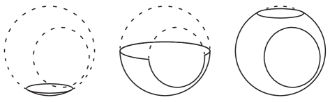
Figure 3. Slicing Kenny’s head.

Lemma 4.11.

In the setting of Theorem 4.7, let $\lambda=|l|^{2}$ be the squared distance from $L$. We say that $p\in\partial\overline{Z}\cap h^{-1}(\Delta_{\delta}\setminus\{0\})$ is a relative boundary critical point of $\lambda$, if it is a boundary critical point on the fiber

$$\overline{Z}_{t}=h^{-1}(\{h(p)\})\cap\rho^{-1}([0,\varepsilon])$$

of $h$ over $t=h(p)$. We can choose an $\varepsilon>0$ small enough such that

1. there are no relative boundary critical points in a neighborhood of $\partial\overline{Z}_{0}^{\pitchfork}$;

2. there exists a $\delta>0$ such that whenever $p\in\partial\overline{Z}$ is a relative boundary critical point, then it is an outward critical point of $\overline{Z}_{h(p)}$.

From the proof of this lemma we first extract a further technicality as a statement of its own.

Lemma 4.12.

Let $V$ be a finite dimensional vector space over a field $\mathbb{K}$ with $\mathbb{K}=\mathbb{R}$ or $\mathbb{C}$. Let $(W_{n})_{n\in\mathbb{N}}$ be a sequence of subspaces in $V$ converging to a limit space $W$ and let $(\Phi_{n})_{n\in\mathbb{N}}$ and $(\Psi_{n})_{n\in\mathbb{N}}$ be linear forms on $V$ converging to linear forms $\Phi$ and $\Psi$ respectively with $\Psi\neq 0$. Suppose we have for each $n\in\mathbb{N}$

$$\Phi_{n}|_{W_{n}}=a_{n}\cdot\Psi_{n}|_{W_{n}}$$

for some sequence of numbers $(a_{n})_{n\in\mathbb{N}}$ in $\mathbb{K}$. Then $(a_{n})_{n\in\mathbb{N}}$ converges to some $a\in\mathbb{K}$ and

$$\Phi|_{W}=a\cdot\Psi|_{W}.$$

Proof.

Let $v\in W$ be a vector with $\Psi(v)\neq 0$ and choose a sequence of vectors $(v_{n})_{n\in\mathbb{N}}$ with $v_{n}\in W_{n}$ and $\lim_{n\to\infty}v_{n}=v$. Then due to continuity

$$a_{n}\cdot\Psi_{n}(v_{n})=\Phi_{n}(v_{n})\overset{n\to\infty}{\longrightarrow}\Phi(v)=a\cdot\Psi(v)$$

for some $a\in\mathbb{K}$. We immediately deduce that for $n$ big enough

$$a_{n}=\frac{\Phi_{n}(v_{n})}{\Psi_{n}(v_{n})}\overset{n\to\infty}{\longrightarrow}\frac{\Phi(v)}{\Psi(v)}=a,$$

so in particular $(a_{n})_{n\in\mathbb{N}}$ converges. It follows a posteriori that therefore also

$$\Phi|_{W}=a\cdot\Psi|_{W}$$

as linear forms on $V$. ∎

Proof.

(of Lemma 4.11) We may choose the representative $Z$ so that we can assume that $h$ has no critical points on $Z$ outside $Z_{0}$ and also $\rho$ does not have critical points on $Z$ outside $\{\rho=0\}$. Since $Z_{0}$ is a union of strata and the hyperplane $L$ is chosen transversal to the stratification, this holds in particular for $Z_{0}$ and $Z_{0}^{\pitchfork}$. For a point $p\in S_{\alpha}\subset Z$ let $Z_{h(p)}=h^{-1}(\{h(p)\})$ be the fiber of $h$ through this point. We denote its tangent space by

$$K(p)=\ker\operatorname{d}\!h|_{S_{\alpha}}(p)=T_{p}h^{-1}(\{h(p)\})=T_{p}Z_{h(p)}.$$

In particular $K(p)=T_{p}S_{\alpha}$, whenever $p\in Z_{0}$, since $h$ is constant on $Z_{0}$. The $a_{h}$-condition moreover assures that for any sequence of points $(p_{n})_{n\in\mathbb{N}}\subset S_{\alpha}$ converging some $p\in S_{\beta}$ one has

$$\lim_{n\to\infty}K(p_{n})\supset K(p)$$

whenever the limit exists.

We first show $i)$. Certainly $\operatorname{d}\!\lambda(p)=0$ at any $p\in L$. However, by the choice of $L$ and $\varepsilon$ with respect to $Z$ we have that for any $p\in\partial\overline{Z}_{0}^{\pitchfork}$, $p\in S_{\beta}\subset Z_{0}$, the real differentials

$$\Re\operatorname{d}\!l(p),\quad\Im\operatorname{d}\!l(p),\quad\textnormal{and}\quad\operatorname{d}\!\rho(p)$$

are linearly independent over $\mathbb{R}$ on $T_{p}S_{\beta}$. This is equivalent to saying that

$$\operatorname{d}\!l(p)\quad\textnormal{ and }\quad\operatorname{d}\!^{1,0}\rho(p)$$

are linearly independent over $\mathbb{C}$, where $\operatorname{d}\!^{1,0}\rho(p)$ is the holomorphic part of the differential of $\rho$ considered as a map to $\mathbb{C}$. Now suppose there was a sequence $(p_{n})_{n\in\mathbb{N}}$ of points in some adjacent stratum $S_{\alpha}$ converging to $p$ and such that at each $p_{i}$ one has

$$\operatorname{d}\!l(p_{n})|_{K(p_{n})} = c_{n}\cdot\operatorname{d}\!^{1,0}\rho(p_{n})|_{K(p_{n})}$$

for some sequence of complex numbers $c_{n}$. Passing to a subsequence, if necessary, we may assume that the limit $\lim_{n\to\infty}K(p_{n})=K$ exists. Applying Lemma 4.12 we obtain a contradiction to the linear independence of $\operatorname{d}\!l(p)$ and $\operatorname{d}\!^{1,0}\rho(p)$ on $T_{p}S_{\beta}\subset K$. We infer that there exists an open neighborhood $U$ of $\partial\overline{Z}_{0}^{\pitchfork}$ in $Z$ such that for each stratum $S_{\alpha}$ and every point $q\in U\cap S_{\alpha}$ the differentials $\operatorname{d}\!l(q)$ and $\operatorname{d}\!^{1,0}\rho(q)$ are linearly independent over $\mathbb{C}$.

It is now easy to see from the formula

$$\operatorname{d}\!\lambda=2\Re(\overline{l}\cdot\operatorname{d}\!l)$$

that on this open neighborhood also $\operatorname{d}\!\lambda$ and $\operatorname{d}\!\rho$ must be linearly independent, whenever $\overline{l}\neq 0$, i.e. outside $L$. The points on $L\cap\overline{Z}\cap U$ on the other hand cannot be relative boundary critical points, since they are critical points of $\lambda$ on the fiber $Z_{t}$ already.

Concerning $ii)$: It has been shown in [22], Lemma 2.3.8, that we can choose $\varepsilon>0$ small enough such that on $\overline{Z}_{0}$ the following holds: Whenever in a point $p\in\partial\overline{Z}_{0}$, $p\in S_{\beta}$, we have a linear dependence

(9) $$\operatorname{d}\!\lambda(p)|_{T_{p}S_{\beta}}=a\cdot\operatorname{d}\!\rho(p)|_{T_{p}S_{\beta}},$$

then $a\geq 0$ with equality if and only if $p\in\partial\overline{Z}_{0}^{\pitchfork}$.

We briefly recall the argument. It can be shown that

$$C^{-}=\overline{\{p\in\partial\overline{Z}_{0}:\operatorname{d}\!\lambda(p)|_{T_{p}S_{\beta}}=a\cdot\operatorname{d}\!\rho(p)|_{T_{p}S_{\beta}},a<0\}}$$

is a real semi-analytic set. If the point $0\in Z$ was in $C^{-}$, then we can choose a real analytic path $\gamma:[0,t_{1})\to C^{-}$ with $\gamma(0)=0$ and $\gamma(t)\notin C^{-}\cap L$ for all $0<t<t_{1}$. Comparing the integrals

$$\lambda(\gamma(t))=\int_{0}^{t}\operatorname{d}\!\lambda(\gamma(\tau))\dot{\gamma}(\tau)\operatorname{d}\!\tau\quad\textnormal{ and }\quad\rho(\gamma(t))=\int_{0}^{t}\operatorname{d}\!\rho(\gamma(\tau))\dot{\gamma}(\tau)\operatorname{d}\!\tau$$

we see that

$$a(\tau)=\frac{\operatorname{d}\!\lambda(\gamma(\tau))\dot{\gamma}(\tau)}{\operatorname{d}\!\rho(\gamma(\tau))\dot{\gamma}(\tau)}$$

has a Laurent expansion at $\tau=0$ and hence either $a(\tau)$ or $1/a(\tau)$ extends to a real analytic function $\alpha$ on $[0,t_{1})$. Since both $\lambda$ and $\rho$ only assume non-negative values, the leading coefficient of this function must be positive – a contradiction to $a<0$ in the construction of $C^{-}$.

We can now finish the proof of $ii)$. Suppose there exists a point $p\in\partial\overline{Z}_{0}$, which is the limit point of a sequence $(p_{n})_{n\in\mathbb{N}}$ of relative boundary critical points in the open stratum $S_{0}$. Then at each point $p_{n}$ we have

$$\operatorname{d}\!\lambda(p_{n})|_{T_{p_{n}}S_{0}}=a_{n}\cdot\operatorname{d}\!\rho(p_{n})|_{T_{p_{n}}S_{0}}$$

with $a_{n}\leq 0$. Another application of Lemma 4.12 shows that in this case we would have

$$\operatorname{d}\!\lambda(p)|_{T_{p}S_{\alpha}}=a\cdot\operatorname{d}\!\rho(p)|_{T_{p}S_{\alpha}},$$

$S_{\alpha}$ the stratum containing $p$ and $a=\lim_{n\to\infty}a_{n}\leq 0$. If $a<0$ this is a contradiction to (9). If $a=0$, then $\operatorname{d}\!\lambda(p)=0$. But then $p\in L$ and we saw in $i)$ that $p$ cannot be a limit of relative boundary critical points.

We deduce that there exists an open neighborhood $V$ of $\partial\overline{Z}_{0}$ in $Z$ such that no point in $V$ is a relative inward boundary critical point. Choose $\delta>0$ small enough such that $\partial\overline{Z}\cap h^{-1}(\Delta_{\delta})$ is contained in $V$.

∎

Proof.

(of Theorem 4.7) Fix an $\varepsilon>0$ and choose $\delta>0$ as in Lemma 4.11. Choose $t\in\Delta_{\delta}$, $t\neq 0$ and consider $\lambda=|l|^{2}$ on $\overline{Z}_{t}$.

Taking a slight perturbation $\tilde{l}$ of the equation $l$, we may assume that $\tilde{\lambda}=|\tilde{l}|^{2}$ is a Morse function on the manifold with boundary $\overline{Z}_{t}$, see [4][Chapter 1, Example 2.2.4]. We may also choose a regular value $l_{0}$ of $\tilde{l}$ on $\overline{Z}_{t}$ close to $0$ and recenter $\tilde{l}$ at $l_{0}$ so that $\overline{Z}_{t}^{\pitchfork}$ is smooth, while retaining the Morse properties. Furthermore, since all the boundary critical points of $\lambda$ on $\overline{Z}_{t}$ were outward and $\tilde{\lambda}$ can be chosen arbitrarily close to $\lambda$ in the Whitney topology of smooth functions, also the boundary critical points of $\tilde{\lambda}$ are outward. With these choices we replace $l$ by $\tilde{l}$ and $\lambda$ by $\tilde{\lambda}$ in what follows.

Since $l:\overline{Z}_{t}\to\mathbb{C}$ is proper, the set of critical values is closed and we find $\eta>0$ such that

$$l\colon l^{-1}(\overline{\Delta}_{\eta})\cap\overline{Z}_{t}\to\overline{\Delta}_{\eta}$$

is a trivial bundle $\lambda^{-1}([0,\eta])\cap\overline{Z}_{t}\cong\overline{Z}_{t}^{\pitchfork}\times\Delta_{\eta}$. For any $c\in[\eta,\infty)$ denote $\overline{Z}_{t}\cap\lambda^{-1}([0,c])$ by $\overline{Z}_{t}^{\leq c}$.

As remarked earlier, the real valued function $\lambda$ has real Morse singularities of index $n=\dim_{\mathbb{C}}\overline{Z}_{t}$ at each of the complex Morse points of $l$ in the interior of $\overline{Z}_{t}$. Consequently, up to homotopy, we attach an $n$-cell to $\overline{Z}_{t}^{\leq c}$ each time $c$ passes through one of the critical values of these points. On the other hand, whenever $c$ crosses a critical value of a boundary critical point $p\in\partial\overline{Z}_{t}$, the homotopy type of $\overline{Z}_{t}^{\leq c}$ does not change according to Lemma 4.9, because $p$ is an outward critical point. This finishes the proof. ∎

Corollary 4.13.

Suppose $h:(Z,0)\to(\mathbb{C},0)$ as in Theorem 4.7 is the smoothing of a complete intersection singularity of dimension $n$. Then the associated Milnor fiber $\overline{Z}_{t}$ has the homotopy type of a bouquet of spheres of real dimension in the range from $n-d$ to $n$. In the extremal case $n=d$ this means we allow finitely many components.

Proof.

We proceed by induction on the dimension $d$ of the singular locus of $(Z_{0},0)$. If $d=0$, then $(Z_{0},0)$ is an isolated singularity and this is nothing but Hamm’s result [7]. In the particular case where $n=d=0$, the map $h\colon(Z,0)\to(\Delta,0)$ is a branched covering and $\overline{Z}_{t}$ consists of finitely many points.

Now suppose the theorem has been established for $d$ in the range $0\leq d<k$ for some $k$ and we are given a nonisolated singularity $(Z_{0},0)$ with singular locus of dimension $k$. According to Theorem 4.7 the space $\overline{Z}_{t}$ has the homotopy type of $\overline{Z}_{t}^{\pitchfork}$ with attached handles of real dimension $n$. Since $\overline{Z}_{t}^{\pitchfork}$ is the Milnor fiber of a non-isolated complete intersection singularity with singular locus of dimension $k-1$, the claim follows. ∎

Remark 4.14.

Note that Corollary 4.13 gives bounds on the homology of nearby fibers $\overline{Z}_{t}$ in any smoothing of a given complete intersection singularity $(Z_{0},0)$, while the detailed topology of these fibers $\overline{Z}_{t}$ will depend on the choice of such a smoothing, i.e. on the embedding of $(Z_{0},0)$ in the family

$$(Z_{0},0)\hookrightarrow(Z,0)\overset{h}{\longrightarrow}(\mathbb{C},0).$$

Once this family has been chosen, we find ourselves in the convenient setting of a hypersurface singularity given by the function $h$ on a singular ambient space $(Z,0)$ and it makes sense to speak of the Milnor fibration of $h$ on $(Z,0)$ as stated in Corollary 4.13. We may then apply Theorems 4.3, 4.6, and 4.7 in the provided setting.

5. Alternating Homology

In this section we finally proof our Main Theorem 2.1. A key ingredient will be a spectral sequence coming from the alternating homology of the multiple point spaces, which we now recall. The original construction of [6] uses cohomology. In [5] there is a version for homology. See also [17] and the recent preprint [1]. The homological and the cohomological versions are dual to each other when using coefficients in a field ($\mathbb{Q}$ in our case), so we have chosen homology, as it is more visual. We restrict our exposition to the objects which are needed for the proof of our main theorem.

5.1. The spectral sequence for the homology of the image

Given a finite map $f\colon X\to Y$, let $C_{q}(D^{k})$ be the module of $q$-dimensional singular chains on the multiple point space $D^{k}$, with coefficients in $\mathbb{Q}$. Recall that, for convenience, this includes the case of $X=D^{1}$. For $k\geq 2$, the natural action of the symmetric group $S_{k}$ on $D^{k}$ by permutation of the factors of $D^{k}\subseteq X^{k}$ induces a linear action on $C_{q}(D^{k})$. The submodule of $k$-dimensional alternating chains of $C_{q}(D^{k})$ is defined as

$$C_{q}^{\rm Alt}(D^{k})=\left\{h\in C_{q}(D^{k})\mid\sigma*h={\rm sign}(\sigma)\cdot h,\text{ for all }\sigma\in S_{k}\right\}.$$

For $k=1$, we set $C_{q}^{\rm Alt}(D^{1})=C_{q}(D^{1})$.

We also have two morphisms from each $C_{q}(D^{k})$: the usual boundary operator

$$\partial\colon C_{q}(D^{k})\to C_{q-1}(D^{k}),$$

and the morphism

$$\varphi\colon C_{q}(D^{k})\to C_{q}(D^{k-1}),$$

given by $\varphi=\sum_{i=1}^{k}(-1)^{i}(\epsilon^{i,k})^{\sharp},$ where $(\epsilon^{i,k})^{\sharp}$ are induced on chains by the maps $\epsilon^{i,k}\colon D^{k}\to D^{k-1}$.

It is easy to see that $\partial$ and $\varphi$ take $C_{q}^{\rm Alt}(D^{k})$ to $C_{q-1}^{\rm Alt}(D^{k})$ and $C_{q}^{\rm Alt}(D^{k-1})$, respectively. These restricted morphisms give rise to a double complex

Associated to this double complex there is a spectral sequence $E_{\bullet,\bullet}$, whose first page has as entries the homology groups

$$E_{p,q}^{1}=H_{q}^{\operatorname{Alt}}(D^{p+1}):=H_{q}\left(C_{\bullet}^{\operatorname{Alt}}(D^{p+1}),\partial\right)$$

of the column complexes. Since we are working over $\mathbb{Q}$, we may form the alternating projection operator

$$\operatorname{Alt}:C_{q}(D^{k})\to C_{q}^{\operatorname{Alt}}(D^{k}),\quad w\mapsto\frac{1}{k!}\sum_{\sigma\in S_{k}}\operatorname{sign}(\sigma)\cdot\sigma*w,$$

and, because $\operatorname{Alt}$ commutes with the boundary operator $\partial$, we have a natural extension of $\operatorname{Alt}$ to the homology groups $H_{q}(D^{k})$. Let $\operatorname{Alt}H_{q}(D^{k})$ be subgroup of alternating homology groups – the image of $\operatorname{Alt}$ in $H_{q}(D^{k})$. Then we have isomorphisms

(10) $$\operatorname{Alt}H_{q}(D^{k})\cong H_{q}^{\operatorname{Alt}}(D^{k}).$$

The fact that we can regard $H_{q}^{\operatorname{Alt}}(D^{k})$ as a subobject of $H_{q}(D^{k})$ leads to a crucial observation:

$H_{q}^{\operatorname{Alt}}(D^{k})$ is zero if $D^{k}$ has trivial homology in dimension $q$.

Remark 5.1.

The identification of $H^{\operatorname{Alt}}_{q}(D^{k})$ with a subgroup of $\operatorname{Alt}H_{q}(D^{k})$ relies on the choice of the coefficients in a field of characteristic zero so that the alternating operator $\operatorname{Alt}$ can be defined as an idempotent operator. For multiple point spaces of $\mathcal{A}$-finite maps of corank $1$, which are ICIS with a finite group action, Goryunov proved in [5] that (10) also holds over the integers for their stabilizations. However, his proof relies on the singularities being isolated, which can not be assumed to be the case in our setup.

The importance of the alternating homology becomes clear in the next theorem.

Theorem 5.2.

Let $f\colon X\to Y$ be a finite stable map with image $Z\subset Y$. Then the spectral sequence

$$E^{1}_{p,q}=H^{\rm Alt}_{q}(D^{p+1})\Longrightarrow H_{p+q}(Z)$$

in alternating homology from the double complex above converges to the homology of $Z$.

For different proofs see [6], [5], and [1].

While computing the spectral sequence explicitly might be quite involved, we can give estimates for the vanishing of the rational homology of $Z$ from information about the first page.

5.2. Proof of Theorem 2.1

Let $f:(\mathbb{C}^{n},0)\to(\mathbb{C}^{N},0)$ be a finite, dimensionally correct holomorphic map germ of corank $1$ with non-isolated instability of dimension $d=\dim\operatorname{Inst}(f)$ and

$$F=(f_{u},u):X\times\Delta\to Y\times\Delta$$

a representative of a topological stabilization thereof. Choose a Milnor ball $B=\rho^{-1}([0,\varepsilon])\subset X$ for this representative according to Sections 4.1 and 4.2 so that, possibly after shrinking $\Delta$, we can pass to the associated proper representatives $h:\overline{Z}\to\Delta$ and $u:\overline{D^{k}(F)}\to\Delta$.

From Theorem 3.8, Corollary 3.10, and Corollary 3.11 we know that the induced deformations in the multiple point spaces

$$u:\overline{D^{k}(F)}\to\Delta$$

are smoothings of complete intersection singularities $(D^{k}(f),0)=(u^{-1}(\{0\}),0)$ with singular locus of dimension $\leq d$. From Corollary 4.13 we know that the associated Milnor fibers $\overline{D}^{k}(f_{s})$ have the homotopy type of a bouquet of spheres $S^{q}$ of dimensions $q$ within the range from $\dim(D_{0}^{k},0)-d$ to $\dim(D_{0}^{k},0)$. Since the alternating homology groups $H_{q}^{\operatorname{Alt}}(\overline{D}^{k}(f_{s}),\mathbb{Q})$ are subgroups of $H_{q}(\overline{D}^{k}(f_{s}),\mathbb{Q})$, Equation (10), this gives immediate bounds on the nonzero terms of the first page of the spectral sequence from Theorem 5.2.

Observe that, as long as the inequality

$$k<\left\lceil\frac{N-d}{N-n}\right\rceil$$

is satisfied, the singular locus of $(D^{k}(f),0)$ is of strictly smaller dimension than $\dim(D^{k}(f),0)$, and hence all the $\overline{D}^{k}(f_{s})$ are connected. For any $\sigma\in S_{k}$, the points $\sigma(x)$ and $x$ can be connected by a path $\gamma$, so that $[x]-\sigma_{\#}[x]=\partial\gamma$. This implies that the action of $S_{k}$ is trivial on the degree zero homology, and hence that the alternating homology vanishes in degree zero. On the other hand, within the range

$$\left\lceil\frac{N-d}{N-n}\right\rceil\leq k\leq\left\lfloor\frac{N}{N-n}\right\rfloor$$

the $\overline{D}^{k}(f_{s})$ may have several components, which allows alternating homology in degree zero.

The result follows from the computation of the spectral sequence: Each homology group $H_{r}(\overline{Z}_{s})$ has a filtration, whose successive quotients are isomorphic to quotients of subspaces of entries in the $r$-th anti-diagonal in (11). The given bounds on nonzero homology groups come from the first and the last possible intersection of the anti-diagonals with the area of possibly nonzero terms.

(11) $$\begin{array}[]{ccccccccccccccccccccccccccccc}\lx@intercol\hfil\hfil\lx@intercol\vrule\lx@intercol&\vdots&\vdots&\vdots&\vdots&&&&&\\ \lx@intercol\hfil 2n-N+1\hfil\lx@intercol\vrule\lx@intercol&\times&\times&\times&\times&&&&&\\ \lx@intercol\hfil 2n-N\hfil\lx@intercol\vrule\lx@intercol&\times&\bullet&\times&\times&&&&&\\ \lx@intercol\hfil\vdots\hfil\lx@intercol\vrule\lx@intercol&\vdots&\vdots&\vdots&\vdots&&\vdots&\vdots&\vdots&\\ \lx@intercol\hfil 2n-N-d+1\hfil\lx@intercol\vrule\lx@intercol&\times&\bullet&\bullet&\times&&\times&\times&\times&\cdots\\ \lx@intercol\hfil 2n-N-d\hfil\lx@intercol\vrule\lx@intercol&\times&\bullet&\vdots&\times&&\times&\times&\times&\cdots\\ \lx@intercol\hfil 2n-N-d-1\hfil\lx@intercol\vrule\lx@intercol&\times&\times&\bullet&\bullet&&\times&\times&\times&\cdots\\ \lx@intercol\hfil\vdots\hfil\lx@intercol\vrule\lx@intercol&\vdots&\vdots&\bullet&\vdots&&\times&\times&\times&\cdots\\ \lx@intercol\hfil 4\hfil\lx@intercol\vrule\lx@intercol&\times&\times&\times&\bullet&&\bullet&\times&\times&\cdots\\ \lx@intercol\hfil 3\hfil\lx@intercol\vrule\lx@intercol&\times&\times&\vdots&\bullet&&\vdots&\times&\times&\cdots\\ \lx@intercol\hfil 2\hfil\lx@intercol\vrule\lx@intercol&\times&\times&\times&\times&&\bullet&\bullet&\times&\cdots\\ \lx@intercol\hfil 1\hfil\lx@intercol\vrule\lx@intercol&\times&\times&\times&\vdots&&\bullet&\vdots&\times&\cdots\\ \lx@intercol\hfil 0\hfil\lx@intercol\vrule\lx@intercol&\bullet&\times&\times&\times&&\times&\bullet&\bullet&\times\\ \hline\cr\lx@intercol\hfil\hfil\lx@intercol\vrule\lx@intercol&1&2&3&4&\cdots&\left\lceil\frac{N-d}{N-n}\right\rceil-1&\cdots&\left\lfloor\frac{N}{N-n}\right\rfloor&\end{array}$$

The vertical index in this diagram is $q$, the horizontal one $k$. We write $\times$ for a zero term and $\bullet$ for a possibly nonzero term. ∎

5.3. Revisiting an example

Consider the deformations $f_{a,b,c}$ of $B_{\infty}$, given by

$$(x,u)\mapsto(x^{2},u^{2}x+ax+bx^{3}+cx^{5},u),$$

as in Example 2.3. The divided differences of the function $f_{2}(x,u)=x^{2}$ are

$$f_{2}[x,x^{\prime},u]=x+x^{\prime},\text{ and }f_{2}[x,x^{\prime},x^{\prime\prime},u]=1.$$

Therefore $D^{r}(f)=\emptyset$, for $r\geq 3$. The coordinate $x^{\prime}$ may be eliminated, replacing it by $-x$. This takes $D^{2}(f_{a,b,c})$ isomorphically to the plane curve

$$u^{2}+bx^{2}+cx^{4}=-a,$$

and turns the action of the generator of $S_{2}$ on $D^{2}(f_{a,b,c})$ into $x\mapsto-x$. Writing

$$A_{0}=H_{0}^{\operatorname{Alt}}(D^{2}(f_{a,b,c}))\quad\text{ and }\quad A_{1}=H_{1}^{\operatorname{Alt}}(D^{2}(f_{a,b,c})),$$

the first page of the spectral sequence looks as follows:

$$\begin{array}[]{rcccccccc}\lx@intercol\hfil\vdots\hfil\lx@intercol\vrule\lx@intercol&&&&\\ \lx@intercol\hfil\times\hfil\lx@intercol\vrule\lx@intercol&\vdots&\vdots&\vdots&\\ \lx@intercol\hfil H_{2}(Y)\hfil\lx@intercol\vrule\lx@intercol&\times&\times&\times&\cdots\\ \lx@intercol\hfil H_{1}(Y)\hfil\lx@intercol\vrule\lx@intercol&\times&A_{1}&\times&\cdots\\ \lx@intercol\hfil H_{0}(Y)\hfil\lx@intercol\vrule\lx@intercol&\mathbb{Q}&A_{0}&\times&\cdots\\ \cline{1-5}\cr\lx@intercol\hfil\hfil\lx@intercol\vrule\lx@intercol&X&D^{2}&\emptyset&\cdots&\\ \end{array}$$

Now we study the double point spaces of the singularities considered in Example 2.3. These are depicted in Figure 4, placed as in Figure 1.

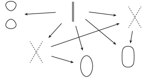
Figure 4. The spaces $D^{2}(f)$ of some singularities adjacent to $B_{\infty}$. Dashed lines correspond to phenomena which are not visible over the reals.

Take the map $f_{t/10,-t,t}$ on the top-left corner of the figure. Its double point space has two connected components $C_{1}$ and $C_{2}$, each containing a $1$-cycle. Each of these components is the image of the other by the generator $\sigma\in S_{2}$. Consequently, for any point $a\in C_{1}$ and any $1$-cycle generating $H_{1}(C_{1})$, the cycles $a,\sigma a$ and $c,\sigma c$ generate $H_{0}(D^{2})$ and $H_{1}(D^{2})$, respectively. It follows that $H_{0}^{\operatorname{Alt}}(D^{2})$ and $H_{1}^{\operatorname{Alt}}(D^{2})$ are generated, respectively, by the non-zero cycles $a-\sigma a$ and $c-\sigma c$. Hence $A_{0}\cong\mathbb{Q}$ and $A_{1}\cong\mathbb{Q}$ are responsible for the homology in dimensions one and two we observed.

Now look at the double spaces of the other maps. Since they are connected, their homology in dimension 0 is generated by any point, say $a\in D^{2}$. Since $a$ and $\sigma a$ are contained in the same connected component, they represent the same homology class. This means that $H_{0}(D^{2})$ is $S_{2}$-invariant, hence $A_{0}=0$ for all these maps.

For 1-dimensional homology, observe that $D^{2}$ is contractible for $B_{1}$ (top-right), while its stable perturbation (bottom-right) contains a 1-dimensional cycle that switches orientation with the action of $S_{2}$. This cycle is the generator of $A_{1}=H_{1}^{\operatorname{Alt}}(D^{2})$ for the mentioned stabilization. Similar considerations can be made for the remaining singularities in the example. Recall that the difference between the two stable perturbations relies on the choice of good representatives, not depicted here.

The argument we gave to study $A_{0}=H_{0}^{\operatorname{Alt}}(D^{2}(f_{a,b,c}))$ for the left-top example generalizes immediately to the following result:

Proposition 5.3.

A stable perturbation of a map germ $\mathbb{C}^{n}\to\mathbb{C}^{m}$, with $2\leq n<m$ has non-trivial 1 dimensional homology if and only if $D^{2}$ has at least one connected component not fixed by $S_{2}$.

References

- [1] J.-L. Cisneros Molina and D. Mond, Multiple points of a simplicial map and the image-computing spectral sequence, arXiv:1911.11095 (2019).
- [2] C.G. Gibson, K. Wirthmüller, A.A. du Plessis, and E.J.N. Looijenga, Topological stability of smooth mappings, Lecture Notes in Mathematics, Springer-Verlag, 1976.
- [3] M. Golubitsky and V. Guillemin, Stable mappings and their singularities, Springer, 1986.
- [4] M. Goresky and R. MacPherson, Stratified Morse Theory, Springer Verlag, 1988.
- [5] V.V. Goryunov, Semi-simplicial resolutions and homology of images and discriminants of mappings, Proc. London Math. Soc. (3) 70 (1995), no. 2, 363–385.
- [6] V.V. Goryunov and D. Mond, Vanishing cohomology of singularities of mappings, Compositio Math. 89 (1993), 45–80.
- [7] H. Hamm, Lokale topologische Eigenschaften komplexer Räume, Math. Ann. 191 (1972), 235–252.
- [8] H. Hamm and Lê Dũng Tráng, Un théorème de Zariski du type de Lefschetz, Annales scientifiques de l’ É.N.S. 4 série, tome 6, no 3 (1973), 317–355.
- [9] H. Hironaka, Stratification and flatness, Real and Complex Singularities (P. Holm, ed.), Nordic Summer School/NAVF, 1977, pp. 199–265.
- [10] K. Houston, Local topology of images of finite complex analytic maps, Topology 36 (1997), no. 5, 1007–1121.
- [11] M. Kato and Y. Matsumoto, On the connectivity of the milnor fiber of a holomorphic function at a critical point, Proc. Internat. Conf., Tokyo (1975), 131–136.
- [12] Lê Dũng Tráng, Some remarks on relative monodromy, Proc. Ninth Nordic Summer School/NAVF Sympos. Math., Oslo 1976 (1977), 397–403.
- [13] W. L. Marar and D. Mond, Multiple point schemes for corank maps, J. London Math. Soc. 2 (1989), no. 3, 553–567.
- [14] J. N. Mather, Stability of -mappings. VI: The nice dimensions, Proceedings of Liverpool Singularities-Symposium, I, 1969/70 192 (1971), 207–253.
- [15] J.W. Milnor, Singular points of complex hypersurfaces, Princenton University Press, 1968.
- [16] David Mond, Vanishing cycles for analytic maps, Singularity theory and its applications, Part I (Coventry, 1988/1989), Lecture Notes in Math., vol. 1462, Springer, Berlin, 1991, pp. 221–234. MR 1129035
- [17] by same author, Disentanglements of corank 2 map-germs: Two examples, Singularities and Foliations. Geometry, Topology and Applications (Raimundo Nonato Araújo dos Santos, Aurélio Menegon Neto, David Mond, Marcelo J. Saia, and Jawad Snoussi, eds.), Springer International Publishing, 2018, pp. 229–258.
- [18] J.J. Nuño-Ballesteros and G. Peñafort Sanchis, Multiple point spaces of finite holomorphic maps, The Quarterly Journal of Mathematics 68 (2017), no. 2, 369–390.
- [19] Dirk Siersma, Isolated line singularities, Singularities, Part 2 (Arcata, Calif., 1981), Proc. Sympos. Pure Math., vol. 40, Amer. Math. Soc., Providence, RI, 1983, pp. 485–496. MR 713274
- [20] R. Thom, Ensemble et morphisme stratifiés, Bulletin of the American Mathematical Society 75 (1969), 240–284.
- [21] H. Whitney, Tangents to an analytic variety, Annals of Mathematics 81, no. 3 (1965), 496–549.
- [22] M. Zach, Topology of isolated determinantal singularities, Ph.D. thesis, Leibniz Universität Hannover, 2017.