A $\phi$-Competitive Algorithm for Scheduling Packets with Deadlines

Abstract

In the online packet scheduling problem with deadlines (PacketSchD, for short), the goal is to schedule transmissions of packets that arrive over time in a network switch and need to be sent across a link. Each packet has a deadline, representing its urgency, and a non-negative weight, that represents its priority. Only one packet can be transmitted in any time slot, so if the system is overloaded, some packets will inevitably miss their deadlines and be dropped. In this scenario, the natural objective is to compute a transmission schedule that maximizes the total weight of packets that are successfully transmitted. The problem is inherently online, with the scheduling decisions made without the knowledge of future packet arrivals. The central problem concerning PacketSchD, that has been a subject of intensive study since 2001, is to determine the optimal competitive ratio of online algorithms, namely the worst-case ratio between the optimum total weight of a schedule (computed by an offline algorithm) and the weight of a schedule computed by a (deterministic) online algorithm.

We solve this open problem by presenting a $\phi$-competitive online algorithm for PacketSchD (where $\phi\approx 1.618$ is the golden ratio), matching the previously established lower bound.

1 Introduction

In the online packet scheduling problem with deadlines (abbreviated PacketSchD), the goal is to schedule transmissions of packets that arrive over time in a network switch and need to be sent across a link. The switch stores incoming packets in a buffer that is assumed to have unlimited capacity. Besides its release time $r_{p}$, each arriving packet $p$ has two other attributes: a deadline $d_{p}$, which is the last time slot when $p$ can be transmitted, and a non-negative weight $w_{p}$. The deadline of $p$ represents its urgency, while its weight represents its importance or priority. (These priorities can be used to implement various levels of service in networks with QoS guarantees.) Only one packet can be transmitted in any time slot, so if the system is overloaded, some packets will inevitably miss their deadlines and be dropped. In this scenario, the natural objective is to compute a transmission schedule that maximizes the total weight of packets that are successfully transmitted. In the literature, this problem is also occasionally referred to as bounded-delay buffer management, QoS buffering, or as a job scheduling problem for unit-length jobs with release times, deadlines, and weights, where the objective is to maximize the weighted throughput. In the offline setting, where the information about all packets is available in advance, it is easy to find an optimal schedule by representing the set of packets as a bipartite graph, with each packet $p$ connected to all slots in its interval $[r_{p},d_{p}]$ by an edge of weight $w_{p}$, and applying any algorithm for the maximum-weight bipartite matching to this graph.

In practice, however, scheduling of packets must be accomplished online, with the scheduling decisions made without the knowledge of future packet arrivals. The central problem concerning PacketSchD, that has been a subject of intensive study since 2001, is to determine the optimal competitive ratio of online algorithms, namely the worst-case ratio between the optimum total weight of a schedule (computed by an offline algorithm) and the weight of a schedule computed by a (deterministic) online algorithm.

This paper provides the solution of this open problem by establishing an upper bound of $\phi$ on the competitive ratio for PacketSchD (where $\phi=(1+\sqrt{5})/2\approx 1.618$ is the golden ratio), matching the previously known lower bound [16, 3, 24, 10]. Our $\phi$-competitive algorithm PlanM is presented in Section 4. The basic idea underlying our algorithm is relatively simple. It is based on the concept of the optimal plan, which, at any given time $t$, is the maximum-weight subset of pending packets that can be feasibly scheduled in the future (if no other packets arrive); we describe it in Section 3. When some packet $p$ from the plan is chosen to be transmitted at time $t$, it will be replaced in the plan by some other packet $\varrho$. The algorithm chooses $p$ to maximize an appropriate linear combination of $w_{p}$ and $w_{\varrho}$. Furthermore, the algorithm makes additional changes in the plan, adjusting deadlines and weights of some packets. These changes are necessary to achieve the competitive ratio $\phi$ and can be viewed as a subtle way to remember necessary information about the past. While the algorithm itself is not complicated, its competitive analysis, given in Section 5, is quite intricate. It relies on showing a bound on amortized profit at each step, using a potential function, which quantifies the advantage of the algorithm over the adversary in future steps, and on maintaining an invariant that allows us to control decreases of the potential function. The ideas leading to the development of algorithm PlanM and its analysis are also outlined in SIGACT News Online Algorithms Column [21].

Past work. The PacketSchD problem was first introduced independently by Hajek [16] and Kesselman et al. [18], who both gave a proof that the greedy algorithm (that always transmits the heaviest packet) is $2$-competitive. Hajek’s paper also contains a proof of a lower bound of $\phi\approx 1.618$ on the competitive ratio. The same lower bound was later discovered independently by Andelman et al. [3, 24] and also by Chin et al. [10] in a different, but equivalent setting. Improving over the greedy algorithm, Chrobak et al. [11, 12] gave an online algorithm with competitive ratio $1.939$. This ratio was subsequently improved to $1.854$ by Li et al. [20], and to $1.828$ by Englert and Westermann [14]. This value of $1.828$, prior to our work, has remained the best upper bound on the competitive ratio of PacketSchD in the published literature.

Algorithms with ratio $\phi$ have been developed for several restricted variants of PacketSchD. Li et al. [19] (see also [17]) gave a $\phi$-competitive algorithm for the case of agreeable deadlines, which consists of instances where the deadline ordering is the same as the ordering of release times, i.e., $r_{p}<r_{q}$ implies $d_{p}\leq d_{q}$ for any packets $p$ and $q$. Another well-studied case is that of $s$-bounded instances, where each packet can be scheduled in at most $s$ slots, that is $d_{p}\leq r_{p}+s-1$ for each packet $p$. A $\phi$-competitive algorithm for $2$-bounded instances was given by Kesselman et al. [18]. This bound was later extended to $3$-bounded instances by Chin et al. [9] and to $4$-bounded instances by Böhm et al. [8]. The work of Bienkowski et al. [6] provides an upper bound of $\phi$ (in a somewhat more general setting) for the case where packet weights increase with respect to deadlines. All these results are tight, as the proof of the lower bound of $\phi$ in [16, 3, 24, 10] is based on an adversary strategy that uses only $2$-bounded instances with increasing weights, and $2$-bounded instances have the agreeable-deadline property.

In $s$-uniform instances, each packet has exactly $s$ consecutive slots where it can be scheduled. (Obviously, such instances also satisfy the agreeable deadlines property.) The lower bound of $\phi$ in [16, 3, 24, 10] does not apply to $s$-uniform instances; in fact, as shown by Chrobak et al. [12], for $2$-uniform instances, competitive ratio $\approx 1.377$ is optimal.

Randomized online algorithms for PacketSchD have been studied as well, although the gap between the upper and lower bounds for the competitive ratio in the randomized case remains quite large. The best upper bound is $\approx 1.582$ [4, 9, 7, 25], and it applies even to the adaptive adversary model. For the adaptive adversary, the best lower bound is $\approx 1.33$ [7], while for the oblivious adversary it is $1.25$ [10].

Kesselman et al. [18] originally proposed the problem in the setting with integer bandwidth $m\geq 1$, which means that $m$ packets are sent in each step. For an arbitrary $m$, they proved that the greedy algorithm is $2$-competitive and that there is a $\phi$-competitive algorithm for $2$-bounded instances [18]. Later, Chin et al. [9] gave an algorithm with ratio that tends to $\frac{e}{e-1}\approx 1.582$ for $m\rightarrow\infty$. The best lower bound for any $m$, also due to Chin et al. [9], equals $1.25$ and holds even for randomized algorithms against the oblivious adversary. Observe that any upper bound for bandwidth $1$ implies the same upper bound for an arbitrary $m$, by simulating an online algorithm for bandwidth $1$ on an instance where each step is subdivided into $m$ smaller steps. Hence, our algorithm in Section 4 is $\phi$-competitive for any $m$, which improves the current state-of-the-art for any $m<13$.

There is a variety of other packet scheduling problems related to PacketSchD. The semi-online setting with lookahead was proposed in [8]. A relaxed variant of PacketSchD in which only the ordering of deadlines is known but not their exact values, was studied in [5], where a lower bound higher than $\phi$ was shown. In the FIFO model (see, for example, [2, 18]), packets do not have deadlines, but the switch has a buffer that can only hold a bounded number of packets, and packets must be transmitted in the first-in-first-out order. More information about PacketSchD and related scheduling problems can be found in a survey paper by Goldwasser [15].

2 Preliminaries

This section provides a formal definition of the PacketSchD problem, along with some useful assumptions used throughout the paper.

The online PacketSchD problem. The instance of PacketSchD is specified by a set of packets, with each packet $p$ represented by a triple $(r_{p},d_{p},w_{p})$, where integers $r_{p}$ and $d_{p}\geq r_{p}$ denote the release time and deadline (or expiration time) of $p$, and $w_{p}\geq 0$ is the weight of $p$. (To avoid double indexing, we sometimes use notation $w(p)$ to denote $w_{p}$ and $d(p)$ for $d_{p}$.) The time is discrete, with time units represented by consecutive integers that we refer to as time slots or steps. In a feasible transmission schedule, a subset of packets is transmitted. Only one packet can be transmitted in each time step, and each packet $p$ can only be transmitted in a slot from the interval $[r_{p},d_{p}]$. (Note that this interval includes slot $d_{p}$.) The objective is to compute a schedule whose total weight of transmitted packets (also called its profit) is maximized.

In the online variant of PacketSchD, which is the focus of our work, the algorithm needs to compute the solution incrementally over time. At any time step $t$, packets with release times equal to $t$ are revealed and added to the set of pending packets (that is, those that are already released, but not yet expired or transmitted). Then the algorithm needs to choose one pending packet to transmit in slot $t$. As this decision is made without the knowledge of packets to be released in future time steps, such an online algorithm cannot, in general, be guaranteed to compute an optimal solution. The quality of the schedules it computes can be quantified using competitive analysis. We say that an online algorithm is $c$-competitive if, for each instance, the optimal profit (computed offline) is at most $c$ times the profit of the schedule computed by the online algorithm.

Useful assumptions. The range of integers used as release times and deadlines is not important, as the whole instance can be shifted in time without affecting the competitive ratio. However, for the sake of concreteness we can assume that the whole instance fits in the interval $[0,{T}]$, where ${T}$ is some large time horizon, and that the first step of the computation takes place at time $0$. Throughout the paper, all time slots are tacitly assumed to be from this finite range. (For notational reasons, we will occasionally also use slot $-1$.)

Without loss of generality, we make two simplifying assumptions:

1. We assume that at each step $t$ and for each $\tau\in[t,{T}]$, there is a pending packet with deadline $\tau$ (or more such packets, if needed). This can be achieved by releasing, at time $t$, virtual $0$-weight packets with deadline $\tau$, for each $\tau\in[t,{T}]$.

2. We also assume that all packets have different weights. Any instance can be transformed into an instance with distinct weights through infinitesimal perturbation of the weights, without affecting the competitive ratio. Thus the virtual packets from the previous assumption have, in fact, infinitesimal positive weights, although in the calculations we treat these values as being equal $0$. The only purpose of this assumption is to facilitate consistent tie-breaking, in particular uniqueness of plans (to be defined shortly).

A careful reader may notice that assumption (A1) as written reveals the value of ${T}$ to the online algorithm. This does not affect our analysis because, for any instance, if the maximum packet deadline in this instance is $d_{{\mbox{\tiny\rm max}}}$, then the computation of our algorithm is independent of the choice of the time horizon ${T}\geq d_{{\mbox{\tiny\rm max}}}$, provided that the ties between weights of virtual $0$-weight packets are broken in favor of earlier-deadline packets, in the sense that those with larger deadlines are considered “lighter”.

The golden ratio. The competitive ratio of our algorithm is $\phi={\textstyle\frac{1}{2}}(\sqrt{5}+1)\approx 1.618$, the famous number known as the golden ratio. Its most important property is that it satisfies the equation $\phi^{2}=\phi+1$. This identity will be frequently used in calculations, usually in the form $\frac{1}{\phi^{2}}+\frac{1}{\phi}=1$. Another useful property is that $\sum_{i=0}^{\infty}\phi^{-2i}=\phi$, which follows easily from the formula for summing a geometric sequence and the earlier-mentioned properties of $\phi$.

3 Plans and their Properties

Consider an execution of some online algorithm. At any time $t$, the algorithm will have a set of pending packets. We now discuss properties of these pending packets and introduce the concept of plans that will play a crucial role in our algorithm.

The set of packets pending at a time $t$ has a natural ordering, called the canonical ordering and denoted $\prec$, which orders packets in non-decreasing order of deadlines, breaking ties in favor of heavier packets. (By assumption (A2) the weights are distinct.) Formally, for two pending packets $p$ and $q$, define $p\prec q$ iff $d_{p}<d_{q}$ or $d_{p}=d_{q}$ and $w_{p}>w_{q}$. The earliest-deadline packet in some subset $X$ of pending packets is the packet that is first in the canonical ordering of $X$. Similarly, the latest-deadline packet in $X$ is the last packet in the canonical ordering of $X$.

Plans. Consider a set $X$ of packets pending at a time step $t$. $X$ is called a plan if the packets in $X$ can be feasibly scheduled in future time slots $t,t+1,...$, where “feasibly” means that all packets in $X$ meet their deadlines. We will typically use symbols ${P},{Q},...$ to denote plans. We emphasize that in a plan we do not assign packets to time slots; that is, a plan is not a schedule. A plan has at least one schedule, but in general it may have many. (In the literature, such scheduled plans are sometimes called provisional schedules.) Using a standard exchange argument, if ${P}$ is a plan then any schedule of ${P}$ can be converted into its canonical schedule, in which the packets from ${P}$ are assigned to the slots $t,t+1,...$ in the canonical order.

For any two time slots $\sigma\geq\tau\geq t$, by $X[\tau,\sigma]={\left\{j\in X{\;:\;}d_{j}\in[\tau,\sigma]\right\}}$ we denote the subset of $X$ consisting of packets whose deadlines are in $[\tau,\sigma]$. In particular, $X[t,\tau]$ contains packets with deadlines at most $\tau$. In a similar way, we define $X[\tau,\sigma)$, $X(\tau,\sigma]$, and $X(\tau,\sigma)$. We also define

$${\textsf{pslack}}(X,\tau)=(\tau-t+1)-|X[t,\tau]|.$$

Note that $\tau-t+1$ is the number of slots in interval $[t,\tau]$. For convenience, we also allow $\tau=t-1$, in which case the above formula gives us that ${\textsf{pslack}}(X,t-1)=0$. We stress that the formula for ${\textsf{pslack}}(X,\tau)$ also depends on the value of $t$. This $t$ will always be the “current step” under consideration and it will be uniquely determined from context, so we do not include it as a parameter of this function, to reduce clutter.

The values of ${\textsf{pslack}}(X,\tau)$ are useful for determining feasibility of $X$:

Observation 3.1.

Let $X$ be a subset of packets pending at some step $t$. $X$ is a plan if and only if ${\textsf{pslack}}(X,\tau)\geq 0$ for each $\tau\geq t$.

This observation is quite straightforward: If $X$ is a plan then, in any (feasible) schedule of $X$, for each $\tau\geq t$ all packets in $X[t,\tau]$ are scheduled in different slots of the interval $[t,\tau]$; thus $|X[t,\tau]|\leq\tau-t+1$. This shows the necessity of the condition in the observation. To show sufficiency, assume that ${\textsf{pslack}}(X,\tau)\geq 0$ for each $\tau\geq t$. This implies, by simple induction, that assigning the packets in $X$ to slots $t,t+1,...$ in the canonical order will produce a schedule (the canonical schedule of $X$, in fact) in which all packets will meet their deadlines.

Throughout the paper, we will tacitly assume that any plan $P$ we consider is full, in the sense that it contains enough packets to fill all slots between the current time $t$ and the time horizon ${T}$; that is $|P[t,{T}]|={T}-t+1$. This assumption can be made without loss of generality because there are always sufficiently many infinitesimal-weight packets pending, by Assumption (A1). With this assumption, the concepts of tight slots, segments, etc., to be introduced below will be always well defined.

Let ${P}$ be a plan for the set of packets pending at some time $t$. We now discuss the structure of ${P}$. (See Figure 3.1 for an illustration.) Slot $\tau\geq t$ is called tight in ${P}$ if ${\textsf{pslack}}({P},\tau)=0$. In particular, according to our conventions above, slots $t-1$ and $T$ are tight. If the tight slots of ${P}$ are $t_{0}=t-1<t_{1}<t_{2}<\cdots<t_{c}=T$, then for each $i=1,2,...,c$ the time interval $(t_{i-1},t_{i}]={\left\{t_{i-1}+1,t_{i-1}+2,\dots,t_{i}\right\}}$ is called a segment of ${P}$. In other words, the tight slots divide the time range into segments, each starting right after a tight slot and ending at (and including) the next tight slot. The significance of a segment $(t_{i-1},t_{i}]$ is that in any schedule of ${P}$ all packets in ${P}(t_{i-1},t_{i}]$ must be scheduled in this segment. Thus, slightly abusing terminology, we occasionally think of each segment as a set of packets to be scheduled in this segment, namely the set ${P}(t_{i-1},t_{i}]$. Within a segment, packets from ${P}$ can be permuted, although only in some restricted ways. In particular, the first slot of a segment may contain any packet from that segment (see Observation A.1). Let $\alpha=t_{1}$ be the first tight slot of plan ${P}$ (we regard tight slot $t_{0}=t-1$ as the “0-th tight slot”). The first tight slot $\alpha$ will play a special role in our algorithm, together with the segment $[t,\alpha]=(t_{0},t_{1}]$ of ${P}$, called the initial segment. Whenever we consider several plans at a time $t$ and some ambiguity arises, we will write $\alpha=\alpha_{{P}}$, to indicate that $\alpha$ is the first tight slot for this specific plan ${P}$.

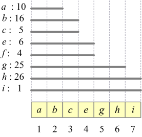
Figure 3.1: An example of an instance with optimal plan ${P}={\left\{a,b,c,e,g,h,i\right\}}$ and its canonical schedule in time slots $1,2,...,7$. Each packet is represented by one row, that shows this packet’s identifier and weight (separated by colon), followed by a line segment stretching from the current time slot $t$ (assumed to be $1$ here) to this packet’s deadline. Note that packet $f$ is not in ${P}$, even though it is heavier than $i$. The segments of ${P}$ are $(0,3]$, $(3,4]$, $(4,7]$. (Alternatively, in terms of packets from ${P}$, these segments are ${\left\{a,b,c\right\}}$, ${\left\{e\right\}}$, ${\left\{g,h,i\right\}}$.) The values of ${\textsf{minwt}}({P},\tau)$ are: $5$ for $\tau\in{\left\{1,2,3,4\right\}}$, and $1$ for $\tau\in{\left\{5,6,7\right\}}$.

For a plan ${P}$ and a slot $\tau\geq t$, let $\textsf{nextts}({P},\tau)$ be the earliest tight slot $\tau^{\prime}\geq\tau$ and let $\textsf{prevts}({P},\tau)$ be the latest tight slot $\tau^{\prime}<\tau$. Both notations are well-defined: that $\textsf{nextts}({P},\tau)$ is well-defined follows from slot $T$ being tight, and $\textsf{prevts}({P},\tau)$ is well-defined because $t-1$ is a tight slot, according to our convention. (Both functions also depend on $t$, but $t$ is implied, since $t$ is the time for which $P$ is defined. This convention will apply to other notations involving plans.)

The notion that will be crucial in the design of our $\phi$-competitive algorithm is the minimum weight of a packet that can appear in a schedule of the plan in some slot between the current time $t$ and a given slot $\tau$. Naturally, the packets that are candidates for this minimum include all packets in segments ending before $\tau$, but also we need to include all packets in the segment of $\tau$, even those with deadlines larger than $\tau$. (This is because, as explained earlier, each packet in a segment can be scheduled at the beginning of that segment.) Formally, for a plan ${P}$ at time $t$ and a slot $\tau\geq t$, define

$${\textsf{minwt}}({P},\tau)=\min{\left\{\,w_{j}{\;:\;}j\in{P}[t,\textsf{nextts}({P},\tau)]\,\right\}}.$$

We will occasionally omit ${P}$ in this notation if it is understood from context. By definition, if we fix $t$ and ${P}$ and think of ${\textsf{minwt}}({P},\tau)$ as a function of $\tau$, then this function is monotonely non-increasing over the whole range of $\tau=t,t+1,...,T$, and is constant in each segment (that is, all slots $\tau$ in any given segment have the same value of ${\textsf{minwt}}({P},\tau)$).

Optimal plans. Given a set of packets ${{\mathcal{U}}}$ pending at a given time $t$, their plan ${P}$ is called optimal if it has the maximum weight among all plans of these packets. Since the collection of such plans forms a matroid (which is easy to verify using Observation 3.1; see also e.g. [18]), the optimal plan at step $t$ can be computed by the following greedy algorithm:

Algorithm 1 Algorithm ${\textsf{ComputePlan}}({{\mathcal{U}}},t)$

1:${{\mathcal{U}}}$ is a set of packets pending at time $t$

2:$X\,{\leftarrow}\,\emptyset$

3:for each packet $j\in{{\mathcal{U}}}$ in order of decreasing weights do

4:     if ${\textsf{pslack}}(X\cup{\left\{j\right\}},\tau)\geq 0$ for all $\tau\geq t$ then

5:         $X\,{\leftarrow}\,X\cup{\left\{j\right\}}$      

6:${P}\,{\leftarrow}\,X$ $\triangleright$ ${P}$ is the optimal plan for ${{\mathcal{U}}}$

Assumption (A2) about different weights implies that the optimal plan ${P}$ computed above is unique. See Figure 3.1 for an example of an optimal plan for a given set of pending packets.

During a computation, the set of pending packets can change. There are two types of events that can cause this change: an arrival of a new packet and a transmission of a packet, which also involves incrementing the current time and dropping all newly expired packets. This will also cause the optimal plan to change. The matroid property implies that at most one packet in the optimal plan changes after each event (not counting the transmitted packet in a transmission event). These changes are fairly intuitive and we outline them briefly below; for a formal description of these changes, correctness proofs, and figures with examples, see Appendix A.

In the discussion below, we assume that $t$ is the current time step and ${P}$ is the current optimal plan, right before an arrival or transmission event. By ${Q}$ we will denote the optimal plan right after the event. For a slot $\tau\geq t$, whenever we refer to the change of ${\textsf{pslack}}(\tau)$ (that it increases, decreases, or remains the same), without specifying the plan, we mean the change from ${\textsf{pslack}}({P},\tau)$ to ${\textsf{pslack}}({Q},\tau)$. We use the same convention for function ${\textsf{minwt}}(\tau)$.

Packet arrivals. We first consider the event of a new packet $s$ arriving at time $t$. As $s$ is added to the set of pending packets, the optimal plan needs to be updated accordingly. Define $f\in{P}$ to be the packet with $w_{f}={\textsf{minwt}}({P},d_{s})$, that is the lightest packet in ${P}$ with $d_{f}\leq\textsf{nextts}({P},d_{s})$. If $w_{s}<w_{f}$, then $s$ is not added to the optimal plan, which thus stays the same. On the other hand, if $w_{s}>w_{f}$ then $s$ is added to the optimal plan and $f$ is forced out, i.e., the new optimal plan is ${Q}={P}\cup\{s\}\setminus\{f\}$. In the latter case, it is interesting to see how the values of ${\textsf{pslack}}(\tau)$ and the segments change:

• If $d_{s}\geq d_{f}$, then ${\textsf{pslack}}({Q},\tau)={\textsf{pslack}}({P},\tau)+1$ for $\tau\in[d_{f},d_{s})$. Therefore, all tight slots in $[d_{f},d_{s})$ in $P$ are no longer tight in $Q$ and the segments containing $d_{f}$ and $d_{s}$ and all segments in-between get merged into one segment of ${Q}$.

• If $d_{s}<d_{f}$, then $d_{f}$ and $d_{s}$ must be in the same segment of ${P}$ (because $d_{f}\leq\textsf{nextts}({P},d_{s})$) and ${\textsf{pslack}}({Q},\tau)={\textsf{pslack}}({P},\tau)-1$ for $\tau\in[d_{s},d_{f})$. Thus, there may be new tight slots in $[d_{s},d_{f})$, resulting in new segments.

In both cases, the values of ${\textsf{pslack}}(\tau)$ remain the same for other slots $\tau\geq t$; thus other tight slots and segments do not change. Moreover, ${\textsf{minwt}}({Q},\tau)\geq{\textsf{minwt}}({P},\tau)$ holds for any slot $\tau\geq t$; this property will play a significant role in our algorithm.

Transmitting a packet. Next, we discuss the changes of the optimal plan resulting from a transmission event. Throughout the paper, only packets in the optimal plan will be considered for transmission. The scenario is this: We consider the set ${{\mathcal{U}}}$ of all packets pending at time $t$, and the optimal plan ${P}$ for ${{\mathcal{U}}}$. We choose some packet $p\in{P}$, transmit it at time $t$, and increment the current time to $t+1$. The new set ${{\mathcal{U}}}^{\prime}$ of pending packets (now at time $t+1$) is obtained from ${{\mathcal{U}}}$ by removing $p$ and all packets with deadline $t$. As before, we will use ${Q}$ to denote the new optimal plan after this change, namely the optimal plan for ${{\mathcal{U}}}^{\prime}$ with respect to time $t+1$.

If $p$ is from the initial segment $[t,\alpha]$ of ${P}$, then ${Q}={P}\setminus{\left\{p\right\}}$. In this case ${\textsf{pslack}}({Q},\tau)={\textsf{pslack}}({P},\tau)-1$ for $\tau\in[t+1,d_{p})$ and ${\textsf{pslack}}(\tau)$ remains unchanged for $t\geq d_{p}$. This implies that new tight slots may appear before $d_{p}$, i.e., the initial segment may get divided into more segments. Furthermore, ${\textsf{minwt}}(\tau)$ does not decrease for any $\tau\geq t+1$.

The more interesting case is when $p$ is from a later segment. Let ${\ell}$ be the lightest packet in ${P}[t,\alpha]$, i.e., in the initial segment, and let $\varrho$ be the heaviest pending packet not in ${P}$ that satisfies $d_{\varrho}>\textsf{prevts}({P},d_{p})$ (such a packet $\varrho$ exists by Assumption (A1)). Using the matroid property of the feasible sets of packets at time $t+1$ and the structure of the plan, in Appendix A we prove that ${Q}={P}\setminus\{p,{\ell}\}\cup\{\varrho\}$. Furthermore, in this case we have:

• ${\textsf{pslack}}({Q},\tau)={\textsf{pslack}}({P},\tau)-1$ for $\tau\in[t+1,d_{\ell})$. There may be new tight slots in the interval $[t+1,d_{\ell})$, resulting in new segments.

• If $d_{\varrho}\geq d_{p}$, then ${\textsf{pslack}}({Q},\tau)={\textsf{pslack}}({P},\tau)+1$ for $\tau\in[d_{p},d_{\varrho})$. Here, all segments that overlap $[d_{p},d_{\varrho}]$ are merged into one segment of ${Q}$.

• If $d_{\varrho}<d_{p}$, then ${\textsf{pslack}}({Q},\tau)={\textsf{pslack}}({P},\tau)-1$ for $\tau\in[d_{\varrho},d_{p})$. (In this case, $d_{p}$ and $d_{\varrho}$ must be in the same segment of ${P}$, because $d_{\varrho}>\textsf{prevts}({P},d_{p})$.) As a result of decreasing some ${\textsf{pslack}}(\tau)$ values, new tight slots may appear in $[d_{\varrho},d_{p})$, creating new segments.

For slots $\tau\geq t+1$ not covered by the cases above, the value of ${\textsf{pslack}}(\tau)$ does not change. Unlike for packet arrivals, after a packet transmission event some values of ${\textsf{minwt}}(\tau)$ may decrease, either due to $\varrho$ being included in ${Q}$ or as a side-effect of segments being merged.

Substitute packets. The aforementioned updates of the plan motivate the following definition: Let ${{\mathcal{U}}}$ be the set of all packets pending at time $t$ and ${P}\subseteq{{\mathcal{U}}}$ be the optimal plan at time $t$. For each $j\in{P}$ we define the substitute packet of $j$, denoted $\textsf{sub}({P},j)$, as follows. If $j\in{P}[t,\alpha]$, then $\textsf{sub}({P},j)={\ell}$, where ${\ell}$ is the lightest packet in ${P}[t,\alpha]$. If $j\notin{P}[t,\alpha]$, then $\textsf{sub}({P},j)$ is the heaviest pending packet $\varrho\in{{\mathcal{U}}}\setminus{P}$ that satisfies $d_{\varrho}>\textsf{prevts}({P},d_{j})$, which exists by assumption (A1).

By definition, all packets in a segment of ${P}$ have the same substitute packet. Also, for any $j\in{P}$ it holds that $w_{j}\geq w(\textsf{sub}({P},j))$. This is because for $j\in{P}[t,\alpha]$ we have $\textsf{sub}({P},j)={\ell}$ and $w_{j}\geq w_{\ell}$ (the equality will hold only when ${\ell}=j$), while for $j\in{P}(\alpha,{T}]$ we have $d(\textsf{sub}({P},j))>\textsf{prevts}({P},d_{j})$; thus in this case the set ${P}-{\left\{j\right\}}\cup{\left\{\textsf{sub}({P},j)\right\}}$ is feasible, and the optimality of ${P}$ implies that $w_{j}>w(\textsf{sub}({P},j))$.

4 Online Algorithm

This section presents our online algorithm PlanM for PacketSchD, starting with some intuitions and additional notation, and followed by two examples where its competitive ratio is exactly $\phi$.

Intuitions. Similar to other online profit maximization problems, the main challenge in achieving a small competitive ratio for PacketSchD is in finding the right balance between the immediate profit and future profits. Let ${P}$ be the optimal plan at a step $t$. Consider the greedy algorithm for PacketSchD, which at time $t$ transmits the heaviest pending packet $h$, which is always in ${P}$. We focus on the case when $h$ is not in the initial segment. (The case when $h$ is in the initial segment is different, but similar intuitions apply to it as well.) In the next step, after transmitting $h$ but before new packets are released, $h$ will be replaced in the optimal plan by its substitute packet $\varrho_{h}=\textsf{sub}(P,h)$. This packet could be very light, possibly $w(\varrho_{h})\approx 0$. Suppose that there is another packet $g$ in ${P}$ with $d_{g}<d_{h}$ and $w_{g}\approx w_{h}$ whose substitute packet $\varrho_{g}=\textsf{sub}(P,g)$ is quite heavy, say $w(\varrho_{g})\approx w_{g}$. Thus, instead of $h$ we can transmit $g$ at time $t$, achieving roughly the same immediate profit as from transmitting $h$, but with essentially no decrease in the weight of the optimal plan (which serves as a rough estimate of future profits). This example indicates that a reasonable strategy would be to choose a packet $p$ based both on its weight and the weight of its substitute packet. Following this intuition, our algorithm chooses $p$ that maximizes $w_{p}+\phi\cdot w(\textsf{sub}(P,p))$, breaking ties arbitrarily. The choice of the coefficients in the objective function follows the intuition from analyzing the $2$-bounded case; see the discussion of examples in Figure 4.2.

As it turns out, the above strategy for choosing $p$ does not, by itself, guarantee $\phi$-competitiveness. The analysis of special cases and an example where this simple approach fails lead to the second idea behind our algorithm (we describe the example in Appendix C). The difficulty is related to how the values of ${\textsf{minwt}}(\tau)$, for a fixed $\tau$, vary while the current time $t$ increases. We were able to show $\phi$-competitiveness of the above strategy for certain instances where ${\textsf{minwt}}(\tau)$ monotonely increases as $t$ grows from $0$ to $\tau$. We call this property slot-monotonicity. To extend slot-monotonicity to instances where it does not hold, the idea is then to simply force it to hold by decreasing deadlines and increasing weights of some packets in the new optimal plan. (To avoid unfairly benefiting the algorithm from these increased weights, we will need to account for them appropriately in the analysis.) From this point on, the algorithm proceeds using these new weights and deadlines when computing the optimal plan and choosing a packet for transmission.

Notation. To avoid ambiguity, we will index various quantities used by the algorithm with the superscript $t$ that represents the current time. This includes weights and deadlines of some packets, since these might change over time.

• We use notations $w^{t}_{j}$ and $d^{t}_{j}$ for the weight and the deadline of a packet $j$ in step $t$, before the transmission of this step is implemented. (Our algorithm only changes weights and deadlines when transmitting a packet, so they are not affected by packet arrivals.) To avoid double subscripts, we occasionally write $w^{t}(j)$ and $d^{t}(j)$ instead of $w^{t}_{j}$ and $d^{t}_{j}$. We will sometimes use notation $w^{0}_{j}$ for the original weight of packet $j$, when notation $w_{j}$ may lead to some ambiguity. We will also omit $t$ in these notations whenever $t$ is unambiguously implied from context.

• ${{{P}}^{t}}$ is the optimal plan at time $t$ after all packets $j$ with $r_{j}=t$ arrive and before a packet is transmitted.

• We write $\textsf{sub}^{t}(p)$ to denote $\textsf{sub}({{{P}}^{t}},p)$ and we adopt similar conventions for ${\textsf{minwt}}^{t}(\tau)$, $\textsf{nextts}^{t}(\tau)$, and $\textsf{prevts}^{t}(\tau)$.

• $\alpha=\textsf{nextts}^{t}(t)$ is the first tight slot of ${{{P}}^{t}}$, so $[t,\alpha]$ is the initial segment.

• ${\ell}$ is the lightest packet in ${{{P}}^{t}}[t,\alpha]$.

• $\varrho$, $h_{i}$, $\gamma$, $\tau_{i}$, and $k$ will refer to the packets and values chosen in Algorithm $\textsf{PlanM}(t)$.

Algorithm 2 Algorithm $\textsf{PlanM}(t)$

1:transmit packet $p\in{{{P}}^{t}}$ that maximizes $w^{t}_{p}+\phi\cdot w^{t}(\textsf{sub}^{t}(p))$

2:if $d^{t}_{p}>\alpha$ then $\triangleright$ “leap step”

3:     $\varrho\,{\leftarrow}\,\textsf{sub}^{t}(p)$

4:     $w^{t+1}_{\varrho}\,{\leftarrow}\,{\textsf{minwt}}^{t}(d^{t}_{\varrho})$ $\triangleright$ increase $w_{\varrho}$

5:     $\gamma\,{\leftarrow}\,\textsf{nextts}^{t}(d^{t}_{\varrho})$ and $\tau_{0}\,{\leftarrow}\,\textsf{nextts}^{t}(d^{t}_{p})$

6:     $i\,{\leftarrow}\,0$ and $h_{0}\,{\leftarrow}\,p$

7:     while $\tau_{i}<\gamma$ do

8:         $i\,{\leftarrow}\,i+1$

9:         $h_{i}\,{\leftarrow}\,$ heaviest packet in ${{{P}}^{t}}(\tau_{i-1},\gamma]$

10:         $\tau_{i}\,{\leftarrow}\,\textsf{nextts}^{t}(d^{t}_{h_{i}})$

11:         $d^{t+1}_{h_{i}}\,{\leftarrow}\,\tau_{i-1}$ and $w^{t+1}_{h_{i}}\,{\leftarrow}\,\max(w^{t}_{h_{i}},{\textsf{minwt}}^{t}(\tau_{i-1}))$ $\triangleright$ adjusting packet $h_{i}$      

12:     $k\,{\leftarrow}\,i$ $\triangleright$ final value of $i$

The pseudo-code of our algorithm, called $\textsf{PlanM}(t)$, is given in Algorithm 2. For a pending packet $j$, if $w^{t+1}_{j}$ (resp. $d^{t+1}_{j}$) is not explicitly set in the algorithm, then its value remains the same by default, that is $w^{t+1}_{j}\,{\leftarrow}\,w^{t}_{j}$ (resp. $d^{t+1}_{j}\,{\leftarrow}\,d^{t}_{j}$).

Let $p$ be the packet sent by PlanM in step $t$. If $p$ is in the initial segment $[t,\alpha]$ of ${{{P}}^{t}}$, the step is called an ordinary step. Otherwise (if $d^{t}_{p}>\alpha$), the step is called a leap step, and then $\varrho=\textsf{sub}^{t}(p)$ is the heaviest pending packet $\varrho\not\in{{{P}}^{t}}$ with $d^{t}_{\varrho}>\textsf{prevts}^{t}(d^{t}_{p})$. We will further consider two types of leap steps. If $d_{p}$ and $d_{\varrho}$ are in the same segment, then this step is called a simple leap step; in that case $\gamma=\tau_{0}$, the while loop is not executed, and $k=0$. If $d_{\varrho}$ is in a later segment than $d_{p}$, then this step is called an iterated leap step; in that case $\gamma>\tau_{0}$, the while loop is executed at least once, and $k>0$.

As all packets in the segment of ${{{P}}^{t}}$ that contains $p$ have the same substitute packet $\textsf{sub}^{t}(p)$, $p$ must be the heaviest packet in its segment. Furthermore, $p$ is not too light compared to the heaviest pending packet $h$; specifically, we have that $w_{p}\geq w_{h}/\phi^{2}$. Indeed, as mentioned earlier, we have $w_{p}\geq w(\textsf{sub}^{t}(p))$. It follows that $\phi^{2}w_{p}=w_{p}+\phi w_{p}\geq w_{p}+\phi\cdot w(\textsf{sub}^{t}(p))\geq w_{h}+\phi\cdot w(\textsf{sub}^{t}(h))\geq w_{h}$, where the second inequality follows by the choice of $p$ in line 1 of Algorithm $\textsf{PlanM}(t)$.

Slot-monotonicity. Our goal is to maintain the slot-monotonicity property, i.e., to ensure that for any fixed slot $\tau$ the value of ${\textsf{minwt}}^{t}(\tau)$ does not decrease as the current time $t$ progresses from $0$ to $\tau$. For this reason, we need to increase the weight of the substitute packet $\varrho$ in each leap step (as $w^{t}_{\varrho}<{\textsf{minwt}}^{t}(d^{t}_{\varrho})$), which is done in line 4. (To maintain Assumption (A2), we add an infinitesimal to the new weight of $\varrho$.) For the same reason, in the iterated leap step, we also need to adjust the deadlines and weights of the packets $h_{i}$, which is done in line 11. The deadlines of $h_{i}$’s are decreased to make sure that the segments between $\beta=\textsf{prevts}^{t}(d^{t}_{p})$ and $\gamma$ do not merge (as merging could cause a decrease of some values of ${\textsf{minwt}}^{t}(\tau)$). These deadline changes can be thought of as a sequence of substitutions, where $h_{1}$ replaces $p$ in the segment of ${P}$ ending at $\tau_{0}$, $h_{2}$ replaces $h_{1}$, etc., and finally, $\varrho$ replaces $h_{k}$ in the segment ending at $\gamma$. We sometimes refer to this process as a “shift” of the $h_{i}$’s. See Figure 4.1 for an illustration. Then, if the weight of some $h_{i}$ is too low for its new segment, it is increased to match the earlier minimum of that segment, that is ${\textsf{minwt}}^{t}(\tau_{i-1})$. (Again, to maintain Assumption (A2), we add an infinitesimal to the new weight of $h_{i}$.)

In ordinary steps, the algorithm does not make any weight and deadline changes. Thus, in such steps the optimal plan changes as described earlier in Section 3 and the slot monotonicity property is preserved. (See Appendix A for formal proofs.)

In leap steps, the algorithm modifies weights and deadlines of some packets, and thus the discussion from Section 3 does not apply directly. The changes in the optimal plan after a leap step are elaborated in detail in Lemma B.1 in Appendix B. We briefly summarize them here. Recall that in a leap step the packet $p$ is in some non-initial segment. Let ${P}={{{P}}^{t}}$ and let ${Q}$ be the optimal plan after $p$ is transmitted, the time is incremented to $t+1$, and weights and deadlines are changed (according to lines 3-11 in the algorithm). Let also ${\overline{{Q}}}$ be the intermediate optimal plan after $p$ is transmitted and the time is incremented, but before the algorithm adjusts weights and deadlines. As discussed in Section 3, this plan is ${\overline{{Q}}}={P}\setminus{\left\{p,{\ell}\right\}}\cup{\left\{\varrho\right\}}$, where $\varrho=\textsf{sub}^{t}(p)$.

In a simple leap step, only the weight of $\varrho$ is modified. Increasing the weight of a packet in the optimal plan does not affect its optimality and thus ${Q}={\overline{{Q}}}$. Furthermore, no segments are merged, i.e., any tight slot of ${P}$ is tight in ${Q}$ as well.

In an iterated leap step, by the choice of $p$, the definition of $h_{i}$’s in line 9, and the while loop condition in line 7, we have that $w^{t}_{p}=w^{t}_{h_{0}}>w^{t}_{h_{1}}>w^{t}_{h_{2}}>\cdots>w^{t}_{h_{k}}>w^{t}_{\varrho}$ and that $h_{k}$ is in the segment of ${P}$ ending at $\gamma$, that is $\textsf{prevts}^{t}(d^{t}_{\varrho})<d^{t}_{h_{k}}\leq\gamma$. As in the simple leap step, increasing the weight of a packet does not affect the optimality of a plan. Moreover, a careful analysis of the changes of ${\textsf{pslack}}()$ values yields that decreasing the deadlines of $h_{1},h_{2},\ldots,h_{k}$ (in line 11) does not change the optimal plan, so we can conclude that ${Q}={\overline{{Q}}}$ holds in an iterated leap step as well. The decrease of the deadlines of $h_{i}$’s also ensures that no segments are merged. (See Appendix B for complete proofs.)

The property that no segments are merged, together with the increase of the weights, allows us to prove that ${\textsf{minwt}}^{t}(\tau)$ does not decrease for any $\tau$ even in a leap step. This slot monotonicity property is summarized in the lemma below, whose proof follows directly from Lemma A.2(c), Lemma A.4(c), and Lemma B.2.

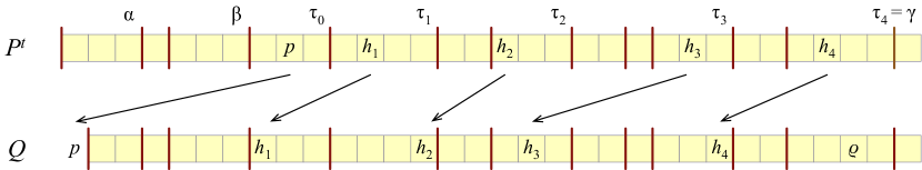
Figure 4.1: An illustration of the shift of packets $h_{1},\dots,h_{k}$ (for $k=4$) in lines 6-11 in an iterated leap step. In this figure, $\beta=\textsf{prevts}^{t}(d^{t}_{p})$ and ${Q}$ is the plan right after $p$ is transmitted and the current time is incremented to $t+1$ (but before packets released at time $t+1$ are taken into account). Both plans are represented by their canonical schedules. Vertical dark-red lines separate the segments of the plans.

Lemma 4.1.

Let ${P}$ be the current optimal plan in step $t$ just before an event of either arrival of a new packet or transmitting a packet (and incrementing the current time), and let ${Q}$ be the plan after the event. Then ${\textsf{minwt}}({Q},\tau)\geq{\textsf{minwt}}({P},\tau)$ for any $\tau>t$, and also for $\tau=t$ in case of a packet arrival. Hence, in the computation of Algorithm PlanM, for any fixed $\tau$, the function ${\textsf{minwt}}^{t}(\tau)$ is non-decreasing in $t\in[0,\tau]$.

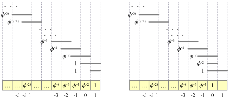
Figure 4.2: Two examples where the competitive ratio of Algorithm PlanM is $\phi$. Packets are identified by their weight. We show the schedules of PlanM at the bottom and time slot indices below the schedules.

Tight examples. To illustrate the computation of Algorithm PlanM, we now give two examples of 2-bounded instances where the competitive ratio is exactly $\phi$. They also give some intuition for the choice of coefficients in line 1 of Algorithm PlanM, as the chosen coefficients exactly balance the competitive ratio for these two examples. We note that, interestingly, there is another combination of the coefficients that gives ratio $\phi$ for the $2$-bounded case, namely $\phi\cdot w_{p}+w(\textsf{sub}(P,p))$; we do not know if these coefficients can yield an optimal algorithm for the general case.

Before we examine these examples, consider the instance where we have two packets pending at some step $t$, one tight packet $q$ with $d_{q}=t$ and $w_{q}=c$, and one packet $r$ with $d_{r}=t+1$ and $w_{r}=\phi^{2}c$. The optimal plan is ${P}^{t}={\left\{q,r\right\}}$ and $\alpha=t$. In this case we have a tie in line 1 of Algorithm PlanM: For $p=q$ the substitute packet is $\ell=q$ and the objective value is $w_{q}+\phi{\,}w_{q}=\phi^{2}{\,}c$, and for $p=r$ the substitute packet has weight $0$ and the objective value is $w_{r}+\phi{\,}0=\phi^{2}{\,}c$ as well. In the examples below, we will assume that we can break this tie either way. This can be accomplished by infinitesimally perturbing the weights, without affecting the competitive ratio.

The two examples are shown in Figure 4.2. For simplicity, in these examples packets are identified by their weight and we allow negative-valued time steps. In both examples, the instance involves a sequence of packets, where at time $-i$, for $i\geq 0$, a packet of weight $\phi^{-2i}$ and deadline $-i+1$ is released. For simplicity, we will think of this sequence as starting at $-\infty$.

In the instance on the left, we have one additional tight packet of weight $1$ released at time $1$. In this instance we break the ties so that the algorithm schedules each packet $\phi^{-2i}$ at time $-i+1$ (thus, at each step $-i\leq 0$, we transmit the tight pending packet). As a result, the algorithm will be able to transmit only one packet of weight $1$, and its profit will be $\sum_{i=0}^{\infty}\phi^{-2i}=1/(1-\phi^{-2})=\phi$. The optimum solution schedules all packets, so its profit is $1+\sum_{i=0}^{\infty}\phi^{-2i}=\phi^{2}$.

In the instance on the right, we have one additional tight packet of weight $\phi^{-2}$ released at time $0$. Here, we also break the ties in favor of the tight pending packet until time $-1$, but at time $0$ the algorithm transmits the packet of weight $1$. The algorithm’s profit will be $\sum_{i=0}^{\infty}\phi^{-2i}-\phi^{-2}=\phi-\phi^{-2}=1+\phi^{-1}-\phi^{-2}=2/\phi$. The optimum solution schedules all packets, so its profit is $\sum_{i=0}^{\infty}\phi^{-2i}+\phi^{-2}=2$.

Comparison to previous algorithms. Our algorithm shares some broad features with known algorithms in the literature. In fact, any online algorithm (with competitive ratio below $2$) needs to capture the tradeoff between weight and urgency when transmitting a packet, so some similarities between these algorithms are inevitable. As we found in our earlier attempts, however, the exact mechanism of formalizing this tradeoff is critical, and minor tweaks can dramatically affect the competitive ratio.

Some prior algorithms used the notion of the optimal provisional schedule, which coincides with our concept of canonically ordered optimal plan; recall that in our paper a plan is defined as a feasible set of pending packets rather than their particular schedule. For example, the $\phi$-competitive algorithm MG for instances with agreeable deadlines by Li et al. [19] (see also [17]) transmits packets from the optimal plan only, either the heaviest packet $h$ or the earliest-deadline packet $e$. (Strictly speaking, this is true for the simplified variant of MG [17], whereas the original version of MG transmitted either $e$ or another sufficiently heavy packet from the optimal plan [19].) The same authors [20] later designed a modified algorithm called DP that achieves competitive ratio $3/\phi\approx 1.854$ for arbitrary instances.

Our approach is more similar to that of Englert and Westermann [14], who designed a $1.893$-competitive memoryless algorithm and an improved $1.828$-competitive variant with memory. Both their algorithms are based on the notion of suppressed packet supp(${P},p$), for a packet $p$ in the plan ${P}$, which, in our terminology, is the same as the substitute packet $\textsf{sub}({P},p)$ if $p$ is not in the initial segment. However, the two concepts differ for packets $p$ in the initial segment. The memoryless algorithm in [14] identifies a packet $m$ of maximum “benefit”, which is measured by an appropriate linear combination of $w_{m}$ and $w(\textsf{supp}({P},m))$, and sends either $m$ or $e$ (the earliest-deadline packet in the optimal plan), based on the relation between $w_{e}$ and the benefit of $m$. The algorithm with memory in [14] extends this approach by comparing $m$’s benefit to $e$’s “boosted weight” $\max(w_{e},\delta(t))$, where $t$ is the current step and $\delta(\tau)$ is the maximum value of ${\textsf{minwt}}({P}^{t^{\prime}},\tau)$ over $t^{\prime}<t$. We remark that considering this value of $\delta(\tau)$ takes into account the previous maximal value of ${\textsf{minwt}}(\tau)$, however, it does not prevent actual decreases of ${\textsf{minwt}}(\tau)$.

Our algorithm involves several new ingredients that are critical to establishing the competitive ratio of $\phi$. First, our analysis relies on full characterization of the evolution of the optimal plan over time, in response to packet arrivals and transmission events. This characterization is sketched in Section 3 and formally treated in Appendix A. Second, we introduce a new objective function $w^{t}_{p}+\phi\cdot w^{t}(\textsf{sub}^{t}(p))$ for selecting a packet $p$ for transmission. This function is based on a definition of substitute packets, $\textsf{sub}({P},p)$, that accurately reflects the changes in the optimal plan following transmission events, including the case when $p$ is in the initial segment. Third, we introduce the concept of slot monotonicity, and devise a way for the algorithm to maintain it over time, using adjustments of weights and deadlines of the packets in the optimal plan. This property is very helpful in keeping track of the optimal profit. Last but not least, we develop several tools used in the amortized analysis of Algorithm $\textsf{PlanM}(t)$, including the concepts of a backup plan, an adversary’s stash, and a novel potential function that captures the relative “advantage” of the algorithm over the adversary in terms of procuring future profits.

5 Competitive Analysis

Let ALG be the schedule computed by PlanM for the instance of PacketSchD under consideration, and let OPT be a fixed optimal schedule for this instance. (Actually, OPT can be any schedule for this instance.) For any time step $t$, by ${\textsf{ALG}}[t]$ and ${\textsf{OPT}}[t]$ we will denote packets scheduled by ALG and OPT, respectively, in slot $t$. (By assumption (A1), we can assume that ${\textsf{ALG}}[t]$ and ${\textsf{OPT}}[t]$ are defined for all steps $t$.) Our overall goal is to show that $\phi\cdot w^{0}({\textsf{ALG}})\geq w^{0}({\textsf{OPT}})$, where, as defined earlier, we use notation $w^{0}_{j}$ for the original weight of packet $j$.

Notational convention. The optimal plan changes in the course of the algorithm’s run, as a result of new packets arriving or of packets being transmitted. In some contexts, it is convenient to think of the current optimal plan as a dynamic set, which we will denote by ${{\mathcal{P}}}$. When more formal treatment is needed, we will use letters ${P},{Q},\dots$, often with appropriate subscripts or superscripts, to denote the “snapshot”, i.e., the current contents, of the optimal plan before or after a particular change. Namely, as already defined in Section 4, ${{{P}}^{t}}$ is the snapshot of the optimal plan after all packets arrive and before a packet is transmitted in step $t$. Furthermore, by ${\widetilde{{P}}^{t}}$ we denote the optimal plan before any packet arrives in step $t$. Thus, as a result of transmitting a packet in step $t$, the optimal plan changes from ${{{P}}^{t}}$ to ${\widetilde{{P}}^{t+1}}$. (See Figure 5.1.) We define more snapshots in the analysis of a transmission event, which will be split into more substeps. For clarity, the superscript of a particular snapshot contains the time index with respect to which the optimal plan is computed (unless it is clear from the context).

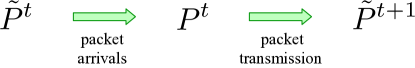
Figure 5.1: Notation for snapshots of the optimal plan ${{\mathcal{P}}}$.

The same conventions apply to other subsets of pending packets used in the analysis: ${{\mathcal{A}}}$ and ${{\mathcal{B}}}$, which we will define shortly. In general, we think of such sets of packets as dynamic sets that change over time as new packets arrive, the algorithm transmits packets, and as we adjust the contents of the sets in the analysis. As such, the dynamic sets are denoted with calligraphic letters. Formal analysis requires that we refer to appropriate snapshots of these sets before and after the change under consideration; such snapshots are denoted with italic letters, typically with subscripts or superscripts.

Amortized analysis. We bound the competitive ratio via amortized analysis, using a combination of three accounting mechanisms:

• We use a potential function, which quantifies the advantage of the algorithm over the adversary in future steps. This potential function is defined in Section 5.2.

• In leap steps, when the algorithm increases weights of some packets (the substitute packet and possibly some $h_{i}$’s), we charge it a “penalty”, by subtracting the total weight increase from its credit for the step.

• The optimal profit of $w^{0}({\textsf{OPT}})$ is amortized over all steps using two accounting tools: an “adversary stash” ${{\mathcal{A}}}$ and values of the ${\textsf{minwt}}()$ function. These techniques are introduced in Section 5.1.

See Section 5.3 for an overview of our analysis, showing how these three techniques can be combined into a formal proof of $\phi$-competitiveness of Algorithm PlanM. Then we give the analysis of packet arrival events in Section 5.4 and of packet transmission events in Section 5.5.

5.1 Adversary Stash

In our analysis, we need a mechanism for keeping track of the adversary’s future profit associated with the packets that have already been released. A natural candidate for such mechanism would be the set of packets that are “pending” for OPT, namely the packets scheduled in OPT that have already been released but not yet transmitted by OPT. This simple definition, however, does not quite work for our purpose, in part because Algorithm PlanM modifies the weights and deadlines of packets that are pending for the adversary.

Instead of OPT, we will use two other concepts which can be defined in terms of packets that are pending for the algorithm. The first one, called the adversary stash and denoted ${{\mathcal{A}}}$, is used to keep track of the adversary’s packets that are in the current optimal plan ${{\mathcal{P}}}$; that is, ${{\mathcal{A}}}$ is a subset of ${{\mathcal{P}}}$ (see invariant (InvA) below). ${{\mathcal{A}}}$ is a dynamic set of packets scheduled in some slots in ${\left\{t,t+1,\dots\right\}}$, where $t$ is the current time step. For $\tau\geq t$, by ${{\mathcal{A}}}[\tau]$ we denote the packet scheduled in ${{\mathcal{A}}}$ in slot $\tau$; if there is no packet, ${{\mathcal{A}}}[\tau]$ is undefined. (Abusing notation, we will use ${{\mathcal{A}}}$ to denote both the set of packets in the adversary stash and their schedule.)

The adversary stash evolves over time, partly in response to new events and partly as a result of modifications performed in the course of our analysis. We very briefly outline this process now; a more comprehensive summary is presented later in this section, with all details given during the analysis of packet arrival events in Section 5.4 and packet transmission events in Section 5.5. Initially, ${{\mathcal{A}}}$ is empty, and whenever a packet $j$ such that $j\in{\textsf{OPT}}$ arrives, we add $j$ to ${{\mathcal{A}}}$ at the same slot that $j$ occupies in OPT provided that $j$ is added to ${{\mathcal{P}}}$. Sometimes in our analysis of packet arrival and transmission events, as ${{\mathcal{P}}}$ changes, we may have to modify ${{\mathcal{A}}}$ by removing or replacing packets, in which case the adversary is appropriately compensated. (As a result of such changes, for some $\tau\geq t$, ${{\mathcal{A}}}[\tau]$ may differ from ${\textsf{OPT}}[\tau]$, i.e., the former may be empty or contain a different packet than the latter, even if the latter contains a packet released at or before time $t$.) Finally, when we analyze the transmission event at a time step $t$ and ${{\mathcal{A}}}[t]$ is defined (i.e., non-empty), we will remove packet ${{\mathcal{A}}}[t]$ from ${{\mathcal{A}}}$ and credit the adversary with the (current) weight of ${{\mathcal{A}}}[t]$.

The second accounting mechanism deals with the packets in OPT that are not in ${{\mathcal{P}}}$. It turns out that this can be done without explicitly keeping track of such packets. Consider a pending packet $q$ that is scheduled in OPT in a future step $\tau>t$. If $q$ is not in ${{\mathcal{P}}}$ then its weight is upper bounded by ${\textsf{minwt}}({{\mathcal{P}}},\tau)$. Since ${\textsf{minwt}}({{\mathcal{P}}},\tau)$ for a fixed $\tau$ does not decrease (by Lemma 4.1), its weight will be bounded by ${\textsf{minwt}}({P}^{\tau},\tau)$ when the time reaches $\tau$. When it happens, we will allow the adversary to obtain a profit of ${\textsf{minwt}}({P}^{\tau},\tau)\geq w^{\tau}_{q}$. While this may seem generous, it does not affect the competitive ratio. The intuition is that in each step $\tau$ the adversary can always issue a tight packet of weight just below ${\textsf{minwt}}({P}^{\tau},\tau)$, and this does not change the behavior of the algorithm as such a packet is not in ${P}^{\tau}$ and cannot be used as a substitute packet due to having deadline at $\tau$. (Section 5.5.1 gives a complete analysis.)

Overall, at any time $t$, the adversary can receive amortized profit, also called her credit, in three ways. Her credit for transmitting a packet is either $w({{\mathcal{A}}}[t])$, if ${{\mathcal{A}}}[t]$ is defined, or ${\textsf{minwt}}({P}^{t},t)$ otherwise. In addition, the adversary receives an appropriate compensation when we decrease the total weight of packets in ${{\mathcal{A}}}$. We describe the adversary profit amortization more precisely at the end of this section.

Adversary stash invariant. The following invariant, maintained throughout the analysis, captures properties of the adversary stash ${{\mathcal{A}}}$ that will be crucial for our argument (see also Figure 5.2):

(InvA) For any time $t$ and any snapshot ${A}$ of the adversary stash ${{\mathcal{A}}}$ at time $t$, ${A}$ contains only packets from the current optimal plan $P$, i.e., $A\subseteq P$, and each packet $g\in A$ is scheduled in ${A}$ in a slot in interval $[t,d^{t}_{g}]$.

For ${{\mathcal{A}}}$ we adopt the same notation of snapshots as for ${{\mathcal{P}}}$, namely, ${\widetilde{{A}}^{t}}$ is the adversary stash before any packet arrives in step $t$ and ${{{A}}^{t}}$ is the adversary stash after all packet arrivals and before a packet is transmitted in step $t$. We ensure that invariant (InvA) is preserved after each packet arrival and after each transmission event, possibly by changing the adversary stash.

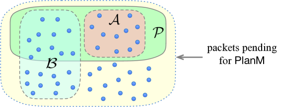
Figure 5.2: The sets of packets in the competitive analysis. The backup plan ${{\mathcal{B}}}$ is introduced in Section 5.2. It has the property that ${{\mathcal{P}}}\cap{{\mathcal{B}}}={{\mathcal{P}}}\setminus{{\mathcal{A}}}$.

Modifications of the adversary stash. We now overview the principles guiding the maintenance of the adversary stash ${{\mathcal{A}}}$. These principles are important in understanding the details of the analysis given in Sections 5.3-5.5. Let us fix some slot $\tau$ of ${{\mathcal{A}}}$. We describe all possible changes that the packet in slot $\tau$ of ${{\mathcal{A}}}$ can undergo in the course of the analysis and explain how we compensate the adversary for any such change, so that the total adversary credit from slot $\tau$ is at least $w^{0}({\textsf{OPT}}[\tau])$, as needed.

Adding packet ${\textsf{OPT}}[\tau]$ to ${{\mathcal{A}}}$. When packet $j={\textsf{OPT}}[\tau]$ arrives at a time $t$, if $j$ is added to the optimal plan ${{\mathcal{P}}}$ then we also add it to ${{\mathcal{A}}}$ in slot $\tau$. Otherwise, the slot $\tau$ remains empty in ${{\mathcal{A}}}$ all the time. In either case, the adversary does not get any credit for this packet at this time. (The credit of at least $w^{0}_{j}$ from slot $\tau$ will be awarded to the adversary later in the course of computation, possibly in smaller chunks. The strategy for amortizing this credit will be described shortly.)

Replacing packet ${{\mathcal{A}}}[\tau]$. Replacement of packets in ${{\mathcal{A}}}$ may occur in an iterated leap step when, under some circumstances, we replace a packet $h_{i}\in{{\mathcal{A}}}$ by $h_{i+1}$, which is always lighter than $h_{i}$ (see Lemma B.1(b)). To compensate her for this replacement, the adversary obtains credit equal to $w^{t}_{h_{i}}-w^{t+1}_{h_{i+1}}$, which is always non-negative.

To preserve invariant (InvA), when we make packet replacements, we need to make sure that no packet in ${{\mathcal{A}}}$ is scheduled after its current deadline, which requires some care for those packets whose deadlines were decreased. We also need to avoid adding into ${{\mathcal{A}}}$ a packet that is already in ${{\mathcal{A}}}$. Thus, before a packet $h_{i}\in{{\mathcal{A}}}$ gets replaced by $h_{i+1}$, we remove $h_{i+1}$ from its slot in ${{\mathcal{A}}}$ if it already belongs to this set.

Removing packet ${{\mathcal{A}}}[\tau]$ before step $\tau$. As mentioned above, in some cases we remove a packet $q={{\mathcal{A}}}[\tau]$ from ${{\mathcal{A}}}$ even though the current time has not reached $\tau$ yet. This is done in particular if $q$ is no longer in ${{\mathcal{P}}}$, due to being ousted or transmitted by the algorithm. However, in order to preserve certain invariants, we may also remove $q$ from ${{\mathcal{A}}}$ even if it remains in ${{\mathcal{P}}}$. If we remove packet $q={{\mathcal{A}}}[\tau]$ from ${{\mathcal{A}}}$ before step $\tau$, to compensate the adversary for this change, we give her the credit whose value is at least the difference (if positive) between the current weight of $q$ and the current value of ${\textsf{minwt}}({{\mathcal{P}}},\tau)$; the precise formula for this credit will be given below. Importantly, once we remove ${{\mathcal{A}}}[\tau]$ from ${{\mathcal{A}}}$, ${{\mathcal{A}}}[\tau]$ will remain empty forever.

Removing packet ${{\mathcal{A}}}[\tau]$ at time $\tau$. When processing the transmission event at time $\tau$, if there is a packet $j={A}^{\tau}[\tau]$ in slot $\tau$, we remove $j$ from ${{\mathcal{A}}}$ and the adversary gains its current weight, i.e., it obtains credit of $w^{\tau}_{j}$. It follows that ${{\mathcal{A}}}$ is empty after the last (transmission) event.

Weight and deadline changes. Increasing the weight of the substitute packet $\varrho$ in a leap step (line 4 of Algorithm PlanM) does not affect ${{\mathcal{A}}}$, as $\varrho$ is not in ${{\mathcal{P}}}$ and thus not in ${{\mathcal{A}}}$, by invariant (InvA). However, the algorithm also changes the weights and/or deadlines of some packets $h_{i}$ in an iterated leap step (line 11 of Algorithm PlanM), and these packets are in ${{\mathcal{P}}}$, so ${{\mathcal{A}}}$ might be affected too. To address this, in the analysis of an iterated leap step, we remove or replace all packets $h_{i}$ that are in ${{\mathcal{A}}}$ and the adversary gets credit based on their old weights. Some of the packets $h_{i}$ may be reinserted later in the analysis of the same step, but they are always reinserted with their new weights and deadlines. It follows that the weights of all packets in ${{\mathcal{A}}}$ are always current.

Amortization of the adversary profit. We now describe how the adversary profit of $w^{0}({\textsf{OPT}})$ is amortized. As already mentioned earlier, when a packet $j={\textsf{OPT}}[\tau]$ arrives at a time $t^{\prime}$, the adversary credit for $j$ may be awarded in smaller payments in steps $t^{\prime},t^{\prime}+1,...,\tau$. All the payments except the last one are called adjustment credits and the last one, in step $\tau$, is called the transmission credit. The formulas for these credits are given below.

We note that the adversary credit when processing the arrival of a packet $j$ is always $0$. This follows from two properties of the changes in ${{\mathcal{A}}}$: First, as explained above, the adversary does not receive credit for the arrival of $j$, whether it is added to ${{\mathcal{A}}}$ or not. Second, the only other change of ${{\mathcal{A}}}$ associated with the arrival of $j$ and the resulting modification of ${{\mathcal{P}}}$ may be a removal from ${{\mathcal{A}}}$ of some packet ${{\mathcal{A}}}[\tau]$ of weight at most ${\textsf{minwt}}({{\mathcal{P}}},\tau)$, for which the adversary does not get any credit (see below and Section 5.4).

In each step $t$, we define the adversary credit for step $t$, denoted $\textsf{advcredit}^{t}$, as the sum of the following two values:

• Transmission credit: This is the credit given to the adversary for her packet in slot $t$. More precisely, it is defined by

  $$\textsf{advcredit}^{t}_{t}\;=\;\left\{\begin{array}[]{lcl}w^{t}({{{A}}^{t}}[t])&&\text{if ${{{A}}^{t}}[t]$ is defined (not empty)}\\ {\textsf{minwt}}({{{P}}^{t}},t)&&\text{otherwise}\end{array}\right.$$

  Recall that $w^{t}({{{A}}^{t}}[t])$ represents the weight of ${{{A}}^{t}}[t]$ at time $t$, if ${{{A}}^{t}}[t]$ is defined.

• Adjustment credit: This is the credit that the adversary receives as compensation for modifications in ${{\mathcal{A}}}$. Namely, it is the sum of the following credits, one for each adjustment of ${{\mathcal{A}}}$ performed in the analysis of step $t$:

  • Adjustment credit for weight decreases: The difference between previous and new weight of ${{\mathcal{A}}}[\tau]$, for each slot $\tau\geq t$ where packet ${{\mathcal{A}}}[\tau]$ is replaced by a lighter packet.

  • Adjustment credit for packet removal: The value of $w^{t}_{q}-{\textsf{minwt}}({{{P}}^{t}},d^{t}_{q})$ for each packet $q={{\mathcal{A}}}[\tau]$ removed from ${{\mathcal{A}}}$.

  Before proceeding, we make two simple but important observations. First, all adjustment credits are non-negative. This is obvious for adjustment credits for weight decreases. As for the second type of adjustments, consider a packet $q={{\mathcal{A}}}[\tau]$ getting removed from ${{\mathcal{A}}}$ at time $t$. By invariant (InvA), we have that $q\in{{{P}}^{t}}$. Then the definition of function ${\textsf{minwt}}()$ implies that $w^{t}_{q}\geq{\textsf{minwt}}({{{P}}^{t}},d^{t}_{q})$; in other words the adjustment credits for packet removals are also non-negative.

  Second, observe that the formula above for the adjustment credit for packet removals is an upper bound on the actual loss of adversary’s future profit due to the removal of $q={{\mathcal{A}}}[\tau]$ from ${{\mathcal{A}}}$, which equals $\max{\{w^{t}_{q}-{\textsf{minwt}}({P}^{\tau},\tau),0\}}$ (as the transmission credit in step $\tau$ is ${\textsf{minwt}}({P}^{\tau},\tau)$). Indeed, we have ${\textsf{minwt}}({{{P}}^{t}},d^{t}_{q})\leq w^{t}_{q}$ and, since $\tau\leq d^{t}_{q}$, also ${\textsf{minwt}}({{{P}}^{t}},d^{t}_{q})\leq{\textsf{minwt}}({{{P}}^{t}},\tau)\leq{\textsf{minwt}}({P}^{\tau},\tau)$ by the slot-monotonicity property (Lemma 4.1). Therefore $w^{t}_{q}-{\textsf{minwt}}({{{P}}^{t}},d^{t}_{q})\geq\max{\{w^{t}_{q}-{\textsf{minwt}}({P}^{\tau},\tau),0\}}$. We use the value of $w^{t}_{q}-{\textsf{minwt}}({{{P}}^{t}},d^{t}_{q})$ here because it is sufficient for the analysis and easier to work with.

  At each step $t$, these credit adjustments (if any) may be performed in multiple substeps, with each substep involving processing some time interval $(\zeta,\eta]$. We will use notation $\textsf{advcredit}^{t}_{(\zeta,\eta]}$ for the adjustment credit resulting from modifications in the substep corresponding to time interval $(\zeta,\eta]$.

Claim 5.1.

The total adversary credit for all steps covers $w^{0}({\textsf{OPT}})$, that is,

$$w^{0}({\textsf{OPT}})\;\leq\;\sum_{t}\textsf{advcredit}^{t}\,,$$ (5.1)

where the sum is over all steps $t$.

Proof.

To prove (5.1), consider again a packet $j={\textsf{OPT}}[\tau]$ that arrived at some step $t^{\prime}$. It is sufficient to show that the sum of all adversary credits associated with slot $\tau$ for steps $t=t^{\prime},t^{\prime}+1,...,\tau$ is at least $w^{0}_{j}=w_{j}$.

At time $t^{\prime}$, if $j$ is added to ${{\mathcal{P}}}$, then $j$ is also added to ${{\mathcal{A}}}$; otherwise ${{\mathcal{A}}}[\tau]$ remains undefined. To streamline the proof, we think of the second case as adding $j$ to ${{\mathcal{A}}}$ in slot $\tau$ and then removing it immediately in the same step.

At any step $t$ when ${{\mathcal{A}}}[\tau]$ is defined, if the weight of ${{\mathcal{A}}}[\tau]$ is decreased, then, according to the definitions above, this decrease of weight contributes to the adjustment credit at step $t$. Consider the last step $t^{\prime\prime}$ when ${{\mathcal{A}}}[\tau]$ is defined, and let $q={{\mathcal{A}}}[\tau]$ be the packet in slot $\tau$ of ${{\mathcal{A}}}$ at that time. (It could be that $q\neq j$, as the packet in ${{\mathcal{A}}}[\tau]$ may change over time.) Then the total adjustment credit in steps $t^{\prime},t^{\prime}+1,\dots,t^{\prime\prime}-1$ for changing ${{\mathcal{A}}}[\tau]$ equals $w^{0}_{j}-w^{t^{\prime\prime}}_{q}$.

There are two cases. If $t^{\prime\prime}=\tau$, then the adversary will receive transmission credit of $\textsf{advcredit}^{\tau}_{\tau}=w^{\tau}_{q}$ in step $\tau$, and the right-hand side of (5.1) associated with slot $\tau$ (the sum of adjustment credits and the transmission credit for slot $\tau$) is $w^{0}_{j}-w^{\tau}_{q}+w^{\tau}_{q}=w^{0}_{j}$. If $t^{\prime\prime}<\tau$, then $q$ is removed from ${{\mathcal{A}}}$ in the analysis of step $t^{\prime\prime}$. The adjustment credits for steps $t=t^{\prime},t^{\prime}+1,\dots,t^{\prime\prime}-1$ add up to $w^{0}_{j}-w^{t^{\prime\prime}}_{q}$, and the adjustment credit in step $t^{\prime\prime}$ for removing $q$ from ${{\mathcal{A}}}$ is $w^{t^{\prime\prime}}_{q}-{\textsf{minwt}}({P}^{\prime\prime},d^{t^{\prime\prime}}_{q})$, where ${P}^{\prime\prime}$ is the snapshot of ${{\mathcal{P}}}$ when this removal of $q$ is taking place. Then later at step $\tau$ the adversary will receive transmission credit ${\textsf{minwt}}({P}^{\tau},\tau)$, by the definition above. Thus the total of adjustment and transmission credits associated with slot $\tau$ is at least

$$(\,w^{0}_{j}-w^{t^{\prime\prime}}_{q}\,)+(\,w^{t^{\prime\prime}}_{q}- {\textsf{minwt}}({P}^{\prime\prime},d^{t^{\prime\prime}}_{q})\,)+{\textsf{minwt}}({P}^{\tau},\tau)$$

$$\geq\;w^{0}_{j}-w^{t^{\prime\prime}}_{q}+(\,w^{t^{\prime\prime}}_{q}-{\textsf{minwt}}({P}^{\prime\prime},\tau)\,)+{\textsf{minwt}}({P}^{\prime\prime},\tau)$$ (5.2)

$$=\;w^{0}_{j},$$

where inequality (5.2) holds because ${\textsf{minwt}}({P}^{\prime\prime},d^{t^{\prime\prime}}_{q})\leq{\textsf{minwt}}({P}^{\prime\prime},\tau)$, by the definition of function ${\textsf{minwt}}()$ (see also the comments on adjustments credits for packet removals before Claim 5.1) and because ${\textsf{minwt}}({P}^{\tau},\tau)\geq{\textsf{minwt}}({P}^{\prime\prime},\tau)$, which follows from the slot monotonicity property, as summarized in Lemma 4.1. This concludes the proof of (5.1). ∎

5.2 Backup Plan and the Potential Function

In our analysis, we will maintain a set ${{\mathcal{B}}}$ of pending packets called a backup plan. ${{\mathcal{B}}}$ contains two types of packets: all packets in ${{\mathcal{P}}}\setminus{{\mathcal{A}}}$, and some pending packets not in ${{\mathcal{P}}}$. (The relation between ${{\mathcal{P}}}$, ${{\mathcal{B}}}$ and ${{\mathcal{A}}}$ is illustrated in Figure 5.2.) The packets in ${{\mathcal{B}}}\setminus{{\mathcal{P}}}$ will typically be packets that were earlier ousted from ${{\mathcal{P}}}$, either as a result of arrivals of other packets or in a leap step. These packets can also be thought of as candidates for the substitute packet $\textsf{sub}^{t}(p)$ when the algorithm chooses a packet $p$ for transmission.

The following invariant summarizes the essential properties of ${{\mathcal{B}}}$, and it will be maintained throughout the analysis:

(InvB) For any snapshot ${B}$ of ${{\mathcal{B}}}$ at any time $t$, (i) ${B}$ is a plan, i.e., a feasible set of packets pending in step $t$, and (ii) ${B}\cap{P}={P}\setminus{A}$, where ${P}$ and ${A}$ are the current snapshots of ${{\mathcal{P}}}$ and ${{\mathcal{A}}}$, respectively.

By Observation 3.1, invariant (InvB)(i) is equivalent to the condition that for any slot $\tau\geq t$, we have ${\textsf{pslack}}({B},\tau)\geq 0$. Invariant (InvB)(ii) and invariant (InvA) together imply that ${B}\cap{A}=\emptyset$ and ${{\mathcal{P}}}=({{\mathcal{P}}}\cap{{\mathcal{B}}})\cup{{\mathcal{A}}}$, i.e., that any packet in ${P}$ is either in ${A}$ or in ${B}$, but not in both. Similarly as for invariant (InvA), preserving invariant (InvB) in the course of the analysis will require making suitable changes in the adversary stash ${{\mathcal{A}}}$ and the backup plan ${{\mathcal{B}}}$.

The following observation is quite straightforward, but we state it explicitly here, as it is useful later in some proofs.

Observation 5.2.

Consider the current optimal plan ${P}$, the backup plan ${B}$, and the adversary stash ${A}$ at time $t$. Assume that invariants (InvA) and (InvB) hold. Let $\eta$ be a tight slot of ${P}$. Then:

1. ${A}(\eta,{T}]\neq\emptyset$ implies that ${B}(\eta,{T}]\setminus{P}\neq\emptyset$, and

2. ${B}[t,\eta]\setminus{P}\neq\emptyset$ implies that ${A}[t,\eta]\neq\emptyset$.

Proof.

(a) From the property that all plans are full and that $\eta$ is a tight slot of ${P}$, we have $|{P}(\eta,{T}]|={T}-\eta\leq|{B}(\eta,{T}]|$, where ${T}$ is the time horizon (see Section 3). Then, using invariants (InvA) and (InvB), we obtain that $|{A}(\eta,{T}]|=|{P}(\eta,{T}]\setminus{B}|\leq|{B}(\eta,{T}]\setminus{P}|$.

(b) Since $\eta$ is a tight slot of ${P}$ and ${B}$ is feasible, we have $|{P}[t,\eta]|=\eta-t+1\geq|{B}[t,\eta]|$. Therefore, if ${B}[t,\eta]\setminus{P}\neq\emptyset$, then ${P}[t,\eta]\setminus{B}\neq\emptyset$, which implies that ${A}[t,\eta]\neq\emptyset$, by invariant (InvB). ∎

The definitions of tight slots and segments apply to ${{\mathcal{B}}}$ (as well as to any plan), and they will be helpful in our proofs. We remark that ${{\mathcal{B}}}$ may have a different segment structure than the current optimal plan ${{\mathcal{P}}}$.

Before defining our potential function, we introduce a few lemmas that will be useful in showing that invariant (InvB) is preserved after each step.

Lemma 5.3.

Consider the current optimal plan ${P}$, the backup plan ${B}$, and the adversary stash ${A}$ at time $t$. Assume that invariants (InvA) and (InvB) hold, and let $\eta,\eta^{\prime}$ be two time slots such that $t\leq\eta\leq\eta^{\prime}$. Then

$${\textsf{pslack}}({P},\eta^{\prime})-{\textsf{pslack}}({P},\eta)+|{A}(\eta,\eta^{\prime}]|\;=\;{\textsf{pslack}}({B},\eta^{\prime})-{\textsf{pslack}}({B},\eta)+|{B}(\eta,\eta^{\prime}]\setminus{P}|\,.$$ (5.3)

Equation (5.3) may appear complicated, but it’s actually quite straightforward. It compares the contributions of the interval $(\eta,\eta^{\prime}]$ to ${\textsf{pslack}}()$ values of ${P}$ and ${B}$. These contributions differ by $-|{P}(\eta,\eta^{\prime}]|+|{B}(\eta,\eta^{\prime}]|$, and canceling out the common contribution $|{P}(\eta,\eta^{\prime}]\cap{B}|$ yields (5.3). A formal proof follows.

Proof.

(InvB) implies that ${A}(\eta,\eta^{\prime}]={P}(\eta,\eta^{\prime}]\setminus{B}$. Using the definition of ${\textsf{pslack}}()$, and canceling out the contributions of packets with deadline at most $\eta$, we get

$${\textsf{pslack}}({P},\eta^{\prime})-{\textsf{pslack}}({P},\eta)+|{A}(\eta,\eta^{\prime}]| =\;\eta^{\prime}-\eta-|{P}(\eta,\eta^{\prime}]|+|{P}(\eta,\eta^{\prime}]\setminus{B}|$$

$$=\;\eta^{\prime}-\eta-|{P}(\eta,\eta^{\prime}]\cap{B}|$$

$$=\;\eta^{\prime}-\eta-|{B}(\eta,\eta^{\prime}]|+|{B}(\eta,\eta^{\prime}]\setminus{P}|$$

$$=\;{\textsf{pslack}}({B},\eta^{\prime})-{\textsf{pslack}}({B},\eta)+|{B}(\eta,\eta^{\prime}]\setminus{P}|,$$

completing the proof. ∎

Lemma 5.4.

Consider the current optimal plan ${P}$, the backup plan ${B}$, and the adversary stash ${A}$ at time $t$. Assume that invariants (InvA) and (InvB) hold, and let $\zeta$ be a tight slot of ${P}$ (possibly, $\zeta=t-1$). Let ${f^{\ast}}$ be the earliest-deadline packet in ${B}(\zeta,{T}]\setminus{P}$ and let ${g^{\ast}}$ be the latest-deadline packet in ${A}[t,\zeta]$. (We allow here the possibility that ${f^{\ast}}$ or ${g^{\ast}}$ is undefined). Then:

1. If ${f^{\ast}}$ is defined, then ${\textsf{pslack}}({B},\tau)\geq{\textsf{pslack}}(P,\tau)+|{A}(\zeta,\tau]|$ for any $\tau\in(\zeta,d_{f^{\ast}})$. Otherwise this inequality holds for any $\tau>\zeta$.

2. If ${g^{\ast}}$ is defined, then ${\textsf{pslack}}({B},\tau)\geq{\textsf{pslack}}(P,\tau)+|{B}(\tau,\zeta]\setminus{P}|$ for any $\tau\in[d_{g^{\ast}},\zeta]$. Otherwise this inequality holds for any $\tau\in[t,\zeta]$.

Proof.

We first observe that, since ${B}$ is feasible and $\zeta$ is a tight slot for ${P}$, we have ${\textsf{pslack}}({B},\zeta)\geq 0={\textsf{pslack}}({P},\zeta)$.

(a) If packet ${f^{\ast}}$ exists, let $\theta=d_{f^{\ast}}$, otherwise let $\theta={T}+1$, where ${T}$ is the time horizon, as defined in Section 2. Let $\tau\in(\zeta,\theta)$. By the definition of ${f^{\ast}}$, there is no packet in ${B}\setminus{P}$ with deadline in $(\zeta,\theta)$; in particular ${B}(\zeta,\tau]\setminus{P}=\emptyset$. Using this, equation ${\textsf{pslack}}({P},\zeta)=0$, and Lemma 5.3 (with $\eta=\zeta$ and $\eta^{\prime}=\tau$), we obtain

$${\textsf{pslack}}({P},\tau)+|{A}(\zeta,\tau]|\;=\;{\textsf{pslack}}({B},\tau)-{\textsf{pslack}}({B},\zeta)\;\leq\;{\textsf{pslack}}({B},\tau)\,,$$

which implies claim (a).

(b) If packet ${g^{\ast}}$ exists, let $\lambda=d_{g^{\ast}}$, otherwise let $\lambda=t$. Let $\tau\in[\lambda,\zeta]$. By the definition of $\lambda$, there is no packet in ${A}$ with deadline in $(\lambda,\zeta]$, which implies that ${A}(\tau,\zeta]=\emptyset$. Using this, equation ${\textsf{pslack}}({P},\zeta)=0$, and Lemma 5.3 (with $\eta=\tau$ and $\eta^{\prime}=\zeta$), we obtain

$$-{\textsf{pslack}}({P},\tau)\;=\;{\textsf{pslack}}({B},\zeta)-{\textsf{pslack}}({B},\tau)+|{B}(\tau,\zeta]\setminus{P}|\,.$$

Using ${\textsf{pslack}}({B},\zeta)\geq 0$, we get $-{\textsf{pslack}}({P},\tau)\geq-{\textsf{pslack}}({B},\tau)+|{B}(\tau,\zeta]\setminus{P}|$ and claim (b) follows. ∎

In some cases of the analysis, we will have situations when a packet $g\in{{\mathcal{A}}}$ needs to be removed from ${{\mathcal{A}}}$. By the definition of the backup plan, this causes $g$ to be added to ${{\mathcal{B}}}$, making ${{\mathcal{B}}}$ infeasible. The lemma below shows that we can restore the feasibility of ${{\mathcal{B}}}$ after such a change by removing from ${{\mathcal{B}}}$ a suitably chosen packet that is not in ${{\mathcal{P}}}$.

Lemma 5.5.

Consider the current optimal plan ${P}$, the backup plan ${B}$, and the adversary stash ${A}$ at time $t$. Assume that invariants (InvA) and (InvB) hold. Let $g\in{A}$, $\eta=\textsf{prevts}({P},d_{g})$, and $\eta^{\prime}=\textsf{nextts}({B},d_{g})$. Then

(a) ${B}(\eta,\eta^{\prime}]\setminus{P}\neq\emptyset$.

(b) For any $f\in{B}(\eta,\eta^{\prime}]\setminus{P}$, the set $C={B}\setminus{\left\{f\right\}}\cup{\left\{g\right\}}$ is feasible and $w_{f}\leq w_{g}$ (thus $w(C)\geq w({B})$).

Proof.

Note that the choice of $g\in{A}$ implies that $g\notin{B}$. We use Lemma 5.3 with $\eta$ and $\eta^{\prime}$ as defined here. We can apply this lemma because ${B}$ satisfies invariant (InvB). From that lemma, substituting ${\textsf{pslack}}({P},\eta)={\textsf{pslack}}({B},\eta^{\prime})=0$, we get

$${\textsf{pslack}}({P},\eta^{\prime})+|{A}(\eta,\eta^{\prime}]|\;=\;-{\textsf{pslack}}({B},\eta)+|{B}(\eta,\eta^{\prime}]\setminus{P}|\;\leq\;|{B}(\eta,\eta^{\prime}]\setminus{P}|\,,$$

where the last inequality follows from ${\textsf{pslack}}({B},\eta)\geq 0$, which is a consequence of the feasibility of ${B}$. The existence of $g$ implies ${A}(\eta,\eta^{\prime}]\neq\emptyset$, and hence, using the feasibility of ${P}$, we obtain that ${B}(\eta,\eta^{\prime}]\setminus{P}\neq\emptyset$ holds as well, proving claim (a).

Pick any $f\in{B}(\eta,\eta^{\prime}]\setminus{P}$. From $d_{f}\leq\eta^{\prime}=\textsf{nextts}({B},d_{g})$ we obtain that $C$ is feasible. Inequality $d_{f}>\eta=\textsf{prevts}({P},d_{g})$ and $f\not\in{P}$ imply that $w_{f}\leq{\textsf{minwt}}({P},d_{g})\leq w_{g}$, and therefore $w(C)\geq w({B})$, completing the proof of claim (b). ∎

As a corollary, we obtain that Lemma 5.5(b) holds for $f$ equal to the earliest-deadline packet ${f^{\ast}}$ in ${B}\setminus{P}$ with $d_{f^{\ast}}>\textsf{prevts}({P},d_{g})$.

Corollary 5.6.

Consider the current optimal plan ${P}$, the backup plan ${B}$, and the adversary stash ${A}$ at time $t$. Assume that invariants (InvA) and (InvB) hold. Let $g\in{A}$, $\eta=\textsf{prevts}({P},d_{g})$, and let ${f^{\ast}}$ be the earliest-deadline packet in ${B}(\eta,{T}]\setminus{P}$. Then packet ${f^{\ast}}$ exists, the set $C={B}\setminus{\left\{{f^{\ast}}\right\}}\cup{\left\{g\right\}}$ is feasible, and $w_{f^{\ast}}\leq w_{g}$ (thus $w(C)\geq w({B})$).

Proof.

Applying Lemma 5.5(a) to packet $g$ and $\eta^{\prime}=\textsf{nextts}({B},d_{g})$ gives us that ${B}(\eta,\eta^{\prime}]\setminus{P}\neq\emptyset$, which in turn implies that $d_{f^{\ast}}\in(\eta,\eta^{\prime}]$. Then, using Lemma 5.5(b) for $f={f^{\ast}}$ implies the corollary. ∎

Potential function. We use the backup plan ${{\mathcal{B}}}$ to define a potential function needed for the amortized analysis of Algorithm PlanM. If ${B}$ is the current snapshot of ${{\mathcal{B}}}$ then the potential value at time $t$ is

$$\textstyle\Psi({B})\;=\;\frac{1}{\phi}{\,}w^{t}({B})\,.$$ (5.4)

For brevity, we will use notation ${\widetilde{\Psi}^{t}}=\Psi({\widetilde{{B}}^{t}})$ for the potential at the beginning of step $t$, before any packet arrives, and ${\Psi^{t}}=\Psi({{{B}}^{t}})$ for the potential just before a packet is transmitted in step $t$.

The intuition behind this definition is as follows. In order to be $\phi$-competitive, the average (per step) profit of Algorithm PlanM should be at least $1/\phi$ times the adversary’s average profit. However, due to the choice of coefficients in line 1 of the algorithm, Algorithm PlanM tends to postpone transmitting heavy packets with large deadlines. (For example, given just two packets, a tight packet with weight $1$ and a non-tight packet with weight $2.6<\phi^{2}$, the algorithm will transmit the tight packet in the current step.) As a result, in tight instances, PlanM’s actual profit per step, throughout most of the game, is often smaller than $1/\phi$ times the adversary’s, and only near the end of the instance, when delayed heavy packets are transmitted, the algorithm can make up for this deficit.

In our amortized analysis, if there is a deficit in a given step, we pay for it with a “loan” that is represented by an appropriate increase of the potential function. Eventually, of course, these loans need to be repaid – the potential eventually decreases to $0$ and this decrease must be covered by excess profit. The formula for the potential $\Psi$ is designed to guarantee such future excess profits. To see this, imagine that no more packets arrive. Since ${{\mathcal{B}}}\cap{{\mathcal{A}}}=\emptyset$, the packets in ${{\mathcal{B}}}$ will not be transmitted in the future by the adversary. If the algorithm does not execute any more leap steps then it will collect all the packets in ${{\mathcal{P}}}$, which are in total heavier than the packets in ${{\mathcal{B}}}$ (as ${{\mathcal{B}}}$ is feasible by invariant (InvB)(i) and each packet $f\in{{\mathcal{B}}}\setminus{{\mathcal{P}}}$ satisfies $w^{t}_{f}\leq{\textsf{minwt}}({{\mathcal{P}}},d^{t}_{f})$ at each time step $t$). On the other hand, if the algorithm executes a leap step, instead of a packet ousted from ${{\mathcal{P}}}$ in this step, the algorithm will collect a packet from ${{\mathcal{B}}}\setminus{{\mathcal{P}}}$ (or a better packet) after it is added to the optimal plan as a substitute packet.

5.3 Overview of the Analysis

This section gives an overview of the analysis, states the main theorem, and shows how it follows from results that will be established in the sections that follow.

Initial and final state. At the beginning, per assumption (A1), we assume that the optimal plan is pre-filled with virtual $0$-weight packets, each in a slot equal to its deadline, and none of them scheduled by the adversary for transmission. The adversary stash ${{\mathcal{A}}}$ is empty, i.e., before the first step (at time $0$) we have $\widetilde{{A}}^{0}=\emptyset$, and the backup plan is the same as the optimal plan, i.e., $\widetilde{{B}}^{0}=\widetilde{{P}}^{0}$. Thus invariants (InvA) and (InvB) clearly hold, and $\widetilde{\Psi}^{0}=0$. At the end, after all (non-virtual) packets expire, the potential equals $0$ as well, i.e., $\widetilde{\Psi}^{{T}+1}=0$, where ${T}$ is the time horizon (the last step).

Amortized analysis. At the core of our analysis are bounds relating amortized profits of the algorithm and the adversary in each step $t$. For packet arrivals in step $t$, we will show the following packet-arrivals inequality:

$${\Psi^{t}}-{\widetilde{\Psi}^{t}}\geq 0\,.$$ (5.5)

For the transmission event in a step $t$, we will show that the following packet-transmission inequality holds:

$$\phi{\,}w^{t}({\textsf{ALG}}[t])-\phi{\,}(\Delta^{t}{w})+({\widetilde{\Psi}^{t+1}}-{\Psi^{t}})\;\geq\;\textsf{advcredit}^{t},$$ (5.6)

where ${\textsf{ALG}}[t]$ is the packet in slot $t$ in the algorithm’s schedule ALG (thus $w^{t}({\textsf{ALG}}[t])$ is the algorithm’s profit), and $\Delta^{t}{w}$ is the total amount by which the algorithm increases the weights of its pending packets in step $t$.

We prove the packet-arrivals inequality (5.5) in Section 5.4 and the packet-transmission inequality (5.6) in Section 5.5. Assuming that these two inequalities hold, we now show our main result.

Theorem 5.7.

Algorithm PlanM is $\phi$-competitive.

Proof.

We show that $\phi{\,}w^{0}({\textsf{ALG}})\geq w^{0}({\textsf{OPT}})$, which implies the theorem. First, by Claim 5.1, we have $w^{0}({\textsf{OPT}})\leq\sum_{t}\textsf{advcredit}^{t}$. Second, note that

$$\sum_{t}\,(\,{\widetilde{\Psi}^{t+1}}-{\widetilde{\Psi}^{t}}\,)\;=\;\widetilde{\Psi}^{T+1}-\widetilde{\Psi}^{0}\;=\;0\,,$$ (5.7)

where $\widetilde{\Psi}^{0}=0$ is the initial potential and $\widetilde{\Psi}^{{T}+1}=0$ is the final potential after the last step ${T}$. Observe also that

$$\sum_{t}[\,w^{t}(\textsf{ALG}[t])-\Delta^{t}{w}\,]\;\leq\;w^{0}(\textsf{ALG})\,.$$ (5.8)

This follows from the observation that if the weight of $\textsf{ALG}[\tau]$ was increased by some value $\delta>0$ at some step $t^{\prime}<\tau$, then $\delta$ also contributes to $\Delta^{t^{\prime}}{w}$, so such contributions cancel out in (5.8). (There may be several such $\delta$’s, as the weight of a packet may have been increased multiple times. Note that the bound (5.8) may not be tight if some packets with increased weights are later dropped.)

Summarizing, using the above bounds yields

$$w^{0}({\textsf{OPT}})\; \leq\;\sum_{t}\textsf{advcredit}^{t}$$ (5.9)

$$\leq\;\sum_{t}\Big{[}\phi{\,}w^{t}(\textsf{ALG}[t])-\phi{\,}(\Delta^{t}{w})+({\widetilde{\Psi}^{t+1}}-{\Psi^{t}})\Big{]}+\sum_{t}({\Psi^{t}}-{\widetilde{\Psi}^{t}})$$ (5.10)

$$=\;\sum_{t}\Big{[}\phi{\,}w^{t}(\textsf{ALG}[t])-\phi{\,}(\Delta^{t}{w})\Big{]}+\sum_{t}({\widetilde{\Psi}^{t+1}}-{\widetilde{\Psi}^{t}})$$

$$\leq\;\phi{\,}w^{0}(\textsf{ALG})\,,$$ (5.11)

where inequality (5.9) is (5.1), inequality (5.10) follows by applying (5.5) and (5.6) for each step $t$, and inequality (5.11) holds by (5.7) and (5.8). ∎

5.4 Packet Arrivals

Let $t$ be the current time step. Our aim in this section is to prove that invariants (InvA) and (InvB) can be preserved as packets arrive in step $t$, using appropriate modifications of sets ${{\mathcal{A}}}$ and ${{\mathcal{B}}}$. We also prove that the packet-arrivals inequality (5.5) holds for step $t$. To this end, it is sufficient to show how to preserve both invariants, without decreasing the value of $w({{\mathcal{B}}})$ (and thus $\Psi$ as well), in response to an arrival of each individual packet.

Thus, consider the arrival event of a packet $s$ at time $t$. Let ${P}$ be the optimal plan just before $s$ arrives and let ${Q}$ be the optimal plan just after $s$ arrives. Furthermore, let ${A}$ and ${B}$ be the snapshots of ${{\mathcal{A}}}$ and ${{\mathcal{B}}}$ just before $s$ arrives, and let ${A}_{+s}$ and ${B}_{+s}$ denote, respectively, the snapshots of ${{\mathcal{A}}}$ and ${{\mathcal{B}}}$ just after $s$ arrives and the changes described below are applied. The algorithm does not change the weights and deadlines after packet arrivals, so we will omit the superscript $t$ in the notation for weights and deadlines, that is $w_{q}=w^{t}_{q}$ and $d_{q}=d^{t}_{q}$, for each packet $q$. There are two cases, depending on whether or not $s\in{Q}$.

Case A.1: $s$ is not added to the optimal plan ${{\mathcal{P}}}$, i.e., ${Q}={P}$. Lemma A.2 implies that $w_{s}<{\textsf{minwt}}({P},d_{s})={\textsf{minwt}}({Q},d_{s})$. In this case, we do not change ${{\mathcal{A}}}$, i.e., ${A}_{+s}={A}$, so invariant (InvA) is preserved. The backup plan ${{\mathcal{B}}}$ remains the same as well, so $w({{\mathcal{B}}})$ does not change and invariant (InvB) is preserved.

Case A.2: $s$ is added to the optimal plan ${{\mathcal{P}}}$. Let $u$ be the lightest packet in ${P}$ with $d_{u}\leq\textsf{nextts}({P},d_{s})$; by assumption (A1) such $u$ exists. By the choice of $u$ and Lemma A.2, we have ${Q}={P}\cup{\left\{s\right\}}\setminus{\left\{u\right\}}$, $\textsf{nextts}({P},d_{u})\leq\textsf{nextts}({P},d_{s})$, and $w_{s}>w_{u}={\textsf{minwt}}({P},d_{s})={\textsf{minwt}}({P},d_{u})$.

Replacing $u$ by $s$ in ${{\mathcal{P}}}$ can also trigger changes in ${{\mathcal{A}}}$ and ${{\mathcal{B}}}$. We describe these changes in two parts:

(i) First, we show that if $u\in{A}$, then we can remove $u$ from ${{\mathcal{A}}}$, preserving the invariants and not decreasing the potential.

(ii) Then, assuming that $u\notin{{\mathcal{A}}}$, we describe and analyze the remaining changes.

Let ${A}_{\mathrm{(i)}}$ denote the intermediate adversary stash, after the change in (i) and before the change in (ii), where we let ${A}_{\mathrm{(i)}}={A}$ if $u\notin{A}$, that is when change (i) does not apply. We adopt the same notation for snapshots of set ${{\mathcal{B}}}$.

(i) Dealing with $u\in{A}$. In this case we need to remove $u$ from ${{\mathcal{A}}}$, to preserve invariant (InvA). But this also forces us to add $u$ to ${{\mathcal{B}}}$, in order to preserve (InvB)(ii), which in turn requires removing some packet from ${{\mathcal{B}}}$ to preserve its feasibility.

To implement these changes, we use Lemma 5.5 with $g=u$, which gives us that there is a packet $f_{u}\in{B}\setminus{P}$ such that the set ${B}\setminus{\left\{f_{u}\right\}}\cup{\left\{u\right\}}$ is feasible and $w({B}\setminus{\left\{f_{u}\right\}}\cup{\left\{u\right\}})\geq w({B})$. We then let

$${A}_{\mathrm{(i)}}\;=\;{A}\setminus{\left\{u\right\}}\quad\textrm{and}\quad{B}_{\mathrm{(i)}}\;=\;{B}\setminus{\left\{f_{u}\right\}}\cup{\left\{u\right\}}.$$

Since $u$ is scheduled in $A$ in interval $[t,d_{u}]$ and $w_{u}={\textsf{minwt}}({P},d_{u})$, the adversary adjustment credit associated with removing $u$ from ${{\mathcal{A}}}$ is $w_{u}-{\textsf{minwt}}({P},d_{u})=0$ (see Section 5.1). As explained above, we also have that ${B}_{\mathrm{(i)}}$ is feasible and $w({B}_{\mathrm{(i)}})\geq w({B})$; thus invariant (InvB) is preserved and the change of $w({{\mathcal{B}}})$ is non-negative.

(ii) Analysis of other changes. By (i) we can now assume that $u\notin{A}_{\mathrm{(i)}}$, and invariant (InvB)(ii) together with $u\in{P}$ imply that $u\in{B}_{\mathrm{(i)}}$. We now consider the changes of ${{\mathcal{B}}}$ resulting from including $s$ in ${{\mathcal{P}}}$. We analyze two subcases, depending on whether or not $s\in{\textsf{OPT}}$.

Case A.2.a: $s\in{\textsf{OPT}}$. We add $s$ to ${{\mathcal{A}}}$ in the same slot as in OPT. Specifically, we take ${A}_{+s}={A}_{\mathrm{(i)}}\cup{\left\{s\right\}}$ and ${B}_{+s}={B}_{\mathrm{(i)}}$. Invariant (InvA) is preserved as $s\in{A}_{+s}$, invariant (InvB) holds as ${{\mathcal{B}}}$ remains unaffected in (ii), and the value of $w({{\mathcal{B}}})$ does not change.

Case A.2.b: $s\notin{\textsf{OPT}}$. In this case, we simply let ${A}_{+s}={A}_{\mathrm{(i)}}$, so invariant (InvA) continues to hold. However, $s$ needs to get added to ${{\mathcal{B}}}$ to preserve invariant (InvB)(ii), so we need to remove some packet from ${{\mathcal{B}}}$ to maintain its feasibility, and this packet must be lighter than $s$ to assure that the potential does not decrease. Define $\xi=\textsf{nextts}({P},d_{s})$ and $\xi_{{B}}=\textsf{nextts}({B}_{\mathrm{(i)}},d_{s})$. We have two cases.

If $d_{u}\leq\xi_{{B}}$, we replace $u$ by $s$ in ${{\mathcal{B}}}$. That is, we let ${B}_{+s}={B}_{\mathrm{(i)}}\cup{\left\{s\right\}}\setminus{\left\{u\right\}}$, and this satisfies invariant (InvB)(ii). The case condition implies that invariant (InvB)(i) continues to hold, and, as $w_{u}<w_{s}$ in Case A.2, the value of $w({{\mathcal{B}}})$ does not decrease.

Next, assume that $d_{u}>\xi_{{B}}$. Note that $d_{u}\leq\xi$, by the definition of $u$. Let $\lambda=\textsf{prevts}({P},d_{s})$. In this case we have that $\lambda<d_{s}\leq\xi_{{B}}<d_{u}\leq\xi$, so $d_{u}$ and $d_{s}$ are in the same segment $(\lambda,\xi]$ of ${P}$. Since $\lambda$ is a tight slot for ${P}$, $\xi_{{B}}$ is a tight slot for ${B}_{\mathrm{(i)}}$, and ${\textsf{pslack}}({P},\xi_{{B}})>0$, from Lemma 5.3 with $\eta=\lambda$ and $\eta^{\prime}=\xi_{{B}}$ we get that

$$|{B}_{\mathrm{(i)}}(\lambda,\xi_{{B}}]\setminus{P}|\;=\;{\textsf{pslack}}({B}_{\mathrm{(i)}},\lambda)+{\textsf{pslack}}({P},\xi_{{B}})+|{A}_{\mathrm{(i)}}(\lambda,\xi_{{B}}]|\;>\;0\,,$$

implying ${B}_{\mathrm{(i)}}(\lambda,\xi_{{B}}]\setminus{P}\neq\emptyset$. Choose any $f\in{B}_{\mathrm{(i)}}(\lambda,\xi_{{B}}]\setminus{P}$ and let ${B}_{+s}={B}_{\mathrm{(i)}}\cup{\left\{s\right\}}\setminus{\left\{f\right\}}$, preserving invariant (InvB)(ii). Invariant (InvB)(i) holds for ${B}_{+s}$ because $d_{f}\leq\xi_{{B}}=\textsf{nextts}({B}_{\mathrm{(i)}},d_{s})$. The optimality of ${P}$ and the choice of $u$ and $f$ imply that $w_{f}\leq{\textsf{minwt}}({P},d_{s})=w_{u}<w_{s}$, thus $w({{\mathcal{B}}})$ cannot decrease.

Summarizing, we showed that in response to the arrival of any packet $s$ in step $t$ we can modify ${{\mathcal{A}}}$ and ${{\mathcal{B}}}$ in such a way that the invariants (InvA) and (InvB) will be preserved and the value of $\Psi$ will not decrease. This gives us that the packet-arrivals inequality (5.5) holds for step $t$ and that after packet arrivals both invariants (InvA) and (InvB) will hold, concluding the analysis of packet arrivals in step $t$.

5.5 Transmitting a Packet

Let $t$ be the current step of the computation. After all packets with release time equal to $t$ arrive, the algorithm transmits its packet $p={\textsf{ALG}}[t]$. Recall that ${{{P}}^{t}}$ is the optimal plan just before transmitting $p$ and ${\widetilde{{P}}^{t+1}}$ is the optimal plan after the algorithm transmits $p$, possibly adjusts weights and deadlines, and after the time is incremented to $t+1$.

We split the analysis of the transmission step into two parts, called the adversary step and the algorithm’s step, defined as follows:

Adversary step: If packet ${{{A}}^{t}}[t]$ is defined, say ${{{A}}^{t}}[t]=j$, then we need to remove it from ${{\mathcal{A}}}$. (Recall that packets in ${{\mathcal{A}}}$ may have been removed or replaced during the analysis, so $j$ may not be equal to ${\textsf{OPT}}[t]$, the packet scheduled in OPT at time $t$.) Removing $j$ from ${{\mathcal{A}}}$ could trigger a change in ${{\mathcal{B}}}$, but the optimal plan ${{\mathcal{P}}}$ remains unchanged. We show that these changes preserve both invariants (InvA) and (InvB). We should stress that these changes are made without advancing the current time, which will be done in algorithm’s step.

In the analysis of the adversary step, given in Section 5.5.1, we establish a relation (inequality (5.12)) between the adversary transmission credit and the change of the potential. By ${{{A}}^{t}_{{\mathrm{adv}}}}$ and ${{{B}}^{t}_{{\mathrm{adv}}}}$ we will denote the snapshots of sets ${{\mathcal{A}}}$ and ${{\mathcal{B}}}$, respectively, right after the adversary step.

Algorithm’s step: In the algorithm’s step, the algorithm transmits $p$, the time is incremented to $t+1$, and the optimal plan changes from ${{{P}}^{t}}$ to ${\widetilde{{P}}^{t+1}}$.

The analysis of this step assumes that the changes described in the adversary step have already been implemented. Using the bound (5.12), invariants (InvA) and (InvB), and other properties, we then show that the packet-transmission inequality (5.6) holds after the sets ${{\mathcal{P}}}$, ${{\mathcal{A}}}$, and ${{\mathcal{B}}}$ are updated to reflect the changes triggered by the packet’s transmission. We also ensure that invariants (InvA) and (InvB) are preserved.

The analysis of the algorithm’s step is given in Sections 5.5.2-5.5.6. We first analyze the ordinary step in Section 5.5.2. We then give a roadmap for the analysis of a leap step in Section 5.5.3, as it will be divided into substeps. We analyze the particular substeps in Section 5.5.4, which describes the changes in the initial segment $[t,\alpha]$ of ${{{P}}^{t}}$, and in Sections 5.5.5-5.5.6, which contain the analysis of other changes resulting from a leap step.

In Table 1, we summarize the notation of snapshots that we use in this section.

Set description				Optimal plan	Backup plan	Adversary stash
Dynamic set				${{\mathcal{P}}}$	${{\mathcal{B}}}$	${{\mathcal{A}}}$
Beginning of step $t$ (before packet arrivals)				${\widetilde{{P}}^{t}}$	${\widetilde{{B}}^{t}}$	${\widetilde{{A}}^{t}}$
Before transmission in step $t$ (after packet arrivals)				${{{P}}^{t}}$	${{{B}}^{t}}$	${{{A}}^{t}}$
Transmission event in step $t$	After the adversary step (Sec. 5.5.1)			${{{P}}^{t}}$	${{{B}}^{t}_{{\mathrm{adv}}}}$	${{{A}}^{t}_{{\mathrm{adv}}}}$
	Leap step (Sec. 5.5.3)	After processing $[t,\alpha]$ and incrementing time (Sec. 5.5.4)		${{{P}}^{t+1}_{{\mathrm{ins}}}}$	${{{B}}^{t+1}_{{\mathrm{ins}}}}$	${{{A}}^{t+1}_{{\mathrm{ins}}}}$
		Iterated leap step (Sec. 5.5.6)	Before stage for group ${\langle a,b\rangle}$	${\dot{{P}}^{t+1}_{{\langle a,b\rangle}}}$	${\dot{{B}}^{t+1}_{{\langle a,b\rangle}}}$	${\dot{{A}}^{t+1}_{{\langle a,b\rangle}}}$
			After stage for group ${\langle a,b\rangle}$	${\ddot{{P}}^{t+1}_{{\langle a,b\rangle}}}$	${\ddot{{B}}^{t+1}_{{\langle a,b\rangle}}}$	${\ddot{{A}}^{t+1}_{{\langle a,b\rangle}}}$
Local notation (after part (i) of changes)				${{{P}}^{t}_{(i)}}$	${{{B}}^{t}_{(i)}}$	${{{A}}^{t}_{(i)}}$

Table 1: Notation of snapshots of sets ${{\mathcal{P}}},{{\mathcal{B}}}$, and ${{\mathcal{A}}}$ used in the analysis. The particular snapshots for each substep of the analysis of a leap step will be defined later, in the respective sections.

5.5.1 Adversary Step

As defined in Section 5.1, if ${{{A}}^{t}}$ contains a packet in slot $t$, then the adversary gains the transmission credit of $\textsf{advcredit}^{t}_{t}=w^{t}({{{A}}^{t}}[t])$. Otherwise, the adversary’s transmission credit equals $\textsf{advcredit}^{t}_{t}={\textsf{minwt}}({{{P}}^{t}},t)$. (The overall adversary credit for this step also includes the adjustment credit, but in this section we focus only on the relation between the transmission credit and the potential change in the adversary step.)

Except for possibly removing packet ${{{A}}^{t}}[t]$ from ${{\mathcal{A}}}$, if it is defined, we will not make other changes to ${{\mathcal{A}}}$, so invariant (InvA) will be preserved. Below we show that with appropriate changes invariant (InvB) will also be preserved after the adversary step. Further, denoting by $\Delta_{{\mathrm{adv}}}\Psi$ the change of the potential in the adversary step, we prove the following auxiliary inequality:

$$\Delta_{{\mathrm{adv}}}\Psi-\textsf{advcredit}^{t}_{t}\;\geq\;-{\textstyle{\frac{1}{\phi^{2}}}}{\,}{w^{t}_{p}}-{\textstyle{\frac{1}{\phi}}}{\,}{w^{t}(\textsf{sub}^{t}(p))}\,.$$ (5.12)

Recall that throughout Section 5.5 we denote the packet scheduled by the algorithm in step $t$ by $p$.

The proof of inequality (5.12) is divided into two cases, depending on whether or not ${{{A}}^{t}}[t]$ is defined. As packet weights are not changed in the adversary step, below we omit the superscript $t$ in the notation for weights.

Case ADV.1: ${{{A}}^{t}}$ contains a packet in slot $t$. Let $j={{{A}}^{t}}[t]$. We will now remove $j$ from the adversary stash ${{\mathcal{A}}}$ and, since by invariant (InvA) we have $j\in{{{P}}^{t}}$, we need to add packet $j$ to the backup plan ${{\mathcal{B}}}$ to maintain invariant (InvB)(ii), which in turn requires removing a packet from ${{\mathcal{B}}}$ to preserve its feasibility. To this end, we apply Lemma 5.5 (with $g=j$), which implies that there is a packet $f_{j}\in{{{B}}^{t}}\setminus{{{P}}^{t}}$ such that $d_{f_{j}}>\textsf{prevts}({{{P}}^{t}},d_{j})$, $w_{f_{j}}\leq w_{j}$, and for which set ${{{B}}^{t}}\setminus{\left\{f_{j}\right\}}\cup{\left\{j\right\}}$ is feasible.

We thus set ${{{A}}^{t}_{{\mathrm{adv}}}}={{{A}}^{t}}\setminus{\left\{j\right\}}$ and ${{{B}}^{t}_{{\mathrm{adv}}}}={{{B}}^{t}}\setminus{\left\{f_{j}\right\}}\cup{\left\{j\right\}}$. Invariant (InvA) is clearly preserved, and by Lemma 5.5, invariant (InvB) continues to hold as well. The potential change is

$$\Delta_{{\mathrm{adv}}}\Psi\;=\;{\textstyle{\frac{1}{\phi}}}{\,}\left(w({{{B}}^{t}_{{\mathrm{adv}}}})-w({{{B}}^{t}})\right)\;=\;{\textstyle{\frac{1}{\phi}}}{\,}(-w_{f_{j}}+w_{j}).$$ (5.13)

From the definition of $\textsf{sub}^{t}(j)$, $d_{f_{j}}>\textsf{prevts}({{{P}}^{t}},d_{j})$, and $f_{j}\notin{{{P}}^{t}}$, we have that $f_{j}$ is a candidate for $\textsf{sub}^{t}(j)$, and thus $w(\textsf{sub}^{t}(j))\geq w_{f_{j}}$. Using (5.13) and $\textsf{advcredit}^{t}_{t}=w_{j}$, it follows that

$$\phi{\,}(\,\Delta_{{\mathrm{adv}}}\Psi-\textsf{advcredit}^{t}_{t}\,)\; =\;-w_{f_{j}}+w_{j}-\phi{\,}w_{j}$$

$$=\;-{\textstyle{\frac{1}{\phi}}}{\,}{w_{j}}-w_{f_{j}}$$

$$\geq\;-{\textstyle{\frac{1}{\phi}}}{\,}{w_{j}}-{w(\textsf{sub}^{t}(j))}$$

$$\geq\;-{\textstyle{\frac{1}{\phi}}}{\,}{w_{p}}-{w(\textsf{sub}^{t}(p))}\,,$$ (5.14)

where inequality (5.14) follows from the choice of $p$ in line 1 of the algorithm’s description, using also that $j\in{{{P}}^{t}}$. This implies (5.12).

Case ADV.2: Slot $t$ is empty in ${{{A}}^{t}}$. In this case, we do not change ${{\mathcal{A}}}$ and ${{\mathcal{B}}}$, so ${{{A}}^{t}_{{\mathrm{adv}}}}={{{A}}^{t}}$ and ${{{B}}^{t}_{{\mathrm{adv}}}}={{{B}}^{t}}$. Invariants (InvA) and (InvB) are trivially preserved. Recall that $\textsf{advcredit}^{t}_{t}={\textsf{minwt}}({{{P}}^{t}},t)=w_{\ell}$, where ${\ell}$ denotes the lightest packet in the initial segment of ${{{P}}^{t}}$. Note that $\textsf{sub}^{t}({\ell})={\ell}$ and that $\Delta_{{\mathrm{adv}}}\Psi=0$. Then

$$\phi{\,}(\,\Delta_{{\mathrm{adv}}}\Psi-\textsf{advcredit}^{t}_{t}\,)\; =\;-\phi{\,}w_{\ell}$$

$$=\;-{\textstyle{\frac{1}{\phi}}}{\,}{w_{\ell}}-w(\textsf{sub}^{t}({\ell}))$$

$$\geq\;-{\textstyle{\frac{1}{\phi}}}{\,}{w_{p}}-w(\textsf{sub}^{t}(p))\,,$$ (5.15)

where inequality (5.15) follows from the choice of $p$ again. Thus (5.12) holds.

This concludes the analysis of the adversary step. In particular, we have determined the snapshots ${{{A}}^{t}_{{\mathrm{adv}}}}$ and ${{{B}}^{t}_{{\mathrm{adv}}}}$, of the adversary stash ${{\mathcal{A}}}$ and the backup plan ${{\mathcal{B}}}$, respectively, resulting from the adversary step. Next, in the following sections, we analyze the algorithm’s step.

5.5.2 Ordinary Step

We now assume that the adversary step, as described in the previous section, has already been implemented. The current optimal plan ${{{P}}^{t}}$ remains unchanged in the adversary step, and the current snapshots of ${{\mathcal{A}}}$ and ${{\mathcal{B}}}$ are ${{{A}}^{t}_{{\mathrm{adv}}}}$ and ${{{B}}^{t}_{{\mathrm{adv}}}}$. In this section we analyze the algorithm’s move at step $t$, assuming this is an ordinary step, as defined in Section 4.

In an ordinary step a packet $p\in{{{P}}^{t}}[t,\alpha]$ is transmitted, where $\alpha=\textsf{nextts}^{t}(t)$ is the first tight slot in ${{{P}}^{t}}$. The algorithm makes no changes in packet weights and deadlines, so $\Delta^{t}{w}=0$. Thus, to simplify notation, for any packet $q$ we can write $w_{q}=w^{t}_{q}$ and $d_{q}=d^{t}_{q}$, omitting the superscript $t$. As usual, ${\ell}$ denotes the lightest packet in the initial segment ${{{P}}^{t}}[t,\alpha]$.

By the algorithm, $p$ is the heaviest packet in ${{{P}}^{t}}[t,\alpha]$. Since $\textsf{sub}^{t}(p)={\ell}$, inequality (5.12) gives us that

$$\Delta_{{\mathrm{adv}}}\Psi-\textsf{advcredit}^{t}_{t}\;\geq\;-{\textstyle{\frac{1}{\phi^{2}}}}{\,}{w_{p}}-{\textstyle{\frac{1}{\phi}}}{\,}w_{\ell}\,.$$ (5.16)

According to Lemma A.4, the new optimal plan (starting at time slot $t+1$) is ${\widetilde{{P}}^{t+1}}={{{P}}^{t}}\setminus{\left\{p\right\}}$.

We have two cases, depending on whether or not the adversary stash contains a packet in the initial segment $[t,\alpha]$ of ${{{P}}^{t}}$.

Case O.1: ${{{A}}^{t}_{{\mathrm{adv}}}}[t,\alpha]=\emptyset$. In this case, $p\not\in{{{A}}^{t}_{{\mathrm{adv}}}}$ (as $p\in{{{P}}^{t}}[t,\alpha]$) and we do not further change set ${{\mathcal{A}}}$, i.e., ${\widetilde{{A}}^{t+1}}={{{A}}^{t}_{{\mathrm{adv}}}}$. So invariant (InvA) is preserved and $\textsf{advcredit}^{t}=\textsf{advcredit}^{t}_{t}$.

We now show that we can preserve invariant (InvB). As $p\not\in{{{A}}^{t}_{{\mathrm{adv}}}}$ and (InvB)(ii), we have that $p\in{{{B}}^{t}_{{\mathrm{adv}}}}$. We modify the backup plan ${{\mathcal{B}}}$ by removing $p$, that is ${\widetilde{{B}}^{t+1}}={{{B}}^{t}_{{\mathrm{adv}}}}\setminus{\left\{p\right\}}$. This immediately gives us that invariant (InvB)(ii) continues to hold.

Next, we show that invariant (InvB)(i) holds as well. Since ${\widetilde{{B}}^{t+1}}$ is with respect to time $t+1$ and ${{{B}}^{t}_{{\mathrm{adv}}}}$ is feasible, we have that ${\textsf{pslack}}({\widetilde{{B}}^{t+1}},\tau)={\textsf{pslack}}({{{B}}^{t}_{{\mathrm{adv}}}},\tau)\geq 0$ for $\tau\geq d_{p}$. So it remains to consider slots $\tau\in[t+1,d_{p})$. The case condition and invariant (InvB)(ii) imply that ${{{P}}^{t}}[t,\alpha]\subseteq{{{B}}^{t}_{{\mathrm{adv}}}}$. This, together with the feasibility of ${{{B}}^{t}_{{\mathrm{adv}}}}$ and $\alpha$ being a tight slot in ${{{P}}^{t}}$, gives us that in fact ${{{P}}^{t}}[t,\alpha]={{{B}}^{t}_{{\mathrm{adv}}}}[t,\alpha]$. From this and ${\textsf{pslack}}({{{P}}^{t}},\tau)\geq 1$ for $\tau\in[t+1,d_{p})$ (as $\alpha\geq d_{p}$ is the first tight slot), we get that ${\textsf{pslack}}({\widetilde{{B}}^{t+1}},\tau)={\textsf{pslack}}({{{B}}^{t}_{{\mathrm{adv}}}},\tau)-1={\textsf{pslack}}({{{P}}^{t}},\tau)-1\geq 0$ for all $\tau\in[t+1,d_{p})$, completing the proof that invariant (InvB)(i) continues to hold.

The calculation showing the packet-transmission inequality (5.6) is quite simple. Taking into account that the adversary credit is $\textsf{advcredit}^{t}=\textsf{advcredit}^{t}_{t}$, and that the change of the potential in the algorithm’s step is $\Delta_{{\mathrm{ALG}}}\Psi={\textstyle{\frac{1}{\phi}}}(w({\widetilde{{B}}^{t+1}})-w({{{B}}^{t}_{{\mathrm{adv}}}}))=-{\textstyle{\frac{1}{\phi}}}w_{p}$, we obtain

$$\phi{\,}w^{t}(\textsf{ALG}[t]) -\phi{\,}(\Delta^{t}{w})+({\widetilde{\Psi}^{t+1}}-{\Psi^{t}})-\textsf{advcredit}^{t}$$

$$=\;\phi{\,}w_{p}-\phi\cdot 0+[\,\Delta_{{\mathrm{ALG}}}\Psi+\Delta_{{\mathrm{adv}}}\Psi\,]-\textsf{advcredit}^{t}_{t}$$

$$=\;\phi{\,}w_{p}+\Delta_{{\mathrm{ALG}}}\Psi+[\,\Delta_{{\mathrm{adv}}}\Psi-\textsf{advcredit}^{t}_{t}\,]$$

$$\geq\;\phi{\,}w_{p}-{\textstyle{\frac{1}{\phi}}}{\,}{w_{p}}+\left[\,-{\textstyle{\frac{1}{\phi^{2}}}}{\,}{w_{p}}-{\textstyle{\frac{1}{\phi}}}{\,}{w_{\ell}}\,\right]$$ (5.17)

$$=\;{\textstyle{\frac{1}{\phi}}}{\,}{w_{p}}-{\textstyle{\frac{1}{\phi}}}{\,}{w_{\ell}}\;\geq\;0\,,$$ (5.18)

where inequality (5.17) uses (5.16), and the inequality in the last step in line (5.18) uses the definition of ${\ell}$, namely that $w_{p}\geq w_{\ell}$.

Case O.2: ${{{A}}^{t}_{{\mathrm{adv}}}}[t,\alpha]\neq\emptyset$. (This includes the case when $p\in{{{A}}^{t}_{{\mathrm{adv}}}}$.) We first describe our modifications of sets ${{\mathcal{A}}}$ and ${{\mathcal{B}}}$, and then argue that with these modifications our invariants are preserved and inequality (5.6) is satisfied.

Changing sets ${{\mathcal{A}}}$ and ${{\mathcal{B}}}$. Let ${g^{\ast}}$ be the latest-deadline packet in ${{{A}}^{t}_{{\mathrm{adv}}}}[t,\alpha]$. Packet ${g^{\ast}}$ exists, by the case condition. Note that $d_{{g^{\ast}}}\geq t+1$, because ${{{A}}^{t}_{{\mathrm{adv}}}}$ cannot contain a packet with deadline $t$ (such a packet would be removed from ${{\mathcal{A}}}$ when we analyze the adversary step). Let ${f^{\ast}}$ be the earliest-deadline packet in ${{{B}}^{t}_{{\mathrm{adv}}}}\setminus{{{P}}^{t}}$. Observation 5.2(a) with $\eta=t-1$ implies that ${f^{\ast}}$ is well-defined. Note that possibly $d_{{f^{\ast}}}=t$, in which case ${f^{\ast}}$ cannot remain in ${{\mathcal{B}}}$ in the next step.

If $p\in{{{A}}^{t}_{{\mathrm{adv}}}}$, let $g=p$; otherwise let $g={g^{\ast}}$. (In either case we have $g\in{{{A}}^{t}_{{\mathrm{adv}}}}$.) We remove $g$ from ${{\mathcal{A}}}$, i.e., we set ${\widetilde{{A}}^{t+1}}={{{A}}^{t}_{{\mathrm{adv}}}}\setminus{\left\{g\right\}}$. If we have $g={g^{\ast}}\neq p$, then $p\in{{{B}}^{t}_{{\mathrm{adv}}}}$, so $p$ will need to be removed from ${{{B}}^{t}_{{\mathrm{adv}}}}$, and due to removing $g$ from ${{\mathcal{A}}}$ we will also need to add it to ${{\mathcal{B}}}$ to satisfy invariant (InvB)(ii). In either case, we remove ${f^{\ast}}$ from ${{\mathcal{B}}}$. Thus the new backup plan will be

$${\widetilde{{B}}^{t+1}}\;=\;\left\{\begin{array}[]{lcl}{{{B}}^{t}_{{\mathrm{adv}}}}\setminus{\left\{{f^{\ast}}\right\}}&&\textrm{if\ }g=p\\ {{{B}}^{t}_{{\mathrm{adv}}}}\cup{\left\{{g^{\ast}}\right\}}\setminus{\left\{{f^{\ast}},p\right\}}&&\textrm{if\ }g={g^{\ast}}\neq p\end{array}\right.\,.$$

Note that in both cases it holds that ${\widetilde{{B}}^{t+1}}={{{B}}^{t}_{{\mathrm{adv}}}}\cup{\left\{g\right\}}\setminus{\left\{{f^{\ast}},p\right\}}$.

For a warm-up, before proving that our invariants hold, let’s verify that all packets in ${\widetilde{{B}}^{t+1}}$ have deadlines at least $t+1$. Indeed, as already mentioned earlier, we have $d_{{g^{\ast}}}\geq t+1$, and if some $q\in{\widetilde{{B}}^{t+1}}\setminus{\left\{{g^{\ast}}\right\}}$ had $d_{q}=t$ then, by the definitions of ${f^{\ast}}$ and ${\widetilde{{B}}^{t+1}}$, this $q$ would also be in ${{{P}}^{t}}$, but this implies that $\alpha=t$ and ${{{P}}^{t}}[t,t]={\left\{q\right\}}$, contradicting the case condition because $q\notin{{{A}}^{t}_{{\mathrm{adv}}}}$, by invariant (InvB)(ii).

Preserving the invariants. We now have $p\notin{\widetilde{{A}}^{t+1}}$, so invariant (InvA) is preserved. We next show that invariant (InvB) holds after the step. For part (InvB)(ii), we need to show that ${\widetilde{{P}}^{t+1}}\cap{\widetilde{{B}}^{t+1}}={\widetilde{{P}}^{t+1}}\setminus{\widetilde{{A}}^{t+1}}$. This can be verified quite easily by considering how ${{\mathcal{P}}}\cap{{\mathcal{B}}}$ and ${{\mathcal{P}}}\setminus{{\mathcal{A}}}$ change: If $g=p$ then both sets do not change, and if $g={g^{\ast}}\neq p$ then $p$ is replaced by ${g^{\ast}}$ in both sets.

To streamline the argument for part (InvB)(i) (feasibility), we divide the process of updating and analyzing ${{\mathcal{B}}}$ into two parts: first we analyze the effects of replacing ${f^{\ast}}$ by $g$ in ${{\mathcal{B}}}$, and then we show that we can remove $p$ from ${{\mathcal{B}}}$ (and increment $t$), preserving its feasibility.

So in the first part we consider the auxiliary set ${{{B}}^{t}_{(i)}}={{{B}}^{t}_{{\mathrm{adv}}}}\cup{\left\{g\right\}}\setminus{\left\{{f^{\ast}}\right\}}$. Directly from Corollary 5.6, we obtain that ${{{B}}^{t}_{(i)}}$ is a feasible set of packets at time $t$. Further, we also show that it has the following property:

Claim 5.8.

${\textsf{pslack}}({{{B}}^{t}_{(i)}},\tau)\geq 1$ for any $\tau\in[t,d_{p})$.

Proof.

We first observe that for $\tau\in[t,d_{f^{\ast}})$, by invoking Lemma 5.4(a) with $\zeta=t-1$, $B={{{B}}^{t}_{{\mathrm{adv}}}}$, $A={{{A}}^{t}_{{\mathrm{adv}}}}$, and with the current plan ${{{P}}^{t}}$, we can obtain that

$${\textsf{pslack}}({{{B}}^{t}_{{\mathrm{adv}}}},\tau)\;\geq\;{\textsf{pslack}}({{{P}}^{t}},\tau)+|{{{A}}^{t}_{{\mathrm{adv}}}}[t,\tau]|\,.$$ (5.19)

Now we consider three cases depending on the value of $\tau$. The first case is for $\tau\in[t,\min(d_{{f^{\ast}}},d_{g}))$. Then

$${\textsf{pslack}}({{{B}}^{t}_{(i)}},\tau)\;=\;{\textsf{pslack}}({{{B}}^{t}_{{\mathrm{adv}}}},\tau)\;\geq\;{\textsf{pslack}}({{{P}}^{t}},\tau)\geq 1\,,$$

where the equality uses that ${{{B}}^{t}_{(i)}}[t,\tau]={{{B}}^{t}_{{\mathrm{adv}}}}[t,\tau]$ (as $\tau<\min(d_{{f^{\ast}}},d_{g})$), the first inequality uses (5.19), and the last inequality follows from the fact that $\tau$ is not a tight slot of ${{{P}}^{t}}$, as $\tau\in[t,\alpha)$.

In the second case, for slots $\tau\in[d_{g},\min(d_{{f^{\ast}}},d_{p}))$, we note that $g\in{{{A}}^{t}_{{\mathrm{adv}}}}[t,\tau]$, so equation (5.19) and ${\textsf{pslack}}({{{P}}^{t}},\tau)\geq 1$ imply

$${\textsf{pslack}}({{{B}}^{t}_{(i)}},\tau)\;=\;{\textsf{pslack}}({{{B}}^{t}_{{\mathrm{adv}}}},\tau)-1\;\geq\;{\textsf{pslack}}({{{P}}^{t}},\tau)+|{{{A}}^{t}_{{\mathrm{adv}}}}[t,\tau]|-1\;\geq\;1\,.$$

In the third case, we deal with $\tau\in[d_{{f^{\ast}}},d_{p})$. For $\tau\in[d_{{f^{\ast}}},d_{g})$, replacing ${f^{\ast}}$ by $g$ increases the value of ${\textsf{pslack}}({{\mathcal{B}}},\tau)$ by $1$, implying ${\textsf{pslack}}({{{B}}^{t}_{(i)}},\tau)={\textsf{pslack}}({{{B}}^{t}_{{\mathrm{adv}}}},\tau)+1\geq 1$, as ${{{B}}^{t}_{{\mathrm{adv}}}}$ is feasible. In particular, we are done if $g=p$. It thus remains to consider the sub-case when $g={g^{\ast}}\neq p$ and $\tau\in[\max(d_{{f^{\ast}}},d_{{g^{\ast}}}),d_{p})$, for which we use Lemma 5.4(b) with $\zeta=\alpha$, $B={{{B}}^{t}_{{\mathrm{adv}}}}$, $A={{{A}}^{t}_{{\mathrm{adv}}}}$, and with the current plan ${{{P}}^{t}}$, to get

$${\textsf{pslack}}({{{B}}^{t}_{(i)}},\tau)\;=\;{\textsf{pslack}}({{{B}}^{t}_{{\mathrm{adv}}}},\tau)\;\geq\;{\textsf{pslack}}({{{P}}^{t}},\tau)\;\geq\;1\,,$$

where the equality uses that ${{{B}}^{t}_{(i)}}[t,\tau]={{{B}}^{t}_{{\mathrm{adv}}}}[t,\tau]\cup{\left\{g\right\}}\setminus{\left\{{f^{\ast}}\right\}}$ (as $\tau\geq\max(d_{{f^{\ast}}},d_{g})$) and the last inequality follows from the fact that $\tau$ is not a tight slot of ${{{P}}^{t}}$, as $\tau\in[t,\alpha)$. ∎

Next, note that we can express ${\widetilde{{B}}^{t+1}}$ as ${\widetilde{{B}}^{t+1}}={{{B}}^{t}_{(i)}}\setminus{\left\{p\right\}}$ — indeed, this works no matter whether $g=p$ or $g={g^{\ast}}$. It remains to show that removing $p$ from ${{{B}}^{t}_{(i)}}$ and incrementing the current time to $t+1$ preserves feasibility. These changes decrease the value of ${\textsf{pslack}}({{\mathcal{B}}},\tau)$ for $\tau\in[t+1,d_{p})$, but Claim 5.8 ensures that we still have ${\textsf{pslack}}({\widetilde{{B}}^{t+1}},\tau)\geq 0$ for such $\tau$. For $\tau\geq d_{p}$, the value of ${\textsf{pslack}}({{\mathcal{B}}},\tau)$ is not affected. Hence, invariant (InvB)(i) holds after the step.

Deriving inequality (5.6). Let $\Delta_{{\mathrm{ALG}}}\Psi$ be the change of $\Psi$ in the algorithm’s step, so $\Delta_{{\mathrm{ALG}}}\Psi=\frac{1}{\phi}(w({\widetilde{{B}}^{t+1}})-w({{{B}}^{t}_{{\mathrm{adv}}}}))=\frac{1}{\phi}(-w_{p}-w_{{f^{\ast}}}+w_{g})$. The adversary adjustment credit is $\textsf{advcredit}^{t}_{(t,\alpha]}=w_{g}-{\textsf{minwt}}({{{P}}^{t}},d^{t}_{g})=w_{g}-w_{\ell}$, since we removed $g$ from ${{\mathcal{A}}}$ and ${\textsf{minwt}}({{{P}}^{t}},d^{t}_{g})=w_{\ell}\leq w_{g}$. Thus, the total adversary credit for step $t$ is $\textsf{advcredit}^{t}=\textsf{advcredit}^{t}_{t}+\textsf{advcredit}^{t}_{(t,\alpha]}=\textsf{advcredit}^{t}_{t}+w_{g}-w_{\ell}$. (See Section 5.1 for the definition of $\textsf{advcredit}^{t}$.) Note that $w_{{f^{\ast}}}\leq w_{\ell}$ as ${f^{\ast}}\not\in{{{P}}^{t}}$ and that $w_{g}\leq w_{p}$ as $p$ is the heaviest packet in ${{{P}}^{t}}[t,\alpha]$ and $g\in{{{P}}^{t}}[t,\alpha]$. We show the packet-transmission inequality (5.6) by summing these changes:

$$\phi{\,}w^{t}(\textsf{ALG}[t]) -\phi{\,}(\Delta^{t}{w})+({\widetilde{\Psi}^{t+1}}-{\Psi^{t}})-\textsf{advcredit}^{t}$$

$$=\;\phi{\,}w_{p}-\phi\cdot 0+[\,\Delta_{{\mathrm{ALG}}}\Psi+\Delta_{{\mathrm{adv}}}\Psi\,]-[\,\textsf{advcredit}^{t}_{t}+w_{g}-w_{\ell}\,]$$

$$=\;\phi{\,}w_{p}+\Delta_{{\mathrm{ALG}}}\Psi-w_{g}+w_{\ell}+[\,\Delta_{{\mathrm{adv}}}\Psi-\textsf{advcredit}^{t}_{t}\,]$$

$$\geq\;\phi{\,}w_{p}+{\textstyle{\frac{1}{\phi}}}{\,}\left[\,-{w_{p}}-{w_{{f^{\ast}}}}+{w_{g}}\,\right]-w_{g}+w_{\ell}+\left[\,-{\textstyle{\frac{1}{\phi^{2}}}}{\,}{w_{p}}-{\textstyle{\frac{1}{\phi}}}{\,}{w_{\ell}}\,\right]$$ (5.20)

$$=\;{\textstyle{\frac{1}{\phi}}}{\,}{w_{p}}-{\textstyle{\frac{1}{\phi}}}{\,}{w_{{f^{\ast}}}}-{\textstyle{\frac{1}{\phi^{2}}}}{\,}{w_{g}}+{\textstyle{\frac{1}{\phi^{2}}}}{\,}{w_{\ell}}$$

$$\geq\;{\textstyle{\frac{1}{\phi}}}{\,}{w_{p}}-{\textstyle{\frac{1}{\phi}}}{\,}{w_{\ell}}-{\textstyle{\frac{1}{\phi^{2}}}}{\,}{w_{p}}+{\textstyle{\frac{1}{\phi^{2}}}}{\,}{w_{\ell}}$$ (5.21)

$$=\;{\textstyle{\frac{1}{\phi^{3}}}}{\,}(\,{w_{p}}-{w_{\ell}}\,)\;\geq\;0\,,$$ (5.22)

where inequality (5.20) uses (5.16), inequality (5.21) holds because $w_{{f^{\ast}}}\leq w_{\ell}$ and $w_{g}\leq w_{p}$, and the last inequality (5.22) follows from $w_{p}\geq w_{\ell}$. This concludes the analysis of an ordinary step.

5.5.3 Leap Step: a Roadmap

In the remainder of the analysis, we focus on a leap step of Algorithm $\textsf{PlanM}(t)$, when it transmits a packet $p\in{{{P}}^{t}}(\alpha,{T}]$, where, as defined earlier, ${{{P}}^{t}}$ represents the current optimal plan, already updated to take into account packet arrivals. As in this case some packet weights change, we use notation $w^{t}_{a}$ and $w^{t+1}_{a}$ (or $w^{t}(a)$ and $w^{t+1}(a)$) for the weights of a packet $a$ before and after $p$ is transmitted, respectively. For packets whose weight does not change, we may occasionally omit the superscript $t$. We apply the same convention to deadlines.

By Lemma B.1(a), the new optimal plan (starting at time $t+1$) is

$${\widetilde{{P}}^{t+1}}\;=\;{{{P}}^{t}}\setminus{\left\{p,{\ell}\right\}}\cup{\left\{\varrho\right\}}\,,$$

where, as usual, $\varrho=\textsf{sub}^{t}(p)$ and ${\ell}$ is the lightest packet in ${{{P}}^{t}}[t,\alpha]$.

All changes in the optimal plan resulting from transmitting $p$ are within two intervals of the plan: the initial segment $[t,\alpha]$ and the interval $(\beta,\gamma]$, where $\beta=\textsf{prevts}^{t}(d^{t}_{p})$ and $\gamma=\textsf{nextts}^{t}(d^{t}_{\varrho})$ (possibly, $\alpha=\beta$). In segment $[t,\alpha]$, packet ${\ell}$ is ousted. In interval $(\beta,\gamma]$ (that could consist of several segments), packet $p$ gets replaced by $\varrho$, and Algorithm PlanM increases the weight of $\varrho$ to $\mu={\textsf{minwt}}({{{P}}^{t}},d^{t}_{\varrho})$. Furthermore, if this is an iterated leap step (i.e., $k>1$ in the algorithm), PlanM also modifies weights and deadlines of some packets $h_{i}$. These changes in the optimal plan may change some values of ${\textsf{pslack}}(\tau)$ and may force changes in ${{\mathcal{A}}}$ or ${{\mathcal{B}}}$, which might in turn trigger additional changes in these sets to restore invariants (InvA) and (InvB).

We divide the analysis of a leap step into two substeps, namely (i) processing the initial segment $[t,\alpha]$ and (ii) processing interval $(\beta,\gamma]$. These are outlined later in this section and described in detail in Sections 5.5.4, 5.5.5, and 5.5.6. Before proceeding to that, we introduce two key inequalities bounding the potential change in these substeps, and we show how to derive from them the packet-transmission inequality (5.6).

Two key inequalities. We now define several quantities that we will use in our estimates and in the two key inequalities below:

$\Delta_{[t,\alpha]}\Psi$ : The change of the potential due to the modifications in ${{\mathcal{A}}}$ and ${{\mathcal{B}}}$ implemented when processing interval $[t,\alpha]$. These modifications include the removal of ${\ell}$ from ${{{P}}^{t}}[t,\alpha]$, as well as other modifications that are triggered by it.

$\Delta_{(\beta,\gamma]}\Psi$ : The change of the potential due to the modifications in ${{\mathcal{A}}}$ and ${{\mathcal{B}}}$ implemented when processing interval $(\beta,\gamma]$. These modifications include the replacement of $p$ by $\varrho$ in $(\beta,\gamma]$, the increases of weights and possible decreases of deadlines of some packets, as well as other modifications that are triggered by these changes.

$\textsf{advcredit}^{t}_{(\beta,\gamma]}$ : The adversary adjustment credit for modifications of packets in ${{\mathcal{A}}}$ implemented when processing interval $(\beta,\gamma]$, namely for removing them or replacing them by lighter packets.

$\Delta^{t}{w}$ : As already defined earlier, this is the total adjustment of weights of packets in ${{{P}}^{t}}$ that is done by the algorithm in step $t$ (always strictly positive as the algorithm increases the weight of $\varrho$ by a non-zero amount).

Note that we do not define the adversary adjustment credit for processing the initial segment $[t,\alpha]$, as in that substep of the analysis the adversary does not need to be compensated for any change in ${{\mathcal{A}}}$.

We will derive the proof of the packet-transmission inequality (5.6) from the two key inequalities below, that bound the changes of the potential resulting from processing intervals $[t,\alpha]$ and $(\beta,\gamma]$, respectively:

$$\Delta_{[t,\alpha]}\Psi \geq-{\textstyle{\frac{1}{\phi}}}{\,}{w_{\ell}^{t}}$$ (5.23)

$$\Delta_{(\beta,\gamma]}\Psi-\phi{\,}(\Delta^{t}{w})-\textsf{advcredit}^{t}_{(\beta,\gamma]} \geq-{w_{p}^{t}}+{w_{\varrho}^{t}}$$ (5.24)

Deriving the packet-transmission inequality. We now derive (5.6) from (5.23) and (5.24). We start with two simple but useful bounds. First, using inequality (5.12) and the definition of $\varrho$, we have

$$\Delta_{{\mathrm{adv}}}\Psi-\textsf{advcredit}^{t}_{t}\;\geq\;-{\textstyle{\frac{1}{\phi^{2}}}}{\,}w_{p}^{t}-{\textstyle{\frac{1}{\phi}}}{\,}w_{\varrho}^{t}\,.$$ (5.25)

Also, for any $\tau\geq t$, we have

$${\textstyle{\frac{1}{\phi^{2}}}}{\,}{w_{p}^{t}}+{\textstyle{\frac{1}{\phi}}}{\,}{w_{\varrho}^{t}}\;\geq\;w_{\ell}^{t}\;\geq\;{\textsf{minwt}}({{{P}}^{t}},\tau)\,,$$ (5.26)

where the first inequality follows from the choice of $p$ in line 1 of the algorithm (specifically, because the algorithm chose $p$ over ${\ell}$ and because ${\ell}=\textsf{sub}({{{P}}^{t}},{\ell})$), and the second one follows from $w_{\ell}^{t}={\textsf{minwt}}({{{P}}^{t}},t)\geq{\textsf{minwt}}({{{P}}^{t}},\tau)$, that is the monotonicity of ${\textsf{minwt}}({{{P}}^{t}},\tau)$ with respect to $\tau$.

So assume now that (5.23) and (5.24) hold. The total potential change in this step is

$${\widetilde{\Psi}^{t+1}}-{\Psi^{t}}\;=\;\Delta_{{\mathrm{adv}}}\Psi+\Delta_{[t,\alpha]}\Psi+\Delta_{(\beta,\gamma]}\Psi\,,$$

because all changes in the optimal plan and in sets ${{\mathcal{A}}}$ and ${{\mathcal{B}}}$ are accounted for (uniquely) in the terms on the right-hand side. (The changes during the adversary step, accounted for in $\Delta_{{\mathrm{adv}}}\Psi$, were discussed in Section 5.5.1. The changes associated with the algorithm’s step, that contribute to $\Delta_{[t,\alpha]}\Psi$ and $\Delta_{(\beta,\gamma]}\Psi$, will be detailed in Sections 5.5.4-5.5.6.) The total adversary credit is the sum of the transmission credit, that was analyzed in Section 5.5.1, and the adjustment credits for decreasing some packet weights in ${{\mathcal{A}}}$, so

$$\textsf{advcredit}^{t}\;=\;\textsf{advcredit}^{t}_{t}+\textsf{advcredit}^{t}_{(\beta,\gamma]}\,,$$

as the changes in $[t,\alpha]$ will not involve any weight decreases in the adversary stash ${{\mathcal{A}}}$. Combining it all together, we have

$$\phi{\,} w^{t}(\textsf{ALG}[t])-\phi{\,}(\Delta^{t}{w})+({\widetilde{\Psi}^{t+1}}-{\Psi^{t}})-\textsf{advcredit}^{t}$$

$$=\;\phi{\,}w_{p}^{t}-\phi{\,}(\Delta^{t}{w})+[\,\Delta_{{\mathrm{adv}}}\Psi+\Delta_{[t,\alpha]}\Psi+\Delta_{(\beta,\gamma]}\Psi\,]-[\,\textsf{advcredit}^{t}_{t}+\textsf{advcredit}^{t}_{(\beta,\gamma]}\,]$$

$$=\phi{\,}{w_{p}^{t}}+[\,\Delta_{{\mathrm{adv}}}\Psi-\textsf{advcredit}^{t}_{t}\,]+\Delta_{[t,\alpha]}\Psi+[\,\Delta_{(\beta,\gamma]}\Psi-\phi{\,}(\Delta^{t}{w})-\textsf{advcredit}^{t}_{(\beta,\gamma]}\,]$$

$$\geq\;\phi{\,}w_{p}^{t}+\left[\,-{\textstyle{\frac{1}{\phi^{2}}}}{\,}{w_{p}^{t}}-{\textstyle{\frac{1}{\phi}}}{\,}{w_{\varrho}^{t}}\,\right]+\left[\,-{\textstyle{\frac{1}{\phi}}}{\,}{w_{\ell}^{t}}\,\right]+\left[\,-{w_{p}^{t}}+{w_{\varrho}^{t}}\,\right]$$ (5.27)

$$=\;{\textstyle{\frac{1}{\phi^{3}}}}{\,}w_{p}^{t}+{\textstyle{\frac{1}{\phi^{2}}}}{\,}w_{\varrho}^{t}-{\textstyle{\frac{1}{\phi}}}{\,}{w_{\ell}^{t}}\;\geq\;0\,,$$ (5.28)

where in inequality (5.27) we use, in this order, inequalities (5.25), (5.23), and (5.24), and in line (5.28) the equality is obtained by repeatedly applying the definition of $\phi$, while the last inequality follows from (5.26).

Therefore, to complete the analysis, it is now sufficient to show that the two key inequalities (5.23) and (5.24) hold, and that invariants (InvA) and (InvB) are preserved after the step. As mentioned above, we divide the proof into two substeps, more precisely defined as follows:

Processing the initial segment $[t,\alpha]$: In this substep, presented in Section 5.5.4 below, we assume that the changes described in the adversary step have already been implemented. We describe changes in ${{\mathcal{A}}}$ and ${{\mathcal{B}}}$ triggered by the removal of ${\ell}$ from the optimal plan and by incrementing the time to $t+1$. We show that inequality (5.23) holds and that invariants (InvA) and (InvB) are preserved after these changes. More precisely, let ${{{P}}^{t+1}_{{\mathrm{ins}}}}={{{P}}^{t}}\setminus{\left\{{\ell}\right\}}$ be plan ${{\mathcal{P}}}$ after removing ${\ell}$ and incrementing the current time to $t+1$, and let ${{{A}}^{t+1}_{{\mathrm{ins}}}}$ and ${{{B}}^{t+1}_{{\mathrm{ins}}}}$ be the snapshots of sets ${{\mathcal{A}}}$ and ${{\mathcal{B}}}$ after implementing necessary changes resulting from modifying ${{\mathcal{P}}}$. We prove that invariants (InvA) and (InvB) hold for plan ${{{P}}^{t+1}_{{\mathrm{ins}}}}$ and sets ${{{A}}^{t+1}_{{\mathrm{ins}}}}$, ${{{B}}^{t+1}_{{\mathrm{ins}}}}$. (As indicated by superscript $t+1$, these sets are defined with respect to time $t+1$.)

Processing interval $(\beta,\gamma]$: In this substep, we assume that the changes described in the adversary step and in the processing of $[t,\alpha]$ have already been implemented. We describe changes in ${{\mathcal{A}}}$ and ${{\mathcal{B}}}$ triggered by the replacement of $p$ by $\varrho$ and, for an iterated leap step, by modifications of packets $h_{i}$. We prove that inequality (5.24) holds and that invariants (InvA) and (InvB) are preserved after these changes. In other words, we show that both invariants hold after the transmission event, i.e., for plan ${\widetilde{{P}}^{t+1}}$ and sets ${\widetilde{{A}}^{t+1}}$ and ${\widetilde{{B}}^{t+1}}$.

The proof will be divided into two cases, depending on whether it is a simple or an iterated leap step (see Sections 5.5.5 and 5.5.6, respectively). The proof for an iterated leap step is further divided into a number of smaller stages. Each such stage consists of modifications of ${{\mathcal{P}}}$, ${{\mathcal{B}}}$ and ${{\mathcal{A}}}$ that involve packets with deadlines in some time interval $(\zeta,\eta]\subseteq(\beta,\gamma]$, where $\zeta$ and $\eta$ are tight slots of ${{\mathcal{P}}}$.

Throughout the process, while we gradually make changes in sets ${{\mathcal{P}}}$, ${{\mathcal{B}}}$ and ${{\mathcal{A}}}$, we will ensure that the following two properties hold:

Locality of changes: For a substep or stage in which an interval $(\zeta,\eta]$ of slots is processed, let $\dot{{P}}$ be the snapshot of ${{\mathcal{P}}}$ just before processing interval $(\zeta,\eta]$ and let $\ddot{{P}}$ be the optimal plan after this subset or stage; $\zeta$ and $\eta$ will always be tight slots of $\dot{{P}}$. We will maintain the property that the changes of ${{\mathcal{P}}}$ are confined to the set ${{\mathcal{P}}}(\zeta,\eta]$ of packets, or more precisely,

$$\dot{{P}}\setminus\dot{{P}}(\zeta,\eta]=\ddot{{P}}\setminus\ddot{{P}}(\zeta,\eta]\,.$$ (5.29)

We also do not change the deadlines and weights of packets in $\dot{{P}}\setminus\dot{{P}}(\zeta,\eta]$. Equation 5.29 implies that $|\dot{{P}}(\zeta,\eta]|=|\ddot{{P}}(\zeta,\eta]|$, since all plans are full. Therefore, $\eta$ and $\zeta$ are tight slots of $\ddot{{P}}$ and all values of ${\textsf{pslack}}({{\mathcal{P}}},\tau)$ remain unaffected for $\tau\notin(\zeta,\eta)$. We remark that substeps and stages in the analysis of each case will have pairwise disjoint intervals $(\zeta,\eta]$.

Monotonicity of ${{\mathcal{B}}}\setminus{{\mathcal{P}}}$: No packets will be added to ${{\mathcal{B}}}(\alpha,{T}]\setminus{{\mathcal{P}}}$ throughout the analysis. (In fact, the only packet that may be added to ${{\mathcal{B}}}$ is ${\ell}$. This could happen when segment $[t,\alpha]$ is processed.)

We remark that some “intermediate snapshots” of ${{\mathcal{P}}}$ in the analysis of a leap step, such as ${{{P}}^{t+1}_{{\mathrm{ins}}}}$, mentioned above, are only auxiliary concepts used to capture the changes of ${{\mathcal{P}}}$ after each substep or stage of the analysis. These snapshots satisfy the definition of plans and are full, but they may not be optimal for the current set of pending packets. As we do not rely on these intermediate plans being optimal, this presents no issue for the analysis.

5.5.4 Leap Step: Processing the Initial Segment

We now focus on the first substep of the analysis of the leap step, namely on processing segment $[t,\alpha]$ of the optimal plan ${{\mathcal{P}}}$. As explained earlier in Section 5.5.3, we assume that the changes in sets ${{\mathcal{A}}}$ and ${{\mathcal{B}}}$ described in the adversary step (Section 5.5.1) have already been implemented. Recall that ${{{A}}^{t}_{{\mathrm{adv}}}}$ and ${{{B}}^{t}_{{\mathrm{adv}}}}$ represent the snapshots of sets ${{\mathcal{A}}}$ and ${{\mathcal{B}}}$, respectively, resulting from the adversary step. As the adversary step does not affect the optimal plan, the current plan is still ${{{P}}^{t}}$.

In this substep, we advance the time to $t+1$ and remove ${\ell}$ from ${{\mathcal{P}}}$; that is, plan ${{{P}}^{t}}$ is changed to ${{{P}}^{t+1}_{{\mathrm{ins}}}}={{{P}}^{t}}\setminus{\left\{{\ell}\right\}}$. ${{{P}}^{t+1}_{{\mathrm{ins}}}}$ is a plan for the set of packets pending at time $t+1$, that consists of the packets that were pending at time $t$, but excluding ${\ell}$ and packets that expired at time $t$. Since $d_{\ell}\leq\alpha=\textsf{nextts}({{{P}}^{t}},t)$, the values of ${\textsf{pslack}}({{\mathcal{P}}},\tau)$ may only change for $\tau<\alpha$, i.e., ${\textsf{pslack}}({{{P}}^{t+1}_{{\mathrm{ins}}}},\tau)={\textsf{pslack}}({{{P}}^{t}},\tau)$ for $\tau\geq\alpha$. We may also need to make changes in sets ${{\mathcal{A}}}$ and ${{\mathcal{B}}}$, in order to preserve the invariants. We refer to this substep as “processing the initial segment”, although some modifications of ${{\mathcal{B}}}$ may involve pending packets with deadlines after $\alpha$. We divide this substep into two parts:

(i) first we show that if ${\ell}\in{{{A}}^{t}_{{\mathrm{adv}}}}$ then we can remove it from ${{\mathcal{A}}}$, preserving the invariants and not decreasing the potential, and then

(ii) assuming that ${\ell}\notin{{\mathcal{A}}}$, we analyze the effect of removing ${\ell}$ from ${{\mathcal{P}}}$ and incrementing the time.

Let ${{{A}}^{t}_{(i)}}$ denote the intermediate adversary stash, after the change in (i) and before the change in (ii), where we let ${{{A}}^{t}_{(i)}}={{{A}}^{t}_{{\mathrm{adv}}}}$ if ${\ell}\notin{{{A}}^{t}_{{\mathrm{adv}}}}$, that is when change (i) does not apply. We adopt the same notation for set ${{\mathcal{B}}}$. Note that ${{\mathcal{P}}}$ does not change in (i), i.e., ${{{P}}^{t}_{(i)}}={{{P}}^{t}}$.

(i) Dealing with the case ${\ell}\in{{{A}}^{t}_{{\mathrm{adv}}}}$. We now consider the case when ${\ell}\in{{{A}}^{t}_{{\mathrm{adv}}}}$. Since ${\ell}\notin{{{P}}^{t+1}_{{\mathrm{ins}}}}$, we need to remove ${\ell}$ from ${{\mathcal{A}}}$ to preserve invariant (InvA). In order to satisfy invariant (InvB), we are then forced to add ${\ell}$ to ${{\mathcal{B}}}$, which in turn requires us to remove some packet from ${{\mathcal{B}}}\setminus{{\mathcal{P}}}$ to restore feasibility of ${{\mathcal{B}}}$. To identify this packet we use Lemma 5.5 (with $g={\ell}$), which shows that there is a packet $f_{\ell}\in{{{B}}^{t}_{{\mathrm{adv}}}}\setminus{{{P}}^{t}}$ for which the set ${{{B}}^{t}_{{\mathrm{adv}}}}\setminus{\left\{f_{\ell}\right\}}\cup{\left\{{\ell}\right\}}$ is feasible and satisfies $w({{{B}}^{t}_{{\mathrm{adv}}}}\setminus{\left\{f_{\ell}\right\}}\cup{\left\{{\ell}\right\}})\geq w({{{B}}^{t}_{{\mathrm{adv}}}})$.

We thus set ${{{A}}^{t}_{(i)}}={{{A}}^{t}_{{\mathrm{adv}}}}\setminus{\left\{{\ell}\right\}}$ and ${{{B}}^{t}_{(i)}}={{{B}}^{t}_{{\mathrm{adv}}}}\setminus{\left\{f_{\ell}\right\}}\cup{\left\{{\ell}\right\}}$, and this preserves both invariants (InvA) and (InvB). Note that the adversary does not get any adjustment credit for the removal of ${\ell}$, as $w_{\ell}={\textsf{minwt}}({{{P}}^{t}},d_{\ell})$, by the definition of ${\ell}$. Further, since the contribution of this change of ${{\mathcal{B}}}$ to $\Delta_{[t,\alpha]}\Psi$ is positive, when estimating $\Delta_{[t,\alpha]}\Psi$ we will account for this contribution without an explicit reference.

(ii) Removing ${\ell}$ from ${{\mathcal{P}}}$ and incrementing the time. By (i) we have ${\ell}\notin{{{A}}^{t}_{(i)}}$, and thus also ${\ell}\in{{{B}}^{t}_{(i)}}$, by invariant (InvB)(ii). Now, the plan is changed from ${{{P}}^{t}}$ to ${{{P}}^{t+1}_{{\mathrm{ins}}}}={{{P}}^{t}}\setminus{\left\{{\ell}\right\}}$. As we do not further change ${{\mathcal{A}}}$, i.e., ${{{A}}^{t+1}_{{\mathrm{ins}}}}={{{A}}^{t}_{(i)}}$, invariant (InvA) holds. (Note that after the adversary step, analyzed in Section 5.5.1, ${{{A}}^{t}_{(i)}}$ cannot contain a packet that expires at time $t$.) However, we need to preserve invariant (InvB). Denoting by $f_{1}$ the earliest-deadline packet in ${{{B}}^{t}_{(i)}}\setminus{{{P}}^{t}}$, we consider two cases.

Case L.InSeg.1: $d_{f_{1}}\geq d_{\ell}$. We let ${{{B}}^{t+1}_{{\mathrm{ins}}}}={{{B}}^{t}_{(i)}}\setminus{\left\{{\ell}\right\}}$. Inequality (5.23) holds as $\Delta_{[t,\alpha]}\Psi\geq-{\textstyle{\frac{1}{\phi}}}{\,}{w_{\ell}^{t}}$. (This inequality could be strict, due to the contribution from replacing $f_{\ell}$ by ${\ell}$, as discussed in part (i) above.) Invariant (InvB)(ii) holds because ${\ell}\notin{{{P}}^{t+1}_{{\mathrm{ins}}}}$ and ${{\mathcal{A}}}$ does not change in (ii). To show that (InvB)(i), i.e., the feasibility of ${{\mathcal{B}}}$, is preserved, note that ${\textsf{pslack}}({{{B}}^{t+1}_{{\mathrm{ins}}}},\tau)={\textsf{pslack}}({{{B}}^{t}_{(i)}},\tau)\geq 0$ for $\tau\geq d_{\ell}$. Furthermore, ${\textsf{pslack}}({{{B}}^{t}_{(i)}},\tau)\geq{\textsf{pslack}}({{{P}}^{t}},\tau)\geq 1$ for $\tau\in[t,d_{\ell})$, where the first inequality follows from the definition of $f_{1}$, $d_{f_{1}}\geq d_{\ell}>\tau$, and Lemma 5.4(a) with $\zeta=t-1$, and the second inequality follows from the fact that $\tau$ is before the first tight slot $\alpha$ of ${{{P}}^{t}}$. Hence, for $\tau\in[t+1,d_{\ell})$ we have ${\textsf{pslack}}({{{B}}^{t+1}_{{\mathrm{ins}}}},\tau)={\textsf{pslack}}({{{B}}^{t}_{(i)}},\tau)-1\geq 0$, concluding the proof that invariant (InvB) is maintained.

Case L.InSeg.2: $d_{f_{1}}<d_{\ell}$. In this case, we let ${{{B}}^{t+1}_{{\mathrm{ins}}}}={{{B}}^{t}_{(i)}}\setminus{\left\{f_{1}\right\}}$. Then $\Delta_{[t,\alpha]}\Psi\geq-{\textstyle{\frac{1}{\phi}}}{\,}{w_{f_{1}}^{t}}\geq-{\textstyle{\frac{1}{\phi}}}{\,}{w_{\ell}^{t}}$, where the second inequality follows from ${\ell}\in{{{P}}^{t}}[t,\alpha]$ and $f_{1}\notin{{{P}}^{t}}$. Thus inequality (5.23) holds. Regarding invariant (InvB), its part (ii) follows from the changes of sets ${{\mathcal{A}}}$ and ${{\mathcal{B}}}$. To show invariant (InvB)(i), note that ${\textsf{pslack}}({{{B}}^{t+1}_{{\mathrm{ins}}}},\tau)={\textsf{pslack}}({{{B}}^{t}_{(i)}},\tau)\geq 0$ for $\tau\geq d_{f_{1}}$. For $\tau\in[t,d_{f_{1}})$, we first get ${\textsf{pslack}}({{{B}}^{t}_{(i)}},\tau)\geq{\textsf{pslack}}({{{P}}^{t}},\tau)\geq 1$ by Lemma 5.4(a) with $\zeta=t-1$, using the fact that $\tau$ is before the first tight slot $\alpha$ of ${{{P}}^{t}}$, as $\tau<d_{f_{1}}<d_{\ell}\leq\alpha$ (here, we use the case condition in the second inequality). Then, for $\tau\in[t+1,d_{f_{1}})$, we have ${\textsf{pslack}}({{{B}}^{t+1}_{{\mathrm{ins}}}},\tau)\geq{\textsf{pslack}}({{{B}}^{t}_{(i)}},\tau)-1\geq 0$. Thus, invariant (InvB) is preserved after processing the initial segment $[t,\alpha]$.

5.5.5 Processing $(\beta,\gamma]$ in a Simple Leap Step

We now address the second substep of analyzing a leap step, namely processing the interval $(\beta,\gamma]$, focusing on the case of a simple leap step. (The case of an iterated leap step will be handled separately, in Section 5.5.6.) Recall that the algorithm replaces $p$ by $\varrho$ in ${{\mathcal{P}}}$, and that in a simple leap step we have $k=0$, that is $(\beta,\gamma]$ is a segment of ${{{P}}^{t}}$ and $d_{p},d_{\varrho}\in(\beta,\gamma]$ (see Section 4).

We assume that the changes in ${{\mathcal{P}}}$ and sets ${{\mathcal{A}}}$ and ${{\mathcal{B}}}$ described in Sections 5.5.1 and 5.5.4 have already been implemented. (We note that these changes might have involved some packets considered in this section; for example, it is possible that $\varrho$ is the same as packet $f_{j}$ removed from ${{\mathcal{B}}}$ when processing the adversary step in Section 5.5.1.) In particular, the current time is already advanced to $t+1$, and we assume that both invariants (InvA) and (InvB) hold for sets ${{{A}}^{t+1}_{{\mathrm{ins}}}}$, ${{{B}}^{t+1}_{{\mathrm{ins}}}}$, and ${{{P}}^{t+1}_{{\mathrm{ins}}}}$, all three defined with respect to time $t+1$. It now remains to describe how we process the interval $(\beta,\gamma]$. In this substep, the plan changes from ${{{P}}^{t+1}_{{\mathrm{ins}}}}$ to ${\widetilde{{P}}^{t+1}}={{{P}}^{t+1}_{{\mathrm{ins}}}}\setminus{\left\{p\right\}}\cup{\left\{\varrho\right\}}$ and the weight of $\varrho$ is increased. The replacement of $p$ by $\varrho$ may trigger modifications in ${{\mathcal{A}}}$ and ${{\mathcal{B}}}$, in order to restore the invariants.

${{{P}}^{t+1}_{{\mathrm{ins}}}}$ only differs from ${{{P}}^{t}}$ in that in ${{{P}}^{t+1}_{{\mathrm{ins}}}}$ the current time is incremented to $t+1$, packet ${\ell}$ is removed, and the interval $[t+1,\alpha]$ of ${{{P}}^{t}}$ may be split into multiple segments. Slot $\alpha=\textsf{nextts}({{{P}}^{t}},t)$ is also tight in ${{{P}}^{t+1}_{{\mathrm{ins}}}}$, and there were no changes in ${{\mathcal{P}}}$ after slot $\alpha$; that is ${{{P}}^{t}}(\alpha,{T}]={{{P}}^{t+1}_{{\mathrm{ins}}}}(\alpha,{T}]$. Therefore $d_{\varrho}$ and $d_{p}$ are still in the same segment $(\beta,\gamma]$ of ${{{P}}^{t+1}_{{\mathrm{ins}}}}$, so $\textsf{prevts}({{{P}}^{t+1}_{{\mathrm{ins}}}},d_{\varrho})=\textsf{prevts}({{{P}}^{t+1}_{{\mathrm{ins}}}},d_{p})=\beta$ and $\textsf{nextts}({{{P}}^{t+1}_{{\mathrm{ins}}}},d_{\varrho})=\textsf{nextts}({{{P}}^{t+1}_{{\mathrm{ins}}}},d_{p})=\gamma$.

In order to build some intuition behind our modifications of ${{\mathcal{A}}}$ and ${{\mathcal{B}}}$, before we give a formal argument, let us consider a few illustrative scenarios, focusing on maintaining invariant (InvB). The simplest case is when $p\notin{{{B}}^{t+1}_{{\mathrm{ins}}}}$ and $\varrho\in{{{B}}^{t+1}_{{\mathrm{ins}}}}$, as then we can simply let ${\widetilde{{B}}^{t+1}}={{{B}}^{t+1}_{{\mathrm{ins}}}}$.

Suppose next that $p\in{{{B}}^{t+1}_{{\mathrm{ins}}}}$ and $\varrho\notin{{{B}}^{t+1}_{{\mathrm{ins}}}}$. In this case we are forced to remove $p$ from ${{\mathcal{B}}}$, and to add $\varrho$ to ${{\mathcal{B}}}$. If $d_{\varrho}\geq d_{p}$, then we don’t need to make any more changes, that is we can let ${\widetilde{{B}}^{t+1}}={{{B}}^{t+1}_{{\mathrm{ins}}}}\setminus{\left\{p\right\}}\cup{\left\{\varrho\right\}}$, and ${\widetilde{{B}}^{t+1}}$ will be feasible. In fact, even when $d_{\varrho}<d_{p}$, using the properties of ${{\mathcal{B}}}$ established in Section 5.2, we can take ${\widetilde{{B}}^{t+1}}={{{B}}^{t+1}_{{\mathrm{ins}}}}\setminus{\left\{p\right\}}\cup{\left\{\varrho\right\}}$ as long as ${{{A}}^{t+1}_{{\mathrm{ins}}}}(\beta,\gamma]=\emptyset$.

In the remaining situations, some additional modifications of ${{\mathcal{B}}}$ are needed. In essence, what will happen is this: If $p\in{{{B}}^{t+1}_{{\mathrm{ins}}}}$, we will replace it in ${{\mathcal{B}}}$ by the latest-deadline packet ${g^{\ast}}$ in ${{{A}}^{t+1}_{{\mathrm{ins}}}}[t+1,\gamma]$, that will be removed from ${{\mathcal{A}}}$. Similarly, if $\varrho\notin{{{B}}^{t+1}_{{\mathrm{ins}}}}$ then $\varrho$ will replace in ${{\mathcal{B}}}$ the earliest-deadline packet ${f^{\ast}}$ in ${{{B}}^{t+1}_{{\mathrm{ins}}}}(\beta,T]\setminus{{{P}}^{t+1}_{{\mathrm{ins}}}}$. Using the results from Section 5.2, we show that such packets exist and that these changes will indeed preserve the feasibility of ${{\mathcal{B}}}$.

We now give a formal argument. The proof is organized into two subcases, depending on whether some changes in ${{\mathcal{A}}}$ are needed or not.

Case L.$(\beta,\gamma]$.S.1: $\varrho\notin{{{B}}^{t+1}_{{\mathrm{ins}}}}$ and ${{{A}}^{t+1}_{{\mathrm{ins}}}}(\beta,\gamma]=\emptyset$. (In particular, the case condition implies that $p\not\in{{{A}}^{t+1}_{{\mathrm{ins}}}}$, as $p\in{{{P}}^{t+1}_{{\mathrm{ins}}}}(\beta,\gamma]$, and that ${{{P}}^{t+1}_{{\mathrm{ins}}}}(\beta,\gamma]\subseteq{{{B}}^{t+1}_{{\mathrm{ins}}}}$; it is possible though that this inclusion is strict.) Then we do not further change set ${{\mathcal{A}}}$, i.e., ${\widetilde{{A}}^{t+1}}={{{A}}^{t+1}_{{\mathrm{ins}}}}$. Since $p\not\in{\widetilde{{A}}^{t+1}}$ and deadlines of all packets remain unchanged, invariant (InvA) holds.

Regarding ${{\mathcal{B}}}$, note that $\varrho\notin{{{A}}^{t+1}_{{\mathrm{ins}}}}$ by invariant (InvA), and $p\in{{{B}}^{t+1}_{{\mathrm{ins}}}}$, by invariant (InvB)(ii) and $p\notin{{{A}}^{t+1}_{{\mathrm{ins}}}}$. Thus, we let ${\widetilde{{B}}^{t+1}}={{{B}}^{t+1}_{{\mathrm{ins}}}}\setminus{\left\{p\right\}}\cup{\left\{\varrho\right\}}$, which preserves invariant (InvB)(ii). Next, we need to show the feasibility of ${\widetilde{{B}}^{t+1}}$, i.e., invariant (InvB)(i). If $d_{\varrho}\geq d_{p}$, then replacing $p$ by $\varrho$ in ${{\mathcal{B}}}$ preserves feasibility and thus, as ${{{B}}^{t+1}_{{\mathrm{ins}}}}$ is feasible, the new backup plan ${\widetilde{{B}}^{t+1}}$ is feasible as well. Otherwise, $d_{\varrho}<d_{p}$. For $\tau\notin[d_{\varrho},d_{p})$, it holds that ${\textsf{pslack}}({\widetilde{{B}}^{t+1}},\tau)={\textsf{pslack}}({{{B}}^{t+1}_{{\mathrm{ins}}}},\tau)\geq 0$, by the feasibility of ${{{B}}^{t+1}_{{\mathrm{ins}}}}$. Next, consider some $\tau\in[d_{\varrho},d_{p})\subseteq(\beta,\gamma)$. By the case condition, ${{{A}}^{t+1}_{{\mathrm{ins}}}}(\beta,\gamma]=\emptyset$, thus using Lemma 5.4(b) with $\zeta=\gamma$ we get that ${\textsf{pslack}}({{{B}}^{t+1}_{{\mathrm{ins}}}},\tau)\geq{\textsf{pslack}}({{{P}}^{t+1}_{{\mathrm{ins}}}},\tau)\geq 1$, where the second inequality holds because $\tau\in(\beta,\gamma)$ is not a tight slot in ${{{P}}^{t+1}_{{\mathrm{ins}}}}$. Hence, ${\textsf{pslack}}({\widetilde{{B}}^{t+1}},\tau)={\textsf{pslack}}({{{B}}^{t+1}_{{\mathrm{ins}}}},\tau)-1\geq 0$ for $\tau\in[d_{\varrho},d_{p})$, and we can conclude that invariant (InvB) holds after the step.

Finally, we prove inequality (5.24). According to the algorithm, we have $w^{t+1}_{\varrho}={\textsf{minwt}}({{{P}}^{t}},d^{t}_{\varrho})$. Then the terms on the left-hand side of (5.24) are

$$\Delta_{(\beta,\gamma]}\Psi={\textstyle{\frac{1}{\phi}}}{\,}(-w^{t}_{p}+w^{t+1}_{\varrho})\;,\quad\Delta^{t}{w}=w^{t+1}_{\varrho}-w^{t}_{\varrho}\;,\quad\textrm{and}\quad\textsf{advcredit}^{t}_{(\beta,\gamma]}=0\;.$$

Plugging these in, we obtain

$$\Delta_{(\beta,\gamma]}\Psi-\phi{\,}(\Delta^{t}{w})-\textsf{advcredit}^{t}_{(\beta,\gamma]}\; =\;{\textstyle{\frac{1}{\phi}}}{\,}(-w^{t}_{p}+w^{t+1}_{\varrho})-\phi{\,}(w^{t+1}_{\varrho}-w^{t}_{\varrho})-0$$

$$=\;-{\textstyle{\frac{1}{\phi}}}{\,}w^{t}_{p}-w^{t+1}_{\varrho}+\phi{\,}w^{t}_{\varrho}$$

$$\geq\;-{\textstyle{\frac{1}{\phi}}}{\,}w^{t}_{p}-({\textstyle{\frac{1}{\phi^{2}}}}{\,}w^{t}_{p}+{\textstyle{\frac{1}{\phi}}}{\,}w^{t}_{\varrho})+\phi{\,}w^{t}_{\varrho}$$ (5.30)

$$=\;-w^{t}_{p}+w^{t}_{\varrho}\,,$$

where inequality (5.30) follows from $w^{t+1}_{\varrho}={\textsf{minwt}}({{{P}}^{t}},d^{t}_{\varrho})\leq{\textstyle{\frac{1}{\phi^{2}}}}w^{t}_{p}+{\textstyle{\frac{1}{\phi}}}w^{t}_{\varrho}$, by (5.26). This shows that (5.24) holds.

Case L.$(\beta,\gamma]$.S.2: $\varrho\in{{{B}}^{t+1}_{{\mathrm{ins}}}}$ or ${{{A}}^{t+1}_{{\mathrm{ins}}}}(\beta,\gamma]\neq\emptyset$. (Thus, there is a packet in $({{{B}}^{t+1}_{{\mathrm{ins}}}}\setminus{{{P}}^{t+1}_{{\mathrm{ins}}}})\cup{{{A}}^{t+1}_{{\mathrm{ins}}}}$ which has deadline in $(\beta,\gamma]$.)

Changing sets ${{\mathcal{A}}}$ and ${{\mathcal{B}}}$. Let ${g^{\ast}}$ be the latest-deadline packet in ${{{A}}^{t+1}_{{\mathrm{ins}}}}[t+1,\gamma]$. Packet ${g^{\ast}}$ is well-defined: this is trivially true if the second condition of the case is satisfied, and otherwise we have $\varrho\in{{{B}}^{t+1}_{{\mathrm{ins}}}}\setminus{{{P}}^{t+1}_{{\mathrm{ins}}}}$, in which case Observation 5.2(b) with $\eta=\gamma$ implies that ${{{A}}^{t+1}_{{\mathrm{ins}}}}[t+1,\gamma]\neq\emptyset$. (We remark that $d_{{g^{\ast}}}\leq\beta$ if ${{{A}}^{t+1}_{{\mathrm{ins}}}}(\beta,\gamma]=\emptyset$.) Similarly, let ${f^{\ast}}$ be the earliest-deadline packet in ${{{B}}^{t+1}_{{\mathrm{ins}}}}(\beta,T]\setminus{{{P}}^{t+1}_{{\mathrm{ins}}}}$. We show that packet ${f^{\ast}}$ is well-defined. This is trivially true if $\varrho\in{{{B}}^{t+1}_{{\mathrm{ins}}}}$, while otherwise it holds that ${{{A}}^{t+1}_{{\mathrm{ins}}}}(\beta,\gamma]\neq\emptyset$, and then Observation 5.2(a) with $\eta=\beta$ gives us that ${{{B}}^{t+1}_{{\mathrm{ins}}}}(\beta,T]\setminus{{{P}}^{t+1}_{{\mathrm{ins}}}}\neq\emptyset$. (It is possible that $d_{f^{\ast}}>\gamma$ if $\varrho\notin{{{B}}^{t+1}_{{\mathrm{ins}}}}$.)

We now define packets $g$ and $f$, and we modify ${{\mathcal{B}}}$ and ${{\mathcal{A}}}$ as follows. If $p\in{{{A}}^{t+1}_{{\mathrm{ins}}}}$, let $g=p$; otherwise let $g={g^{\ast}}$. If $\varrho\in{{{B}}^{t+1}_{{\mathrm{ins}}}}$, let $f=\varrho$; otherwise let $f={f^{\ast}}$. We remove $g$ from ${{\mathcal{A}}}$, i.e., we set ${\widetilde{{A}}^{t+1}}={{{A}}^{t+1}_{{\mathrm{ins}}}}\setminus{\left\{g\right\}}$. To preserve invariant (InvB)(ii), we must add $\varrho$ to ${{\mathcal{B}}}$ (if it’s not there already) because $\varrho\in{\widetilde{{P}}^{t+1}}\setminus{\widetilde{{A}}^{t+1}}$. Hence, we let ${\widetilde{{B}}^{t+1}}={{{B}}^{t+1}_{{\mathrm{ins}}}}\cup{\left\{g\right\}}\setminus{\left\{f,p\right\}}\cup{\left\{\varrho\right\}}$; this definition applies no matter whether $g=p$ or $g={g^{\ast}}$ and whether $f=\varrho$ or $f={f^{\ast}}$. (In particular, if $g=p$ and $f=\varrho$ then ${{\mathcal{B}}}$ will not change.)

Deriving inequality (5.24). We first claim that $w_{f}^{t}\leq w_{\varrho}^{t}$. As $f\in{\left\{{f^{\ast}},\varrho\right\}}$, it is enough to prove that $w_{f^{\ast}}^{t}\leq w_{\varrho}^{t}$. We have $d_{f^{\ast}}>\beta\geq\alpha$ and, by the monotonicity property of ${{\mathcal{B}}}\setminus{{\mathcal{P}}}$ (see Section 5.5.3), no packets were added to ${{\mathcal{B}}}(\alpha,{T}]\setminus{{\mathcal{P}}}$ when processing segment $[t,\alpha]$, implying that ${f^{\ast}}\in{{{B}}^{t}}(\beta,T]\setminus{{{P}}^{t}}$. Then the inequality $w_{f^{\ast}}^{t}\leq w_{\varrho}^{t}$ follows from the choice of $\varrho=\textsf{sub}^{t}(p)$ as the heaviest pending packet not in ${{{P}}^{t}}$ with deadline after slot $\beta$.

We also claim that $w_{g}^{t}\leq w_{p}^{t}$. As $g\in{\left\{{g^{\ast}},p\right\}}$, it is enough to prove that $w_{g^{\ast}}^{t}\leq w_{p}^{t}$. Indeed, as we do not add any packet to ${{\mathcal{A}}}$ when processing segment $[t,\alpha]$, it holds that ${g^{\ast}}\in{{{A}}^{t}}$ and thus, ${g^{\ast}}\in{{{P}}^{t}}$ by invariant (InvA). The choice of ${g^{\ast}}$ implies that $\textsf{prevts}({{{P}}^{t}},d^{t}_{{g^{\ast}}})\leq\textsf{prevts}({{{P}}^{t}},d^{t}_{p})$, which in turn implies that $w(\textsf{sub}({{{P}}^{t}},{g^{\ast}}))\geq w_{\varrho}^{t}$. Therefore, if we had $w_{g^{\ast}}^{t}>w_{p}^{t}$ then the algorithm would transmit ${g^{\ast}}$ instead of $p$. (Strictly speaking, here were rely on the “locality of changes” invariant from Section 5.5.3, namely that ${{\mathcal{P}}}(\alpha,T]$ does not change when processing segment $[t,\alpha]$.)

According to the algorithm, $w^{t+1}_{\varrho}={\textsf{minwt}}({{{P}}^{t}},d^{t}_{\varrho})$. Then the terms on the left-hand side of (5.24) are

$$\Delta_{(\beta,\gamma]}\Psi\; =\;{\textstyle{\frac{1}{\phi}}}{\,}(w_{g}^{t}-w^{t}_{p}-w_{f}^{t}+w^{t+1}_{\varrho})\,,$$

$$\Delta^{t}{w}\; =\;w^{t+1}_{\varrho}-w^{t}_{\varrho}\,,\;\textrm{and}$$

$$\textsf{advcredit}^{t}_{(\beta,\gamma]}\; =\;w^{t}_{g}-{\textsf{minwt}}({{{P}}^{t}},d^{t}_{g})$$

$$\leq\;w^{t}_{g}-{\textsf{minwt}}({{{P}}^{t}},d^{t}_{\varrho})\;=\;w^{t}_{g}-w^{t+1}_{\varrho},$$ (5.31)

where the inequality in line (5.31) follows from $\textsf{nextts}({{{P}}^{t}},d^{t}_{g})\leq\gamma=\textsf{nextts}({{{P}}^{t}},d^{t}_{\varrho})$. (For simplicity, the estimate for $\textsf{advcredit}^{t}_{(\beta,\gamma]}$ is given above with respect to ${{{P}}^{t}}$, as described in Section 5.1. To be completely formal, in this substep this credit would be with respect to the intermediate plan ${{{P}}^{t+1}_{{\mathrm{ins}}}}$. However, using ${{{P}}^{t}}$ instead of ${{{P}}^{t+1}_{{\mathrm{ins}}}}$ cannot make the adversary credit smaller since ${\textsf{minwt}}({{{P}}^{t+1}_{{\mathrm{ins}}}},d^{t}_{g})\geq{\textsf{minwt}}({{{P}}^{t}},d^{t}_{g})$, which holds as ${{{P}}^{t+1}_{{\mathrm{ins}}}}={{{P}}^{t}}\setminus{\left\{{\ell}\right\}}$ and as any tight slot of ${{{P}}^{t}}$ is also tight in ${{{P}}^{t+1}_{{\mathrm{ins}}}}$.) Thus the changes described above give us that

$$\Delta_{(\beta,\gamma]}\Psi -\phi{\,}(\Delta^{t}{w})-\textsf{advcredit}^{t}_{(\beta,\gamma]}$$

$$\geq\;{\textstyle{\frac{1}{\phi}}}{\,}(w_{g}^{t}-w^{t}_{p}-w_{f}^{t}+w^{t+1}_{\varrho})-\phi{\,}(w^{t+1}_{\varrho}-w^{t}_{\varrho})-(w^{t}_{g}-w^{t+1}_{\varrho})$$

$$=\;-(\,{\textstyle{\frac{1}{\phi^{2}}}}{\,}{w^{t}_{g}}+{\textstyle{\frac{1}{\phi}}}{\,}{w^{t}_{p}}\,)+(\,-{\textstyle{\frac{1}{\phi}}}{\,}{w^{t}_{f}}+\phi{\,}{w^{t}_{\varrho}}\,)$$

$$\geq\;-{w^{t}_{p}}+{w^{t}_{\varrho}}\,,$$ (5.32)

using bounds $w_{f}^{t}\leq w_{\varrho}^{t}$ and $w_{g}^{t}\leq w_{p}^{t}$ in step (5.32). This shows (5.24).

Preserving the invariants. Since after the changes it holds that $p\notin{\widetilde{{A}}^{t+1}}$, invariant (InvA) is maintained. We now show that invariant (InvB) holds. That condition (InvB)(ii) is true follows directly from the way we update ${{\mathcal{A}}}$ and ${{\mathcal{B}}}$. Therefore, we will focus on condition (InvB)(i), that is the feasibility of ${{\mathcal{B}}}$. If we have both $f=\varrho$ and $g=p$ then ${\widetilde{{B}}^{t+1}}={{{B}}^{t+1}_{{\mathrm{ins}}}}$, and the feasibility of ${\widetilde{{B}}^{t+1}}$ is trivial. Hence, from now on we assume that $f={f^{\ast}}\neq\varrho$ or $g={g^{\ast}}\neq p$ (or both).

We split the changes in ${{\mathcal{B}}}$ into two parts (see Figure 5.3):

1. First, we show that invariant (InvB) holds for the intermediate backup plan ${{{B}}^{t+1}_{(i)}}={{{B}}^{t+1}_{{\mathrm{ins}}}}\cup{\left\{g\right\}}\setminus{\left\{f\right\}}$, which we consider with respect to adversary stash ${{{A}}^{t+1}_{(i)}}={\widetilde{{A}}^{t+1}}={{{A}}^{t+1}_{{\mathrm{ins}}}}\setminus{\left\{g\right\}}$ and plan ${{{P}}^{t+1}_{(i)}}={{{P}}^{t+1}_{{\mathrm{ins}}}}$. In other words, we first implement the removal of $g$ from ${{\mathcal{A}}}$ together with the corresponding changes in ${{\mathcal{B}}}\setminus{{\mathcal{P}}}$, but postpone the change in the plan.

2. Second, we replace $p$ by $\varrho$ in ${{\mathcal{P}}}$, so ${\widetilde{{P}}^{t+1}}={{{P}}^{t+1}_{(i)}}\setminus{\left\{p\right\}}\cup{\left\{\varrho\right\}}$ and ${\widetilde{{B}}^{t+1}}={{{B}}^{t+1}_{(i)}}\setminus{\left\{p\right\}}\cup{\left\{\varrho\right\}}$, and we show that ${\widetilde{{B}}^{t+1}}$ is feasible as well.

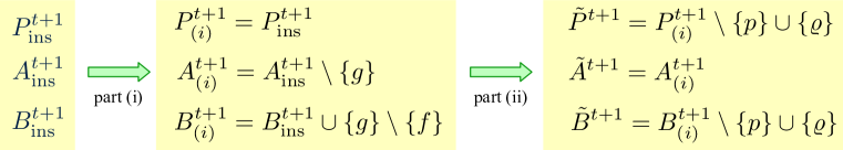
Figure 5.3: Changing ${{\mathcal{B}}}$ in two parts.

Claim 5.9.

Assume that $f={f^{\ast}}\neq\varrho$ or $g={g^{\ast}}\neq p$. Set ${{{B}}^{t+1}_{(i)}}={{{B}}^{t+1}_{{\mathrm{ins}}}}\cup{\left\{g\right\}}\setminus{\left\{f\right\}}$ is a feasible set of packets with respect to time $t+1$.

Proof.

The claim clearly holds if $d_{f}\leq d_{g}$, so for the rest of the proof we assume that $d_{g}<d_{f}$. Recall that, according to the assumptions of our Case L.$(\beta,\gamma]$.S.2, we have that either $\varrho\in{{{B}}^{t+1}_{{\mathrm{ins}}}}$ or ${{{A}}^{t+1}_{{\mathrm{ins}}}}(\beta,\gamma]\neq\emptyset$ holds.

It is sufficient to show that ${\textsf{pslack}}({{{B}}^{t+1}_{{\mathrm{ins}}}},\tau)\geq 1$ for any $\tau\in[d_{g},d_{f})$, as this will imply that $d_{f}\leq\textsf{nextts}({{{B}}^{t+1}_{{\mathrm{ins}}}},d_{g})$, which in turn implies the feasibility of ${{{B}}^{t+1}_{(i)}}$. We consider two cases.

First, assume that $\varrho\notin{{{B}}^{t+1}_{{\mathrm{ins}}}}$. This implies $f={f^{\ast}}$ and ${{{A}}^{t+1}_{{\mathrm{ins}}}}(\beta,\gamma]\neq\emptyset$, which means that $d_{g}\in(\beta,\gamma]$, no matter whether $g=p$ or $g={g^{\ast}}$. Then, for $\tau\in[d_{g},d_{f})$, Lemma 5.4(a) with $\zeta=\beta$ gives us

$${\textsf{pslack}}({{{B}}^{t+1}_{{\mathrm{ins}}}},\tau)\;\geq\;{\textsf{pslack}}({{{P}}^{t+1}_{{\mathrm{ins}}}},\tau)+|{{{A}}^{t+1}_{{\mathrm{ins}}}}(\beta,\tau]|\;\geq\;1,$$

since $g\in{{{A}}^{t+1}_{{\mathrm{ins}}}}(\beta,\tau]$ and ${\textsf{pslack}}({{{P}}^{t+1}_{{\mathrm{ins}}}},\tau)\geq 0$.

In the second case we have $\varrho\in{{{B}}^{t+1}_{{\mathrm{ins}}}}\setminus{{{P}}^{t+1}_{{\mathrm{ins}}}}$, so $f=\varrho$. We then have $g={g^{\ast}}$ (as we assume that $f\neq\varrho$ or $g\neq p$). For $\tau\in[d_{g},d_{f})$, we use Lemma 5.4(b) with $\zeta=\gamma$ to obtain

$${\textsf{pslack}}({{{B}}^{t+1}_{{\mathrm{ins}}}},\tau)\;\geq\;{\textsf{pslack}}({{{P}}^{t+1}_{{\mathrm{ins}}}},\tau)+|{{{B}}^{t+1}_{{\mathrm{ins}}}}(\tau,\gamma]\setminus{{{P}}^{t+1}_{{\mathrm{ins}}}}|\;\geq\;1,$$

where we use $f=\varrho\in{{{B}}^{t+1}_{{\mathrm{ins}}}}(\tau,\gamma]\setminus{{{P}}^{t+1}_{{\mathrm{ins}}}}$ in the second inequality. ∎

From the definitions of ${{{P}}^{t+1}_{(i)}}$, ${{{A}}^{t+1}_{(i)}}$, and ${{{B}}^{t+1}_{(i)}}$, and using Claim 5.9, invariants (InvA) and (InvB) hold for these three intermediate sets.

Before replacing $p$ by $\varrho$ in the optimal plan and in ${{\mathcal{B}}}$, we prove the following claim:

Claim 5.10.

Assume that $f={f^{\ast}}\neq\varrho$ or $g={g^{\ast}}\neq p$. If $d_{\varrho}<d_{p}$, then ${\textsf{pslack}}({{{B}}^{t+1}_{(i)}},\tau)\geq 1$ for any $\tau\in[d_{\varrho},d_{p})$.

Proof.

Let ${\hat{f}}$ be the earliest-deadline packet in ${{{B}}^{t+1}_{(i)}}(\beta,T]\setminus{{{P}}^{t+1}_{(i)}}$ and let ${\hat{g}}$ be the latest-deadline packet in ${{{A}}^{t+1}_{(i)}}[t+1,\gamma]$. These definitions are similar to the definitions of ${f^{\ast}}$ and ${g^{\ast}}$, but they are not equivalent because in part (i) we could have removed ${f^{\ast}}$ from ${{\mathcal{B}}}$ and ${g^{\ast}}$ from ${{\mathcal{A}}}$. For this reason, packets ${\hat{f}}$ and ${\hat{g}}$ may not actually exist, in which case, abusing notation, we will introduce artificial notations for their deadlines: if ${\hat{f}}$ does not exist, we let $d_{\hat{f}}=T$ and, similarly, if ${\hat{g}}$ does not exist, we let $d_{\hat{g}}=t+1$. We now observe that

$${\textsf{pslack}}({{{B}}^{t+1}_{(i)}},\tau)\geq{\textsf{pslack}}({{{P}}^{t+1}_{(i)}},\tau)\geq 1\quad\textrm{for}\;\tau\in(\beta,\min(d_{\hat{f}},\gamma))\cup[\max(d_{\hat{g}},\beta+1),\gamma).$$ (5.33)

Indeed, the first inequality follows from Lemma 5.4, which we can apply here because both invariants (InvA) and (InvB) are true for ${{{P}}^{t+1}_{(i)}}$, ${{{A}}^{t+1}_{(i)}}$, and ${{{B}}^{t+1}_{(i)}}$. Specifically, apply Lemma 5.4(a) with $\zeta=\beta$, obtaining the first inequality for $\tau\in(\beta,d_{\hat{f}})$, and Lemma 5.4(b) with $\zeta=\gamma$, to obtain the first inequality for $\tau\in(d_{\hat{g}},\gamma)$. To justify the second inequality in (5.33), note that, as $(\beta,\gamma]$ is a segment of ${{{P}}^{t+1}_{(i)}}={{{P}}^{t+1}_{{\mathrm{ins}}}}$, we have ${\textsf{pslack}}({{{P}}^{t+1}_{(i)}},\tau)\geq 1$ for $\tau\in(\beta,\gamma)$.

Since $[d_{\varrho},d_{p})\subseteq(\beta,\gamma)$, inequality (5.33) directly implies Claim 5.10 when $d_{\hat{f}}\geq\gamma$ or $d_{\hat{g}}\leq\beta$. Therefore, for the rest of the argument, we will assume that $d_{\hat{f}}<\gamma$ and $d_{\hat{g}}>\beta$.

Next, observe that, since ${{{B}}^{t+1}_{(i)}}$ is obtained from ${{{B}}^{t+1}_{{\mathrm{ins}}}}$ by replacing $f$ by $g$, we have

$${\textsf{pslack}}({{{B}}^{t+1}_{(i)}},\tau)={\textsf{pslack}}({{{B}}^{t+1}_{{\mathrm{ins}}}},\tau)+1\geq 1\quad\textrm{for}\;\tau\in[d_{f},d_{g}),$$ (5.34)

where the inequality follows from the feasibility of ${{{B}}^{t+1}_{{\mathrm{ins}}}}$. (It is possible that $d_{g}\leq d_{f}$, in which case this interval is empty.)

From these two observations, (5.33) and (5.34), it is now sufficient to show that

$$[d_{\varrho},d_{p})\;\subseteq\;(\beta,d_{\hat{f}})\cup[d_{f},d_{g})\cup[d_{\hat{g}},\gamma).$$ (5.35)

Note that $d_{\hat{g}}\leq d_{g^{\ast}}$ and $d_{\hat{f}}\geq d_{f^{\ast}}$, by the definitions of these packets and of ${{{B}}^{t+1}_{(i)}}$ and ${{{A}}^{t+1}_{(i)}}$ (note that $g$ is not a candidate for ${\hat{f}}$ as $g\in{{{P}}^{t+1}_{(i)}}$). Now we consider three cases.

If $f=\varrho$, then it holds that $g={g^{\ast}}$ by the claim’s assumption, and interval $[d_{\varrho},d_{p})$ is covered by $[d_{f},d_{g})=[d_{\varrho},d_{g^{\ast}})$ and $[d_{\hat{g}},\gamma)$, because $d_{\hat{g}}\leq d_{g^{\ast}}$ and $d_{p}\leq\gamma$.

Similarly, if $g=p$, then we have $f={f^{\ast}}$, and interval $[d_{\varrho},d_{p})$ is covered by $[d_{f},d_{g})=[d_{f^{\ast}},d_{p})$ and $(\beta,d_{\hat{f}})$, because $d_{\hat{f}}\geq d_{f^{\ast}}$.

The last case is when $f={f^{\ast}}$ and $g={g^{\ast}}$. Then interval $[d_{\varrho},d_{p})\subseteq(\beta,\gamma)$ is covered by $(\beta,d_{f^{\ast}})\cup[d_{f^{\ast}},d_{g^{\ast}})\cup[d_{g^{\ast}},\gamma)$, which implies (5.35) because $d_{\hat{f}}\geq d_{f^{\ast}}$ and $d_{\hat{g}}\leq d_{g^{\ast}}$. ∎

Finally, we show that the new backup plan ${\widetilde{{B}}^{t+1}}={{{B}}^{t+1}_{(i)}}\setminus{\left\{p\right\}}\cup{\left\{\varrho\right\}}$ is feasible. If $d_{\varrho}\geq d_{p}$, then the feasibility of ${{\mathcal{B}}}$ is clearly preserved after replacing $p$ by $\varrho$. Otherwise, $d_{\varrho}<d_{p}$, and for $\tau\in[d_{\varrho},d_{p})$ we have ${\textsf{pslack}}({\widetilde{{B}}^{t+1}},\tau)={\textsf{pslack}}({{{B}}^{t+1}_{(i)}},\tau)-1\geq 0$ by Claim 5.10, while ${\textsf{pslack}}({\widetilde{{B}}^{t+1}},\tau)={\textsf{pslack}}({{{B}}^{t+1}_{(i)}},\tau)\geq 0$ for $\tau\notin[d_{\varrho},d_{p})$ by Claim 5.9. Hence, invariant (InvB) holds after the step.

5.5.6 Processing $(\beta,\gamma]$ in an Iterated Leap Step

Here we address the last (and by far most involved) part of our argument, namely the analysis of an iterated leap step. As a reminder, this step occurs when $k\geq 1$ in the algorithm, or, equivalently, when $d_{\varrho}$ is in a later segment of ${{{P}}^{t}}$ than $d_{p}$. The initial comments in Section 5.5.5 apply here as well. To recap: We assume that ${{\mathcal{A}}}$ and ${{\mathcal{B}}}$ have already been modified as described in Sections 5.5.1 (the adversary step) and 5.5.4 (processing segment $[t,\alpha]$). In particular, the time step has already been incremented to $t+1$ and the current snapshots of ${{{\mathcal{P}}}}$, ${{{\mathcal{B}}}}$ and ${{{\mathcal{A}}}}$ are denoted ${{{P}}^{t+1}_{{\mathrm{ins}}}}$, ${{{B}}^{t+1}_{{\mathrm{ins}}}}$ and ${{{A}}^{t+1}_{{\mathrm{ins}}}}$, respectively. Recall that ${{{P}}^{t+1}_{{\mathrm{ins}}}}={{{P}}^{t}}\setminus{\left\{{\ell}\right\}}$. We assume that both invariants (InvA) and (InvB) hold for these sets (with respect to time step $t+1$).

As before, $\beta=\textsf{prevts}^{t}(d_{p})$ and $\gamma=\textsf{nextts}^{t}(d_{\varrho})$. As this is an iterated leap step, we have $d_{\varrho}>\textsf{nextts}^{t}(d_{p})$, so the interval $(\beta,\gamma]$ of ${{{P}}^{t+1}_{{\mathrm{ins}}}}$ is a union of two or more consecutive segments of ${{{P}}^{t+1}_{{\mathrm{ins}}}}$. (The content of this interval is identical to the same interval in ${{{P}}^{t}}$; in fact, ${{{P}}^{t+1}_{{\mathrm{ins}}}}$ and ${{{P}}^{t}}$ are identical starting right after $\alpha=\textsf{nextts}^{t}(t)$, the first tight slot of ${{{P}}^{t}}$.) Let $h_{0}=p,h_{1},\dots,h_{k}$ be the packets from Algorithm PlanM (line 9) and let $h_{k+1}=\varrho$. All packets $h_{0},h_{1},\dots,h_{k}$ are in different segments of ${{{P}}^{t+1}_{{\mathrm{ins}}}}$, not necessarily consecutive, while $h_{k+1}=\varrho$ has deadline in the same segment as $h_{k}$, but $\varrho\notin{{{P}}^{t+1}_{{\mathrm{ins}}}}$. The deadlines and weights of packets $\varrho$ and $h_{1},\dots,h_{k}$ are still unchanged before processing $(\beta,\gamma]$ (that is, they are the same as in step $t$).

We need to estimate the potential change due to weight increases and the changes triggered by the replacement of $p$ by $\varrho$ and by the “shifting” of $h_{i}$’s. We also need to prove key inequality (5.24) and that invariants (InvA) and (InvB) hold after the step.

The overall structure of the argument in this case is similar to Case L.$(\beta,\gamma]$.S (simple leap step), with the analysis split according to whether changes in ${{\mathcal{A}}}$ are needed (Case L.$(\beta,\gamma]$.I.2) or not (Case L.$(\beta,\gamma]$.I.1). In Case L.$(\beta,\gamma]$.I.2, the analysis will be divided into several stages corresponding to processing of different groups of segments.

For $i=0,\dots,k$, let $\mu_{i}={\textsf{minwt}}({{{P}}^{t}},d^{t}_{h_{i}})$; note that $w^{t}_{\ell}\geq\mu_{0}\geq\mu_{1}\geq\dots\geq\mu_{k}={\textsf{minwt}}({{{P}}^{t}},d_{\varrho})$ and the algorithm ensures that $w^{t+1}_{h_{i}}\geq\mu_{i-1}$ for $i=1,\dots,k+1$. In both cases below, we use the following simple bound on the change of weights of $h_{i}$’s.

Lemma 5.11.

For any $1\leq a^{\prime}\leq b^{\prime}\leq k$, let $\Delta^{t}w({h_{a^{\prime}}},\dots,{h_{b^{\prime}}})$ be the total amount by which the algorithm increases the weights of packets $h_{a^{\prime}},\dots,h_{b^{\prime}}$ in step $t$. Suppose that there exists $i\in[a^{\prime},b^{\prime}]$ such that $w^{t}_{h_{i}}<\mu_{i-1}$, i.e., the algorithm increases the weight of $h_{i}$ in Line 11 (and thus $\Delta^{t}w({h_{a^{\prime}}},\dots,{h_{b^{\prime}}})>0$). Then $\Delta^{t}w({h_{a^{\prime}}},\dots,{h_{b^{\prime}}})\leq\mu_{a^{\prime}-1}-w^{t}_{h_{b^{\prime}}}$.

Proof.

Let $c\in[a^{\prime},b^{\prime}]$ be the maximum index such that $w^{t}_{h_{c}}<\mu_{c-1}$; such $c$ exists by the assumption of the lemma. We show the claim as follows:

$$\Delta^{t}w({h_{a^{\prime}}},\dots,{h_{b^{\prime}}}) =\sum_{i=a^{\prime}}^{c}\max(\mu_{i-1}-w^{t}_{h_{i}},0)$$

$$\leq\sum_{i=a^{\prime}}^{c-1}\max(\mu_{i-1}-\mu_{i},0)+\max(\mu_{c-1}-w^{t}_{h_{c}},0)$$ (5.36)

$$=\sum_{i=a^{\prime}}^{c-1}(\mu_{i-1}-\mu_{i})+\mu_{c-1}-w^{t}_{h_{c}}$$ (5.37)

$$=\mu_{a^{\prime}-1}-w^{t}_{h_{c}}$$

$$\leq\mu_{a^{\prime}-1}-w^{t}_{h_{b^{\prime}}}\,,$$ (5.38)

where inequality (5.36) follows from $w^{t}_{h_{i}}\geq\mu_{i}$, equality (5.37) from $\mu_{i-1}\geq\mu_{i}$ and from $\mu_{c-1}>w^{t}_{h_{c}}$ (by the choice of $c$), and inequality (5.38) from $w^{t}_{h_{c}}\geq w^{t}_{h_{b^{\prime}}}$ by Lemma B.1(b) and $c\leq b^{\prime}$. ∎

Case L.$(\beta,\gamma]$.I.1: $\varrho\notin{{{B}}^{t+1}_{{\mathrm{ins}}}}$ and ${{{A}}^{t+1}_{{\mathrm{ins}}}}(\beta,\gamma]=\emptyset$. In this case, we do not make any changes in ${{\mathcal{A}}}$, i.e. ${\widetilde{{A}}^{t+1}}={{{A}}^{t+1}_{{\mathrm{ins}}}}$. From the case condition, $p=h_{0},h_{1},...,h_{k}\notin{{{A}}^{t+1}_{{\mathrm{ins}}}}$, because each $h_{i}$ is in ${{{P}}^{t+1}_{{\mathrm{ins}}}}(\beta,\gamma]$. It follows that ${{\mathcal{A}}}$ is indeed not affected by the decrease of the deadlines of $h_{i}$’s. Thus invariant (InvA) holds. Note that $\varrho\notin{{{A}}^{t+1}_{{\mathrm{ins}}}}$ by invariant (InvA). From the case condition and $p\in{{{P}}^{t+1}_{{\mathrm{ins}}}}(\beta,\gamma]$, we have $p\notin{{{A}}^{t+1}_{{\mathrm{ins}}}}$; therefore $p\in{{{B}}^{t+1}_{{\mathrm{ins}}}}$ by invariant (InvB)(ii). This means that in order to preserve invariant (InvB)(ii) we need to remove $p$ from ${{\mathcal{B}}}$ and add $\varrho$ to it. Thus we set ${\widetilde{{B}}^{t+1}}={{{B}}^{t+1}_{{\mathrm{ins}}}}\setminus{\left\{p\right\}}\cup{\left\{\varrho\right\}}$.

Deriving inequality (5.24). To prove this inequality, we first show that

$$\Delta^{t}w({h_{1}},\dots,{h_{k}})\;\leq\;\mu_{0}-\mu_{k}.$$ (5.39)

(The weight increase $\Delta^{t}w({h_{1}},\dots,{h_{k}})$ was defined in Lemma 5.11.) Indeed, if there is no $i\in[1,k]$ such that $w^{t}_{h_{i}}<\mu_{i-1}$, then $\Delta^{t}w({h_{1}},\dots,{h_{k}})=0\leq\mu_{0}-\mu_{k}$ as $\mu_{0}\geq\mu_{k}$. Otherwise, we use Lemma 5.11 with $a^{\prime}=1$ and $b^{\prime}=k$ to get $\Delta^{t}w({h_{1}},\dots,{h_{k}})\leq\mu_{0}-w^{t}_{h_{k}}\leq\mu_{0}-\mu_{k}$, where the last inequality follows from $w^{t}_{h_{k}}\geq\mu_{k}$.

In this case, the terms on the left-hand side of inequality (5.24) are

$$\Delta_{(\beta,\gamma]}\Psi\; =\;{\textstyle{\frac{1}{\phi}}}{\,}\big{(}-w^{t}_{p}+w^{t+1}_{\varrho}+\Delta^{t}w({h_{1}},\dots,{h_{k}})\big{)}$$

$$\Delta^{t}{w}\; =\;w^{t+1}_{\varrho}-w^{t}_{\varrho}+\Delta^{t}w({h_{1}},\dots,{h_{k}})$$

$$\textsf{advcredit}^{t}_{(\beta,\gamma]}\; =\;0$$

The equation for $\Delta_{(\beta,\gamma]}\Psi$ is true because all packets $h_{1},...,h_{k}$ are both in ${{{P}}^{t+1}_{{\mathrm{ins}}}}$ and in ${\widetilde{{P}}^{t+1}}$, by Lemma B.1(a), and none of them is in ${{{A}}^{t+1}_{{\mathrm{ins}}}}={\widetilde{{A}}^{t+1}}$, so we keep all of them in ${{\mathcal{B}}}$ to preserve invariant (InvB)(ii). The last equation holds because we have not changed the adversary stash. Plugging in these formulas, taking into account that $w_{\varrho}^{t+1}=\mu_{k}$, and using inequality (5.39), we can obtain inequality (5.24) with an easy calculation:

$$\Delta_{(\beta,\gamma]}\Psi -\phi{\,}(\Delta^{t}{w})-\textsf{advcredit}^{t}_{(\beta,\gamma]}$$

$$=\;{\textstyle{\frac{1}{\phi}}}{\,}(-w^{t}_{p}+w^{t+1}_{\varrho}+\Delta^{t}w({h_{1}},\dots,{h_{k}}))$$

$$\qquad\qquad-\phi{\,}(w^{t+1}_{\varrho}-w^{t}_{\varrho}+\Delta^{t}w({h_{1}},\dots,{h_{k}}))-0$$

$$=\;-{\textstyle{\frac{1}{\phi}}}{\,}w^{t}_{p}-\mu_{k}+\phi{\,}w^{t}_{\varrho}-\Delta^{t}w({h_{1}},\dots,{h_{k}})$$

$$\geq\;-{\textstyle{\frac{1}{\phi}}}{\,}w^{t}_{p}-\mu_{k}+\phi{\,}w^{t}_{\varrho}-(\mu_{0}-\mu_{k})$$

$$=\;-{\textstyle{\frac{1}{\phi}}}{\,}w^{t}_{p}+\phi w^{t}_{\varrho}-\mu_{0}$$

$$\geq\;-{\textstyle{\frac{1}{\phi}}}{\,}w^{t}_{p}+\phi{\,}w^{t}_{\varrho}-({\textstyle{\frac{1}{\phi^{2}}}}{\,}w_{p}^{t}+{\textstyle{\frac{1}{\phi}}}{\,}w_{\varrho}^{t})$$ (5.40)

$$=\;-w^{t}_{p}+w^{t}_{\varrho}\,,$$

where inequality (5.40) follows from ${\mu_{0}}={\textsf{minwt}}({{{P}}^{t}},d_{p})\leq{\textstyle{\frac{1}{\phi^{2}}}}{\,}w_{p}^{t}+{\textstyle{\frac{1}{\phi}}}{\,}w_{\varrho}^{t}$, which is inequality (5.26) with $\tau=d_{p}$.

Preserving invariant (InvB). That invariant (InvB)(ii) is preserved follows immediately from the definitions of ${\widetilde{{P}}^{t+1}}$, ${\widetilde{{A}}^{t+1}}$, and ${\widetilde{{B}}^{t+1}}$. Next, we show invariant (InvB)(i), that is the feasibility of ${\widetilde{{B}}^{t+1}}$, and we split the argument into two parts. First, we show that the invariant holds for the intermediate backup plan resulting from replacing $p$ by $\varrho$, and then later we show that modifying the deadlines of the $h_{i}$’s preserves the invariant as well.

So consider an intermediate plan ${{{P}}^{t+1}_{(i)}}={{{P}}^{t+1}_{{\mathrm{ins}}}}\setminus{\left\{p\right\}}\cup{\left\{\varrho\right\}}$ and backup plan ${{{B}}^{t+1}_{(i)}}={{{B}}^{t+1}_{{\mathrm{ins}}}}\setminus{\left\{p\right\}}\cup{\left\{\varrho\right\}}$, both with respect to time $t+1$ but with the deadlines of packets $h_{1},h_{2},...,h_{k}$ still unchanged. Since this is an iterated leap step, we have that $d_{\varrho}>d_{p}$, so replacing $p$ by $\varrho$ in ${{\mathcal{B}}}$ preserves feasibility. Therefore ${{{B}}^{t+1}_{(i)}}$ is feasible.

Now, we consider ${\widetilde{{B}}^{t+1}}$, that is the backup plan at step $t+1$, which is obtained from ${{{B}}^{t+1}_{(i)}}$ by decreasing the deadlines of $h_{i}$’s, as in the algorithm. As slots outside $(\beta,\gamma)$ are not affected, we have ${\textsf{pslack}}({\widetilde{{B}}^{t+1}},\tau)={\textsf{pslack}}({{{B}}^{t+1}_{(i)}},\tau)\geq 0$ for $\tau\notin(\beta,\gamma)$. So it remains to consider slots $\tau\in(\beta,\gamma)$.

Recall that packets $h_{1},\dots,h_{k}$ belong to both ${{{B}}^{t+1}_{{\mathrm{ins}}}}$ and ${\widetilde{{B}}^{t+1}}$. We also have that ${\textsf{pslack}}({{{P}}^{t+1}_{(i)}},\tau)\geq 1$ for any $\tau\in(\beta,\gamma)$, which holds as replacing $p$ by $\varrho$ merges all segments between $\beta=\textsf{prevts}^{t}(d_{p})$ and $\gamma=\textsf{nextts}^{t}(d_{\varrho})$. Since ${{{A}}^{t+1}_{(i)}}(\beta,\gamma]={{{A}}^{t+1}_{{\mathrm{ins}}}}(\beta,\gamma]=\emptyset$, Lemma 5.4(b) with $\zeta=\gamma$ gives us that for any $\tau\in(\beta,\gamma)$,

$${\textsf{pslack}}({{{B}}^{t+1}_{(i)}},\tau)\geq{\textsf{pslack}}({{{P}}^{t+1}_{(i)}},\tau)\geq 1\,.$$ (5.41)

Next, we claim that for $\tau\in(\beta,\gamma)$,

$${\textsf{pslack}}({\widetilde{{B}}^{t+1}},\tau)\geq{\textsf{pslack}}({{{B}}^{t+1}_{(i)}},\tau)-1\,.$$ (5.42)

To justify this inequality, we observe that $d^{t+1}_{h_{i}}=\tau_{i-1}\geq d^{t}_{h_{i-1}}$ for $i=1,\dots,k$, which gives us that intervals $[d^{t+1}_{h_{i}},d^{t}_{h_{i}})\subset(\beta,\gamma)$ are disjoint. This implies in turn that, for $\tau\in(\beta,\gamma)$, decreasing the deadlines of all $h_{i}$’s can decrease ${\textsf{pslack}}({\mathcal{B}},\tau)$ at most by one, which yields inequality (5.42).

Inequalities (5.41) and (5.42) yield ${\textsf{pslack}}({\widetilde{{B}}^{t+1}},\tau)\geq{\textsf{pslack}}({{{B}}^{t+1}_{(i)}},\tau)-1\geq 0$ for $\tau\in(\beta,\gamma)$, completing the proof that ${\widetilde{{B}}^{t+1}}$ satisfies invariant (InvB)(i).

Case L.$(\beta,\gamma]$.I.2: $\varrho\in{{{B}}^{t+1}_{{\mathrm{ins}}}}$ or ${{{A}}^{t+1}_{{\mathrm{ins}}}}(\beta,\gamma]\neq\emptyset$. In this case, both sets ${{\mathcal{A}}}$ and ${{\mathcal{B}}}$ will be changed. We focus on the segments of ${{{P}}^{t+1}_{{\mathrm{ins}}}}$ which contain the packets $h_{0}=p,h_{1},...,h_{k}$. These are the segments of the current optimal plan that are modified by the algorithm when $p$ is transmitted. Specifically, for $i=0,\dots,k$, let $S_{i}$ be the segment of ${{{P}}^{t+1}_{{\mathrm{ins}}}}$ that ends at $\tau_{i}=\textsf{nextts}^{t}(d^{t}_{h_{i}})$, that is the segment containing $d^{t}_{h_{i}}$. (See Figure 4.1.) Recall that $\textsf{prevts}^{t}(d_{p})=\beta$, $\tau_{k}=\gamma$, and that we defined $h_{k+1}=\varrho$. We first organize segments $S_{i}$ into groups and then split the sequence of changes in this case into stages, having one stage for each group.

Groups.

We start by defining a packet $g\in{{{A}}^{t+1}_{{\mathrm{ins}}}}$. Let ${g^{\ast}}$ be the latest-deadline packet in ${{{A}}^{t+1}_{{\mathrm{ins}}}}[t+1,\gamma]$. Observe that packet ${g^{\ast}}$ is well-defined. This is trivially true if the second part of the case condition holds, while in the case when $\varrho\in{{{B}}^{t+1}_{{\mathrm{ins}}}}\setminus{{{P}}^{t+1}_{{\mathrm{ins}}}}$, we use Observation 5.2(b) with $\eta=\gamma$ to get that ${{{A}}^{t+1}_{{\mathrm{ins}}}}[t+1,\gamma]\neq\emptyset$. (It is possible that $d_{{g^{\ast}}}\leq\beta$ in the second case.)

We now define $g$ as follows: If $d^{t}_{{g^{\ast}}}$ is in a segment $S_{i}$ for which $h_{i}\in{{{A}}^{t+1}_{{\mathrm{ins}}}}$, then let $g=h_{i}$; otherwise let $g={g^{\ast}}$. Observe that, in particular, if $h_{k}\in{{{A}}^{t+1}_{{\mathrm{ins}}}}$ then $g=h_{k}$.

We will process segments $S_{i}$ in groups, where each group is specified by some non-empty interval of indices $[a,b]\subseteq{\left\{0,\dots,k\right\}}$ of segments $S_{i}$. We will denote such a group by ${\langle a,b\rangle}$ (to avoid confusion with the notation for segments and time intervals). These intervals will be chosen so that they partition the set of all indices ${\left\{0,\dots,k\right\}}$. Roughly, we have a group for each $h_{i}\in{{{A}}^{t+1}_{{\mathrm{ins}}}}$ (that needs to be replaced in or removed from ${{\mathcal{A}}}$ because its deadline needs to be decreased), a special last group, and possibly a special group at the beginning. Let $i_{1}<i_{2}<\cdots<i_{l}$ be the indices of those packets $h_{0}=p,h_{1},...,h_{k}$ that are in ${{{A}}^{t+1}_{{\mathrm{ins}}}}$. Note that, if $l>0$, then $d^{t}_{g}\in[d^{t}(h_{i_{l}}),\gamma]$, because $h_{i_{l}}\in{{{A}}^{t+1}_{{\mathrm{ins}}}}$ is a candidate for ${g^{\ast}}$. In particular, since $g\in{{{A}}^{t+1}_{{\mathrm{ins}}}}$, we have that $g\notin{\left\{h_{0},...,h_{k}\right\}}\setminus{\left\{h_{i_{l}}\right\}}$; that is, among all packets $h_{0},...,h_{k}$, $g$ may be possibly equal only to $h_{i_{l}}$. The definition of these groups depends on whether some packet $h_{i}$ is in ${{{A}}^{t+1}_{{\mathrm{ins}}}}$ (that is $l>0$) or none of them is in ${{{A}}^{t+1}_{{\mathrm{ins}}}}$ (that is $l=0$):

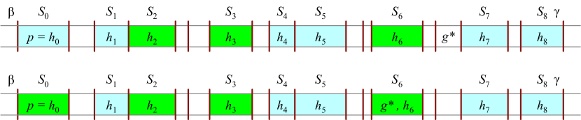
Figure 5.4: Two examples that illustrate assigning segments into groups. In both examples we have $k=8$. Segments are separated by vertical bars. Segments $S_{i}$ are colored (shaded). Green (or dark shaded) segments $S_{i}$ are those for which packet $h_{i}$ is in ${{{A}}^{t+1}_{{\mathrm{ins}}}}$. In the first example, we have $l=3$, $(i_{1},i_{2},i_{3})=(2,3,6)$, $g={g^{\ast}}$ (as ${g^{\ast}}$ is not in $S_{i}$ for any $i$), and ${{\tilde{a}}}=7$. We have 5 groups: the initial group ${\langle 0,1\rangle}$, middle groups ${\langle 2,2\rangle}$, ${\langle 3,5\rangle}$, and ${\langle 6,6\rangle}$, and the terminal group ${\langle 7,8\rangle}$. In the second example we have $l=4$, $(i_{1},i_{2},i_{3},i_{4})=(0,2,3,6)$, and $g=h_{6}$ (because ${g^{\ast}}$ is in $S_{6}$ and $h_{6}$ is in ${{{A}}^{t+1}_{{\mathrm{ins}}}}$). Since $i_{1}=0$ there is no initial group. We have 4 groups: middle groups ${\langle 0,1\rangle}$, ${\langle 2,2\rangle}$, ${\langle 3,5\rangle}$, and the terminal group ${\langle 6,8\rangle}$.

Case $l>0$: If $l>1$, then for each $c=1,\dots,l-1$, the interval ${\langle i_{c},i_{c+1}-1\rangle}$ is a middle group. If $i_{1}>0$ (meaning that $h_{0}=p\not\in{{{A}}^{t+1}_{{\mathrm{ins}}}}$), then there is a special initial group ${\langle 0,i_{1}-1\rangle}$. If $i_{1}=0$ then there is no initial group. Next, we assign the indices in $[i_{l},k]$ to one or two groups and define index ${{\tilde{a}}}$. If $g=h_{i_{l}}$ (in particular, if $i_{l}=k$), then ${\langle i_{l},k\rangle}$ is the terminal group and we let ${{\tilde{a}}}=i_{l}$. Otherwise, $g\neq h_{i_{l}}$ and we let ${{\tilde{a}}}$ be the smallest index in $0,...,k$ for which $\tau_{{\tilde{a}}}\geq d^{t}_{g}$. The assumption that $g\neq h_{i_{l}}$ implies that ${{\tilde{a}}}>i_{l}$. Then ${\langle{{\tilde{a}}},k\rangle}$ is the terminal group and ${\langle i_{l},{{\tilde{a}}}-1\rangle}$ is a new middle group. (See Figure 5.4 for two examples that illustrate the case when $l>0$.)

Case $l=0$: We define one or two groups only. There is the terminal group ${\langle{{\tilde{a}}},k\rangle}$, where ${{\tilde{a}}}$ is again the smallest index in $0,...,k$ with $\tau_{{\tilde{a}}}\geq d^{t}_{g}$. If ${{\tilde{a}}}>0$, we also have the initial group ${\langle 0,{{\tilde{a}}}-1\rangle}$ .

Observe that we always define ${{\tilde{a}}}$ so that ${\langle{{\tilde{a}}},k\rangle}$ is the terminal group. We further define index ${{\tilde{b}}}$ so that the first group is ${\langle 0,{{\tilde{b}}}\rangle}$; for example, if $l>0$ and $i_{1}>0$, then ${{\tilde{b}}}=i_{1}-1$. Note that in almost every group ${\langle a,b\rangle}$ packet $h_{a}$ is in ${{{A}}^{t+1}_{{\mathrm{ins}}}}$; the only two possible exceptions are (i) the initial group, and (ii) the terminal group in case when either $l=0$ or $l\geq 1$ and ${{\tilde{a}}}\neq i_{l}$. On the other hand, for any group ${\langle a,b\rangle}$ packets $h_{a+1},\dots,h_{b}$ are never in ${{{A}}^{t+1}_{{\mathrm{ins}}}}$ and thus these packets are in ${{{B}}^{t+1}_{{\mathrm{ins}}}}$ by invariant (InvB)(ii).

Stages.

The changes implemented during the processing of interval $(\beta,\gamma]$ involve the replacement of $p$ by $\varrho$ in ${{\mathcal{P}}}$, weight increases of $\varrho$ and $h_{i}$’s, and deadline decreases of $h_{i}$’s, as described in the algorithm. These changes will also trigger changes of ${{\mathcal{B}}}$ and ${{\mathcal{A}}}$ necessary to preserve the invariants. We will organize all these changes (of ${{\mathcal{P}}}$, ${{\mathcal{B}}}$, ${{\mathcal{A}}}$, and the instance itself) into a sequence of stages, with one stage for each group ${\langle a,b\rangle}$. The stages will be implemented in the reverse order of the groups, that is, starting from the stage for the terminal group (which is defined in all cases), continuing with middle groups in the reverse order of their indices, and ending by the group containing index $0$, which may be of any type.

To understand better the partition into stages, as described below, it helps to think of the substitution of $p$ by $\varrho=h_{k+1}$ in the optimal plan as a chain of substitutions: first replace $h_{k}$ by $\varrho$, then replace $h_{k-1}$ by $h_{k}$, and so on, and eventually replace $p=h_{0}$ by $h_{1}$. In our process here, rather than processing these substitutions individually, we process the substitutions within each group ${\langle a,b\rangle}$ simultaneously as one stage, in which $h_{a}$ is replaced by $h_{b+1}$. (See Figure 5.5 for illustration.)

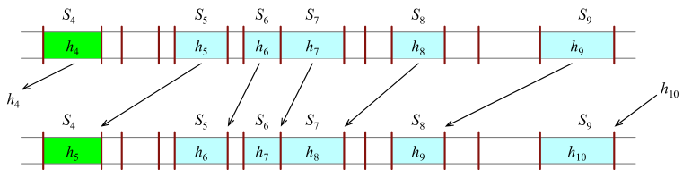
Figure 5.5: An illustration of the changes in ${{\mathcal{P}}}$ in the stage when a middle group ${\langle a,b\rangle}={\langle 4,9\rangle}$ is processed.

Formally, let ${\dot{{P}}^{t+1}_{{\langle a,b\rangle}}}$ be the snapshot of the intermediate plan ${{\mathcal{P}}}$ just before the stage for group ${\langle a,b\rangle}$ and let ${\ddot{{P}}^{t+1}_{{\langle a,b\rangle}}}$ be the snapshot of the intermediate plan ${{\mathcal{P}}}$ just after the stage for group ${\langle a,b\rangle}$. (We remark that ${\dot{{P}}^{t+1}_{{\langle a,b\rangle}}}$ is not necessarily an optimal plan. It is only meant to be an “intermediate plan” used to capture gradual changes in the optimal plan as stages are executed. It is, however, feasible and it will satisfy appropriate invariants.) Naturally, if ${\langle a,b\rangle}$ and ${\langle b+1,c\rangle}$ are two consecutive groups, then ${\ddot{{P}}^{t+1}_{{\langle b+1,c\rangle}}}={\dot{{P}}^{t+1}_{{\langle a,b\rangle}}}$. We adopt the same conventions for sets ${{\mathcal{B}}}$ and ${{\mathcal{A}}}$. In this notation (see Figure 5.6 for illustration):

• In the first stage, that corresponds to the terminal group ${\langle{{\tilde{a}}},k\rangle}$, we have ${\dot{{P}}^{t+1}_{{\langle{{\tilde{a}}},k\rangle}}}={{{P}}^{t+1}_{{\mathrm{ins}}}}$, ${\dot{{B}}^{t+1}_{{\langle{{\tilde{a}}},k\rangle}}}={{{B}}^{t+1}_{{\mathrm{ins}}}}$ and ${\dot{{A}}^{t+1}_{{\langle{{\tilde{a}}},k\rangle}}}={{{A}}^{t+1}_{{\mathrm{ins}}}}$. Note that in this stage, it holds that $h_{k+1}=\varrho\notin{\dot{{P}}^{t+1}_{{\langle{{\tilde{a}}},k\rangle}}}$.

• When describing the stage for each group ${\langle a,b\rangle}$, we assume that the changes in stages for groups ${\langle a^{\prime},b^{\prime}\rangle}$ with $a^{\prime}>b$ have already been implemented. As an invariant we will ensure that $h_{b+1}\notin{\dot{{P}}^{t+1}_{{\langle a,b\rangle}}}$ (for $b=k$, this holds by $h_{k+1}=\varrho\notin{\dot{{P}}^{t+1}_{{\langle{{\tilde{a}}},k\rangle}}}={{{P}}^{t+1}_{{\mathrm{ins}}}}$). In this stage, the plan changes from ${\dot{{P}}^{t+1}_{{\langle a,b\rangle}}}$ to ${\ddot{{P}}^{t+1}_{{\langle a,b\rangle}}}={\dot{{P}}^{t+1}_{{\langle a,b\rangle}}}\setminus{\left\{h_{a}\right\}}\cup{\left\{h_{b+1}\right\}}$, which will imply that $h_{a}\notin{\ddot{{P}}^{t+1}_{{\langle a,b\rangle}}}$ just after this stage is processed. Further, the weights and deadlines of packets $h_{a+1},...,h_{b+1}$ are adjusted according to the algorithm (for $b=k$, the deadline of $h_{k+1}=\varrho$ remains the same). This stage also involves changes in ${{\mathcal{A}}}$ and ${{\mathcal{B}}}$ triggered by the changes in ${{\mathcal{P}}}$ and by the adjustments of weights and deadlines. These changes will convert ${\dot{{B}}^{t+1}_{{\langle a,b\rangle}}}$ and ${\dot{{A}}^{t+1}_{{\langle a,b\rangle}}}$ to ${\ddot{{B}}^{t+1}_{{\langle a,b\rangle}}}$ and ${\ddot{{A}}^{t+1}_{{\langle a,b\rangle}}}$, respectively.

• After the last stage, corresponding to the first group ${\langle 0,{{\tilde{b}}}\rangle}$ (which could be an initial, middle, or terminal group), we have ${\ddot{{P}}^{t+1}_{{\langle 0,{{\tilde{b}}}\rangle}}}={\widetilde{{P}}^{t+1}}$, ${\ddot{{B}}^{t+1}_{{\langle 0,{{\tilde{b}}}\rangle}}}={\widetilde{{B}}^{t+1}}$, and ${\ddot{{A}}^{t+1}_{{\langle 0,{{\tilde{b}}}\rangle}}}={\widetilde{{A}}^{t+1}}$.

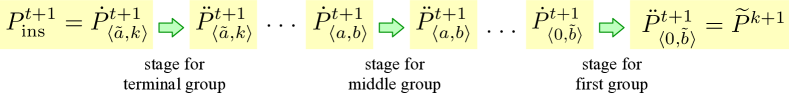
Figure 5.6: Notation for stages.

By the results of Section 5.5.4, invariants (InvA) and (InvB) hold for ${\dot{{P}}^{t+1}_{{\langle{{\tilde{a}}},k\rangle}}}$, ${\dot{{B}}^{t+1}_{{\langle{{\tilde{a}}},k\rangle}}}$, and ${\dot{{A}}^{t+1}_{{\langle{{\tilde{a}}},k\rangle}}}$. In the stage for each group ${\langle a,b\rangle}$, we will show that these invariants are preserved and that an appropriate bound on amortized profits holds. This will give us that inequality (5.24) holds when processing interval $(\beta,\gamma]$ and that invariants (InvA) and (InvB) hold afterwards, that is for sets ${\widetilde{{P}}^{t+1}}$, ${\widetilde{{B}}^{t+1}}$, and ${\widetilde{{A}}^{t+1}}$.

Note that the changes of ${{\mathcal{P}}}$ implemented by the algorithm in the stage for group ${\langle a,b\rangle}$ satisfy

$${\dot{{P}}^{t+1}_{{\langle a,b\rangle}}}\setminus{\dot{{P}}^{t+1}_{{\langle a,b\rangle}}}(\eta,\tau_{b}]={\ddot{{P}}^{t+1}_{{\langle a,b\rangle}}}\setminus{\ddot{{P}}^{t+1}_{{\langle a,b\rangle}}}(\eta,\tau_{b}]$$

for $\eta=\textsf{prevts}({\dot{{P}}^{t+1}_{{\langle a,b\rangle}}},d^{t}_{h_{a}})$, which is the “locality of changes” invariant (5.29) from Section 5.5.3. The ${\textsf{pslack}}({{\mathcal{P}}},\tau)$ values are actually affected only for $\tau\in[d^{t}_{h_{a}},\tau_{b})$. (We remark that changes of ${{\mathcal{P}}}$ involve packet $h_{b+1}$ with $d^{t}_{h_{b+1}}>\tau_{b}$ (if $b<k$), however, $h_{b+1}\notin{\dot{{P}}^{t+1}_{{\langle a,b\rangle}}}$ and we change the deadline of $h_{b+1}$ to $\tau_{b}$ during the stage for group ${\langle a,b\rangle}$.)

Finally, we will maintain the property that after the stage for each group ${\langle a,b\rangle}$, packet $h_{a}$ will not be in ${\ddot{{A}}^{t+1}_{{\langle a,b\rangle}}}$ — even though it may have been in ${{\mathcal{A}}}$ earlier. This is necessary for invariant (InvA), because $h_{a}\notin{\ddot{{P}}^{t+1}_{{\langle a,b\rangle}}}$. As also $\varrho=h_{k+1}\notin{\dot{{A}}^{t+1}_{{\langle{{\tilde{a}}},k\rangle}}}={{{A}}^{t+1}_{{\mathrm{ins}}}}$, this will give us that $h_{b+1}\notin{\dot{{A}}^{t+1}_{{\langle a,b\rangle}}}$ for any group ${\langle a,b\rangle}$. Recall that, importantly, packets $h_{a+1},\dots,h_{b}$ are also not in ${\dot{{A}}^{t+1}_{{\langle a,b\rangle}}}$.

Deriving inequality (5.24). We split the potential changes and the adversary credit for replacing packets in ${{\mathcal{A}}}$ among groups in a natural way. Let $\Delta_{{\langle a,b\rangle}}\Psi$ be the total change of the potential due to the modifications implemented in the stage for group ${\langle a,b\rangle}$, and let $\textsf{advcredit}^{t}_{{\langle a,b\rangle}}$ be the adversary adjustment credit for the changes of ${{\mathcal{A}}}$ implemented in the stage for group ${\langle a,b\rangle}$ (that is, for removing a packet or for replacing $h_{a}$ by a lighter packet). Recall that $\Delta^{t}w({h_{a+1}},\dots,{h_{b+1}})$ is the total amount by which the algorithm increases the weights of $h_{a+1},\dots,h_{b+1}$. Our goal is to prove for each group ${\langle a,b\rangle}$ that

$$\Delta_{{\langle a,b\rangle}}\Psi-\phi{\,}\Delta^{t}w({h_{a+1}},\dots,{h_{b+1}})-\textsf{advcredit}^{t}_{{\langle a,b\rangle}}\geq-w^{t}_{h_{a}}+w^{t}_{h_{b+1}}\,.$$ (5.43)

(Note that the right-hand side of (5.43) is negative, by Lemma B.1(b).)

It remains to observe that the sum of (5.43) over all groups gives us exactly the key inequality (5.24). Indeed, the right-hand sides sum to $-w^{t}_{h_{0}}+w^{t}_{h_{k+1}}=-w^{t}_{p}+w^{t}_{\varrho}$. Regarding the left-hand side of (5.43), $\Delta_{(\beta,\gamma]}\Psi$ equals the sum of $\Delta_{{\langle a,b\rangle}}\Psi$ over all groups ${\langle a,b\rangle}$, and similarly for $\Delta^{t}{w}$ and $\textsf{advcredit}^{t}_{(\beta,\gamma]}$. (Note that the increase of the weight of $\varrho=h_{k+1}$ is accounted for in inequality (5.43) for the terminal group ${\langle{{\tilde{a}}},k\rangle}$.)

Stage for the terminal group.

Let ${\langle{{\tilde{a}}},k\rangle}$ be the terminal group of segments. In this stage, we change plan ${{\mathcal{P}}}$ by removing $h_{{\tilde{a}}}$ and adding $\varrho$, we increase the weights of packets $h_{{{\tilde{a}}}+1},\dots,h_{k+1}=\varrho$, and we decrease the deadlines of packets $h_{{{\tilde{a}}}+1},\dots,h_{k}$. We thus have ${\ddot{{P}}^{t+1}_{{\langle{{\tilde{a}}},k\rangle}}}={\dot{{P}}^{t+1}_{{\langle{{\tilde{a}}},k\rangle}}}\setminus{\left\{h_{{\tilde{a}}}\right\}}\cup{\left\{\varrho\right\}}$.

Let ${f^{\ast}}$ be the earliest-deadline packet in ${\dot{{B}}^{t+1}_{{\langle{{\tilde{a}}},k\rangle}}}(\beta,{T}]\setminus{\dot{{P}}^{t+1}_{{\langle{{\tilde{a}}},k\rangle}}}$. We argue that packet ${f^{\ast}}$ is well-defined, which is trivially true if $\varrho\in{{{B}}^{t+1}_{{\mathrm{ins}}}}(\beta,{T}]={\dot{{B}}^{t+1}_{{\langle{{\tilde{a}}},k\rangle}}}(\beta,{T}]$. Otherwise, ${{{A}}^{t+1}_{{\mathrm{ins}}}}(\beta,\gamma]={\dot{{A}}^{t+1}_{{\langle{{\tilde{a}}},k\rangle}}}(\beta,\gamma]\neq\emptyset$ and then Observation 5.2(a) with $\eta=\beta$ implies that ${\dot{{B}}^{t+1}_{{\langle{{\tilde{a}}},k\rangle}}}(\beta,{T}]\setminus{\dot{{P}}^{t+1}_{{\langle{{\tilde{a}}},k\rangle}}}\neq\emptyset$. (Possibly, $d_{f^{\ast}}>\gamma$ in the second case.)

We then define a packet $f\in{\dot{{B}}^{t+1}_{{\langle{{\tilde{a}}},k\rangle}}}\setminus{\dot{{P}}^{t+1}_{{\langle{{\tilde{a}}},k\rangle}}}$, letting $f=\varrho$ if $\varrho\in{\dot{{B}}^{t+1}_{{\langle{{\tilde{a}}},k\rangle}}}$, and $f={f^{\ast}}$ otherwise.

Next, we modify sets ${{\mathcal{A}}}$ and ${{\mathcal{B}}}$. We remove $g$ from ${{\mathcal{A}}}$, i.e., ${\ddot{{A}}^{t+1}_{{\langle{{\tilde{a}}},k\rangle}}}={\dot{{A}}^{t+1}_{{\langle{{\tilde{a}}},k\rangle}}}\setminus{\left\{g\right\}}$. This ensures that invariant (InvA) is preserved, because $h_{{\tilde{a}}}\notin{\ddot{{A}}^{t+1}_{{\langle{{\tilde{a}}},k\rangle}}}$ and none of packets $h_{{{\tilde{a}}}+1},\dots,h_{k}$ is in ${\ddot{{A}}^{t+1}_{{\langle{{\tilde{a}}},k\rangle}}}$ (by the definition of groups), thus the decrease of their deadlines, implemented in this stage, does not affect ${{\mathcal{A}}}$.

Regarding ${{\mathcal{B}}}$, note that $\varrho\in{\ddot{{P}}^{t+1}_{{\langle{{\tilde{a}}},k\rangle}}}\setminus{\ddot{{A}}^{t+1}_{{\langle{{\tilde{a}}},k\rangle}}}$, so we need to include $\varrho$ in ${\ddot{{B}}^{t+1}_{{\langle{{\tilde{a}}},k\rangle}}}$ to preserve invariant (InvB)(ii). Hence, we let ${\ddot{{B}}^{t+1}_{{\langle{{\tilde{a}}},k\rangle}}}={{{B}}^{t+1}_{{\mathrm{ins}}}}\cup{\left\{g\right\}}\setminus{\left\{f,h_{{\tilde{a}}}\right\}}\cup{\left\{\varrho\right\}}$; this definition applies no matter whether $g=h_{{\tilde{a}}}$ or $g={g^{\ast}}$ and whether $f=\varrho$ or $f={f^{\ast}}$.

Deriving (5.43) for the terminal group. Apart from the changes in the paragraph above, the algorithm changes the weights of packets $h_{{{\tilde{a}}}+1},\dots,h_{k+1}=\varrho$, which results in the increase of the weight of the optimal plan. Taking all these changes into account, the terms on the left-hand side of (5.43) are:

$$\Delta_{{\langle{{\tilde{a}}},k\rangle}}\Psi\; =\;{\textstyle{\frac{1}{\phi}}}{\,}\left(w^{t}_{g}-w^{t}_{f}-w^{t}_{h_{{\tilde{a}}}}+w^{t+1}_{\varrho}+\Delta^{t}w({h_{{{\tilde{a}}}+1}},\dots,{h_{k}})\right)$$

$$=\;{\textstyle{\frac{1}{\phi}}}{\,}\left(w^{t}_{g}-w^{t}_{f}-w^{t}_{h_{{\tilde{a}}}}+\mu_{k}+\Delta^{t}w({h_{{{\tilde{a}}}+1}},\dots,{h_{k}})\right)$$ (5.44)

$$\Delta^{t}w({h_{{{\tilde{a}}}+1}},\dots,{h_{k+1}})\; =\;\Delta^{t}w({h_{{{\tilde{a}}}+1}},\dots,{h_{k}})+w^{t+1}_{\varrho}-w^{t}_{\varrho}$$

$$=\;\Delta^{t}w({h_{{{\tilde{a}}}+1}},\dots,{h_{k}})+\mu_{k}-w^{t}_{\varrho}$$ (5.45)

$$\textsf{advcredit}^{t}_{{\langle{{\tilde{a}}},k\rangle}}\; =\;w^{t}_{g}-{\textsf{minwt}}({{{P}}^{t}},d^{t}_{g})$$ (5.46)

Equation (5.44) follows from the definition of ${\ddot{{B}}^{t+1}_{{\langle{{\tilde{a}}},k\rangle}}}$, as $\varrho$ is added to ${{\mathcal{B}}}$ with its new weight $w^{k+1}_{\varrho}=\mu_{k}$ and packets ${h_{{{\tilde{a}}}+1}},\dots,{h_{k}}$ remain in ${{\mathcal{B}}}$, although their weights are changed. (Recall that for each group ${\langle a,b\rangle}$, packets $h_{a+1},...,h_{b}$ are always in ${{\mathcal{B}}}$.) Equation (5.45) holds because $w^{k+1}_{\varrho}=\mu_{k}$. In ${{\mathcal{A}}}$, we just removed $g$, implying (5.46). (See Section 5.1 for the definition of the adversary adjustment credit associated with the removal of packets from ${{\mathcal{A}}}$.)

We further claim that the following inequalities hold:

$$\Delta^{t}w({h_{{{\tilde{a}}}+1}},\dots,{h_{k}})\; \leq\;\mu_{{\tilde{a}}}-\mu_{k}$$ (5.47)

$$w^{t}_{g}\; \leq\;w^{t}_{h_{{\tilde{a}}}}$$ (5.48)

$$w^{t}_{f}\; \leq\;w^{t}_{\varrho}$$ (5.49)

$${\textsf{minwt}}({{{P}}^{t}},d^{t}_{g})\; \geq\;\mu_{{\tilde{a}}}$$ (5.50)

To show (5.47), we consider two simple cases. If there is no $i\in{\langle{{\tilde{a}}}+1,k\rangle}$ such that $w^{t}_{h_{i}}<\mu_{i-1}$, then $\Delta^{t}w({h_{{{\tilde{a}}}+1}},\dots,{h_{k}})=0\leq\mu_{{\tilde{a}}}-\mu_{k}$ as $\mu_{{\tilde{a}}}\geq\mu_{k}$. Otherwise, we use Lemma 5.11 with $a^{\prime}={{\tilde{a}}}+1$ and $b^{\prime}=k$ to get $\Delta^{t}w({h_{{{\tilde{a}}}+1}},\dots,{h_{k}})\leq\mu_{{\tilde{a}}}-w^{t}_{h_{k}}\leq\mu_{{\tilde{a}}}-\mu_{k}$, where the last inequality follows from $w^{t}_{h_{k}}\geq\mu_{k}$.

Inequality (5.48) is trivial if $g=h_{i_{l}}$, in which case also ${{\tilde{a}}}=i_{l}$. Otherwise, ${{\tilde{a}}}>i_{l}$. By the definition of the terminal group, ${{\tilde{a}}}$ is the smallest index with $\tau_{{\tilde{a}}}\geq d^{t}_{g}$, and thus $d^{t}_{g}>\tau_{{{\tilde{a}}}-1}$. We also have that $h_{{\tilde{a}}}$ is the heaviest packet in plan ${\dot{{P}}^{t+1}_{{\langle{{\tilde{a}}},k\rangle}}}={{{P}}^{t+1}_{{\mathrm{ins}}}}$ with deadline in $(\tau_{{{\tilde{a}}}-1},\gamma]$. (This property holds for plan ${{{P}}^{t}}$, by the algorithm. However, the changes in Section 5.5.4, where we process $[t,\alpha]$, do not affect packets in the optimal plan after the first tight slot $\alpha\leq\beta$; see also the “locality of changes” invariant in Section 5.5.3.) As $g\in{\dot{{P}}^{t+1}_{{\langle{{\tilde{a}}},k\rangle}}}$ and $d^{t}_{g}\in(\tau_{{{\tilde{a}}}-1},\gamma]$ (by the definition of ${{\tilde{a}}}$), we conclude that $w^{t}_{g}\leq w^{t}_{h_{{\tilde{a}}}}$.

Next, we justify (5.49). Indeed, since $d^{t}_{f}>\beta$ and the only packet possibly added to ${{\mathcal{B}}}$ in the analysis of the transmission step is ${\ell}$ with $d^{t}_{\ell}\leq\alpha\leq\beta$, we have that $f\notin{{{P}}^{t}}$ and then the inequality holds by the definition of $\varrho$.

Finally, inequality (5.50) follows from $\tau_{{\tilde{a}}}\geq d^{t}_{g}$ and the monotonicity of the ${\textsf{minwt}}()$ function.

Using the above equations and inequalities, we derive inequality (5.43) as follows:

$$\Delta_{{\langle{{\tilde{a}}},k\rangle}}\Psi\; -\phi{\,}\Delta^{t}w({h_{{{\tilde{a}}}+1}},\dots,h_{k+1})-\textsf{advcredit}^{t}_{{\langle{{\tilde{a}}},k\rangle}}$$

$$=\;{\textstyle{\frac{1}{\phi}}}{\,}\left(w^{t}_{g}-w^{t}_{f}-w^{t}_{h_{{\tilde{a}}}}+\mu_{k}+\Delta^{t}w({h_{{{\tilde{a}}}+1}},\dots,{h_{k}})\right)$$

$$\quad\quad-\phi{\,}(\,\Delta^{t}w({h_{{{\tilde{a}}}+1}},\dots,{h_{k}})+\mu_{k}-w^{t}_{\varrho}\,)-(\,w^{t}_{g}-{\textsf{minwt}}({{{P}}^{t}},d^{t}_{g})\,)$$

$$=\;-{\textstyle{\frac{1}{\phi^{2}}}}{\,}{w^{t}_{g}}-{\textstyle{\frac{1}{\phi}}}{\,}{w^{t}_{f}}-{\textstyle{\frac{1}{\phi}}}{\,}w^{t}_{h_{{\tilde{a}}}}-\Delta^{t}w({h_{{{\tilde{a}}}+1}},\dots,{h_{k}})$$

$$\qquad\qquad-\mu_{k}+\phi{\,}w^{t}_{\varrho}+{\textsf{minwt}}({{{P}}^{t}},d^{t}_{g})$$

$$\geq\;-{\textstyle{\frac{1}{\phi^{2}}}}{\,}{w^{t}_{h_{{\tilde{a}}}}}-{\textstyle{\frac{1}{\phi}}}{\,}{w^{t}_{\varrho}}-{\textstyle{\frac{1}{\phi}}}{\,}w^{t}_{h_{{\tilde{a}}}}-(\mu_{{\tilde{a}}}-\mu_{k})-\mu_{k}+\phi{\,}w^{t}_{\varrho}+\mu_{{\tilde{a}}}$$ (5.51)

$$=\;-w^{t}_{h_{{\tilde{a}}}}+w^{t}_{h_{k+1}}\,,$$ (5.52)

where in inequality (5.51) we use (5.47), (5.48), (5.49), and (5.50), and in step (5.52) we substituted $w^{t}_{\varrho}=w^{t}_{h_{k+1}}$.

Invariant (InvB) after the stage for the terminal group

We claim that after the stage for the terminal group, invariant (InvB) holds for backup plan ${\ddot{{B}}^{t+1}_{{\langle{{\tilde{a}}},k\rangle}}}$. (The proof given here is an extension of the one for the case L.$[\beta,\gamma)$.S.2 in Section 5.5.5.) To show this, we split all changes of this stage into three parts (see Figure 5.7):

1. First, we implement the changes in ${{\mathcal{A}}}$ and ${{\mathcal{B}}}\setminus{{\mathcal{P}}}$, but postpone changes in ${{\mathcal{P}}}$, that is, we consider sets ${{{P}}^{t+1}_{(i)}}={\dot{{P}}^{t+1}_{{\langle{{\tilde{a}}},k\rangle}}}$, ${{{B}}^{t+1}_{(i)}}={\dot{{B}}^{t+1}_{{\langle{{\tilde{a}}},k\rangle}}}\cup{\left\{g\right\}}\setminus{\left\{f\right\}}$, and ${{{A}}^{t+1}_{(i)}}={\dot{{A}}^{t+1}_{{\langle{{\tilde{a}}},k\rangle}}}\setminus{\left\{g\right\}}={\ddot{{A}}^{t+1}_{{\langle{{\tilde{a}}},k\rangle}}}$. The deadlines of packets $h_{{{\tilde{a}}}+1},\dots,h_{k}$ are yet unchanged.

2. Second, we replace $h_{{\tilde{a}}}$ by $\varrho$ in ${{\mathcal{P}}}$, but still not implement the deadline changes, so ${{{P}}^{t+1}_{(ii)}}={{{P}}^{t+1}_{(i)}}\setminus{\left\{h_{{\tilde{a}}}\right\}}\cup{\left\{\varrho\right\}}$, ${{{B}}^{t+1}_{(ii)}}={{{B}}^{t+1}_{(i)}}\setminus{\left\{h_{{\tilde{a}}}\right\}}\cup{\left\{\varrho\right\}}$, and ${{{A}}^{t+1}_{(ii)}}={{{A}}^{t+1}_{(i)}}$.

3. Third, we decrease the deadlines of packets $h_{{{\tilde{a}}}+1},\dots,h_{k}$, ending up with plan ${\ddot{{P}}^{t+1}_{{\langle{{\tilde{a}}},k\rangle}}}$ and backup plan ${\ddot{{B}}^{t+1}_{{\langle{{\tilde{a}}},k\rangle}}}$. (Note that ${{\mathcal{A}}}$ and ${{\mathcal{B}}}\setminus{{\mathcal{P}}}$ are not affected by the deadline decreases, since packets $h_{{{\tilde{a}}}+1},\dots,h_{k}$ are in ${{{P}}^{t+1}_{(ii)}}\setminus{{{A}}^{t+1}_{(ii)}}$.)

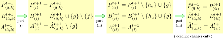
Figure 5.7: Partition of the stage for the terminal group into three parts in the proof that invariant (InvB) is preserved.

In the argument for the first two parts, we can assume that $f={f^{\ast}}\neq\varrho$ or $g={g^{\ast}}\neq h_{{\tilde{a}}}$ (or both), since if both $f=\varrho$ and $g=h_{{\tilde{a}}}$ then ${{{B}}^{t+1}_{(ii)}}={\dot{{B}}^{t+1}_{{\langle{{\tilde{a}}},k\rangle}}}={{{B}}^{t+1}_{{\mathrm{ins}}}}$, in which case invariant (InvB) holds after part (ii), as (InvB)(i) is trivial and (InvB)(ii) follows from the way ${{\mathcal{P}}}$ and ${{\mathcal{A}}}$ are modified in parts (i) and (ii). (Recall that $g\in{\left\{{g^{\ast}},h_{{{\tilde{a}}}}\right\}}$ and that $g=h_{{{\tilde{a}}}}$ iff ${{\tilde{a}}}=i_{l}$.)

Claim 5.12.

Assume that $f={f^{\ast}}\neq\varrho$ or $g={g^{\ast}}\neq h_{{\tilde{a}}}$. Then set ${{{B}}^{t+1}_{(i)}}={\dot{{B}}^{t+1}_{{\langle{{\tilde{a}}},k\rangle}}}\cup{\left\{g\right\}}\setminus{\left\{f\right\}}$ is a feasible set of packets pending at time $t+1$.

Proof.

Recall that ${\dot{{P}}^{t+1}_{{\langle{{\tilde{a}}},k\rangle}}}={{{P}}^{t+1}_{{\mathrm{ins}}}}$ and that the same relations hold for sets ${{\mathcal{B}}}$ and ${{\mathcal{A}}}$. Also, we are currently in Case L.$(\beta,\gamma]$.I.2, in which either $\varrho\in{{{B}}^{t+1}_{{\mathrm{ins}}}}$ or ${{{A}}^{t+1}_{{\mathrm{ins}}}}(\beta,\gamma]\neq\emptyset$.

The claim clearly holds if $d^{t}_{f}\leq d^{t}_{g}$. Otherwise, by the definition of tight slots, it suffices to prove $d^{t}_{f}\leq\textsf{nextts}({{{B}}^{t+1}_{{\mathrm{ins}}}},d^{t}_{g})$, from which the feasibility of ${{{B}}^{t+1}_{(i)}}$ follows. In particular, we show that ${\textsf{pslack}}({{{B}}^{t+1}_{{\mathrm{ins}}}},\tau)\geq 1$ for any $\tau\in[d^{t}_{g},d^{t}_{f})$.

We now consider two cases. First, assume that $\varrho\notin{{{B}}^{t+1}_{{\mathrm{ins}}}}$. This implies $f={f^{\ast}}$ and ${{{A}}^{t+1}_{{\mathrm{ins}}}}(\beta,\gamma]\neq\emptyset$, which means that $d^{t}_{g}\in(\beta,\gamma]$, no matter whether $g=h_{{\tilde{a}}}$ or $g={g^{\ast}}$. Then, for $\tau\in[d^{t}_{g},d^{t}_{f})$, Lemma 5.4(a) with $\zeta=\beta$ gives us

$${\textsf{pslack}}({{{B}}^{t+1}_{{\mathrm{ins}}}},\tau)\;\geq\;{\textsf{pslack}}({{{P}}^{t+1}_{{\mathrm{ins}}}},\tau)+|{{{A}}^{t+1}_{{\mathrm{ins}}}}(\beta,\tau]|\;\geq\;1,$$

since ${{{A}}^{t+1}_{{\mathrm{ins}}}}(\beta,\tau]$ contains $g$ and ${\textsf{pslack}}({{{P}}^{t+1}_{{\mathrm{ins}}}},\tau)\geq 0$.

Otherwise, $\varrho\in{{{B}}^{t+1}_{{\mathrm{ins}}}}\setminus{{{P}}^{t+1}_{{\mathrm{ins}}}}$, so $f=\varrho$. In this case, $g={g^{\ast}}$ holds (as we assume in this part that $f={f^{\ast}}\neq\varrho$ or $g={g^{\ast}}\neq h_{{\tilde{a}}}$). For $\tau\in[d^{t}_{g},d^{t}_{f})$, we use Lemma 5.4(b) with $\zeta=\gamma$ to obtain

$${\textsf{pslack}}({{{B}}^{t+1}_{{\mathrm{ins}}}},\tau)\;\geq\;{\textsf{pslack}}({{{P}}^{t+1}_{{\mathrm{ins}}}},\tau)+|{{{B}}^{t+1}_{{\mathrm{ins}}}}(\tau,\gamma]\setminus{{{P}}^{t+1}_{{\mathrm{ins}}}}|\;\geq\;1,$$

where we use $f=\varrho\in{{{B}}^{t+1}_{{\mathrm{ins}}}}(\tau,\gamma]\setminus{{{P}}^{t+1}_{{\mathrm{ins}}}}$ in the second inequality. ∎

From the definitions of ${{{P}}^{t+1}_{(i)}}$, ${{{A}}^{t+1}_{(i)}}$, and ${{{B}}^{t+1}_{(i)}}$, and using Claim 5.12, invariants (InvA) and (InvB) hold for these three intermediate sets.

Before considering part (ii) (that is, replacing $h_{{\tilde{a}}}$ by $\varrho$ in ${{\mathcal{P}}}$ and ${{\mathcal{B}}}$), we prove the following claim:

Claim 5.13.

Assume that $f={f^{\ast}}\neq\varrho$ or $g={g^{\ast}}\neq h_{{\tilde{a}}}$. If $d^{t}_{\varrho}<d^{t}_{h_{{\tilde{a}}}}$, then ${{\tilde{a}}}=k$ and ${\textsf{pslack}}({{{B}}^{t+1}_{(i)}},\tau)\geq 1$ for any $\tau\in[d^{t}_{\varrho},d^{t}_{h_{{\tilde{a}}}})$.

Proof.

Let $\chi=\textsf{prevts}^{t}(d^{t}_{\varrho})$. By the definitions of $\gamma$ and $\varrho$ and since the tight slots of ${{{P}}^{t+1}_{{\mathrm{ins}}}}$ are the same as those of ${{{P}}^{t}}$ starting with slot $\alpha$, $d^{t}_{\varrho}$ is in the segment $(\chi,\gamma]$ of ${{{P}}^{t+1}_{(i)}}={{{P}}^{t+1}_{{\mathrm{ins}}}}$; consequently, $d^{t}_{h_{{\tilde{a}}}}$ also belongs to this segment. So ${{\tilde{a}}}=k$, proving the first part of the claim. Moreover, it follows that ${\textsf{pslack}}({{{P}}^{t+1}_{(i)}},\tau)\geq 1$ for $\tau\in[d^{t}_{\varrho},d^{t}_{h_{k}})$.

We now make two observations that will be used later to prove Claim 5.13. First, observe that replacing $f$ by $g$ in ${{\mathcal{B}}}$ results in

$${\textsf{pslack}}({{{B}}^{t+1}_{(i)}},\tau)={\textsf{pslack}}({{{B}}^{t+1}_{{\mathrm{ins}}}},\tau)+1\geq 1\quad\textrm{for}\;\tau\in[d^{t}_{f},d^{t}_{g})\,,$$ (5.53)

where the inequality follows from the feasibility of ${{{B}}^{t+1}_{{\mathrm{ins}}}}$. (It is possible that $d^{t}_{g}\leq d^{t}_{f}$, in which case this interval is empty.)

Next, let ${\hat{f}}$ be the earliest-deadline packet in ${{{B}}^{t+1}_{(i)}}(\chi,T]\setminus{{{P}}^{t+1}_{(i)}}$ and let ${\hat{g}}$ be the latest-deadline packet in ${{{A}}^{t+1}_{(i)}}[t+1,\gamma]$; if ${\hat{f}}$ is undefined, we let $d^{t}_{\hat{f}}=T$, and similarly if ${\hat{g}}$ is undefined, we let $d^{t}_{\hat{g}}=t+1$. By Lemma 5.4 (which we can apply because invariants (InvA) and (InvB) are true for ${{{P}}^{t+1}_{(i)}}$, ${{{A}}^{t+1}_{(i)}}$, and ${{{B}}^{t+1}_{(i)}}$), it holds that

$${\textsf{pslack}}({{{B}}^{t+1}_{(i)}},\tau)\geq{\textsf{pslack}}({{{P}}^{t+1}_{(i)}},\tau)\geq 1\quad\textrm{for}\;\tau\in(\chi,\min(d^{t}_{\hat{f}},\gamma))\cup[\max(d^{t}_{\hat{g}},\chi+1),\gamma).$$ (5.54)

Specifically, we apply Lemma 5.4(a) with $\zeta=\chi$ to derive the first inequality for $\tau\in(\chi,d^{t}_{\hat{f}})$, and Lemma 5.4(b) with $\zeta=\gamma$ to derive the first inequality for $\tau\in[d^{t}_{\hat{g}},\gamma)$. The second inequality holds because $(\chi,\gamma]$ is a segment of ${{{P}}^{t+1}_{(i)}}$.

If $d^{t}_{\hat{f}}\geq\gamma$ or $d^{t}_{\hat{g}}\leq\chi$, then inequality (5.54) directly implies the lemma, because $[d^{t}_{\varrho},d^{t}_{h_{k}})\subseteq(\chi,\gamma)$. Therefore, for the rest of the proof, we will assume that $d^{t}_{\hat{f}}<\gamma$ and $d^{t}_{\hat{g}}>\chi$.

To complete the proof, it is sufficient to show that inequalities (5.53) and (5.54) cover the whole range of $\tau\in[d^{t}_{\varrho},d^{t}_{h_{k}})$, that is

$$[d^{t}_{\varrho},d^{t}_{h_{k}})\subseteq(\chi,d^{t}_{\hat{f}})\cup[d^{t}_{f},d^{t}_{g})\cup[d^{t}_{\hat{g}},\gamma).$$ (5.55)

Note that $d^{t}_{\hat{g}}\leq d^{t}_{g^{\ast}}$ and $d^{t}_{\hat{f}}\geq d^{t}_{f^{\ast}}$ by the definitions of these packets and of ${{{B}}^{t+1}_{(i)}}$ and ${{{A}}^{t+1}_{(i)}}$ (note that $g$ is not a candidate for ${\hat{f}}$ as $g\in{{{P}}^{t+1}_{(i)}}$). If $f=\varrho$, then it holds that $g={g^{\ast}}$ by the assumption, and the interval $[d^{t}_{\varrho},d^{t}_{h_{k}})$ is covered by $[d^{t}_{f},d^{t}_{g})=[d^{t}_{\varrho},d^{t}_{g^{\ast}})$ and $[d^{t}_{\hat{g}},\gamma)$, because $d^{t}_{\hat{g}}\leq d^{t}_{g^{\ast}}$ and $d^{t}_{h_{k}}\leq\gamma$. Similarly, if $g=h_{k}$, we have $f={f^{\ast}}$ and $[d^{t}_{\varrho},d^{t}_{h_{k}})$ is covered by $[d^{t}_{f},d^{t}_{g})=[d^{t}_{f^{\ast}},d^{t}_{h_{k}})$ and $(\chi,d^{t}_{\hat{f}})$, since $d^{t}_{\hat{f}}\geq d^{t}_{f^{\ast}}$. Finally, consider the case of $f={f^{\ast}}$ and $g={g^{\ast}}$. Then the interval $[d^{t}_{\varrho},d^{t}_{h_{k}})\subseteq(\chi,\gamma)$ is covered by $(\chi,d^{t}_{f^{\ast}})\cup[d^{t}_{f^{\ast}},d^{t}_{g^{\ast}})\cup[d^{t}_{g^{\ast}},\gamma)$, which implies (5.55), because $d^{t}_{\hat{f}}\geq d^{t}_{f^{\ast}}$ and $d^{t}_{\hat{g}}\leq d^{t}_{g^{\ast}}$. ∎

We now address the second part, where ${{{B}}^{t+1}_{(i)}}$ is changed into ${{{B}}^{t+1}_{(ii)}}={{{B}}^{t+1}_{(i)}}\setminus{\left\{h_{{\tilde{a}}}\right\}}\cup{\left\{\varrho\right\}}$, and we show that ${{{B}}^{t+1}_{(ii)}}$ satisfies invariant (InvB). We consider the feasibility of ${{{B}}^{t+1}_{(ii)}}$ first. Recall that in this part we assume $f={f^{\ast}}$ or $g={g^{\ast}}$. If $d^{t}_{\varrho}\geq d^{t}_{h_{{\tilde{a}}}}$, then the feasibility of ${{\mathcal{B}}}$ is clearly preserved after replacing $h_{{\tilde{a}}}$ by $\varrho$. Otherwise, $d^{t}_{\varrho}<d^{t}_{h_{{\tilde{a}}}}$, in which case, by Claim 5.13, we have ${{\tilde{a}}}=k$ and ${\textsf{pslack}}({{{B}}^{t+1}_{(ii)}},\tau)={\textsf{pslack}}({{{B}}^{t+1}_{(i)}},\tau)-1\geq 0$ for $\tau\in[d^{t}_{\varrho},d^{t}_{h_{{\tilde{a}}}})$; while ${\textsf{pslack}}({{{B}}^{t+1}_{(ii)}},\tau)={\textsf{pslack}}({{{B}}^{t+1}_{(i)}},\tau)\geq 0$ for $\tau\notin[d^{t}_{\varrho},d^{t}_{h_{{\tilde{a}}}})$, by Claim 5.12. Therefore, ${{{B}}^{t+1}_{(ii)}}$ is indeed feasible. In this part, we replace $h_{\tilde{a}}$ by $\varrho$ in both ${{\mathcal{P}}}$ and ${{\mathcal{B}}}$ and ${{\mathcal{A}}}$ is unchanged, so invariant (InvB)(ii) is preserved as well.

Finally, we consider the third part of this stage where the deadline decreases of $h_{{{\tilde{a}}}+1},\dots,h_{k}$ are implemented, converting ${{{B}}^{t+1}_{(ii)}}$ into ${\ddot{{B}}^{t+1}_{{\langle{{\tilde{a}}},k\rangle}}}$. (Unlike in the first two parts, we perform this part also in the case $f=\varrho$ and $g=h_{{\tilde{a}}}$.) We only need to show that ${\ddot{{B}}^{t+1}_{{\langle{{\tilde{a}}},k\rangle}}}$ remains feasible, since invariant (InvB)(ii) is not affected.

There is no deadline decrease in this part if ${{\tilde{a}}}=k$, so it remains to deal with the case when ${{\tilde{a}}}<k$. Recall that the algorithm will change the deadline $d^{t}_{h_{i}}$ to $d^{t+1}_{h_{i}}=\tau_{i-1}$, for each $i={{\tilde{a}}}+1,...,k$. These changes result in decreasing ${\textsf{pslack}}({{\mathcal{B}}})$ by one in each interval $[\tau_{{\tilde{a}}},d^{t}_{h_{{{\tilde{a}}}+1}}),\dots,[\tau_{k-1},d^{t}_{h_{k}})$. Other slots in ${{\mathcal{B}}}$ are not affected. These intervals are disjoint, because $d^{t}_{h_{i}}\leq\tau_{i}$ for $i=0,\dots,k$. Thus, it suffices to show the following claim.

Claim 5.14.

Assume that ${{\tilde{a}}}<k$. Then ${\textsf{pslack}}({{{B}}^{t+1}_{(ii)}},\tau)\geq 1$ for any $\tau\in[\tau_{{\tilde{a}}},\gamma)$.

Proof.

We first show that ${\textsf{pslack}}({{{P}}^{t+1}_{(ii)}},\tau)\geq 1$ for any $\tau\in[\tau_{{\tilde{a}}},\gamma)$. To this end, we consider two cases.

The first case is when $\tau\in[\tau_{{\tilde{a}}},d^{t}_{\varrho})$. For such $\tau$ we have ${\textsf{pslack}}({{{P}}^{t+1}_{(ii)}},\tau)\geq{\textsf{pslack}}({{{P}}^{t+1}_{(i)}},\tau)+1\geq 1$, because replacing $h_{{\tilde{a}}}$ by $\varrho$ causes ${\textsf{pslack}}({{\mathcal{P}}},\tau)$ to increase by 1 for $\tau\in[d^{t}_{h_{{\tilde{a}}}},d^{t}_{\varrho})\supseteq[\tau_{{\tilde{a}}},d^{t}_{\varrho})$, and because ${{{P}}^{t+1}_{(i)}}={{{P}}^{t+1}_{{\mathrm{ins}}}}$ is feasible.

The second case is when $\tau\in[d^{t}_{\varrho},\gamma)$. In this case we argue as follows. Since for ${{\tilde{a}}}<k$ replacing $h_{{\tilde{a}}}$ by $\varrho$ in ${{\mathcal{P}}}$ does not decrease any value ${\textsf{pslack}}({{\mathcal{P}}},\tau)$ (i.e., there are no new tight slots in ${{\mathcal{P}}}$) and each slot $\tau\in[d^{t}_{\varrho},\gamma)$ belongs to the segment of ${{{P}}^{t+1}_{(ii)}}$ ending at $\gamma$, we indeed have ${\textsf{pslack}}({{{P}}^{t+1}_{(ii)}},\tau)\geq 1$ for any $\tau\in[d^{t}_{\varrho},\gamma)$.

We thus have ${\textsf{pslack}}({{{P}}^{t+1}_{(ii)}},\tau)\geq 1$ for all $\tau\in[\tau_{{\tilde{a}}},\gamma)$, as claimed. To finish the proof, note that $d^{t}_{g^{\ast}}\leq\tau_{{\tilde{a}}}$ by the definitions of ${g^{\ast}}$ and the terminal group ${\langle{{\tilde{a}}},k\rangle}$, and that ${{{A}}^{t+1}_{(ii)}}(\tau_{{\tilde{a}}},\gamma]=\emptyset$. Thus for $\tau\in[\tau_{{\tilde{a}}},\gamma)$, we can apply Lemma 5.4(b) with $\zeta=\gamma$ to obtain ${\textsf{pslack}}({{{B}}^{t+1}_{(ii)}},\tau)\geq{\textsf{pslack}}({{{P}}^{t+1}_{(ii)}},\tau)\geq 1$, completing the proof. ∎

Putting it all together and using Claim 5.14, we obtain that ${\textsf{pslack}}({\ddot{{B}}^{t+1}_{{\langle{{\tilde{a}}},k\rangle}}},\tau)\geq{\textsf{pslack}}({{{B}}^{t+1}_{(ii)}},\tau)-1\geq 0$ for any $\tau\in[\tau_{{\tilde{a}}},\gamma)$, while ${\textsf{pslack}}({\ddot{{B}}^{t+1}_{{\langle{{\tilde{a}}},k\rangle}}},\tau)={\textsf{pslack}}({{{B}}^{t+1}_{(ii)}},\tau)\geq 0$ for $\tau\notin[\tau_{{\tilde{a}}},\gamma)$. This concludes the proof that invariant (InvB) holds after the stage for the terminal group.

Stage for a middle group.

We now analyze the stage in which the segments represented by a middle group ${\langle a,b\rangle}$ of indices are processed. The current intermediate plan, backup plan, and adversary stash are ${\dot{{P}}^{t+1}_{{\langle a,b\rangle}}}$, ${\dot{{B}}^{t+1}_{{\langle a,b\rangle}}}$, and ${\dot{{A}}^{t+1}_{{\langle a,b\rangle}}}$, respectively, and we assume that they satisfy invariants (InvA) and (InvB). At this point, it holds that:

1. $h_{a}\in{\dot{{A}}^{t+1}_{{\langle a,b\rangle}}}$ by the definition of the middle group,

2. $h_{b+1}\notin{\dot{{P}}^{t+1}_{{\langle a,b\rangle}}}$ as a result of the previous stage (recall that $b<k$ for a middle group), which implies that $h_{b+1}\notin{\dot{{A}}^{t+1}_{{\langle a,b\rangle}}}$ by invariant (InvA), and

3. $h_{b+1}\notin{\dot{{B}}^{t+1}_{{\langle a,b\rangle}}}$, because $h_{b+1}$ was removed from ${\mathcal{P}}$ in the previous stage (that is, we had $h_{b+1}\in{{{P}}^{t}}(\alpha,{T}]$, but now $h_{b+1}\notin{\dot{{P}}^{t+1}_{{\langle a,b\rangle}}}$), and because we do not add any packets to ${{\mathcal{B}}}(\alpha,{T}]\setminus{{\mathcal{P}}}$ while processing a leap step (see the “monotonicity of ${{\mathcal{B}}}\setminus{{\mathcal{P}}}$” invariant in Section 5.5.3).

The changes of plan ${{\mathcal{P}}}$ in this stage involve removing $h_{a}$ and adding back $h_{b+1}$; that is ${\dot{{P}}^{t+1}_{{\langle a,b\rangle}}}$ is changed to ${\ddot{{P}}^{t+1}_{{\langle a,b\rangle}}}={\dot{{P}}^{t+1}_{{\langle a,b\rangle}}}\setminus{\left\{h_{a}\right\}}\cup{\left\{h_{b+1}\right\}}$. We also decrease the deadlines of packets $h_{a+1},\dots,h_{b+1}$ and increase the weights of a subset of packets $h_{a+1},\dots,h_{b+1}$, according to the algorithm. Since $h_{a}$ is removed from ${{\mathcal{P}}}$, we also need to remove it from ${{\mathcal{A}}}$ to preserve invariant (InvA). Similarly, as $h_{b+1}$ is added back to ${{\mathcal{P}}}$ (and is not in ${{\mathcal{A}}}$), it needs to be added to ${{\mathcal{B}}}$ or to ${{\mathcal{A}}}$ so that invariant (InvB)(ii) continues to hold. The changes of ${{\mathcal{A}}}$ and ${{\mathcal{B}}}$ depend on two cases, which are described below.

Case L.$(\beta,\gamma]$.M.1: There is an index $i\in[a+1,b+1]$ such that $w^{t}_{h_{i}}<\mu_{i-1}$, i.e., the algorithm (in line 11) increases the weight of $h_{i}$. We will remove $h_{a}$ from ${{\mathcal{A}}}$ and add $h_{b+1}$ to ${{\mathcal{B}}}$. To restore the feasibility of ${{\mathcal{B}}}$, we apply Lemma 5.5 for packet $g=h_{a}$ to identify a packet $f_{a}\in{\dot{{B}}^{t+1}_{{\langle a,b\rangle}}}\setminus{\dot{{P}}^{t+1}_{{\langle a,b\rangle}}}$ for which set ${\dot{{B}}^{t+1}_{{\langle a,b\rangle}}}\setminus{\left\{f_{a}\right\}}\cup{\left\{h_{a}\right\}}$ is feasible and $d^{t}_{f_{a}}>\textsf{prevts}({\dot{{P}}^{t+1}_{{\langle a,b\rangle}}},d^{t}_{h_{a}})$. We then let

$${\ddot{{A}}^{t+1}_{{\langle a,b\rangle}}}\;=\;{\dot{{A}}^{t+1}_{{\langle a,b\rangle}}}\setminus{\left\{h_{a}\right\}}\quad\textrm{and}\quad{\ddot{{B}}^{t+1}_{{\langle a,b\rangle}}}\;=\;{\dot{{B}}^{t+1}_{{\langle a,b\rangle}}}\setminus{\left\{f_{a}\right\}}\cup{\left\{h_{b+1}\right\}}\,.$$

With these changes, (InvA) is preserved, since also none of packets $h_{a+1},\dots,h_{b+1}$, whose deadlines are decreased, is in ${\ddot{{A}}^{t+1}_{{\langle a,b\rangle}}}$. We will show below that ${\ddot{{B}}^{t+1}_{{\langle a,b\rangle}}}$ is feasible, even with the deadlines of $h_{a+1},\dots,h_{b+1}$ decreased by the algorithm.

Deriving (5.43) in Case L.$(\beta,\gamma]$.M.1. We need to take into account the addition of $h_{b+1}$ in ${{\mathcal{B}}}$ and possible change of weights of some packets $h_{a+1},\dots,h_{b+1}$. Taking these changes into account, the terms on the left-hand side of (5.43) can be expressed or estimated as follows:

$$\Delta_{{\langle a,b\rangle}}\Psi\; =\;{\textstyle{\frac{1}{\phi}}}{\,}\left(\Delta^{t}w({h_{a+1}},\dots,{h_{b+1}})+w^{t}_{h_{b+1}}-w^{t}_{f_{a}}\right)$$ (5.56)

$$\Delta^{t}w({h_{a+1}},\dots,{h_{b+1}})\; \leq\;\mu_{a}-w^{t}_{h_{b+1}}$$ (5.57)

$$\textsf{advcredit}^{t}_{{\langle a,b\rangle}}\; =\;w^{t}_{h_{a}}-{\textsf{minwt}}({\dot{{P}}^{t+1}_{{\langle a,b\rangle}}},d^{t}_{h_{a}})\;\leq\;w^{t}_{h_{a}}-\mu_{a}$$ (5.58)

To justify (5.56), note that while $h_{b+1}\notin{\dot{{B}}^{t+1}_{{\langle a,b\rangle}}}$ is added to ${{\mathcal{B}}}$ with its new weight $w^{t+1}_{h_{b+1}}$, its weight increase of $w^{t+1}_{h_{b+1}}-w^{t}_{h_{b+1}}$ is already accounted for in $\Delta^{t}w({h_{a+1}},\dots,{h_{b+1}})$.

Inequality (5.57) can be derived from the case condition, which says that there is $i\in[a+1,b+1]$ such that $w^{t}_{h_{i}}<\mu_{i-1}$, so we just need to apply Lemma 5.11 with $a^{\prime}=a+1$ and $b^{\prime}=b+1$ to get (5.57).

Inequality (5.58) follows from the definition of $\mu_{a}$ as $\mu_{a}={\textsf{minwt}}({P}^{t},d^{t}_{h_{a}})$ and from the observation that ${\textsf{minwt}}({\dot{{P}}^{t+1}_{{\langle a,b\rangle}}},d^{t}_{h_{a}})\geq{\textsf{minwt}}({P}^{t},d^{t}_{h_{a}})$, which in turn follows from $\textsf{nextts}({\dot{{P}}^{t+1}_{{\langle a,b\rangle}}},d^{t}_{h_{a}})=\textsf{nextts}({P}^{t},d^{t}_{h_{a}})$ and ${\dot{{P}}^{t+1}_{{\langle a,b\rangle}}}[t+1,\eta]={P}^{t}[t,\eta]\setminus{\left\{{\ell}\right\}}$, where $\eta=\textsf{nextts}({\dot{{P}}^{t+1}_{{\langle a,b\rangle}}},d^{t}_{h_{a}})$. (The equality $\textsf{nextts}({\dot{{P}}^{t+1}_{{\langle a,b\rangle}}},d^{t}_{h_{a}})=\textsf{nextts}({P}^{t},d^{t}_{h_{a}})$ holds because of the “locality of changes” invariant from Section 5.5.3).

Next, we claim that

$$w^{t}_{f_{a}}\;\leq\;w^{t}_{h_{b+1}}.$$ (5.59)

Indeed, $f_{a}$ is not in ${P}^{t}$ since, by its definition, $f_{a}\notin{\dot{{P}}^{t+1}_{{\langle a,b\rangle}}}$ and $d^{t}_{f_{a}}>\textsf{prevts}({\dot{{P}}^{t+1}_{{\langle a,b\rangle}}}d^{t}_{h_{a}})\geq\beta$, so $f_{a}$ could not have been removed from ${{\mathcal{P}}}$ in this step. (Note that $h_{b+1}$ is temporarily removed from ${{\mathcal{P}}}$, but it cannot be equal $f_{a}$ because $h_{b+1}\notin{\dot{{B}}^{t+1}_{{\langle a,b\rangle}}}$). Thus $w^{t}_{f_{a}}\leq w^{t}_{\varrho}$, because $\varrho$ is the heaviest pending packet not in ${{{P}}^{t}}$ with deadline after $\beta$ and $f_{a}\notin{{{P}}^{t}}$ is pending in step $t$. By Lemma B.1(b) we have $w^{t}_{\varrho}\leq w^{t}_{h_{b+1}}$, which implies that $w^{t}_{f_{a}}\leq w^{t}_{h_{b+1}}$. (As an additional clarification, the argument in this paragraph relies tacitly on two properties of earlier changes in processing the transmission event: One, no packets with deadlines after $\alpha$ are added to ${{\mathcal{B}}}\setminus{{\mathcal{P}}}$, and two, the tight slots of ${\dot{{P}}^{t+1}_{{\langle a,b\rangle}}}$ in the interval $(\beta,\tau_{b}]$ are the same as tight slots in ${{{P}}^{t}}$; cf. Section 5.5.3.)

Then we prove (5.43) as follows:

$$\Delta_{{\langle a,b\rangle}}\Psi -\phi{\,}\Delta^{t}w({h_{a+1}},\dots,{h_{b+1}})-\textsf{advcredit}^{t}_{{\langle a,b\rangle}}$$

$$\geq\;{\textstyle{\frac{1}{\phi}}}{\,}\left(\Delta^{t}w({h_{a+1}},\dots,{h_{b+1}})+w^{t}_{h_{b+1}}-w^{t}_{f_{a}}\right)$$

$$\qquad\qquad-\phi{\,}\Delta^{t}w({h_{a+1}},\dots,{h_{b+1}})-(w^{t}_{h_{a}}-\mu_{a})$$

$$=\;{\textstyle{\frac{1}{\phi}}}{\,}\left(w^{t}_{h_{b+1}}-w^{t}_{f_{a}}\right)-\Delta^{t}w({h_{a+1}},\dots,{h_{b+1}})-w^{t}_{h_{a}}+\mu_{a}$$

$$\geq\;-(\mu_{a}-w^{t}_{h_{b+1}})-w^{t}_{h_{a}}+\mu_{a}$$ (5.60)

$$=\;-w^{t}_{h_{a}}+w^{t}_{h_{b+1}}\,,$$

where inequality (5.60) follows from (5.59) and (5.57).

Invariant (InvB) in Case L.$(\beta,\gamma]$.M.1. We claim that after the stage for the middle group ${\langle a,b\rangle}$, invariant (InvB) holds, which we show by partitioning this stage into three parts:

(i) We first let ${{{B}}^{t+1}_{(i)}}={\dot{{B}}^{t+1}_{{\langle a,b\rangle}}}\setminus{\left\{f_{a}\right\}}\cup{\left\{h_{a}\right\}}$.

(ii) Second, we modify ${{{B}}^{t+1}_{(i)}}$ to obtain set ${{{B}}^{t+1}_{(ii)}}={{{B}}^{t+1}_{(i)}}\setminus{\left\{h_{a}\right\}}\cup{\left\{h_{b+1}\right\}}$.

(iii) Finally, we implement the decrease of the deadlines of packets $h_{a+1},\dots,h_{b+1}$, changing ${{{B}}^{t+1}_{(ii)}}$ to ${\ddot{{B}}^{t+1}_{{\langle a,b\rangle}}}$.

In each part, we also appropriately modify the sets ${{\mathcal{P}}}$ and ${{\mathcal{A}}}$, as illustrated in Figure 5.8.

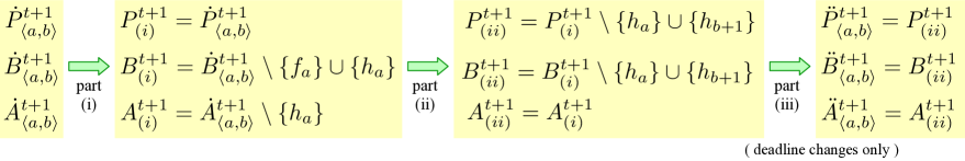
Figure 5.8: Partition of the stage for the middle group in Case L.$(\beta,\gamma]$.M.1 into three parts.

That ${{{B}}^{t+1}_{(i)}}$ is feasible follows from the choice of $f_{a}$ and Lemma 5.5. Since $d^{t}_{h_{a}}<d^{t}_{h_{b+1}}$, ${{{B}}^{t+1}_{(ii)}}$ is also a feasible set of packets, and moreover, ${\textsf{pslack}}({{{B}}^{t+1}_{(ii)}},\tau)={\textsf{pslack}}({{{B}}^{t+1}_{(i)}},\tau)+1\geq 1$ for any $\tau\in[d^{t}_{h_{a}},d^{t}_{h_{b+1}})$, by the feasibility of ${{{B}}^{t+1}_{(i)}}$. Finally, we argue that ${\ddot{{B}}^{t+1}_{{\langle a,b\rangle}}}$ remains feasible. The deadline decreases for packets $h_{a+1},\dots,h_{b+1}$ decrease ${\textsf{pslack}}({{\mathcal{B}}})$ by one for slots in each of the disjoint intervals $[\tau_{a},d^{t}_{h_{a+1}}),\dots,[\tau_{b},d^{t}_{h_{b+1}})$. As $d^{t}_{h_{a}}\leq\tau_{a}$, all these intervals are contained in $[d^{t}_{h_{a}},d^{t}_{h_{b+1}})$; hence, by the earlier observation, it holds that ${\textsf{pslack}}({\ddot{{B}}^{t+1}_{{\langle a,b\rangle}}},\tau)\geq{\textsf{pslack}}({{{B}}^{t+1}_{(ii)}},\tau)-1\geq 0$ for any $\tau\in[d^{t}_{h_{a}},d^{t}_{h_{b+1}})$. For $\tau\notin[d^{t}_{h_{a}},d^{t}_{h_{b+1}})$, the values of ${\textsf{pslack}}({{\mathcal{B}}})$ do not change. It follows that ${\ddot{{B}}^{t+1}_{{\langle a,b\rangle}}}$ is feasible; that is, invariant (InvB)(i) holds after the stage. That invariant (InvB)(ii) holds as well follows directly from the definitions of ${\ddot{{P}}^{t+1}_{{\langle a,b\rangle}}}$, ${\ddot{{B}}^{t+1}_{{\langle a,b\rangle}}}$, and ${\ddot{{A}}^{t+1}_{{\langle a,b\rangle}}}$.

Case L.$(\beta,\gamma]$.M.2: For all indices $i\in[a+1,b+1]$ we have $w^{t}_{h_{i}}\geq\mu_{i-1}$. Thus in this case the algorithm does not increase the weights of packets $h_{a+1},...,h_{b+1}$, i.e., $\Delta^{t}w({h_{a+1}},\dots,{h_{b+1}})=0$.

Before describing the changes in ${{\mathcal{A}}}$, we argue that $h_{a+1}\notin{\dot{{A}}^{t+1}_{{\langle a,b\rangle}}}$. This is trivial if $b>a$, because then packets $h_{a+1},\dots,h_{b}$ are not in ${{\mathcal{A}}}$ before processing the groups. Otherwise, we have $a=b$. Since in the stages, we process the groups backwards with respect to time slots, the stage for the group ${\langle b+1,b^{\prime}\rangle}$ containing index $b+1$ is already completed, and it guarantees that $h_{b+1}$ is not in ${\ddot{{P}}^{t+1}_{{\langle b+1,b^{\prime}\rangle}}}={\dot{{P}}^{t+1}_{{\langle a,b\rangle}}}$ and thus not in ${\ddot{{A}}^{t+1}_{{\langle b+1,b^{\prime}\rangle}}}={\dot{{A}}^{t+1}_{{\langle a,b\rangle}}}$ by invariant (InvA), as claimed. (See also the overview of the partition into stages, earlier in the description of Case L.$(\beta,\gamma]$.I.2.)

We now change ${{\mathcal{A}}}$ as follows: we remove $h_{a}$ from ${{\mathcal{A}}}$, and we put $h_{a+1}$ in the former slot of $h_{a}$ in ${\dot{{A}}^{t+1}_{{\langle a,b\rangle}}}$, that is ${\ddot{{A}}^{t+1}_{{\langle a,b\rangle}}}={\dot{{A}}^{t+1}_{{\langle a,b\rangle}}}\setminus{\left\{h_{a}\right\}}\cup{\left\{h_{a+1}\right\}}$. This is valid because, as we showed above, $h_{a+1}\notin{\dot{{A}}^{t+1}_{{\langle a,b\rangle}}}$, and the new deadline of $h_{a+1}$ is $\tau_{a}$. Then $\textsf{advcredit}^{t}_{{\langle a,b\rangle}}=w^{t}_{h_{a}}-w^{t}_{h_{a+1}}$, as the weight of $h_{a+1}$ does not change. Since packets $h_{a+2},\dots,h_{b+1}$ are not in ${\ddot{{A}}^{t+1}_{{\langle a,b\rangle}}}$, the decreases of their deadlines do not affect ${{\mathcal{A}}}$. After these changes, invariant (InvA) will be preserved.

Regarding ${{\mathcal{B}}}$, recall that $h_{b+1}\notin{\dot{{B}}^{t+1}_{{\langle a,b\rangle}}}$, $h_{a}\in{\dot{{A}}^{t+1}_{{\langle a,b\rangle}}}$, and $h_{a}\notin{\ddot{{P}}^{t+1}_{{\langle a,b\rangle}}}$. Also, if $b>a$ then $h_{a+1}\in{\dot{{B}}^{t+1}_{{\langle a,b\rangle}}}$. Then, since $h_{a+1}$ is newly added to ${{\mathcal{A}}}$, we let ${\ddot{{B}}^{t+1}_{{\langle a,b\rangle}}}={\dot{{B}}^{t+1}_{{\langle a,b\rangle}}}\cup{\left\{h_{b+1}\right\}}\setminus{\left\{h_{a+1}\right\}}$; it is possible here that $h_{a+1}=h_{b+1}$, in which case ${{\mathcal{B}}}$ does not change.

Deriving (5.43) in Case L.$(\beta,\gamma]$.M.2. In this case, the terms on the left-hand side of (5.43) are

$$\Delta_{{\langle a,b\rangle}}\Psi\; =\;{\textstyle{\frac{1}{\phi}}}{\,}\left(-w^{t}_{h_{a+1}}+w^{t}_{h_{b+1}}\right)$$

$$\Delta^{t}w({h_{a+1}},\dots,{h_{b+1}})\; =\;0$$

$$\textsf{advcredit}^{t}_{{\langle a,b\rangle}}\; =\;w^{t}_{h_{a}}-w^{t}_{h_{a+1}}$$

with all formulas following directly from the definition and the fact that the weights remain unchanged. Plugging these in, we obtain:

$$\Delta_{{\langle a,b\rangle}}\Psi -\phi{\,}\Delta^{t}w({h_{a+1}},\dots,{h_{b+1}})-\textsf{advcredit}^{t}_{{\langle a,b\rangle}}$$

$$=\;{\textstyle{\frac{1}{\phi}}}{\,}\left(-w^{t}_{h_{a+1}}+w^{t}_{h_{b+1}}\right)-\phi\cdot 0-(w^{t}_{h_{a}}-w^{t}_{h_{a+1}})$$

$$=\;-w^{t}_{h_{a}}+{\textstyle{\frac{1}{\phi^{2}}}}{\,}w^{t}_{h_{a+1}}+{\textstyle{\frac{1}{\phi}}}{\,}w^{t}_{h_{b+1}}$$

$$\geq\;-w^{t}_{h_{a}}+{\textstyle{\frac{1}{\phi^{2}}}}{\,}w^{t}_{h_{b+1}}+{\textstyle{\frac{1}{\phi}}}{\,}w^{t}_{h_{b+1}}$$ (5.61)

$$=\;-w^{t}_{h_{a}}+w^{t}_{h_{b+1}}\,,$$

where inequality (5.61) follows from $w^{t}_{h_{a+1}}\geq w^{t}_{h_{b+1}}$, by Lemma B.1(b) and $a\leq b$.

Invariant (InvB) in Case L.$(\beta,\gamma]$.M.2

We show that ${\ddot{{B}}^{t+1}_{{\langle a,b\rangle}}}$ is feasible by considering first an intermediate backup plan ${{{B}}^{t+1}_{(i)}}={\dot{{B}}^{t+1}_{{\langle a,b\rangle}}}\cup{\left\{h_{b+1}\right\}}\setminus{\left\{h_{a+1}\right\}}$, computed with packets $h_{a+1},\dots,h_{b+1}$ having their deadlines unchanged. Since ${{{B}}^{t+1}_{(i)}}$ is obtained by replacing $h_{a+1}$ by $h_{b+1}$ in ${{\mathcal{B}}}$, and $d^{t}_{h_{a+1}}\leq d^{t}_{h_{b+1}}$, ${{{B}}^{t+1}_{(i)}}$ is feasible; moreover, it satisfies ${\textsf{pslack}}({{{B}}^{t+1}_{(i)}},\tau)={\textsf{pslack}}({\dot{{B}}^{t+1}_{{\langle a,b\rangle}}},\tau)+1\geq 1$ for any $\tau\in[d^{t}_{h_{a+1}},d^{t}_{h_{b+1}})$. Next, to prove the feasibility of ${\ddot{{B}}^{t+1}_{{\langle a,b\rangle}}}$, we decrease the deadlines of packets $h_{a+1},\dots,h_{b+1}$. This decreases ${\textsf{pslack}}({{\mathcal{B}}})$ by one for slots in disjoint intervals $[\tau_{a+1},d^{t}_{h_{a+2}}),\dots,[\tau_{b},d^{t}_{h_{b+1}})$. (We do not consider $h_{a+1}$ here because this packet was already removed from ${{\mathcal{B}}}$.) These intervals are contained in $[d^{t}_{h_{a+1}},d^{t}_{h_{b+1}})$, and we thus have ${\textsf{pslack}}({\ddot{{B}}^{t+1}_{{\langle a,b\rangle}}},\tau)\geq{\textsf{pslack}}({{{B}}^{t+1}_{(i)}},\tau)-1\geq 0$ for $\tau\in[d^{t}_{h_{a+1}},d^{t}_{h_{b+1}})$. For $\tau\notin[d^{t}_{h_{a+1}},d^{t}_{h_{b+1}})$, the values of ${\textsf{pslack}}({{\mathcal{B}}})$ do not change. Therefore ${\ddot{{B}}^{t+1}_{{\langle a,b\rangle}}}$ is feasible, showing (InvB)(i). Part (ii) of invariant (InvB) is implied by the changes of sets ${{\mathcal{P}}},{{\mathcal{A}}}$, and ${{\mathcal{B}}}$.

This completes the proof that invariants (InvA) and (InvB) are preserved after the stage for the middle group ${\langle a,b\rangle}$, and that inequality (5.43) holds for this stage.

Stage for the initial group.

The initial group ${\langle 0,{{\tilde{b}}}\rangle}$ is defined when either $l>0$ and $i_{1}>0$ or if $l=0$ and ${{\tilde{a}}}>0$. In either case, we have $h_{0},...,h_{{\tilde{b}}}\not\in{\dot{{A}}^{t+1}_{{\langle 0,{{\tilde{b}}}\rangle}}}$.

In the stage in which this group is processed, we change plan ${{\mathcal{P}}}$ by removing $h_{0}=p$ and adding $h_{{{\tilde{b}}}+1}$, so ${\widetilde{{P}}^{t+1}}={\dot{{P}}^{t+1}_{{\langle 0,{{\tilde{b}}}\rangle}}}\setminus{\left\{p\right\}}\cup{\left\{h_{{{\tilde{b}}}+1}\right\}}$. (Recall that ${\widetilde{{P}}^{t+1}}={\ddot{{P}}^{t+1}_{{\langle 0,{{\tilde{b}}}\rangle}}}$ and the corresponding relation holds for ${{\mathcal{A}}}$ and ${{\mathcal{B}}}$, since we process the stage for the initial group after all other groups.) We also decrease the deadlines of packets $h_{1},\dots,h_{{{\tilde{b}}}+1}$, and for some we increase their weights, according to the algorithm. We do not change ${{\mathcal{A}}}$; thus ${\widetilde{{A}}^{t+1}}={\dot{{A}}^{t+1}_{{\langle 0,{{\tilde{b}}}\rangle}}}$ and $\textsf{advcredit}^{t}_{{\langle 0,{{\tilde{b}}}\rangle}}=0$. Since packets $h_{1},\dots,h_{{{\tilde{b}}}+1}$ are not in ${\dot{{A}}^{t+1}_{{\langle 0,{{\tilde{b}}}\rangle}}}$, it follows that invariant (InvA) is preserved. To update ${{\mathcal{B}}}$, we let ${\widetilde{{B}}^{t+1}}={\dot{{B}}^{t+1}_{{\langle 0,{{\tilde{b}}}\rangle}}}\setminus{\left\{p\right\}}\cup{\left\{h_{{{\tilde{b}}}+1}\right\}}$ (recall that $h_{{{\tilde{b}}}+1}\notin{\dot{{B}}^{t+1}_{{\langle 0,{{\tilde{b}}}\rangle}}}$).

Deriving (5.43) for the initial group. The terms on the left-hand side of (5.43) can be expressed or estimated as follows:

$$\Delta_{{\langle 0,{{\tilde{b}}}\rangle}}\Psi\; =\;{\textstyle{\frac{1}{\phi}}}{\,}\left(\Delta^{t}w({h_{1}},\dots,{h_{{{\tilde{b}}}+1}})-w^{t}_{p}+w^{t}_{h_{{{\tilde{b}}}+1}}\right)$$ (5.62)

$$\Delta^{t}w({h_{1}},\dots,{h_{{{\tilde{b}}}+1}})\; \leq\;{\textstyle{\frac{1}{\phi^{2}}}}{\,}(w^{t}_{p}-w^{t}_{h_{{{\tilde{b}}}+1}})$$ (5.63)

$$\textsf{advcredit}^{t}_{{\langle 0,{{\tilde{b}}}\rangle}}\; =\;0$$ (5.64)

Equations (5.62) and (5.64) follow directly from the definitions and the case assumption.

To justify (5.63), we consider two cases. If the algorithm does not increase the weight of any of the packets $h_{1},\dots,h_{{{\tilde{b}}}+1}$, then $\Delta^{t}w({h_{1}},\dots,{h_{{{\tilde{b}}}+1}})=0\leq{\textstyle{\frac{1}{\phi^{2}}}}{\,}(w^{t}_{p}-{\,}w^{t}_{h_{{{\tilde{b}}}+1}})$, by Lemma B.1(b). Otherwise, there is $i\in[1,{{\tilde{b}}}+1]$ such that $w^{t}_{h_{i}}<\mu_{i-1}$, and applying Lemma 5.11 with $a^{\prime}=1$ and $b^{\prime}={{\tilde{b}}}+1$, we obtain

$$\Delta^{t}w({h_{1}},\dots,{h_{{{\tilde{b}}}+1}})\; \leq\;\mu_{0}-w^{t}_{h_{{{\tilde{b}}}+1}}$$

$$\leq\;{\textstyle{\frac{1}{\phi^{2}}}}{\,}w^{t}_{p}+{\textstyle{\frac{1}{\phi}}}{\,}w^{t}_{\varrho}-w^{t}_{h_{{{\tilde{b}}}+1}}$$ (5.65)

$$\leq\;{\textstyle{\frac{1}{\phi^{2}}}}{\,}(w^{t}_{p}-w^{t}_{h_{{{\tilde{b}}}+1}})\,,$$ (5.66)

where inequality (5.65) uses the bound $\mu_{0}\leq{\textstyle{\frac{1}{\phi^{2}}}}{\,}w^{t}_{p}+{\textstyle{\frac{1}{\phi}}}{\,}w^{t}_{\varrho}$, that follows from (5.26), and inequality (5.66) uses $w^{t}_{\varrho}\leq w^{t}_{h_{{{\tilde{b}}}+1}}$, that follows from Lemma B.1(b). Thus (5.63) holds.

The calculation showing (5.43) is now quite simple:

$$\Delta_{{\langle 0,{{\tilde{b}}}\rangle}}\Psi -\phi{\,}\Delta^{t}w({h_{1}},\dots,{h_{{{\tilde{b}}}+1}})-\textsf{advcredit}^{t}_{{\langle 0,{{\tilde{b}}}\rangle}}$$

$$=\;{\textstyle{\frac{1}{\phi}}}{\,}\left(\Delta^{t}w({h_{1}},\dots,{h_{{{\tilde{b}}}+1}})-w^{t}_{p}+w^{t}_{h_{{{\tilde{b}}}+1}}\right)-\phi{\,}\Delta^{t}w({h_{1}},\dots,{h_{{{\tilde{b}}}+1}})-0$$

$$=\;{\textstyle{\frac{1}{\phi}}}{\,}(-w^{t}_{p}+w^{t}_{h_{{{\tilde{b}}}+1}})-\Delta^{t}w({h_{1}},\dots,{h_{{{\tilde{b}}}+1}})$$

$$\geq\;{\textstyle{\frac{1}{\phi}}}{\,}(-w^{t}_{p}+w^{t}_{h_{{{\tilde{b}}}+1}})-{\textstyle{\frac{1}{\phi^{2}}}}{\,}(w^{t}_{p}-w^{t}_{h_{{{\tilde{b}}}+1}})$$ (5.67)

$$=\;-w^{t}_{p}+w^{t}_{h_{{{\tilde{b}}}+1}}\,,$$

where inequality(5.67) holds by (5.63).

Invariant (InvB) after the stage for the initial group. That invariant (InvB)(ii) is preserved follows directly from the formulas for ${\widetilde{{P}}^{t+1}}$, ${\widetilde{{B}}^{t+1}}$, and ${\widetilde{{A}}^{t+1}}$.

To show invariant (InvB)(i), that is the feasibility of ${\widetilde{{B}}^{t+1}}$, we consider an intermediate backup plan ${{{B}}^{t+1}_{(i)}}={\dot{{B}}^{t+1}_{{\langle 0,{{\tilde{b}}}\rangle}}}\setminus{\left\{p\right\}}\cup{\left\{h_{{{\tilde{b}}}+1}\right\}}$, where the deadlines of packets $h_{1},\dots,h_{{{\tilde{b}}}+1}$ remain unchanged. Replacing $p$ by $h_{{{\tilde{b}}}+1}$ in ${{\mathcal{B}}}$ preserves feasibility as $d^{t}_{p}<d^{t}_{h_{{{\tilde{b}}}+1}}$. So ${{{B}}^{t+1}_{(i)}}$ is feasible; moreover, it satisfies ${\textsf{pslack}}({{{B}}^{t+1}_{(i)}},\tau)={\textsf{pslack}}({\dot{{B}}^{t+1}_{{\langle 0,{{\tilde{b}}}\rangle}}},\tau)+1\geq 1$ for any $\tau\in[d^{t}_{p},d^{t}_{h_{{{\tilde{b}}}+1}})$.

We now decrease the deadlines of packets $h_{1},\dots,h_{{{\tilde{b}}}+1}$, as in the algorithm. This decreases ${\textsf{pslack}}({{\mathcal{B}}},\tau)$ by one for slots $\tau$ in disjoint intervals $[\tau_{0},d^{t}_{h_{1}}),\dots,[\tau_{{\tilde{b}}},d^{t}_{h_{{{\tilde{b}}}+1}})$. These intervals are contained in $[d^{t}_{p},d^{t}_{h_{{{\tilde{b}}}+1}})$, and we thus have ${\textsf{pslack}}({\widetilde{{B}}^{t+1}},\tau)\geq{\textsf{pslack}}({{{B}}^{t+1}_{(i)}},\tau)-1\geq 0$ for $\tau\in[d^{t}_{p},d^{t}_{h_{{{\tilde{b}}}+1}})$. The values of ${\textsf{pslack}}({{\mathcal{B}}})$ are not affected for slots $\tau\notin[d^{t}_{p},d^{t}_{h_{{{\tilde{b}}}+1}})$. Therefore ${\widetilde{{B}}^{t+1}}$ is feasible; that is, invariant (InvB)(i) holds after the stage for the initial group and after the algorithm’s step as well.

Summary of Case L.$\boldsymbol{(\beta,\gamma]}$.I.2.

In this case, we processed changes in the interval $(\beta,\gamma]$ when $\varrho\in{{{B}}^{t+1}_{{\mathrm{ins}}}}$ or ${{{A}}^{t+1}_{{\mathrm{ins}}}}(\beta,\gamma]\neq\emptyset$. We divided the segments in this interval that contain packets $h_{i}$ into groups, and each group was processed in a separate stage, in the reverse order (i.e., backwards with respect to time slots). For each stage, we proved that (i) invariants (InvA) and (InvB) are preserved, and that (ii) inequality (5.43) holds for this stage. The last stage corresponds to a group ${\langle 0,{{\tilde{b}}}\rangle}$ (that may be of any type), and we proved that after this last stage the backup plan ${\widetilde{{B}}^{t+1}}={\ddot{{B}}^{t+1}_{{\langle 0,{{\tilde{b}}}\rangle}}}$ satisfies invariant (InvB), and that the adversary stash ${\widetilde{{A}}^{t+1}}={\ddot{{A}}^{t+1}_{{\langle 0,{{\tilde{b}}}\rangle}}}$ satisfies invariant (InvA). All inequalities (5.43) (one for each group) imply the key inequality (5.24), needed for amortized analysis.

This concludes the analysis of an iterated leap step and thus also the analysis of an event of packet transmission. Together with the analysis of packet arrivals given in Section 5.4, this completes the proof of $\phi$-competitiveness of Algorithm PlanM, as described in Section 5.3.

6 Final Comments

Our result establishes a tight bound of $\phi$ on the competitive ratio of PacketSchD in the deterministic case, settling a long-standing open problem. There is still a number of intriguing open problems about online packet scheduling that deserve further study.

Of these open problems, the most prominent one is to establish tight bounds for randomized algorithms for PacketSchD. The best known upper bound to date is $\mathrm{e}/(\mathrm{e}-1)\approx 1.582$ [4, 9, 7, 25]. This ratio is achieved by a memoryless algorithm and it holds even against an adaptive adversary. No better upper bound for the oblivious adversary is known. (In fact, against the oblivious adversary, the same ratio can be attained for a more general problem of online vertex-weighted bipartite matching [1, 13].) The best lower bounds, to our knowledge, are $4/3\approx 1.333$ [7] against the adaptive adversary, and $1.25$ [10] against the oblivious one, respectively. (Both lower bounds use $2$-bounded instances and are in fact tight for $2$-bounded instances.) Closing these gaps would provide insight into the power of randomization in packet scheduling.

In practical settings, the choice of the packet to transmit needs to be made at speed matching the link’s rate, so the running time and simplicity of the scheduling algorithm are important factors. This motivates the study of memoryless algorithms for PacketSchD, as those algorithms tend to be easy to implement and fast. All known upper bounds for competitive randomized algorithms we are aware of are achieved by memoryless algorithms (see [15]). For deterministic algorithms, the only memoryless one that beats ratio $2$ is the $1.893$-competitive algorithm in [14]. The main question here is whether the ratio of $\phi$ can be achieved by a memoryless algorithm.

Among other models for packet scheduling, optimal competitiveness for the FIFO model is still wide open, both in the deterministic and randomized cases. We refer the reader to the (still mostly current) survey of Goldwasser [15], who provides a thorough discussion of various models for online packet scheduling and related open problems.

Acknowledgements

Work done in part while P. Veselý was at the University of Warwick. P. Veselý and J. Sgall were partially supported by GA ČR project 19-27871X. P. Veselý was also partially supported by European Research Council grant ERC-2014-CoG 647557 and by Charles University project UNCE/SCI/004. M. Chrobak was partially supported by NSF grant CCF-1536026 and CCF-2153723. Ł. Jeż was partially supported by NCN grants 2016/21/D/ST6/02402, 2016/22/E/ST6/00499, and 2020/39/B/ST6/01679. We are all grateful to Martin Böhm for useful discussions.

Appendix A Appendix: Properties of Optimal Plans

A computation of an online algorithm can be thought of as a sequence of events, with each event being either a packet arrival or transmitting a packet (which includes incrementing the current time). In this appendix, we give formal statements of “plan-update lemmas”, that explain how the structure of the optimal plan changes in response to these events.

The proofs are based on analyzing Algorithm ComputePlan, given in Section 3, for computing the optimal plan in a greedy fashion. In the proofs, we will refer to the packets $j$ added to the plan in line 5 of this algorithm as admitted to the plan, and to the remaining packets as rejected.

We will use notation ${{\mathcal{U}}}$ for the current set of pending packets, which is the default argument for Algorithm ComputePlan. For a set $Z\subseteq{{\mathcal{U}}}$ of pending packets and a packet $j$, by $Z_{{\triangleright{\hskip 0.5pt}}j}$ we will denote the set of packets in $Z$ that are (strictly) heavier than $j$ and by $Z_{{\trianglerighteq{\hskip 0.5pt}}j}$ the set of packets in $Z$ that are at least as heavy as $j$. (In most cases we will use this notation when $Z$ is the optimal plan and $j\in{{\mathcal{U}}}$, but occasionally we apply it in other contexts.) If ${P}$ is an optimal plan, then ${P}_{{\triangleright{\hskip 0.5pt}}j}$ can be thought of, equivalently, as the set of all packets that are admitted to set $X$ in Algorithm ComputePlan when all packets heavier than $j$ have already been considered (and similarly for ${P}_{{\trianglerighteq{\hskip 0.5pt}}j}$).

In the condition of admitting $j\in{{\mathcal{U}}}$ in Algorithm ComputePlan (line 4) it is sufficient to check if ${\textsf{pslack}}(X\cup{\left\{j\right\}},\tau)\geq 0$ only for $\tau\geq d_{j}$, because for smaller values of $\tau$ the addition of $j$ does not change the value of ${\textsf{pslack}}(\tau)$. This condition can be equivalently stated as “${\textsf{pslack}}(X,\tau)\geq 1$ for each $\tau\geq d_{j}$”. Note also that, letting ${P}$ be the computed optimal plan, right before processing $j$ we have $X=P_{{\triangleright{\hskip 0.5pt}}j}$, and right after processing $j$ we have $X=P_{{\trianglerighteq{\hskip 0.5pt}}j}$.

The following observation summarizes some simple but useful properties of plans.

Observation A.1.

Let ${{\mathcal{U}}}$ be the set of packets pending at time $t$ and let ${P}$ be the optimal plan at time $t$. Then

1. ${P}$ depends only on the ordering of packets in ${{\mathcal{U}}}$ with respect to weights (not on the actual values of the weights).

2. ${P}$ does not change if the weight of any packet in ${P}$ is increased. It also does not change if the weight of any packet in ${{\mathcal{U}}}\setminus{P}$ is decreased.

3. For a packet $j\in{P}$, let $\beta=\textsf{prevts}({P},d_{j})$. Then for any slot $\xi\in(\beta,d_{j}]$ there is a schedule of ${P}$ in which $j$ is scheduled in slot $\xi$.

4. If $j\in{{\mathcal{U}}}$ is a packet and $\zeta$ a slot such that ${\textsf{pslack}}({{P}}_{{\trianglerighteq{\hskip 0.5pt}}j},\zeta)=0$, then ${{P}}_{{\trianglerighteq{\hskip 0.5pt}}j}[t,\zeta]={{P}}[t,\zeta]$, and consequently ${\textsf{pslack}}({{P}}_{{\trianglerighteq{\hskip 0.5pt}}j},\tau)={\textsf{pslack}}({{P}},\tau)$ for all $\tau\in[t,\zeta]$.

Proof.

Part (a) follows directly from the correctness of Algorithm ComputePlan that computes ${P}$. Part (b) is also straightforward: ${P}$ is heavier than any other plan (feasible set of pending packets) for ${{\mathcal{U}}}$. If the weight of $j\in{P}$ is increased by $\delta>0$, the weight of ${P}$ will increase by $\delta$, and as the weight of any other plan $X$ increases by at most $\delta$, plan ${P}$ remains to be optimal. The proof for the second part of (b) is similar.

To show (c), compute the desired schedule as follows. First, schedule packets in ${P}$ in the canonical order. In this schedule, $j$ will be scheduled at some slot $\xi^{\prime}\in(\beta,d_{j}]$. If $\xi^{\prime}=\xi$, we are done. If $\xi^{\prime}\in(\beta,\xi)$, shift the packets in $[\xi^{\prime}+1,\xi]$ to the left by one slot and schedule $j$ at $\xi$. The last case is when $\xi^{\prime}\in(\xi,d_{j}]$. In this case, we use the fact that ${\textsf{pslack}}({P},\tau)\geq 1$ for all $\tau\in(\beta,d_{j})$, which means that for any $\tau\in(\beta,d_{j})$ the number of packets in ${P}$ with deadline at most $\tau$ is strictly less than $\tau-t+1$, the number of slots in $[t,\tau]$. Then, by the canonical ordering, we have that none of the packets scheduled in $[\xi,\xi^{\prime}-1]$ is scheduled at its deadline. Therefore, we can shift these packets to the right by one slot, which allows us to schedule $j$ at slot $\xi$.

Part (d) also follows from the correctness of ComputePlan: Consider its run that produces ${P}$. Immediately after packet $j$ is processed we have ${\textsf{pslack}}({X}_{{\trianglerighteq{\hskip 0.5pt}}j},\zeta)=0$, i.e., slot $\zeta$ is already tight. Then no packet lighter than $j$ with deadline at most $\zeta$ will be later admitted to $X$. Thus, ${P}[t,\zeta]=X[t,\zeta]$ is already fixed at that point, and so are its slack values. ∎

In the rest of this section we now deal with plan-update lemmas. First, in Section A.1 we explain how the optimal plan changes in response to packet arrivals. In Section A.2 we detail how to update the optimal plan after some arbitrary packet from the plan is transmitted. The plan properties in these two sections are not specific to our algorithm – they address general properties of optimal plans. Later in Section B, we give the plan-update lemma specifically for a leap step of Algorithm PlanM.

A.1 Updating the Optimal Plan after a Packet Arrival

In this section, we address the question of how the optimal plan changes when a new packet is released. So consider some step $t$, and let ${{\mathcal{U}}}$ be the current set of pending packets and ${P}$ the optimal plan for ${{\mathcal{U}}}$. Suppose that now another packet $s$ is released, and let ${{\mathcal{U}}}^{\prime}={{\mathcal{U}}}\cup{\left\{s\right\}}$ be the new set of pending packets. Denote by ${Q}$ the optimal plan for ${{\mathcal{U}}}^{\prime}$. The lemma below explains how to determine ${Q}$ from ${P}$ and it gives its important properties. (See Figure A.1 for illustration.)

Lemma A.2.

(The Plan-Update Lemma for Packet Arrival.) Consider the scenario above, involving the arrival of a new packet $s$. Let $\gamma=\textsf{nextts}({P},d_{s})$ and define $f$ to be the packet in ${P}[t,\gamma]$ with $w_{f}={\textsf{minwt}}({P},d_{s})$; in other words, the minimum-weight packet in ${P}[t,\gamma]$. Also, let $\beta=\textsf{prevts}({P},d_{f})$. By definition, we have $\beta<\gamma$ and $d_{f},d_{s}\in(\beta,\gamma]$.

If $w_{s}<w_{f}$, then ${Q}={P}$, i.e., $s$ is not added to the optimal plan.

If $w_{s}>w_{f}$, then ${Q}={P}\cup{\left\{s\right\}}\setminus{\left\{f\right\}}$, i.e., $s$ is added to the optimal plan replacing $f$. In this case the following properties hold:

1. ${\textsf{pslack}}({Q},\tau)={\textsf{pslack}}({P},\tau)$ for $\tau\in[t,\min(d_{f},d_{s}))\cup[\max(d_{f},d_{s}),{T}]$.

2. For slots $\tau\in[\min(d_{f},d_{s}),\max(d_{f},d_{s}))$, there are two cases:

   1. If $d_{s}>d_{f}$, then ${\textsf{pslack}}({Q},\tau)={\textsf{pslack}}({P},\tau)+1$ for $\tau\in[d_{f},d_{s})$. It follows that all segments of ${P}$ in the interval $(\beta,\gamma]$ get merged into one segment $(\beta,\gamma]$ of ${Q}$.

   2. If $d_{s}\leq d_{f}$, then ${\textsf{pslack}}({Q},\tau)={\textsf{pslack}}({P},\tau)-1$ for $\tau\in[d_{s},d_{f})$, and thus there might be new tight slots in $[d_{s},d_{f})$. This case happens only when $(\beta,\gamma]$ is itself a segment of ${P}$ and it contains both $d_{f}$ and $d_{s}$. This segment may get split into multiple segments of ${Q}$.

3. For any slot $\tau\geq t$, ${\textsf{minwt}}({Q},\tau)\geq{\textsf{minwt}}({P},\tau)$.

We remark that packet $f$ satisfies $w_{f}\neq w_{s}$, by assumption (A2).

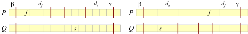
Figure A.1: An illustration of changes of tight slots and segments in Case (b1) of Lemma A.2 on the left and in Case (b2) on the right. The segments are separated by vertical dark-red line segments.

Proof.

We start by proving how the set of packets in the optimal plan changes. Let ${{\mathcal{U}}}$ be the set of packets pending before $s$ is released and ${{\mathcal{U}}}^{\prime}={{\mathcal{U}}}\cup{\left\{s\right\}}$ be the set of pending packets after the release of $s$. We consider two “parallel” runs of Algorithm ComputePlan, one on ${{\mathcal{U}}}$ to compute ${P}$ and the other on ${{\mathcal{U}}}^{\prime}$ to compute ${Q}$.

Suppose first that $w_{s}<w_{f}$. Then both runs will be identical until right after the time when $f$ is considered. Thus ${P}_{{\trianglerighteq{\hskip 0.5pt}}f}={Q}_{{\trianglerighteq{\hskip 0.5pt}}f}$. Moreover, as $f$ is the minimum-weight packet in ${P}$ with $d_{f}\leq\gamma=\textsf{nextts}({P},d_{s})$, we have ${P}[t,\gamma]\subseteq{P}_{{\trianglerighteq{\hskip 0.5pt}}f}$, that is, all packets in ${P}$ with deadline at most $\gamma$ are in ${P}_{{\trianglerighteq{\hskip 0.5pt}}f}$. Thus ${\textsf{pslack}}({Q}_{{\trianglerighteq{\hskip 0.5pt}}f},\gamma)={\textsf{pslack}}({P}_{{\trianglerighteq{\hskip 0.5pt}}f},\gamma)={\textsf{pslack}}({P},\gamma)=0$. Therefore, as $d_{s}\leq\gamma$ and as $s$ is considered after $f$, packet $s$ will not be admitted, which implies that both runs produce the same plan ${P}={Q}$.

For the rest of the proof, we assume that $w_{s}>w_{f}$. To prove that ${Q}={P}\cup{\left\{s\right\}}\setminus{\left\{f\right\}}$, based on Observation A.1(b), without loss of generality we can assume that $w_{s}=w_{f}+\varepsilon$ for a tiny $\varepsilon>0$, so that $s$ immediately precedes $f$ in the ordering of ${{\mathcal{U}}}^{\prime}$ by decreasing weights. Specifically, since $f\in{P}$, ${P}$ does not change if $f$’s weight is increased to $w_{s}-\varepsilon$. We will show that ${Q}={P}\cup{\left\{s\right\}}\setminus{\left\{f\right\}}$ with this increased weight of $f$. But as then $f\notin{Q}$, decreasing $f$’s weight back to its original value does not change $Q$.

With the assumption about $w_{f}$, the run on ${{\mathcal{U}}}^{\prime}$ before $s$ is considered will be identical to the run on ${{\mathcal{U}}}$ before $f$ is considered, thus ${Q}_{{\triangleright{\hskip 0.5pt}}s}={P}_{{\triangleright{\hskip 0.5pt}}f}$. In the next step of these runs, we consider packet $f$ for ${P}$ and $s$ for ${Q}$. We now have two cases.

Suppose that $d_{s}>d_{f}$. Then, since $f$ is admitted to ${P}$, we have ${\textsf{pslack}}({P}_{{\triangleright{\hskip 0.5pt}}f},\tau)\geq 1$ for $\tau\geq d_{f}$, which, by the paragraph above, implies that ${\textsf{pslack}}({Q}_{{\triangleright{\hskip 0.5pt}}s},\tau)\geq 1$ for $\tau\geq d_{s}$; and thus $s$ will be admitted to ${Q}$. As $d_{f},d_{s}\leq\gamma$, we also have ${\textsf{pslack}}({Q}_{{\trianglerighteq{\hskip 0.5pt}}s},\gamma)={\textsf{pslack}}({P}_{{\trianglerighteq{\hskip 0.5pt}}f},\gamma)=0$. This means that in the run on ${{\mathcal{U}}}^{\prime}$ packet $f$, which is considered next, will be rejected. From this point on, both runs are again the same, because no packet with deadline at most $\gamma$ is admitted, and because for $\tau>\gamma$ and any packet $g$ lighter than $f$ we have ${\textsf{pslack}}({P}_{{\triangleright{\hskip 0.5pt}}g},\tau)={\textsf{pslack}}({Q}_{{\triangleright{\hskip 0.5pt}}g},\tau)$, so $g$ gets admitted to ${Q}$ if and only if $g$ is admitted to ${P}$.

Next, consider the case when $d_{s}\leq d_{f}$. In this case, since also $d_{f}\leq\gamma$, we have $\textsf{nextts}({P},d_{f})=\gamma$, so the interval $(\beta,\gamma]$ is in fact a single segment of ${P}$. (This also proves the second claim in Case (b2), namely that $(\beta,\gamma]$ is a segment of ${P}$.) This gives us that ${\textsf{pslack}}({P}_{{\triangleright{\hskip 0.5pt}}f},\tau)\geq{\textsf{pslack}}({P},\tau)\geq 1$ for all $\tau\in(\beta,\gamma)$. Since ${P}$ admits $f$, we also have ${\textsf{pslack}}({P}_{{\triangleright{\hskip 0.5pt}}f},\tau)\geq 1$ for all $\tau\geq d_{f}$. Therefore ${\textsf{pslack}}({Q}_{{\triangleright{\hskip 0.5pt}}s},\tau)={\textsf{pslack}}({P}_{{\triangleright{\hskip 0.5pt}}f},\tau)\geq 1$ for all $\tau\geq d_{s}$, which implies that ${Q}$ will admit $s$. As in the previous case, we will then have ${\textsf{pslack}}({Q}_{{\trianglerighteq{\hskip 0.5pt}}s},\gamma)={\textsf{pslack}}({P}_{{\trianglerighteq{\hskip 0.5pt}}f},\gamma)=0$, so the run for ${Q}$ will not admit $f$ (which is next in the ordering), and the remainders of both runs will be identical.

Next, to prove parts (a)–(c) in the case $w_{s}>w_{f}$, we analyze the changes of ${\textsf{pslack}}()$ and ${\textsf{minwt}}()$ caused by the arrival of $s$.

(a) This part is straightforward, as replacing $f$ by $s$ in the plan does not change any value of $|{P}[t,\tau]|$ for slots $\tau\in[t,\min(d_{f},d_{s}))\cup[\max(d_{f},d_{s}),{T}]$. In particular, $\beta$ and $\gamma$ remain tight in ${Q}$, and slots in $(\beta,\min(d_{f},d_{s}))\cup[\max(d_{f},d_{s}),\gamma)$ are not tight in ${Q}$.

(b) Recall that ${Q}={P}\cup{\left\{s\right\}}\setminus{\left\{f\right\}}$. Suppose that $d_{s}>d_{f}$. Then ${\textsf{pslack}}({Q},\tau)={\textsf{pslack}}({P},\tau)+1$ for $\tau\in[d_{f},d_{s})$ as $|{Q}[t,\tau]|=|{P}[t,\tau]|-1$ for such $\tau$. So there are no tight slots in the interval $[d_{f},d_{s})$ in ${Q}$. This shows (b1).

The argument for (b2) is similar. Suppose that $d_{s}\leq d_{f}$. As already justified earlier, $(\beta,\gamma]$ is a segment of ${P}$. Hence, as $\beta<d_{s}\leq d_{f}\leq\gamma$, the slack values for $\tau\in[d_{s},d_{f})$ are strictly positive in ${P}$. Further, ${\textsf{pslack}}({Q},\tau)={\textsf{pslack}}({P},\tau)-1\geq 0$ for $\tau\in[d_{s},d_{f})$. This means that in ${Q}$ there may appear additional tight slots in $[d_{s},d_{f})$.

(c) For $\tau\in[t,\beta]$, the set of packets with deadline at most $\tau$ does not change and tight slots up to $\beta$ remain the same. Hence, ${\textsf{minwt}}({Q},\tau)={\textsf{minwt}}({P},\tau)$ for such $\tau$. For $\tau\in(\beta,\gamma]$, it holds that ${\textsf{minwt}}({P},\tau)=w_{f}$ and, as $s$ replaces $f$ and $\gamma$ remains a tight slot, all packets in ${Q}$ with deadlines at most $\textsf{nextts}({Q},\tau)\leq\gamma$ are heavier than $f$, so we actually have ${\textsf{minwt}}({Q},\tau)>{\textsf{minwt}}({P},\tau)$. Finally, consider $\tau>\gamma$. Since tight slots after $\gamma$ are unchanged, the set of packets considered in the definition of ${\textsf{minwt}}(\tau)$ changes only by replacing $f$ by $s$ with $w_{s}>w_{f}$, which implies ${\textsf{minwt}}({Q},\tau)\geq{\textsf{minwt}}({P},\tau)$. ∎

The observation below provides a characterization of optimal plans in terms of the ${\textsf{minwt}}()$ function. Its $(\Rightarrow)$ implication follows from the first claim of Lemma A.2. The $(\Leftarrow)$ implication follows by noting that if a plan ${P}$ satisfies the condition in the observation then running Algorithm ComputePlan on ${{\mathcal{U}}}$ will produce exactly the set of packets in ${P}$. (The formal proof proceeds by induction, showing that packets from ${P}$ will be admitted to $X$ because ${P}$ is feasible, but packets from ${{\mathcal{U}}}\setminus{P}$ will not, as the condition in line (4) will be violated at the time they are considered.)

Observation A.3.

A plan ${P}$ is optimal for a set ${{\mathcal{U}}}$ of pending packets if and only if $w_{j}<{\textsf{minwt}}({P},d_{j})$ for all packets $j\in{{\mathcal{U}}}\setminus{P}$.

A.2 Updating the Optimal Plan after Transmitting a Packet

Next, we analyze how the optimal plan evolves after an algorithm transmits a packet from the current optimal plan. (Only such transmissions are relevant to our analysis as in our algorithm PlanM packets from outside the optimal plan are not considered for transmission.) We stress that in this section we only analyze the effects of the event of a packet being transmitted, and the properties we establish are independent of the algorithm. In Appendix B we will deal with the changes in the plan specific to PlanM, namely with packet transmissions that also involve adjustments of the instance.

So let ${{\mathcal{U}}}$ be the set of packets pending at a time $t$ and denote by ${P}={P}^{t}$ the optimal plan for ${{\mathcal{U}}}$. Suppose that we choose some packet $p\in{P}$, transmit it at time $t$, and advance the time to $t+1$. The set ${{\mathcal{U}}}^{\prime}$ of packets pending at time $t+1$ is obtained from ${{\mathcal{U}}}$ by removing $p$ and all packets that expire at time $t$. In this section, ${Q}$ will denote the new optimal plan for ${{\mathcal{U}}}^{\prime}$ and time step $t+1$; that is ${Q}={\widetilde{{P}}}^{t+1}$ in the notation from Section 5.5.

We now explain how to obtain ${Q}$ from ${P}$. There are two cases, depending on whether or not $p$ is in the initial segment $[t,\alpha]$ of ${P}$, where $\alpha=\textsf{nextts}({P},t)$. We start with the case when $p$ is in the initial segment, which is quite straightforward. See Figure A.2 for an illustration.

Lemma A.4.

(The Plan-Update Lemma for Transmitting $p\in{P}[t,\alpha]$.) Suppose that at time $t$ we transmit a packet $p\in{P}[t,\alpha]$, where $\alpha=\textsf{nextts}({P},t)$. Then:

1. ${Q}={P}\setminus{\left\{p\right\}}$. Thus the new optimal plan ${Q}$ is obtained from ${P}$ simply by removing $p$.

2. ${\textsf{pslack}}({Q},\tau)={\textsf{pslack}}({P},\tau)-1$ for $\tau\in[t+1,d_{p})$ and ${\textsf{pslack}}({Q},\tau)={\textsf{pslack}}({P},\tau)$ for $\tau\geq d_{p}$. Thus new tight slots may appear in $[t+1,d_{p})$.

3. For any slot $\tau\geq t+1$, ${\textsf{minwt}}({Q},\tau)\geq{\textsf{minwt}}({P},\tau)$.

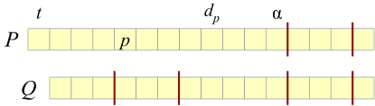
Figure A.2: An illustration of changes of tight slots and segments in Lemma A.4.

Note that part (b) is meaningful in the special case when $d_{p}=t$, as according to our definition of ${\textsf{pslack}}()$, ${\textsf{pslack}}({Q},t)$ is defined and equal to $0$, that is slot $t$ is considered tight at time $t+1$.

Proof.

Observe first that ${P}\setminus{\left\{p\right\}}\subseteq{{\mathcal{U}}}^{\prime}$. Indeed, if some $q\in{P}\setminus{\left\{p\right\}}$ had $d_{q}=t$, it would mean that the first tight slot $\alpha$ is $t$, so $q$ would have to be equal to $p$.

(a) According to Observation A.1(c), ${P}$ has a schedule where $p$ is scheduled in slot $t$. This implies directly that ${P}\setminus{\left\{p\right\}}$ is a feasible set of packets at time $t+1$. If ${Q}^{\prime}\neq{P}\setminus{\left\{p\right\}}$ is any other feasible subset of ${{\mathcal{U}}}^{\prime}$ then ${Q}^{\prime}$ would have a schedule starting at time $t+1$, so ${P}^{\prime}={Q}^{\prime}\cup{\left\{p\right\}}$ would have a schedule starting at time $t$, and thus would be feasible at time $t$. Since ${P}$ is heavier than ${P}^{\prime}$, ${P}\setminus{\left\{p\right\}}$ is heavier than ${Q}^{\prime}$; thus proving that the optimal plan at time $t+1$ is indeed ${Q}={P}\setminus{\left\{p\right\}}$.

(b) For $\tau\in[t+1,d_{p})$, ${\textsf{pslack}}({Q},\tau)={\textsf{pslack}}({P},\tau)-1$ as in ${Q}$ the time is incremented and $|{Q}[t+1,\tau]|=|{P}[t+1,\tau]|$. For $\tau\geq d_{p}$, incrementing the time for ${Q}$ is compensated by $p$ not contributing to ${Q}[t+1,\tau]$ (that is $|{Q}[t+1,\tau]|=|{P}[t+1,\tau]|-1$), and thus ${\textsf{pslack}}({Q},\tau)={\textsf{pslack}}({P},\tau)$.

(c) By (b), the value of $\textsf{nextts}({P},\tau)$ may only decrease. Since also no packet is added to the plan, in the definition of ${\textsf{minwt}}({Q},\tau)$ we consider a subset of packets used to define ${\textsf{minwt}}({P},\tau)$, which shows (c). ∎

For the case $p\in{P}(\alpha,{T}]$, recall that the substitute packet $\textsf{sub}({P},p)$ for $p$ is the heaviest pending packet $\varrho\in{{\mathcal{U}}}\setminus{P}$ satisfying $d_{\varrho}>\textsf{prevts}({P},d_{p})$. We prove that $\textsf{sub}({P},p)$ really appears in the plan when $p$ is transmitted. See Figure A.3 for an illustration.

Lemma A.5.

(The Plan-Update Lemma for Transmitting $p\ \in{P}(\alpha,{T}]$.) Suppose that at time $t$ we transmit a packet $p\in{P}(\alpha,{T}]$, where $\alpha=\textsf{nextts}({P},t)$. Let $\varrho=\textsf{sub}({P},p)$, $\beta=\textsf{prevts}({P},d_{p})$, $\gamma=\textsf{nextts}({P},d_{\varrho})$, and denote by ${\ell}$ the lightest packet in ${P}[t,\alpha]$, i.e., in the initial segment of ${P}$. Then:

1. ${Q}={P}\setminus{\left\{p,{\ell}\right\}}\cup{\left\{\varrho\right\}}$. Thus the new optimal plan ${Q}$ is obtained from ${P}$ by removing ${\ell}$ and replacing $p$ by $\varrho$.

2. ${\textsf{pslack}}({Q},\tau)={\textsf{pslack}}({P},\tau)-1$ for $\tau\in[t+1,d_{\ell})$.

3. ${\textsf{pslack}}({Q},\tau)={\textsf{pslack}}({P},\tau)$ for $\tau\in[d_{\ell},\min(d_{p},d_{\varrho}))\cup[\max(d_{p},d_{\varrho}),{T}]$.

4. For $\tau\in[\min(d_{p},d_{\varrho}),\max(d_{p},d_{\varrho}))$ there are two cases:

   1. If $d_{\varrho}>d_{p}$, then ${\textsf{pslack}}({Q},\tau)={\textsf{pslack}}({P},\tau)+1$ for $\tau\in[d_{p},d_{\varrho})$. This means that all segments of ${P}$ in $(\beta,\gamma]$ get merged into one segment $(\beta,\gamma]$ of ${Q}$.

   2. If $d_{\varrho}<d_{p}$, then ${\textsf{pslack}}({Q},\tau)={\textsf{pslack}}({P},\tau)-1$ for $\tau\in[d_{\varrho},d_{p})$. In this case $(\beta,\gamma]$ is itself a segment of ${P}$, and in ${Q}$ there might be new tight slots in $[d_{\varrho},d_{p})$ that partition $(\beta,\gamma]$ into smaller segments.

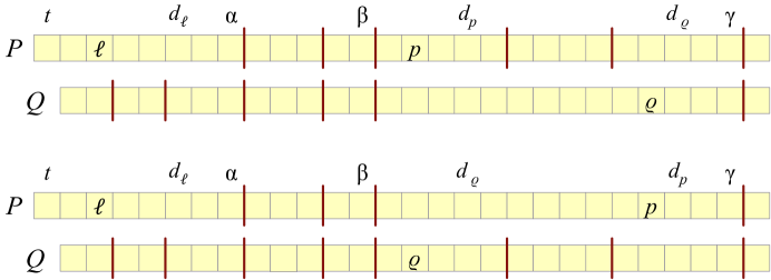
Figure A.3: An illustration of changes of tight slots and segments, in Case (d1) of Lemma A.5 on the top and in Case (d2) on the bottom.

Proof.

(a) Let ${{\mathcal{U}}}$ be the set of packets pending at time $t$ before transmitting $p$ and ${{\mathcal{U}}}^{\prime}$ be the packets that remain pending at time $t+1$ after $p$ is transmitted; that is, ${{\mathcal{U}}}^{\prime}$ is obtained from ${{\mathcal{U}}}$ by removing $p$ and all packets that expire at time $t$. We observe first that ${P}\setminus{\left\{p,{\ell}\right\}}\subseteq{{\mathcal{U}}}^{\prime}$. Indeed, if there was some $q\in{P}\setminus{\left\{p,{\ell}\right\}}$ with $d_{q}=t$, this would imply that $\alpha=t$, so $d_{\ell}=t$ and thus ${\ell}=q$, contradicting the choice of $q$. Obviously, $p\notin{{\mathcal{U}}}^{\prime}$. As for ${\ell}$, it may or may not be in ${{\mathcal{U}}}^{\prime}$, depending on whether or not $d_{\ell}>t$. We also have $\varrho\in{{\mathcal{U}}}^{\prime}$, because $d_{\varrho}>\beta\geq t$.

We prove that ${Q}={P}\setminus{\left\{p,{\ell}\right\}}\cup{\left\{\varrho\right\}}$ in two substeps:

• First, we increment the time to $t+1$ but without transmitting $p$. After this substep the set of pending packets is ${\overline{{\mathcal{U}}}}={\left\{a\in{{\mathcal{U}}}{\;:\;}d_{a}\geq t+1\right\}}$, i.e., we exclude packets that expire at time $t$. We show that the optimal plan for ${\overline{{\mathcal{U}}}}$ is ${\overline{{Q}}}={P}\setminus{\left\{{\ell}\right\}}$.

• In the second substep we remove $p$ from ${\overline{{\mathcal{U}}}}$ (and transmit it in time slot $t$), so the new set of pending packets will be ${{\mathcal{U}}}^{\prime}={\overline{{\mathcal{U}}}}\setminus{\left\{p\right\}}$, and we prove that the new optimal plan will be ${Q}={\overline{{Q}}}\setminus{\left\{p\right\}}\cup{\left\{\varrho\right\}}$. (Recall that we have $p\neq{\ell}$ as $p\not\in{P}[t,\alpha]$ and ${\ell}\in{P}[t,\alpha]$.)

The intuition is that these two substeps are largely independent: incrementing $t$ to $t+1$ will squeeze out ${\ell}$ from ${P}$, no matter what packets with deadlines after $\alpha$ are removed from ${{\mathcal{U}}}$.

First substep. For the first substep, we use an argument similar to the one in Lemma A.4. Observe that ${P}\setminus{\left\{{\ell}\right\}}$ is a feasible set of packets at time $t+1$, since ${P}$ has a schedule where ${\ell}$ is in slot $t$, by Observation A.1(c). Let ${Q}^{\prime}\neq{P}\setminus{\left\{{\ell}\right\}}$ be any other subset of ${\overline{{\mathcal{U}}}}$ that is feasible at time $t+1$; we show that $w({Q}^{\prime})<w({P}\setminus{\left\{{\ell}\right\}})$. Since ${P}$ contains exactly $\alpha-t+1$ packets with deadline at most $\alpha$, there is a packet $q^{\prime}\in{P}[t,\alpha]$ such that $q^{\prime}\notin{Q}^{\prime}$ (possibly $q^{\prime}={\ell}$). As ${Q}^{\prime}$ has a schedule starting at time $t+1$, ${P}^{\prime}={Q}^{\prime}\cup{\left\{q^{\prime}\right\}}$ has a schedule starting at time $t$ and thus is feasible at time $t$. Since ${P}$ is at least as heavy as ${P}^{\prime}$ and ${\ell}$ is the lightest packet in ${P}[t,\alpha]$, implying $w_{\ell}\leq w_{q^{\prime}}$, we conclude that indeed $w({P}\setminus{\left\{{\ell}\right\}})\geq w({Q}^{\prime})$. Hence, the plan after incrementing the time is indeed ${\overline{{Q}}}={P}\setminus{\left\{{\ell}\right\}}$.

Thus we can think of ${\overline{{Q}}}$ as being obtained from ${P}$ by advancing the time to $t+1$ and removing ${\ell}$. It follows that ${\textsf{pslack}}({\overline{{Q}}},\tau)={\textsf{pslack}}({P},\tau)$ for $\tau\geq d_{\ell}$. In particular, $\beta$ is a tight slot of ${\overline{{Q}}}$ and $\beta=\textsf{prevts}({\overline{{Q}}},d_{p})$. Further, as ${{\mathcal{U}}}$ and ${\overline{{\mathcal{U}}}}$ contain the same packets with deadline after $\beta$ and as $\beta\geq d_{\ell}$, we get that $\varrho$ is the heaviest packet in ${\overline{{\mathcal{U}}}}\setminus{\overline{{Q}}}$ with deadline greater than $\beta$. Summarizing, we have

$$\beta\; =\;\textsf{prevts}({\overline{{Q}}},d_{p})$$ (A.1)

$$\varrho\; =\;{\textrm{argmax}}_{j}{\left\{w_{j}{\;:\;}j\in{\overline{{\mathcal{U}}}}\setminus{\overline{{Q}}}\;\&\;d_{j}>\beta\right\}}$$ (A.2)

$$\gamma\; =\;\textsf{nextts}({\overline{{Q}}},d_{\varrho})$$ (A.3)

Second substep. In the second substep we establish a relationship between ${\overline{{Q}}}$ and ${Q}$. To this end, we consider two “parallel” runs of the greedy algorithm to compute plans: one run of ${\textsf{ComputePlan}}({\overline{{\mathcal{U}}}},t+1)$ which yields ${\overline{{Q}}}$ and another run of ${\textsf{ComputePlan}}({{\mathcal{U}}}^{\prime},t+1)$ which yields ${Q}$. (Recall that ${{\mathcal{U}}}^{\prime}={\overline{{\mathcal{U}}}}\setminus{\left\{p\right\}}$.) The contents of the set $X$ in these two runs after processing packets heavier than some packet $j$ is equal to ${\overline{{Q}}}_{{\triangleright{\hskip 0.5pt}}j}$ and ${{Q}}_{{\triangleright{\hskip 0.5pt}}j}$, respectively. To avoid ambiguity, we will be using these notations when referring to the contents of $X$ during these runs.

We divide these two runs into three phases. In the first phase we consider the two runs for packets $j$ with $w_{j}>w_{p}$ (that is, before $p$ gets admitted to ${\overline{{Q}}}$). Since ${\overline{{\mathcal{U}}}}_{{\triangleright{\hskip 0.5pt}}p}={{\mathcal{U}}}^{\prime}_{{\triangleright{\hskip 0.5pt}}p}$, in this phase the two runs are exactly the same. This gives us that

$${\overline{{Q}}}_{{\triangleright{\hskip 0.5pt}}p}\;=\;{Q}_{{\triangleright{\hskip 0.5pt}}p}.$$

The second phase involves packets $j$ with $w_{p}\geq w_{j}>w_{\varrho}$. We claim that during this phase the following invariants will be maintained:

$${Q}_{{\trianglerighteq{\hskip 0.5pt}}j}\; =\;{{\overline{{Q}}}}_{{\trianglerighteq{\hskip 0.5pt}}j}\setminus{\left\{p\right\}}$$ (A.4)

$${\textsf{pslack}}({Q}_{{\trianglerighteq{\hskip 0.5pt}}j},\tau)\; =\;\begin{cases}{\textsf{pslack}}({\overline{{Q}}}_{{\trianglerighteq{\hskip 0.5pt}}j},\tau)&\quad\text{for }\tau\in[t+1,\beta]\\ {\textsf{pslack}}({\overline{{Q}}}_{{\trianglerighteq{\hskip 0.5pt}}j},\tau)\geq 1&\quad\text{for }\tau\in(\beta,d_{p})\\ {\textsf{pslack}}({\overline{{Q}}}_{{\trianglerighteq{\hskip 0.5pt}}j},\tau)+1&\quad\text{for }\tau\geq d_{p}\\ \end{cases}$$ (A.5)

We first show that these properties hold for $j=p$. We have $p\in{\overline{{Q}}}$ and ${{\mathcal{U}}}^{\prime}={\overline{{\mathcal{U}}}}\setminus{\left\{p\right\}}$; this means that $p$ will be admitted to ${\overline{{Q}}}_{{\trianglerighteq{\hskip 0.5pt}}p}$ in the run for ${\overline{{\mathcal{U}}}}$ but it will not be considered in the run for ${{\mathcal{U}}}^{\prime}$. Thus Property (A.4) follows. Invariant (A.4) and the definition of ${\textsf{pslack}}()$ imply all relations between ${\textsf{pslack}}({Q}_{{\trianglerighteq{\hskip 0.5pt}}p},\tau)$ and ${\textsf{pslack}}({\overline{{Q}}}_{{\trianglerighteq{\hskip 0.5pt}}p},\tau)$ in invariant (A.5), and the inequality ${\textsf{pslack}}({\overline{{Q}}}_{{\trianglerighteq{\hskip 0.5pt}}p},\tau)\geq 1$ for $\tau\in(\beta,d_{p})$ follows immediately from (A.1). (Note that ${\textsf{pslack}}({\overline{{Q}}}_{{\trianglerighteq{\hskip 0.5pt}}a},\tau)\geq{\textsf{pslack}}({\overline{{Q}}},\tau)$ holds for any packet $a$ and slot $\tau$.)

Next, consider packets $j$ with $w_{p}>w_{j}>w_{\varrho}$. If $j$ gets admitted to ${\overline{{Q}}}_{{\trianglerighteq{\hskip 0.5pt}}j}$ then invariant (A.5) implies that it also gets admitted to ${{Q}}_{{\trianglerighteq{\hskip 0.5pt}}j}$, preserving (A.4). That (A.5) is preserved follows from the same argument as for $j=p$ above.

So consider the second case, when $j$ does not get admitted to ${\overline{{Q}}}_{{\trianglerighteq{\hskip 0.5pt}}j}$. We claim that $j$ will also not be admitted to ${{Q}}_{{\trianglerighteq{\hskip 0.5pt}}j}$. To justify this, we argue as follows. By (A.2), $\varrho$ is the heaviest packet in ${\overline{{\mathcal{U}}}}$ with deadline after $\beta$ that will not be admitted to ${\overline{{Q}}}$. Therefore, since $w_{j}>w_{\varrho}$, we have $d_{j}\leq\beta$. Suppose for a contradiction that $j$ is admitted to ${{Q}}_{{\trianglerighteq{\hskip 0.5pt}}j}$. As $j$ is not admitted to ${\overline{{Q}}}_{{\trianglerighteq{\hskip 0.5pt}}j}$, there must be $\tau\geq d_{j}$ such that ${\textsf{pslack}}({\overline{{Q}}}_{{\triangleright{\hskip 0.5pt}}j},\tau)=0$, although ${\textsf{pslack}}({Q}_{{\triangleright{\hskip 0.5pt}}j},\tau)>0$ as $j$ is admitted to ${{Q}}_{{\trianglerighteq{\hskip 0.5pt}}j}$. Due to invariant (A.5) for $\tau\in[t+1,\beta]$, we must have $\tau>\beta$. As $\tau$ is already tight, by Observation A.1(d) we get that ${\textsf{pslack}}({\overline{{Q}}}_{{\triangleright{\hskip 0.5pt}}j},\beta)={\textsf{pslack}}({\overline{{Q}}},\beta)=0$, where the second step holds by (A.1). Using invariant (A.5) for $\tau\in[t+1,\beta]$, we obtain ${\textsf{pslack}}({Q}_{{\triangleright{\hskip 0.5pt}}j},\beta)={\textsf{pslack}}({\overline{{Q}}}_{{\triangleright{\hskip 0.5pt}}j},\beta)=0$, contradicting that we must have ${\textsf{pslack}}({Q}_{{\triangleright{\hskip 0.5pt}}j},\beta)>0$ as $j$ is admitted to ${{Q}}_{{\trianglerighteq{\hskip 0.5pt}}j}$ and $d_{j}\leq\beta$. Thus we indeed have that $j$ will not be admitted to ${{Q}}_{{\trianglerighteq{\hskip 0.5pt}}j}$. As in this case $j$ is not admitted to both ${\overline{{Q}}}_{{\trianglerighteq{\hskip 0.5pt}}j}$ and ${{Q}}_{{\trianglerighteq{\hskip 0.5pt}}j}$, both invariants (A.4) and (A.5) are obviously preserved.

In the third phase we analyze both runs for packets $j$ with $w_{j}\leq w_{\varrho}$. We claim that for these packets the following invariants hold:

$${Q}_{{\trianglerighteq{\hskip 0.5pt}}j}\; =\;{{\overline{{Q}}}}_{{\trianglerighteq{\hskip 0.5pt}}j}\setminus{\left\{p\right\}}\cup{\left\{\varrho\right\}}$$ (A.6)

$${\textsf{pslack}}({Q}_{{\trianglerighteq{\hskip 0.5pt}}j},\tau)\; =\;{\textsf{pslack}}({\overline{{Q}}}_{{\trianglerighteq{\hskip 0.5pt}}j},\tau)\quad\text{for }\tau\geq\gamma$$ (A.7)

$${\textsf{pslack}}({Q}_{{\trianglerighteq{\hskip 0.5pt}}j},\gamma)\; =\;{\textsf{pslack}}({\overline{{Q}}}_{{\trianglerighteq{\hskip 0.5pt}}j},\gamma)\;=\;0$$ (A.8)

Note that property (A.7) follows directly from (A.6), because $d_{p},d_{\varrho}\leq\gamma$. Thus we only need to show that (A.6) and (A.8) hold for all $j$ in this phase.

We first consider $j=\varrho$. As $\varrho\notin{\overline{{Q}}}$, $\varrho$ will not be admitted to ${\overline{{Q}}}_{{\trianglerighteq{\hskip 0.5pt}}\varrho}$. From (A.5) and (A.2) we have that ${\textsf{pslack}}({Q}_{{\triangleright{\hskip 0.5pt}}\varrho},\tau)\geq 1$ for $\tau\geq d_{\varrho}$, and thus $\varrho$ will be admitted to ${Q}_{{\trianglerighteq{\hskip 0.5pt}}\varrho}$. This gives us (A.6) and (A.7). Since $\varrho\notin{\overline{{Q}}}$, all packets in ${\overline{{Q}}}[t+1,\gamma]$ are heavier than $\varrho$; in other words, we have ${\overline{{Q}}}[t+1,\gamma]={\overline{{Q}}}_{{\trianglerighteq{\hskip 0.5pt}}\varrho}[t+1,\gamma]$, which together with (A.3) implies that $\gamma=\textsf{nextts}({\overline{{Q}}}_{{\trianglerighteq{\hskip 0.5pt}}\varrho},d_{\varrho})$. Then, from (A.7) (that we already established for $\varrho$), we obtain that ${\textsf{pslack}}({Q}_{{\trianglerighteq{\hskip 0.5pt}}\varrho},\gamma)={\textsf{pslack}}({\overline{{Q}}}_{{\trianglerighteq{\hskip 0.5pt}}\varrho},\gamma)=0$.

In the rest of the third phase, for each packet $j$ with $w_{j}<w_{\varrho}$, condition (A.8) implies that if $d_{j}\leq\gamma$ then $j$ will not be admitted to ${\overline{{Q}}}_{{\trianglerighteq{\hskip 0.5pt}}j}$ and also to ${Q}_{{\trianglerighteq{\hskip 0.5pt}}j}$. On the other hand, if $d_{j}>\gamma$, then condition (A.7) implies that $j$ will be either admitted to both ${\overline{{Q}}}_{{\trianglerighteq{\hskip 0.5pt}}j}$ and ${Q}_{{\trianglerighteq{\hskip 0.5pt}}j}$ or to none. This completes the proof that the above invariants are preserved, and the proof of (a) as well.

(b) We now analyze the changes in the values of ${\textsf{pslack}}()$. If $d_{\ell}>t$, it holds that ${\textsf{pslack}}({Q},\tau)={\textsf{pslack}}({P},\tau)-1$ for $\tau\in[t+1,d_{\ell})$, as in the transmission step the time was incremented and there is no change in the set of packets taken into account.

(c) For $\tau\in[d_{\ell},\min(d_{\varrho},d_{p}))$ we have ${\textsf{pslack}}({Q},\tau)={\textsf{pslack}}({P},\tau)$ as in the transmission step the time was incremented, but ${\ell}$ was forced out. (In particular, since $d_{\ell}\leq\alpha<\min(d_{\varrho},d_{p})$, $\alpha$ is a tight slot in ${Q}$, including the special case when $\alpha=t$.) Similarly, for $\tau\geq\max(d_{\varrho},d_{p})$, it holds that ${\textsf{pslack}}({Q},\tau)={\textsf{pslack}}({P},\tau)$, since in the transmission step the time was incremented, ${\ell}$ was forced out, $p$ was transmitted, and $\varrho$ appeared in ${Q}$.

(d) In Case (d1), for $\tau\in[d_{p},d_{\varrho})$, we have ${\textsf{pslack}}({Q},\tau)={\textsf{pslack}}({P},\tau)+1$ as in the transmission step the time was increased, but ${\ell}$ was forced out and $p$ was transmitted. It follows that ${Q}$ has no tight slots in $[d_{p},d_{\varrho})$, so $\textsf{prevts}({Q},d_{\varrho})=\beta$ and $\textsf{nextts}({Q},d_{p})=\gamma$, which means that in ${Q}$ the interval $(\beta,\gamma]$ forms one segment.

In Case (d2), the definitions of $\beta=\textsf{prevts}({P},d_{p})$ and $\gamma=\textsf{nextts}({P},d_{\varrho})$, together with $d_{\varrho}<d_{p}$, imply that $(\beta,\gamma]$ is indeed a segment of ${P}$. In particular, this means that ${\textsf{pslack}}({P},\tau)\geq 1$ for $\tau\in[d_{\varrho},d_{p})$. For such slots $\tau$ we thus obtain that ${\textsf{pslack}}({Q},\tau)={\textsf{pslack}}({P},\tau)-1$ because in the transmission step the time was increased, ${\ell}$ was forced out, and $\varrho$ was added to ${Q}$. ∎

Note that after transmitting $p\in{P}(\alpha,{T}]$ (without adjusting packet weights or deadlines appropriately), the slot monotonicity property does not hold. This is because ${\textsf{minwt}}(d_{\varrho})$ decreases, as ${\textsf{minwt}}({P},d_{\varrho})>w_{\varrho}$ but ${\textsf{minwt}}({Q},d_{\varrho})=w_{\varrho}$.

Appendix B Appendix: Leap Step of Algorithm PlanM

Algorithm PlanM artificially adjusts weights and deadlines of some pending packets in leap steps, and therefore the results from the previous section are not sufficient to fully characterize how the optimal plan evolves during its computation. Lemmas A.2 and A.4 remain valid for Algorithm PlanM, but we still need a variant of Lemma A.5 that will characterize the changes in the optimal plan after a leap step. We provide such a characterization below, see Lemma B.1. Then we use this lemma to prove Lemma B.2, the slot-monotonicity property for leap steps.

In the following, similar to the previous section, we use ${P}$ for ${P}^{t}$ (the optimal plan after all packets at time $t$ have been released) and by ${Q}={\widetilde{{P}}}^{t+1}$ we denote the optimal plan just after the event of transmitting $p$, incrementing the time, and changing weights and deadlines (but before new packets at time $t+1$ are released).

Lemma B.1.

Suppose that $t$ is a leap step of Algorithm PlanM in which $p$ was transmitted, and let $\varrho=\textsf{sub}({P},p)$ be the substitute packet of $p$. Let packets $h_{0}=p,h_{1},\dots,h_{k}$ and tight slots $\tau_{0},\dots,\tau_{k}=\gamma=\textsf{nextts}({P},d^{t}_{\varrho})$ be as defined in the algorithm. Furthermore, let $\beta=\tau_{-1}=\textsf{prevts}({P},d^{t}_{p})$. Then:

1. ${Q}={P}\setminus{\left\{p,{\ell}\right\}}\cup{\left\{\varrho\right\}}$; in particular, if $k\geq 1$, all packets $h_{1},h_{2},\dots,h_{k}$ are in ${Q}$.

2. $w^{t}_{p}=w^{t}_{h_{0}}>w^{t}_{h_{1}}>w^{t}_{h_{2}}>\cdots>w^{t}_{h_{k}}>w^{t}_{\varrho}$.

3. $h_{k}$’s deadline is in the segment of ${P}$ ending at $\gamma$, that is, $\textsf{prevts}({P},d^{t}_{\varrho})<d^{t}_{h_{k}}\leq\gamma$.

4. The ${\textsf{pslack}}()$ values change as follows (see Figure B.1):

   1. ${\textsf{pslack}}({Q},\tau)={\textsf{pslack}}({P},\tau)-1$ for $\tau\in[t+1,d^{t}_{\ell})$.

   2. ${\textsf{pslack}}({Q},\tau)={\textsf{pslack}}({P},\tau)$ for $\tau\in[d^{t}_{\ell},\beta]$.

   3. If $k\geq 1$, then for $i=0,\dots,k-1$ we have the following changes in $(\tau_{i-1},\tau_{i}]$:

      1. ${\textsf{pslack}}({Q},\tau)={\textsf{pslack}}({P},\tau)$ for $\tau\in(\tau_{i-1},d^{t}_{h_{i}})\cup{\left\{\tau_{i}\right\}}$.

      2. ${\textsf{pslack}}({Q},\tau)={\textsf{pslack}}({P},\tau)+1$ for $\tau\in[d^{t}_{h_{i}},\tau_{i})$.

   4. ${\textsf{pslack}}({Q},\tau)={\textsf{pslack}}({P},\tau)$ for $\tau\in(\tau_{k-1},\min(d^{t}_{h_{k}},d^{t}_{\varrho}))$.

   5. For $\tau\in[\min(d^{t}_{h_{k}},d^{t}_{\varrho}),\max(d^{t}_{h_{k}},d^{t}_{\varrho}))$, there are two cases:

      1. If $d^{t}_{h_{k}}<d^{t}_{\varrho}$, then ${\textsf{pslack}}({Q},\tau)={\textsf{pslack}}({P},\tau)+1$ for $\tau\in[d^{t}_{h_{k}},d^{t}_{\varrho})$.

      2. If $d^{t}_{\varrho}<d^{t}_{h_{k}}$, then ${\textsf{pslack}}({Q},\tau)={\textsf{pslack}}({P},\tau)-1$ for $\tau\in[d^{t}_{\varrho},d^{t}_{h_{k}})$.

   6. ${\textsf{pslack}}({Q},\tau)={\textsf{pslack}}({P},\tau)$ for $\tau\geq\max(d^{t}_{h_{k}},d^{t}_{\varrho})$.

5. Any tight slot of ${P}$ is a tight slot of ${Q}$, but there might be new tight slots of ${Q}$ in $[t+1,d^{t}_{\ell})$ and, in Case (d.v.2), also in $[d^{t}_{\varrho},d^{t}_{h_{k}})$. Thus, in general, we have $\textsf{nextts}({Q},\tau)\leq\textsf{nextts}({P},\tau)$ for all $\tau\geq t+1$.

6. $w^{t+1}_{h_{i}}\geq{\textsf{minwt}}({P},d^{t+1}_{h_{i}})$ for any $i=1,\dots,k$, and $w^{t+1}_{\varrho}\geq{\textsf{minwt}}({P},d^{t+1}_{\varrho})$.

Proof.

(a) The claim clearly holds for a simple leap step by Lemma A.5, i.e., when $k=0$, because in this case the algorithm does not decrease deadlines, and increasing the weight of $\varrho$ does not change the new optimal plan ${Q}$, by Observation A.1(b).

Thus consider an iterated leap step. Let $\overline{{Q}}$ be the optimal plan after $p$ is transmitted and the time is increased, but before the adjustment of weights and deadlines in line 11 of the algorithm is taken into account. From Lemma A.5 we have $\overline{{Q}}={P}\setminus{\left\{p,{\ell}\right\}}\cup{\left\{\varrho\right\}}$; in particular, packets $h_{1},h_{2},\dots,h_{k}$ are in $\overline{{Q}}$. Our goal is to prove that $\overline{{Q}}={Q}$.

By Observation A.1(b), increasing the weights of packets in the optimal plan cannot change the plan, so it is sufficient to show that the feasibility and optimality of the plan is not affected by the decrease of the deadlines of packets $h_{1},h_{2},\dots,h_{k}$.

By Lemma A.5, all segments of $\overline{{Q}}$ between $\beta=\textsf{prevts}({P},d^{t}_{p})$ and $\gamma=\textsf{nextts}({P},d^{t}_{\varrho})$ get merged into one, which means that ${\textsf{pslack}}(\overline{{Q}},\tau)\geq 1$ for any $\tau\in(\beta,\gamma)$. For $i=1,\dots,k$, decreasing the deadline of $h_{i}$ from $d^{t}_{h_{i}}$ to $d^{t+1}_{h_{i}}=\tau_{i-1}$ decreases ${\textsf{pslack}}(\overline{{Q}},\tau)$ by $1$ for $\tau\in[\tau_{i-1},d^{t}_{h_{i}})$. All $k$ intervals where these decreases occur are contained in $(\beta,\gamma)$ and, since $d^{t}_{h_{i}}\leq\tau_{i}$ for all $i$, these intervals do not overlap. Thus, after decreasing the deadlines of the $h_{i}$’s, all values of ${\textsf{pslack}}()$ will remain non-negative for $\overline{{Q}}$, so $\overline{{Q}}$ remains a feasible set of packets. Decreasing these deadlines cannot make previously unfeasible sets of packets feasible, implying that ${Q}$ remains optimal. Thus $\overline{{Q}}={Q}$, as claimed. In particular, packets $h_{1},h_{2},\dots,h_{k}$ remain in ${Q}$.

(b) By the choice of $p$ in the algorithm, $p$ is the heaviest packet in the segments of ${P}$ in $(\beta,\gamma]$, because $\varrho$ is the substitute packet for any packet in ${P}$ with deadline in $(\beta,\gamma]$. Thus for each $i=1,\dots,k$, since $d^{t}_{h_{i}}\in(\beta,\gamma]$, we get $w^{t}_{p}>w^{t}_{h_{i}}$. The ordering of weights of $h_{i}$’s follows from the definition of $h_{i}$’s in line 9 of the algorithm’s description. Finally, for any $i=0,\dots,k$ inequality $w^{t}_{h_{i}}>w^{t}_{\varrho}$ holds, because $\varrho\notin{P}$ and $d^{t}_{h_{i}}<\gamma=\textsf{nextts}({P},d^{t}_{\varrho})$.

(c) This holds by the definition of $h_{i}$’s in line 9 and by the condition of the while loop in line 7, which stops the loop when $\tau_{i}=\textsf{nextts}({P},d^{t}_{h_{i}})=\gamma$.

(d) For any slot $\tau\in[t+1,\beta]\cup(\gamma,{T}]$ the value of ${\textsf{pslack}}(\tau)$ is not affected by the decrease of the deadlines of $h_{i}$’s, since $h_{i}$’s are both in ${P}$ and in ${Q}$ and since their old and new deadlines are in $(\beta,\gamma]$. We thus get exactly the same changes of the ${\textsf{pslack}}()$ values outside $(\beta,\gamma]$ as in Lemma A.5. Regarding slots in $(\beta,\gamma]$, Lemma A.5(d) shows that ${\textsf{pslack}}(\tau)$ decreases by 1 for $\tau\in[d^{t}_{\varrho},d^{t}_{p})$ if $d^{t}_{\varrho}<d^{t}_{p}$, and increases by 1 for $\tau\in[d^{t}_{p},d^{t}_{\varrho})$ if $d^{t}_{p}<d^{t}_{\varrho}$. In the former case, we have $\tau_{0}=\gamma$ as $d^{t}_{\varrho}$ and $d^{t}_{p}$ are in the same segment, that is $k=0$. In the latter case, we sum the increase of values ${\textsf{pslack}}(\tau)$ for $\tau\in[d^{t}_{p},d^{t}_{\varrho})$ with the changes of the ${\textsf{pslack}}()$ values due to decreasing the deadlines of $h_{i}$’s, analyzed in (a), and we get the changes summarized in (d); see Figure B.1.

Part (e) follows from (c) and (d), which imply that the value of ${\textsf{pslack}}({P},\tau)$ does not increase for any tight slot $\tau$ in ${P}$.

Part (f) follows from the way the weights are changed in lines 4 and 11 of the algorithm. ∎

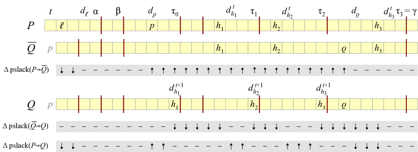
Figure B.1: An example with $k=3$ illustrating the proof of Lemma B.1(d), by showing changes of the ${\textsf{pslack}}()$ values in an iterated leap step. Here, notations $\Delta{\textsf{pslack}}({P}\rightarrow\overline{{Q}})$, $\Delta{\textsf{pslack}}(\overline{{Q}}\rightarrow{{Q}})$, and $\Delta{\textsf{pslack}}({P}\rightarrow{Q})$ represent the changes of the ${\textsf{pslack}}()$ in the two substeps (from ${P}$ to $\overline{{Q}}$ and from $\overline{{Q}}$ to ${{Q}}$), and the overall change from ${P}$ to ${Q}$, respectively. Up and down arrows represent increases and decreases of the values of ${\textsf{pslack}}()$ in individual slots.

Next, we show that, thanks to the deadline adjustments in Algorithm PlanM, the slot monotonicity property for optimal plans is preserved in leap steps.

Lemma B.2.

If step $t$ is a leap step of Algorithm PlanM, then ${\textsf{minwt}}({Q},\tau)\geq{\textsf{minwt}}({P},\tau)$ for any $\tau\geq t+1$.

Proof.

We use notation from Lemma B.1. By Lemma B.1(e) all tight slots of ${P}$ are tight slots of ${Q}$ (in particular, $\beta$ and $\gamma$ remain tight slots); thus $\textsf{nextts}({Q},\tau)\leq\textsf{nextts}({P},\tau)$ for all $\tau\geq t+1$. Fix some $\tau\geq t+1$, and let $a$ be the packet that realizes ${\textsf{minwt}}({Q},\tau)$, that is the minimum-weight packet in ${Q}$ with $d^{t+1}_{a}\leq\textsf{nextts}({Q},\tau)$. We need to show that $w^{t+1}_{a}\geq{\textsf{minwt}}({P},\tau)$. We have three cases.

Case 1: $\tau\leq\beta$. Lemma B.1(a) shows that ${\ell}$ is forced out of the optimal plan, thus not in ${Q}$, and otherwise the set of packets in the optimal plan with deadline at most $\beta$ does not change, that is, ${Q}[t+1,\beta]={P}[t,\beta]\setminus{\left\{{\ell}\right\}}$. It follows that $a\in{P}$ and its weight and deadline remain the same. We thus have $d^{t}_{a}=d^{t+1}_{a}\leq\textsf{nextts}({Q},\tau)\leq\textsf{nextts}({P},\tau)$, so $a$ is considered in the definition of ${\textsf{minwt}}({P},\tau)$, which implies $w^{t+1}_{a}=w^{t}_{a}\geq{\textsf{minwt}}({P},\tau)$.

Case 2: $\tau\in(\beta,\gamma]$. If $a\notin{\left\{h_{1},...,h_{k+1}\right\}}$ (in particular, this means that $a\neq\varrho=h_{k+1}$), then $a$ is also in ${P}$ with the same deadline and weight. As $\textsf{nextts}({Q},\tau)\leq\textsf{nextts}({P},\tau)$, we get $d^{t}_{a}\leq\textsf{nextts}({P},\tau)$, hence $w^{t+1}_{a}\geq{\textsf{minwt}}({P},\tau)$ follows as in Case 1.

Next, suppose that $a=h_{i}$ for some $i\in{\left\{1,\dots,k\right\}}$ (excluding the case $a=h_{k+1}=\varrho$). Recall that, as a result of changes in line 11 in the algorithm, we have $w^{t+1}_{a}\geq{\textsf{minwt}}({P},\tau_{i-1})$ and $d^{t+1}_{a}=\tau_{i-1}$. The definition of ${\textsf{minwt}}({Q},\tau)$ gives us that $\tau_{i-1}=d^{t+1}_{a}=\textsf{nextts}({Q},\tau)$, so $\tau>\textsf{prevts}({Q},\tau_{i-1})$. Thus, since tight slots of ${P}$ are tight also in ${Q}$, implying $\textsf{prevts}({Q},\tau_{i-1})\geq\textsf{prevts}({P},\tau_{i-1})$, we get that $\tau>\textsf{prevts}({P},\tau_{i-1})$. So $\tau$ is in the segment $(\textsf{prevts}({P},\tau_{i-1}),\tau_{i-1}]$ of $P$. By definition, for each segment of ${P}$ the value of ${\textsf{minwt}}({P},\tau^{\prime})$ is constant for all $\tau^{\prime}$ in this segment. Therefore ${\textsf{minwt}}({P},\tau_{i-1})={\textsf{minwt}}({P},\tau)$, and we conclude that $w^{t+1}_{a}\geq{\textsf{minwt}}({P},\tau_{i-1})={\textsf{minwt}}({P},\tau)$.

Finally, consider the case when $a=\varrho$. Recall that $w^{t+1}_{\varrho}={\textsf{minwt}}({P},d^{t}_{\varrho})$ and $d^{t}_{\varrho}=d^{t+1}_{\varrho}$. We have $\tau>\textsf{prevts}({Q},d^{t}_{\varrho})$, which implies that $\tau>\textsf{prevts}({P},d^{t}_{\varrho})=\textsf{prevts}({P},\gamma)$. Thus $\tau$ is in the segment $(\textsf{prevts}({P},\gamma),\gamma]$ of $P$, just like $\varrho$. It follows that $w^{t+1}_{\varrho}={\textsf{minwt}}({P},d^{t}_{\varrho})={\textsf{minwt}}({P},\tau)$.

Case 3: $\tau>\gamma$. The set of packets in the plan with deadline strictly after $\gamma$ does not change and also their weights and deadlines remain the same. Thus if $d^{t}_{a}>\gamma$, then using $\textsf{nextts}({Q},\tau)\leq\textsf{nextts}({P},\tau)$ again, we obtain that $w^{t+1}_{a}\geq{\textsf{minwt}}({P},\tau)$. Otherwise, $d^{t}_{a}\leq\gamma$, thus $w^{t+1}_{a}\geq{\textsf{minwt}}({Q},\gamma)\geq{\textsf{minwt}}({P},\gamma)\geq{\textsf{minwt}}({P},\tau)$, where the second inequality follows from Case 2 and the third one from $\gamma<\tau$. ∎

Appendix C Appendix: Simpler Variants of Algorithm PlanM

In this appendix, we provide some intuition on why the iterative choice of packets $h_{i}$ in Algorithm PlanM (line 9) is essentially needed in an iterated leap step. We first give an example of an instance showing that a memoryless variant of our algorithm does not achieve ratio $\phi$; this variant simply transmits packet $p$ according to Line 1 of Algorithm PlanM (and does not make any changes of packet weights and deadlines).

This memoryless algorithm does not maintain the slot-monotonicity property, so this still leaves open the possibility that perhaps some simpler way of maintaining this property is sufficient to achieve $\phi$-competitiveness. To address this, we further give an instance which shows a lower bound higher than $\phi$ on the competitive ratio of two simpler variants of Algorithm PlanM that maintain the slot-monotonicity property.

C.1 Counterexample for the Memoryless Variant of PlanM

The memoryless variant of Algorithm PlanM, denoted PlanM-Memoryless, is very simple: In each step $t$, transmit packet $p\in P^{t}$ that maximizes $w_{p}+\phi\cdot w(\textsf{sub}^{t}(p))$. That is, it chooses the packet for transmission in the same way as Algorithm PlanM, but it does not make any modifications of the instance. We now show that PlanM-Memoryless is not $\phi$-competitive.

Recall that slot-monotonicity is preserved if Algorithm PlanM executes a packet from the initial segment in each step (see Lemma A.4). For such instances, PlanM-Memoryless is equivalent to Algorithm PlanM and thus it achieves ratio $\phi$. Hence, a hard example for PlanM-Memoryless needs to involve some leap steps.

We give an example of an instance for which PlanM-Memoryless is not $\phi$-competitive. Our instance uses three interleaved infinite sequences of packets with weights increasing geometrically by factor $\phi^{2}$, similar to the examples in Section 4. These packets will now have span $4$. The basic idea is that the competitive ratio in each step (i.e., the ratio of the weights of packets transmitted by the optimum and by the algorithm) will be $\phi^{2}$ on these geometric sequences. In the example in Section 4, the online algorithm’s ratio on the geometric sequence is also $\phi^{2}$, but it can catch up with the optimum at the end, as in the last slots it still has some heavy packets pending that are not pending for the optimum. The trick behind our construction is to add several packets near the end that will force PlanM-Memoryless to make some leap steps in which these new packets will be transmitted, while the older packets will expire.

packet $q$	weight $w_{q}$
$\varrho$	$1-\epsilon$
$\varrho_{i}$	$\phi^{-2i}w_{\varrho}$
$x$	$1$
$x_{i}$	$\phi^{-2i}w_{x}$
$z$	$\phi$
$z_{i}$	$\phi^{-2i}w_{z}$
${\dot{z}}$	$\phi-\epsilon$
$s^{\prime}$	$2+2\epsilon$
$s$	$\phi^{2}+2\epsilon$
${\dot{x}}$	$1-\epsilon$
$\varrho^{\prime}$	$\phi^{-2}$
$e$	$\epsilon$

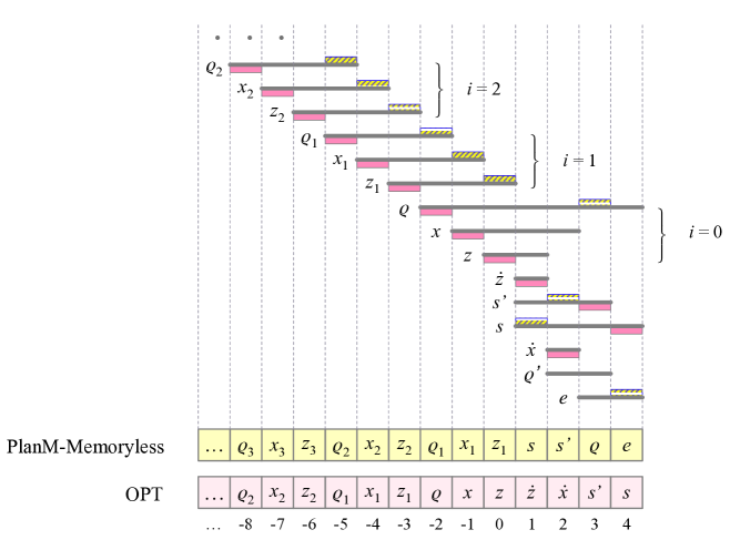
Figure C.1: An instance on which PlanM-Memoryless has ratio larger than $\phi$. The table on the left shows the weights, the figure on the right shows release times and deadlines. The figure also shows the schedules of PlanM-Memoryless and the optimal schedule. The schedules are outlined at the bottom, and they are also depicted using unit-width rectangles (pink for the optimum and yellow and striped for the algorithm) attached to the line segments representing packet spans.

The instance is defined in Figure C.1. To ensure consistent tie-breaking, we use a small parameter ${\epsilon}>0$ in packet weights. The three sequences of packets with span $4$ and geometrically increasing weights are ${\left\{\varrho_{i}\right\}}_{i=1}^{\infty}$, ${\left\{x_{i}\right\}}_{i=1}^{\infty}$ and ${\left\{z_{i}\right\}}_{i=1}^{\infty}$. When estimating profits, we will also include packets $\varrho_{0}=\varrho$, $x_{0}=x$, and $z_{0}=z$ in these sequences, even though the spans of $\varrho$ and $z$ are not equal to $4$. This figure also shows the schedule computed by PlanM-Memoryless and the optimal schedule. The steps of PlanM-Memoryless are explained below:

Steps $t=...,-2,-1,0$: As in the example in Section 4, when scheduling the packets in steps $t=...,-2,-1,0$, the algorithm will always transmit the packet that is tight at the given step. This is because at each step $t=...,-4,-3$ there are four packets pending $a,b,c,a^{\prime}$, with respective deadlines $t$, $t+1$, $t+2$ and $t+3$, and with weights that satisfy $w_{a}<w_{b}<w_{c}<w_{a^{\prime}}=\phi^{2}w_{a}$. Thus, breaking the tie between $w_{a}$ and $w_{a^{\prime}}$, the algorithm will transmit $a$. For times $t=-2,-1,0$ the deadlines do not satisfy the above condition; nevertheless, by inspection, the algorithm will still schedule the tight packet $w_{a}$ in these steps. In other words, the three interleaved packet sequences do not interfere with each other.

Step $1$: The pending packets are $\varrho,x,z,{\dot{z}},s^{\prime},s$ and the optimal plan is $P^{1}={\left\{z,x,s^{\prime},s\right\}}$ (with each packet in its own segment); see Figure C.2. We also have $\textsf{sub}^{1}(s)=\textsf{sub}^{1}(s^{\prime})=\textsf{sub}^{1}(x)=\varrho$, $\textsf{sub}^{1}(z)=z$, $w_{s}>w_{s^{\prime}},w_{x}$, and

$$w_{s}+\phi{\,}w_{\varrho}\;=\;(\phi^{2}+2\epsilon)+\phi(1-\epsilon)\;=\;(1+\phi)w_{z}+(2-\phi)\epsilon\;>\;w_{z}+\phi{\,}w_{z},$$

so the algorithm will transmit $p=s$.

packet $q$	weight $w_{q}$
$\varrho$	$1-\epsilon$
$x$	$1$
$z$	$\phi$
${\dot{z}}$	$\phi-\epsilon$
$s^{\prime}$	$2+2\epsilon$
$s$	$\phi^{2}+2\epsilon$
${\dot{x}}$	$1-\epsilon$
$\varrho^{\prime}$	$\phi^{-2}$
$e$	$\epsilon$

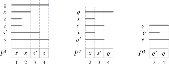
Figure C.2: Optimal plans of PlanM-Memoryless in steps $1$, $2$ and $3$.

Step $2$: The pending packets are $\varrho,x,s^{\prime},{\dot{x}},\varrho^{\prime}$ and the optimal plan is $P^{2}={\left\{x,s^{\prime},\varrho\right\}}$. Also, $\textsf{sub}^{2}(s^{\prime})=\varrho^{\prime}$, $\textsf{sub}^{2}(x)=x$, $\textsf{sub}^{2}(\varrho)$ is a packet of weight $0$, and

$$w_{s^{\prime}}+\phi{\,}w_{\varrho^{\prime}}\; =\;2+2\epsilon+\phi\cdot\phi^{-2}\;=\;(1+\phi)w_{x}+2\epsilon\;>\;w_{x}+\phi{\,}w_{x},$$

$$w_{s^{\prime}}+\phi{\,}w_{\varrho^{\prime}}\; >\;w_{\varrho}+\phi{\,}0,$$

so the algorithm will transmit $p=s^{\prime}$.

Step $3$: The pending packets are $\varrho^{\prime},\varrho,e$, the optimal plan is $P^{3}={\left\{\varrho^{\prime},\varrho\right\}}$, $\textsf{sub}^{3}(\varrho)=e$, $\textsf{sub}^{3}(\varrho^{\prime})=\varrho^{\prime}$, and

$$w_{\varrho}+\phi{\,}w_{e}\;=\;(1+\phi)w_{\varrho^{\prime}}+(\phi-1)\epsilon\;>\;w_{\varrho^{\prime}}+\phi{\,}w_{\varrho^{\prime}},$$

so the algorithm will transmit $p=\varrho$.

Step $4$: The only (non-zero weight) pending packet for the algorithm in this step is $e$, so this is the packet transmitted.

It remains to calculate the profits of PlanM-Memoryless and of OPT. As ${\epsilon}$ can be made arbitrarily small, in these calculations we assume that ${\epsilon}=0$. We also assume for simplicity that the three interleaved geometric sequences are backwards-infinite. Recall that $\sum_{i=0}^{\infty}\phi^{-2i}=\phi$.

For OPT, the profit in steps $...-2,-1,0$ from the three interleaved geoemtric sequences, is $\phi(w_{\varrho}+w_{x}+w_{z})=\phi(1+1+\phi)=3\phi+1$. Its profit in steps $1,\dots,4$ is $w_{{\dot{z}}}+w_{{\dot{x}}}+w_{s^{\prime}}+w_{s}=\phi+1+2+\phi^{2}=2\phi+4$. In total, $w({\textsf{OPT}})=5\phi+5$.

The profit of the algorithm in steps $...,-2,-,1,0$ is $\phi^{-2}$ times that of OPT, that is, $(3\phi+1)/\phi^{2}=\phi+\phi^{-1}$. In steps $1,\dots,4$, its profit is $w_{s}+w_{s^{\prime}}+w_{\varrho}+w_{e}=\phi^{2}+2+1+0=\phi+4$. Thus, $w({\textsf{ALG}})=\phi+\phi^{-1}+\phi+4=3\phi+3$, and thus the ratio equals $w({\textsf{OPT}})/w({\textsf{ALG}})=5/3>\phi$. (In fact, a slightly higher ratio can be achieved by having four interleaved geometric sequences, which would allow the optimal schedule to also include the packet corresponding to $\varrho^{\prime}$.)

Finally, we remark that even if we parameterize PlanM-Memoryless by $\alpha$ and select a packet $p$ maximizing $w_{p}+\alpha\cdot w(\textsf{sub}^{t}(p))$, we do not obtain a $\phi$-competitive algorithm. It would be interesting to know the competitive ratio of PlanM-Memoryless for the best choice of $\alpha$. The currently best memoryless deterministic algorithm is $1.893$-competitive [14].

Comparison to Algorithm PlanM. For comparison, consider what will our Algorithm PlanM do on this instance. The computation up to and including step 0 will be identical to that of PlanM-Memoryless. In step 1 the same packet $s$ will be transmitted, but the weight of its substitute packet $\varrho$ will be increased to $1$ in Line 4 of the algorithm. Similarly, in step 2 $s^{\prime}$ will be transmitted, but the weight of its substitute packet $\varrho^{\prime}$ will be increased to $1$. Then, in step 3 PlanM will transmit $\varrho^{\prime}$ (whose weight is now $1$) and in step 4 it will transmit $\varrho$. This will increase the profit of the algorithm by $w^{0}_{\varrho^{\prime}}=1/\phi^{2}$ (the original weight of $\varrho^{\prime}$), and its competitive ratio on this instance will be $\frac{5\phi+5}{3\phi+3+1/\phi^{2}}<\phi$.

C.2 Counterexample for Simpler Variants of PlanM

As explained in Appendix A, the value of ${\textsf{minwt}}^{t}(\tau)$ may decrease only if a packet $p$ from a non-initial segment of $P^{t}$ is transmitted. This is because in such a case $p$ is replaced in the optimum plan by a packet $\varrho$ with $w_{\varrho}<{\textsf{minwt}}^{t}(d_{\varrho})$. PlanM maintains the slot-monotonicity property by adjusting the weights and deadlines of some pending packets. First, it increases the weight of the substitute packet $\varrho$ to ${\textsf{minwt}}^{t}(d_{\varrho})$. The example in the previous section showed how this weight increase of $\varrho$ helps in reducing the overall ratio on some instances.

Second, if $\textsf{nextts}^{t}(d_{p})<\textsf{nextts}^{t}(d_{\varrho})$ (i.e., in an iterated leap step), then PlanM also makes an intricate shift of iteratively chosen packets $h_{1},\dots,h_{k}$. This shift is implemented by decreasing the deadlines and it prevents the algorithm from merging segments of $P^{t}$. In this section we address the question whether this shift process is necessary. To this end, we consider two simpler variants of PlanM that maintain the slot-monotonicity property as well, but do not perform an iterative shift of packets $h_{1},\dots,h_{k}$. Both variants only differ from PlanM in iterated leap steps, i.e., they use the same rule for choosing a packet to transmit and also increase the weight of $\varrho$ to ${\textsf{minwt}}^{t}(d_{\varrho})$ in each leap step.

In the first variant, called PlanM-Simpler and defined in Algorithm 3, instead of choosing packets $h_{1},\dots,h_{k}$, we identify the heaviest packet ${h^{\ast}}$ in the segment of $P^{t}$ containing $d^{t}_{\varrho}$, we decrease its deadline to $\textsf{nextts}^{t}(d_{p})$, and, if its weight is too small to preserve slot monotonicity, then we appropriately increase it. Recall that $\alpha=\textsf{nextts}^{t}(t)$ is the first tight slot of $P^{t}$.

Algorithm 3 Algorithm PlanM-Simpler ($t$)

1:transmit packet $p\in{{{P}}^{t}}$ that maximizes $w^{t}_{p}+\phi\cdot w^{t}(\textsf{sub}^{t}(p))$

2:if $d^{t}_{p}>\alpha$ then $\triangleright$ “leap step”

3:     $\varrho\,{\leftarrow}\,\textsf{sub}^{t}(p)$

4:     $w^{t+1}_{\varrho}\,{\leftarrow}\,{\textsf{minwt}}^{t}(d^{t}_{\varrho})$ $\triangleright$ increase $w_{\varrho}$

5:     $\eta\,{\leftarrow}\,\textsf{nextts}^{t}(d^{t}_{p})$ and $\gamma\,{\leftarrow}\,\textsf{nextts}^{t}(d^{t}_{\varrho})$

6:     if $\gamma>\eta$ then

7:         ${h^{\ast}}\,{\leftarrow}\,$ heaviest packet in $P^{t}(\textsf{prevts}^{t}(d^{t}_{\varrho}),\gamma]$

8:         $d^{t+1}_{{h^{\ast}}}\,{\leftarrow}\,\eta$ and $w^{t+1}_{{h^{\ast}}}\,{\leftarrow}\,\max\big{(}w^{t}_{{h^{\ast}}},{\textsf{minwt}}^{t}(\eta)\big{)}$      

The second variant is even simpler as we just decrease the deadline of $\varrho$ if it is after $\textsf{nextts}^{t}(d^{t}_{p})$ and increase $w_{\varrho}$ to match the minimum of ${\textsf{minwt}}()$ in its new segment. We call this algorithm PlanM-EvenSimpler and summarize it in Algorithm 4.

Algorithm 4 Algorithm PlanM-EvenSimpler ($t$)

1:transmit packet $p\in{{{P}}^{t}}$ that maximizes $w^{t}_{p}+\phi\cdot w^{t}(\textsf{sub}^{t}(p))$

2:if $d^{t}_{p}>\alpha$ then $\triangleright$ “leap step”

3:     $\varrho\,{\leftarrow}\,\textsf{sub}^{t}(p)$

4:     $d^{t+1}_{\varrho}\,{\leftarrow}\,\min\big{(}\,d^{t}_{\varrho},\textsf{nextts}^{t}(d^{t}_{p})\,\big{)}$

5:     $w^{t+1}_{\varrho}\,{\leftarrow}\,{\textsf{minwt}}^{t}(d^{t+1}_{\varrho})$ $\triangleright$ increase $w_{\varrho}$

Instance with ratio above $\phi$.

We now present a hard instance, for which the ratio of both algorithms exceeds $\phi$. The weights of some packets in this instance are parametrized by a parameter $\epsilon>0$, that can be made arbitrarily small.

Our instance is an extension of the lower-bound instance for PlanM-Memoryless described in Section C.1. In this instance we will use five (instead of just three) backwards-infinite interleaving sequences of packets whose weights increase geometrically by factor $\phi^{2}$. These packets will have span $6$. The principle is the same as in Section C.1: At each step $t$ the algorithm will have six packets $a_{0},a_{1},...,a_{5}$ pending, with each $a_{i}$ having its deadline at $t+i$. The weights will satisfy $w_{a_{0}}\leq w_{a_{i}}\leq\phi^{2}w_{a_{0}}$ for $i=2,3,4$ and $w_{a_{5}}=\phi^{2}w_{a_{0}}$. Thus, breaking the tie, the algorithm will transmit $a_{0}$ at each such step. This way, at each step the current ratio between the optimum profit and the algorithm’s profit will be $\phi^{2}$, although the algorithm will always have some remaining heavy packets pending that are not pending in the optimum schedule. At the end of the instance we release several new packets that will be transmitted by the algorithm instead of these older pending packets (which will expire).

Figure C.3 shows the complete instance. It also shows the schedules of PlanM-Simpler (also represented by striped yellow rectangles), of PlanM-EvenSimpler, and of an optimal solution (pink rectangles). Note that the schedules of PlanM-Simpler and PlanM-EvenSimpler are essentially the same, as the only difference is that slots of $h$ and $\varrho$ are swapped.

We now explain the behavior of PlanM-Simpler on instance in Figure C.3 (for PlanM-EvenSimpler, it is nearly the same). As explained earlier, the instance starts with five interleaved sequences of packets ${\left\{\varrho_{i}\right\}}_{i=1}^{\infty}$, ${\left\{x_{i}\right\}}_{i=1}^{\infty}$, ${\left\{h_{i}\right\}}_{i=1}^{\infty}$, ${\left\{r_{i}\right\}}_{i=1}^{\infty}$, and ${\left\{z_{i}\right\}}_{i=1}^{\infty}$, all of span $6$, with weights forming a geometric sequence with factor $\phi^{2}$. We think about these as being grouped into batches of $5$. Both algorithms PlanM-Simpler and PlanM-EvenSimpler will transmit tight packets in each step, while the adversary will always choose the heaviest packet to schedule. Later we have one more batch of five packets. These packets have different spans but their weights extend these geometric sequences, so we call them $\varrho=\varrho_{0}$, $x=x_{0}$, $h=h_{0}$, $r=r_{0}$ and $z=z_{0}$. For these packets the same basic principle applies, and in steps $-5,-4,-3,-2,-1$ the algorithm’s schedule will follow the same pattern. In step 0, for the same reason again, the tight packet $r$ will be transmitted.

packet $q$	initial weight $w_{q}$
$\varrho$	$1-\epsilon$
$\varrho_{i}$	$\phi^{-2i}w_{\varrho}$
$x$	$1$
$x_{i}$	$\phi^{-2i}w_{x}$
$h$	$1$
$h_{i}$	$\phi^{-2i}w_{h}$
$r$	$1+2\epsilon$
$r_{i}$	$\phi^{-2i}w_{r}$
$z$	$\phi$
$z_{i}$	$\phi^{-2i}w_{z}$
$s$	$\phi^{2}+2\epsilon$
$g$	$\phi^{2}$
$z^{\prime}$	$\phi-\epsilon$
$y$	$\phi-\epsilon$
$g^{\prime}$	$\phi^{2}-\epsilon$
$\varrho^{\prime}$	$1-\epsilon$

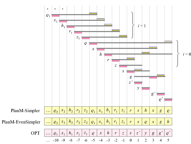
Figure C.3: An example for algorithms PlanM-Simpler and PlanM-EvenSimpler. The original packet weights are in the table on the left; packet spans are depicted in the figure, represented by a thick line segment. At the bottom, the figure shows the schedules of algorithms PlanM-Simpler and PlanM-EvenSimpler, as well as the optimum schedule. The schedules of PlanM-Simpler are also represented by unit-length thin rectangles (pink for the optimum and yellow and striped for PlanM-Simpler) attached to the line segments representing packet spans.

The crucial step is step 1. In this step PlanM-Simpler transmits packet $p=s$, since $s$ is the heaviest pending packet, $\varrho$ is the only substitute packet available, and $w_{s}+\phi w_{\varrho}>\phi^{2}w_{z}$, which holds for all $\epsilon>0$. PlanM-Simpler increases the weight of $\varrho$ to ${\textsf{minwt}}(5)=1$, decreases the deadline of packet $h$ to $2$, and increases its weight of $h$ to ${\textsf{minwt}}(2)=\phi$. This is illustrated in Figure C.4, that shows the optimal plans of PlanM-Simpler in step 1 and step 2. (PlanM-EvenSimpler also transmits $p=s$, decreases the deadline of $\varrho$ to $2$, and increases its weight to $\phi$.)

packet	weight $w^{1}$
$\varrho$	$1-\epsilon$
$x$	$1$
$h$	$1$
$z$	$\phi$
$s$	$\phi^{2}+2\epsilon$
$g$	$\phi^{2}$
$z^{\prime}$	$\phi-\epsilon$

packet	weight $w^{2}$
$\varrho$	$1$
$x$	$1$
$h$	$\phi$
$g$	$\phi^{2}$
$y$	$\phi-\epsilon$

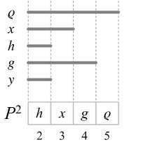
Figure C.4: Optimal plans of PlanM-Simpler in steps $1$ and $2$. The tables show packet weights. Note that the weight of $\varrho$ changed, and for $h$ both the deadline and weight changed.

After step 1, there are no leap steps in the remaining four steps as there won’t be any non-expiring packet outside the optimal plan (that could serve as a non-zero weight substitute packet) and at each step the weights of pending packets are within a factor of $\phi^{2}$. (Note that packet $y$ will not appear in the plan in step 2, even though it is heavier than the original weight of $h$.)

Next, we calculate the profits. Since $\epsilon$ can be made arbitrarily small, in the calculations we can assume that $\epsilon=0$. For the optimal schedule, adding up the weights of the five interleaved packet sequences, up to step -1, their total weight is $\phi(w_{\varrho}+w_{x}+w_{h}+w_{r}+w_{z})=5\phi+1$. (Recall that $\sum_{i=0}^{\infty}\phi^{-2i}=\phi$.) The optimal profit in steps $0,1,...,5$ is $w_{s}+w_{z^{\prime}}+w_{y}+w_{g}+w_{g^{\prime}}+w_{\varrho^{\prime}}=\phi^{2}+\phi+\phi+\phi^{2}+\phi^{2}+1=5\phi+4$. Thus $w({\textsf{OPT}})=10\phi+5$.

The profit of either algorithm before step $0$ (i.e., from the five interleaved sequences) is smaller by factor of $\phi^{2}$ than the corresponding profit in the optimum schedule, so it equals $(5\phi+1)/\phi^{2}=4\phi-3$. The algorithm’s profit in steps $0,1,...,5$ is $w_{r}+w_{s}+w_{h}+w_{x}+w_{g}+w_{\varrho}=1+\phi^{2}+1+1+\phi^{2}+1=2\phi+6$. (Here, of course, we take the original weights into account). Thus its total profit is $w({\textsf{ALG}})=6\phi+3$, giving us ratio $w({\textsf{OPT}})/w({\textsf{ALG}})=5/3\approx 1.666$.

What goes wrong in the analysis.

We explain where the analysis in the paper fails for Algorithm PlanM-Simpler (the reason is basically the same for PlanM-EvenSimpler). Consider step 1, and assume that $\epsilon=0$. In this step, using the profit of $\phi\cdot w_{s}=\phi^{3}$, the algorithm needs to “pay” for all of the following: (i) the adversary profit from $z^{\prime}$, equal to $\phi$, (ii) removing $z$ and $s$ from ${{\mathcal{B}}}$, which costs $1+\phi$, (iii) increasing the weight of $\varrho$, which is negligible, and (iv) increasing the weight of $h$, which costs $\phi^{-1}$, as the potential increases as well. The total cost thus sums to $\phi^{3}+\phi^{-1}$; it is no coincidence that the excess of $\phi^{-1}$ over the profit equals $w({\textsf{OPT}})-\phi\cdot w({\textsf{ALG}})$, since all other steps are essentially tight (in terms of calculations in the analysis).

Comparison to Algorithm PlanM. For comparison, consider what our Algorithm PlanM does on this instance. The computation up to and including step 0 remains identical to that of PlanM-Simpler. We focus on step 1. In step 1 the same packet $s$ gets transmitted, and the weight of $\varrho$ is also increased to $1$. However, PlanM further performs its iterative shift, with $k=2$, $h_{1}=g$, and $h_{2}=h$. Figure C.5 shows the effect of this change on the plan in step 2, in which PlanM transmits $g$, unlike PlanM-Simpler which transmits $h$ in this step.

packet	weight $w^{1}$
$\varrho$	$1-\epsilon$
$x$	$1$
$h$	$1$
$z$	$\phi$
$s$	$\phi^{2}+2\epsilon$
$g$	$\phi^{2}$
$z^{\prime}$	$\phi-\epsilon$

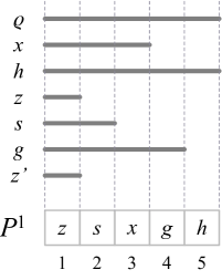
packet	weight $w^{2}$
$\varrho$	$1$
$x$	$1$
$h$	$1$
$g$	$\phi^{2}$
$y$	$\phi-\epsilon$

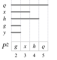
Figure C.5: Optimal plans of Algorithm PlanM in steps $1$ and $2$. The tables show packet weights before the corresponding steps. Note the the weight of packet $\varrho$ was changed, and the deadlines of packets $g$ and $h$ were reduced.

References

- [1] Gagan Aggarwal, Gagan Goel, Chinmay Karande, and Aranyak Mehta. Online vertex-weighted bipartite matching and single-bid budgeted allocations. In Proc. of the 22nd Annual ACM-SIAM Symposium on Discrete Algorithms (SODA ’11), pages 1253–1264, 2011.
- [2] William A. Aiello, Yishay Mansour, S. Rajagopolan, and Adi Rosén. Competitive queue policies for differentiated services. J. Algorithms, 55(2):113–141, 2005.
- [3] Nir Andelman, Yishay Mansour, and An Zhu. Competitive queueing policies for QoS switches. In Proc. of the 14th Annual ACM-SIAM Symposium on Discrete Algorithms (SODA ’03), pages 761–770, 2003.
- [4] Yair Bartal, Francis Y. L. Chin, Marek Chrobak, Stanley P. Y. Fung, Wojciech Jawor, Ron Lavi, Jiří Sgall, and Tomáš Tichý. Online competitive algorithms for maximizing weighted throughput of unit jobs. In Proc. of the 21st Symposium on Theoretical Aspects of Computer Science (STACS ’04), volume 2996 of LNCS, pages 187–198. Springer Berlin Heidelberg, 2004.
- [5] Marcin Bienkowski, Marek Chrobak, Christoph Dürr, Mathilde Hurand, Artur Jeż, Łukasz Jeż, and Grzegorz Stachowiak. Collecting weighted items from a dynamic queue. Algorithmica, 65(1):60–94, 2013.
- [6] Marcin Bienkowski, Marek Chrobak, Christoph Dürr, Mathilde Hurand, Artur Jeż, Łukasz Jeż, and Grzegorz Stachowiak. A -competitive algorithm for collecting items with increasing weights from a dynamic queue. Theoretical Computer Science, 475:92 – 102, 2013.
- [7] Marcin Bienkowski, Marek Chrobak, and Łukasz Jeż. Randomized competitive algorithms for online buffer management in the adaptive adversary model. Theoretical Computer Science, 412(39):5121–5131, 2011.
- [8] Martin Böhm, Marek Chrobak, Łukasz Jeż, Fei Li, Jiří Sgall, and Pavel Veselý. Online packet scheduling with bounded delay and lookahead. Theoretical Computer Science, 776:95 – 113, 2019.
- [9] Francis Y. L. Chin, Marek Chrobak, Stanley P. Y. Fung, Wojciech Jawor, Jiří Sgall, and Tomáš Tichý. Online competitive algorithms for maximizing weighted throughput of unit jobs. J. of Discrete Algorithms, 4(2):255–276, 2006.
- [10] Francis Y. L. Chin and Stanley P. Y. Fung. Online scheduling with partial job values: Does timesharing or randomization help? Algorithmica, 37(3):149–164, 2003.
- [11] Marek Chrobak, Wojciech Jawor, Jiří Sgall, and Tomáš Tichý. Improved online algorithms for buffer management in QoS switches. In Proc. of the 12th Annual European Symposium on Algorithms (ESA ’04), volume 3221 of LNCS, pages 204–215, 2004.
- [12] Marek Chrobak, Wojciech Jawor, Jiří Sgall, and Tomáš Tichý. Improved online algorithms for buffer management in QoS switches. ACM Trans. Algorithms, 3(4), 2007.
- [13] Nikhil R. Devanur, Kamal Jain, and Robert D. Kleinberg. Randomized primal-dual analysis of RANKING for online bipartite matching. In Proc. of the 24th Annual ACM-SIAM Symposium on Discrete Algorithms (SODA ’13), pages 101–107, 2013.
- [14] Matthias Englert and Matthias Westermann. Considering suppressed packets improves buffer management in quality of service switches. SIAM Journal on Computing, 41(5):1166–1192, 2012.
- [15] Michael H. Goldwasser. A survey of buffer management policies for packet switches. SIGACT News, 41(1):100–128, 2010.
- [16] Bruce Hajek. On the competitiveness of on-line scheduling of unit-length packets with hard deadlines in slotted time. In Proc. of the 35th Conference on Information Sciences and Systems, pages 434–438, 2001.
- [17] Łukasz Jeż, Fei Li, Jay Sethuraman, and Clifford Stein. Online scheduling of packets with agreeable deadlines. ACM Trans. Algorithms, 9(1):5:1–5:11, 2012.
- [18] Alexander Kesselman, Zvi Lotker, Yishay Mansour, Boaz Patt-Shamir, Baruch Schieber, and Maxim Sviridenko. Buffer overflow management in QoS switches. SIAM Journal on Computing, 33(3):563–583, 2004.
- [19] Fei Li, Jay Sethuraman, and Clifford Stein. An optimal online algorithm for packet scheduling with agreeable deadlines. In Proc. of the 16th Annual ACM-SIAM Symposium on Discrete Algorithms (SODA ’05), pages 801–802, 2005.
- [20] Fei Li, Jay Sethuraman, and Clifford Stein. Better online buffer management. In Proc. of the 18th Annual ACM-SIAM Symposium on Discrete Algorithms (SODA ’07), pages 199–208, 2007.
- [21] Pavel Veselý. Packet scheduling: Plans, monotonicity, and the golden ratio. SIGACT News, 52(2):72–84, June 2021.
- [22] Pavel Veselý, Marek Chrobak, Lukasz Jez, and Jirí Sgall. A -competitive algorithm for scheduling packets with deadlines. In Timothy M. Chan, editor, Proceedings of the Thirtieth Annual ACM-SIAM Symposium on Discrete Algorithms, SODA 2019, San Diego, California, USA, January 6-9, 2019, pages 123–142. SIAM, 2019. doi:10.1137/1.9781611975482.9.
- [23] Pavel Veselý, Marek Chrobak, Lukasz Jez, and Jirí Sgall. A \(\boldsymbol{\phi }\) -competitive algorithm for scheduling packets with deadlines. SIAM J. Comput., 51(5):1626–1691, 2022. doi:10.1137/21m1469753.
- [24] An Zhu. Analysis of queueing policies in QoS switches. J. Algorithms, 53(2):137–168, 2004.
- [25] Łukasz Jeż. A universal randomized packet scheduling algorithm. Algorithmica, 67(4):498–515, 2013.