Measurement and Quantum Dynamics in the Minimal Modal Interpretation of Quantum Theory

Abstract

Any realist interpretation of quantum theory must grapple with the measurement problem and the status of state-vector collapse. In a no-collapse approach, measurement is typically modeled as a dynamical process involving decoherence. We describe how the minimal modal interpretation closes a gap in this dynamical description, leading to a complete and consistent resolution to the measurement problem and an effective form of state collapse. Our interpretation also provides insight into the indivisible nature of measurement—the fact that you can’t stop a measurement part-way through and uncover the underlying ‘ontic’ dynamics of the system in question. Having discussed the hidden dynamics of a system’s ontic state during measurement, we turn to more general forms of open-system dynamics and explore the extent to which the details of the underlying ontic behavior of a system can be described. We construct a space of ontic trajectories and describe obstructions to defining a probability measure on this space.

1 Introduction

Consider the axioms governing the dynamics of quantum systems as set out by Dirac and von Neumann [1, 2]:

1. Unitary Evolution: When a quantum system is closed, its state vector evolves according to the Schrödinger equation.

2. Collapse: When a measurement is performed, the state vector collapses into one of the measurement’s mutually exclusive outcomes.

The reference to measurements within these axioms is deeply problematic. One could posit that measurement is somehow fundamental, but then how does one rigorously determine in a practical, physical scenario under what precise circumstances one should declare that a measurement has taken place? Is there a sharp way to define which kinds of systems are capable of carrying out measurements and which are not? And if measurements are not fundamental, but are instead processes carried out on quantum states by measurement devices that register their results in terms of quantum states of their own, how does one avoid charges of circular reasoning that stem from the assertion that quantum states are nothing more than collections of probabilities for measurement outcomes?

Any interpretation of quantum theory that claims to refrain from making any metaphysical commitments about the state of existence of physical systems immediately runs into the problem of requiring the existence of systems that can carry out measurements in line with the standard axioms. On the other had, any realist interpretation of quantum theory that involves fundamental collapse must still grapple with these issues.

An alternative is to formulate a no-collapse realist interpretation of quantum theory. One primary task of such an interpretation is to explain the appearance of collapse. The de Broglie-Bohm pilot-wave interpretation [4, 5] and the Everett-DeWitt many-worlds interpretation [6, 7] are both prominent examples of the no-collapse approach. The traditional pilot-wave interpretation asserts that particles have simultaneously well-defined positions and momenta at all times—these quantities are elements of the universe’s ontology, meaning its fundamental state of being. The wave function plays the role of a ‘pilot wave’: a field defined on the system’s configuration space that ensures that the particles’ behaviors are effectively captured by the usual rules of quantum theory. For example, the pilot wave ensures that the measured values of the particles’ momenta exhibit the statistical spread required by the uncertainty principle. In this situation, as Bohm himself originally explained, decoherence ensures that collapse emerges purely phenomenologically from treating both the system to be measured and the measurement device according to the rules of quantum theory.

The many-worlds interpretation, like the pilot-wave interpretation, postulates that the entire universe behaves as a closed quantum system with a ‘universal state vector.’ In the many-worlds interpretation, the universal state vector is the key element of the ontology. In this picture, collapse is only apparent because we are subsystems that are part of the overall state of the universe, and when we entangle with the outcome states of a measurement apparatus, the different outcomes and our perceptions of those outcomes lie on separate ‘branches’ of the universal state vector. These branches, roughly speaking, are the interpretation’s ‘worlds.’

Both approaches suffer from severe shortcomings, many of which have been examined in the literature [8, 9]. In this paper, we focus on the measurement problem through the lens of the minimal modal interpretation. Unlike the de Broglie-Bohm interpretation, which defines a system’s ontology as always consisting of hidden positions and momenta that are nowhere to be found within the standard quantum formalism, our interpretation embraces minimalism by adhering more closely to the ingredients of textbook quantum theory, allowing the ontology of a system to evolve dynamically so that the fundamental properties posessed by the system may change with time. This minimalist approach helps ensure that our interpretation extends to all types of quantum systems, both relativistic and non-relativistic, with no need for modification. Furthermore, the minimal modal interpretation is a ‘single-world’ interpretation in the sense of asserting definite outcomes for measurements and thereby dodging several of the problems that many-worlds-type approaches run into. We describe how our interpretation avoids these problems in [11].

In Section 2, we lay out the axioms that define the minimal modal interpretation. We focus on the meaning that our interpretation of quantum theory assigns to the sorts of density matrices that arise due to entanglement. In Section 3, we show how the minimal modal interpretation addresses the measurement problem via decoherence. Section 4 explores the extent to which the evolution of the actual state of a quantum system can be made explicit during processes such as measurements, as well as the role of non-probabilistic (or ‘Knightian’ [12, 13]) uncertainty in hiding the trajectory of this underlying state. We conclude in Section 5 with a summary and some ideas for future directions.

2 The Minimal Modal Interpretation

2.1 Axioms

Historically, modal interpretations have represented a way to talk about quantum states of systems in terms of possible or actual ontic states, where ‘ontic’ denotes an ontological or existential feature of the universe rather than an aspect of observation. The minimal modal interpretation identifies a system’s density-matrix eigenstates with the system’s set of possible ontic states at any given moment. The corresponding eigenvalues encode probabilistic uncertainty about which of these ontic states is actually occupied by the system. The usual quantum laws governing the time evolution of the density matrix are supplemented with a set of quantum conditional probabilities that govern the dynamics of the system’s possible ontic states over time.

More precisely, the interpretation is defined by the following axioms.

1. Ontic States: A given quantum system at any particular instant of time $t$ has a mutually exclusive set of possible ontic states $\mathopen{}\mathclose{{}\left\{\Psi_{i}(t)}\right\}$ that collectively form the system’s dynamical configuration space. The system’s actual ontic state is one of these possibilities. The possible ontic states correspond to a set of mutually orthogonal, unit-norm state vectors in the system’s Hilbert space $\mathcal{H}$:

   $$\Psi_{i}(t) \iff|\Psi_{i}(t)\rangle\in\mathcal{H}\ \textrm{(defined up to an overall phase),}$$ (1)

   $$\Psi_{i}(t),\Psi_{j}(t) \iff\mathopen{}\mathclose{{}\left\langle\Psi_{i}(t)|\Psi_{j}(t)}\right\rangle=\delta_{ij}\ \textrm{(mutual exclusivity)}.$$ (2)

2. Objective Epistemic States: Objective epistemic states are probability distributions over the system’s set of possible ontic states:

   $$\mathopen{}\mathclose{{}\left\{\mathopen{}\mathclose{{}\left(p_{i}(t),\Psi_{i}(t)}\right)}\right\}_{i},\ \ \ p_{i}(t)\in\mathopen{}\mathclose{{}\left[0,1}\right].$$ (3)

   The probabilities here are interpreted as arising from objective uncertainty as to the true ontic state of the system. Objective epistemic states can be encoded as density matrices, meaning positive-semidefinite, unit-trace operators:

   $$\mathopen{}\mathclose{{}\left\{\mathopen{}\mathclose{{}\left(p_{i}(t),\Psi_{i}(t)}\right)}\right\}_{i}\iff\hat{\rho}\mathopen{}\mathclose{{}\left(t}\right)=\sum_{i}p_{i}(t)\mathopen{}\mathclose{{}\left|\Psi_{i}(t)\mathopen{}\mathclose{{}\left\rangle}\right\langle\Psi_{i}(t)}\right|=\sum_{i}p_{i}(t)\hat{P}\mathopen{}\mathclose{{}\left(i;t}\right).$$ (4)

   Here $\hat{P}\mathopen{}\mathclose{{}\left(i;t}\right)=\mathopen{}\mathclose{{}\left|\Psi_{i}(t)\mathopen{}\mathclose{{}\left\rangle}\right\langle\Psi_{i}(t)}\right|$ is the eigenprojector corresponding to the density-matrix eigenstate $|\Psi_{i}(t)\rangle$ at time $t$. Note, however, that not all density matrices correspond to objective epistemic states, as we explain in Section 2.2.

3. Subsystems and System-Centric Ontology:

   1. Let $W=Q+E$ denote a parent system consisting of a subsystem $Q$ and its larger environment $E$, and let $\hat{\rho}_{W}$ denote the density matrix representing the objective epistemic state of $W$. The objective epistemic state of $Q$ corresponds to the partial trace

      $$\hat{\rho}_{Q}(t)\equiv\textrm{Tr}_{E}\mathopen{}\mathclose{{}\left[\hat{\rho}_{W}(t)}\right].$$ (5)

      The previous axioms then define the ontic and objective epistemic states of $Q$.

   2. The ontology of a given system is defined solely via the eigenvectors of that system’s own (reduced) density matrix. The density-matrix eigenvectors of other systems are irrelevant. We call this notion system-centric ontology.

4. Quantum Conditional Probabilities: Let $W=Q_{1}+Q_{2}$ be a parent system that is subdivided into two mutually disjoint subsystems $Q_{1}$ and $Q_{2}$. Let $\hat{\rho}_{W}\mathopen{}\mathclose{{}\left(t}\right)$ be the density matrix describing the parent system’s objective epistemic state at time $t$. When the time evolution of this density matrix from one time $t$ to another time $t^{\prime}$ is well-approximated by a linear completely positive and trace-preserving (CPTP) mapping,

   $$\mathcal{E}_{W}^{t^{\prime}\leftarrow t}:\hat{\rho}_{W}\mathopen{}\mathclose{{}\left(t}\right)\mapsto\mathcal{E}_{W}^{t^{\prime}\leftarrow t}\mathopen{}\mathclose{{}\left\{\hat{\rho}_{W}\mathopen{}\mathclose{{}\left(t}\right)}\right\},$$ (6)

   which generalizes the notion of unitary time evolution, we can define quantum conditional probabilities in the following way:

   $$p_{Q_{1},Q_{2}|W}\mathopen{}\mathclose{{}\left(i_{1},i_{2};t^{\prime}|w;t}\right)\equiv\textrm{Tr}_{W}\mathopen{}\mathclose{{}\left[\mathopen{}\mathclose{{}\left(\hat{P}_{Q_{1}}\mathopen{}\mathclose{{}\left(i_{1};t^{\prime}}\right)\otimes\hat{P}_{Q_{2}}\mathopen{}\mathclose{{}\left(i_{2};t^{\prime}}\right)}\right)\mathcal{E}_{W}^{t^{\prime}\leftarrow t}\mathopen{}\mathclose{{}\left\{\hat{P}_{W}\mathopen{}\mathclose{{}\left(w;t}\right)}\right\}}\right].$$ (7)

   This formula gives the joint conditional probability for finding the subsystems $Q_{1},Q_{2}$ in their respective ontic states $\Psi_{i_{1}},\Psi_{i_{2}}$ at time $t^{\prime}$ given that the parent system $W$ was in the ontic state $\Psi_{w}$ at time $t$.

In Appendix A, we motivate the definition in (7) and explain how it generalizes to joint conditional probabilities for any number of mutually disjoint subsystems. The conditional probabilities of Axiom 4 are only sharply defined to the extent that a system’s evolution during a particular time interval $t\to t^{\prime}$ is well-approximated by a linear CPTP mapping $\mathcal{E}_{W}^{t^{\prime}\leftarrow t}$. When these conditional probabilities are not sharply defined, the system continues to have an actual ontic state, but the uncertainty surrounding the time evolution of that state is non-probabilistic. We explore some of these issues in more depth in Section 4.6.

In our analysis of the measurement process, we make use of the special case in which $Q_{1}=W$ is the entire system and $Q_{2}$ is trivial. We have

$$p\mathopen{}\mathclose{{}\left(w^{\prime};t^{\prime}|w;t}\right) =\textrm{Tr}\mathopen{}\mathclose{{}\left[\hat{P}\mathopen{}\mathclose{{}\left(w^{\prime};t^{\prime}}\right)\mathcal{E}^{t^{\prime}\leftarrow t}\mathopen{}\mathclose{{}\left\{\hat{P}\mathopen{}\mathclose{{}\left(w;t}\right)}\right\}}\right],$$ (8)

where we have dropped system labels because now only one system is being considered. The conditional probabilities (8) describe the stochastic result of the time evolution of the system’s ontic state during a process that is approximated by linear CPTP dynamics. Exact unitary evolution is a particular, idealized case in which the system in question is completely isolated—a situation that is impossible to achieve in the real world.

One must resist the temptation to identify the smooth evolution of density-matrix eigenprojectors under a smooth, linear CPTP map with the trajectory of the system’s actual ontic state. This trajectory is generically hidden due to entanglement, as discussed in Section 4.

2.2 The Interpretation of Mixed States

Consider a closed quantum system that is fundamentally described by a state vector $|\Psi_{1}\rangle$ in a two-dimensional Hilbert space. Suppose, however, that you do not know with certainty that $|\Psi_{1}\rangle$ is the system’s state vector. Instead, letting $|\Psi_{2}\rangle$ denote the orthogonal state vector, unique up to overall phase, you can capture your ignorance by introducing a probability distribution $\mathopen{}\mathclose{{}\left\{p_{1},p_{2}}\right\}$ over the pair of mutually orthogonal state vectors $\mathopen{}\mathclose{{}\left\{|\Psi_{1}\rangle,|\Psi_{2}\rangle}\right\}$. The density matrix

$$\hat{\rho}=\sum_{i}p_{i}\mathopen{}\mathclose{{}\left|\Psi_{i}\mathopen{}\mathclose{{}\left\rangle}\right\langle\Psi_{i}}\right|=p_{1}\mathopen{}\mathclose{{}\left|\Psi_{1}\mathopen{}\mathclose{{}\left\rangle}\right\langle\Psi_{1}}\right|+p_{2}\mathopen{}\mathclose{{}\left|\Psi_{2}\mathopen{}\mathclose{{}\left\rangle}\right\langle\Psi_{2}}\right|$$ (9)

then represents an example of what’s called a proper mixture or a properly mixed state. The interpretation of this density matrix as encoding subjective ignorance regarding the system’s true state is completely standard and widely accepted.

By contrast, consider a parent system $W=A+B$, with $A$ and $B$ disjoint subsystems. Suppose that the parent system is in the pure state

$$c_{1}|\Psi_{A,1},\Psi_{B,1}\rangle+c_{2}|\Psi_{A,2},\Psi_{B,2}\rangle,$$

where $\mathopen{}\mathclose{{}\left|c_{1}}\right|^{2}+\mathopen{}\mathclose{{}\left|c_{2}}\right|^{2}=1$ and where the sets $\mathopen{}\mathclose{{}\left\{|\Psi_{A,\alpha}\rangle}\right\}_{\alpha}$ and $\mathopen{}\mathclose{{}\left\{|\Psi_{B,\beta}\rangle}\right\}_{\beta}$ consist of mutually orthogonal vectors in the respective Hilbert spaces of the subsystems $A$ and $B$. We also employ the standard notational convention

$$|\Psi_{A,\alpha},\Psi_{B,\beta}\rangle\equiv|\Psi_{A,\alpha}\rangle\otimes|\Psi_{B,\beta}\rangle.$$

Consider the reduced density matrix of subsystem $A$:

$$\hat{\rho}_{A}\equiv\textrm{Tr}_{B}\mathopen{}\mathclose{{}\left[\hat{\rho}}\right]=\mathopen{}\mathclose{{}\left|c_{1}}\right|^{2}\mathopen{}\mathclose{{}\left|\Psi_{A,1}\mathopen{}\mathclose{{}\left\rangle}\right\langle\Psi_{A,1}}\right|+\mathopen{}\mathclose{{}\left|c_{2}}\right|^{2}\mathopen{}\mathclose{{}\left|\Psi_{A,2}\mathopen{}\mathclose{{}\left\rangle}\right\langle\Psi_{A,2}}\right|.$$ (10)

This density matrix represents an example of an improper mixture. This density matrix (10) is identical in form to the density matrix of a proper mixture (9), but it arises in a very different context and, crucially, the standard axioms of quantum theory leave its interpretation unclear. The minimal modal interpretation fills in this gap by identifying the reduced density-matrix eigenstates, $|\Psi_{A,1}\rangle$ and $|\Psi_{A,2}\rangle$ with the mutually exclusive possible ontic states that the subsystem $A$ may occupy. Axiom 1 requires that $A$ in fact occupies one of these two possibilities. Axiom 2 asserts that the eigenvalues of this density matrix represent probabilities that describe fundamental probabilistic uncertainty.

The meaning that we assign to improper mixtures is quite natural: We interpret them as capturing probabilistic uncertainty about the state of the system in the same manner as do proper mixtures. The distinction between proper and improper mixtures lies in the origin of the uncertainty they encode. Proper mixtures involve subjective uncertainty—different observers may write down different density matrices depending on the information they have about the state of the system. By contrast, improper mixtures involve objective uncertainty—an irreducible level of uncertainty that is unique to quantum systems. Objective uncertainty arises due to entanglement between the system and its environment, and serves to mask the actual ontic state of the system.

3 The Measurement Problem

3.1 Conceptual Overview

Suppose that a system of interest—called here the subject system—is initially isolated and described by a given pure state. Measuring the system opens it up to the environment, resulting in entanglement between the system, the measurement device, and the overall environment. If the subject system began in a quantum superposition of states that can be experimentally distinguished by the measurement device, then the entanglement process leads to an effective loss of coherence at the level of the subject system, a process known as decoherence.

But the measurement problem doesn’t end with decoherence—because decoherence yields an improper mixture. There is a gap in going from this improperly mixed state to a proper mixture that would immediately lend itself to describing subjective uncertainty over a unique measurement outcome. Put a bit differently, if measurements induce entanglement between a subject system and a measurement device or the larger environment, why do we see a definite outcome? Decoherence alone cannot answer this question. In the absence of an explicit collapse postulate, this issue can only be resolved by going beyond the other traditional axioms of quantum theory.

The axioms of the minimal modal interpretation close this gap by identifying each system’s possible ontic states with the eigenstates of its objective density matrix. Decoherence forces the subject system’s possible ontic states to converge rapidly to the possible outcome states of the given measurement, differing only by exponentially small corrections arising from the residual coherence terms. The measurement device’s density matrix undergoes an analogous rapid convergence to corresponding possible outcome states. Although neither the subject system’s density matrix nor the measurement device’s density matrix are exactly diagonal in the expected basis, they can be made diagonal by exponentially small redefinitions of the measurement-outcome states. Furthermore, the actual ontic state of the subject system is axiomatically taken to be one of these ontic possibilities, and similarly for the measurement device, meaning that the overall measurement results in a definite outcome.

One concern that has been raised historically about modal interpretations surrounds the status of degeneracies in density matrices—that is, the case in which multiple eigenprojectors belonging to a single density matrix share precisely the same eigenvalue [8, 10]. In this scenario, a density matrix does not single out a unique set of orthonormal eigenstates, leading to ambiguities in the presumed ontology for the corresponding quantum system.

However, as explained in greater detail in [11], true degeneracies are impossible to realize in practice, as they correspond to measure-zero arrangements requiring infinite fine-tuning. What represents a more serious potential issue is the case of near-degeneracies that can arise during the decoherence process, as these near-degeneracies can ostensibly result in instabilities in the ontic states of macroscopic systems, such as measurement devices and the larger environment. The minimal modal interpretation’s fourth axiom—defining quantum conditional probabilities—ameliorates this issue. As long as the evolution of the systems in question is linear CPTP to a good approximation, the conditional probabilities smooth out the evolution of the ontic states, thereby avoiding undesirable ontic instabilities [11].

3.2 Measurements and Decoherence

Consider an initially isolated subject system $S$ and a system observable with orthonormal eigenbasis $\mathopen{}\mathclose{{}\left\{|m\rangle}\right\}_{m}$. A macroscopic measurement apparatus $A$ is initially prepared in a “blank” pure state $|A\mathopen{}\mathclose{{}\left(``\emptyset"}\right)\rangle$. The larger environment $E$ is initially in the pure state $|E\mathopen{}\mathclose{{}\left(``\emptyset"}\right)\rangle$, registering the apparatus’s blank state. We assume that the evolution of the total system is linear CPTP (if not unitary) and can be modeled as consisting largely of two steps.

1. If the subject system is in a pure state corresponding precisely to one of the measurement outcomes $|m\rangle$, then the apparatus transitions to a new pure state $|A\mathopen{}\mathclose{{}\left(``m"}\right)\rangle$ that registers the state of the subject system:

   $$|m\rangle|A\mathopen{}\mathclose{{}\left(``\emptyset"}\right)\rangle|E\mathopen{}\mathclose{{}\left(``\emptyset"}\right)\rangle\stackrel{{\scriptstyle\textrm{step }1}}{{\mapsto}}|m\rangle|A\mathopen{}\mathclose{{}\left(``m"}\right)\rangle|E\mathopen{}\mathclose{{}\left(``\emptyset"}\right)\rangle.$$ (11)

2. The environment then transitions to a pure state $|E\mathopen{}\mathclose{{}\left(``m"}\right)\rangle$ that observably registers in some way the change in the apparatus’s state—for example, through the transmission of outgoing thermal radiation:

   $$|m\rangle|A\mathopen{}\mathclose{{}\left(``m"}\right)\rangle|E\mathopen{}\mathclose{{}\left(``\emptyset"}\right)\rangle\stackrel{{\scriptstyle\textrm{step }2}}{{\mapsto}}|m\rangle|A\mathopen{}\mathclose{{}\left(``m"}\right)\rangle|E\mathopen{}\mathclose{{}\left(``m"}\right)\rangle.$$ (12)

Generalizing, suppose now that $|\Psi\rangle$ is the initial pure state of the subject system. Expanding it in terms of the measurement-outcome states,

$$|\Psi\rangle=\sum_{m}\Psi_{m}|m\rangle,$$ (13)

the assumed linearity of the dynamics then dictates that the foregoing two-step sequence applies to each individual term in the superposition:

$$|\Psi\rangle|A\mathopen{}\mathclose{{}\left(``\emptyset"}\right)\rangle|E\mathopen{}\mathclose{{}\left(``\emptyset"}\right)\rangle =\mathopen{}\mathclose{{}\left(\sum_{m}\Psi_{m}|m\rangle}\right)|A\mathopen{}\mathclose{{}\left(``\emptyset"}\right)\rangle|E\mathopen{}\mathclose{{}\left(``\emptyset"}\right)\rangle$$

$$\stackrel{{\scriptstyle\textrm{step }1}}{{\mapsto}}\mathopen{}\mathclose{{}\left(\sum_{m}\Psi_{m}|m\rangle|A\mathopen{}\mathclose{{}\left(``m"}\right)\rangle}\right)|E\mathopen{}\mathclose{{}\left(``\emptyset"}\right)\rangle$$ (14)

$$\stackrel{{\scriptstyle\textrm{step }2}}{{\mapsto}}\sum_{m}\Psi_{m}|m\rangle|A\mathopen{}\mathclose{{}\left(``m"}\right)\rangle|E\mathopen{}\mathclose{{}\left(``m"}\right)\rangle.$$ (15)

After the measurement, the reduced density matrix of the subject system takes the form

$$\hat{\rho}_{S}\mathopen{}\mathclose{{}\left(\Delta t}\right) =\sum_{\mathclap{m_{1},m_{2}}}\Psi_{m_{1}}\Psi_{m_{2}}^{*}\mathopen{}\mathclose{{}\left|m_{1}\mathopen{}\mathclose{{}\left\rangle}\right\langle m_{2}}\right|\mathopen{}\mathclose{{}\left\langle A\mathopen{}\mathclose{{}\left(``m_{2}"}\right)|A\mathopen{}\mathclose{{}\left(``m_{1}"}\right)}\right\rangle\mathopen{}\mathclose{{}\left\langle E\mathopen{}\mathclose{{}\left(``m_{2}"}\right)|E\mathopen{}\mathclose{{}\left(``m_{1}"}\right)}\right\rangle$$

$$=\sum_{m}\mathopen{}\mathclose{{}\left|\Psi_{m}}\right|^{2}\mathopen{}\mathclose{{}\left|m\mathopen{}\mathclose{{}\left\rangle}\right\langle m}\right|+\sum_{\mathclap{\begin{subarray}{c}m_{1},m_{2}\\ m_{1}\neq m_{2}\end{subarray}}}\Psi_{m_{1}}\Psi_{m_{2}}^{*}\mathopen{}\mathclose{{}\left|m_{1}\mathopen{}\mathclose{{}\left\rangle}\right\langle m_{2}}\right|\mathopen{}\mathclose{{}\left\langle A\mathopen{}\mathclose{{}\left(``m_{2}"}\right)|A\mathopen{}\mathclose{{}\left(``m_{1}"}\right)}\right\rangle\mathopen{}\mathclose{{}\left\langle E\mathopen{}\mathclose{{}\left(``m_{2}"}\right)|E\mathopen{}\mathclose{{}\left(``m_{1}"}\right)}\right\rangle,$$ (16)

where $\Delta t$ is the time duration of the measurement. The quantities $\mathopen{}\mathclose{{}\left\langle A\mathopen{}\mathclose{{}\left(``m_{2}"}\right)|A\mathopen{}\mathclose{{}\left(``m_{1}"}\right)}\right\rangle$ and $\mathopen{}\mathclose{{}\left\langle E\mathopen{}\mathclose{{}\left(``m_{2}"}\right)|E\mathopen{}\mathclose{{}\left(``m_{1}"}\right)}\right\rangle$ may not be exactly zero for $m_{1}\neq m_{2}$, but they are exponentially small, as we will now explain. Let $a_{1},a_{2},\ldots,a_{N_{A}}$ be the degrees of freedom of the apparatus and let $e_{1},e_{2},\ldots,e_{N_{E}}$ be the degrees of freedom of the environment, where $N_{A}$ and $N_{E}$ are respectively the numbers of degrees of freedom making up the apparatus and the environment. Suppose for simplicity that the respective measurement-outcome states of the apparatus and environment can be factorized in terms of their degrees of freedom as

$$|A\mathopen{}\mathclose{{}\left(``m"}\right)\rangle =|a_{1}\mathopen{}\mathclose{{}\left(``m"}\right)\rangle|a_{2}\mathopen{}\mathclose{{}\left(``m"}\right)\rangle\cdots|a_{N_{A}}\mathopen{}\mathclose{{}\left(``m"}\right)\rangle,$$

$$|E\mathopen{}\mathclose{{}\left(``m"}\right)\rangle =|e_{1}\mathopen{}\mathclose{{}\left(``m"}\right)\rangle|e_{2}\mathopen{}\mathclose{{}\left(``m"}\right)\rangle\cdots|e_{N_{E}}\mathopen{}\mathclose{{}\left(``m"}\right)\rangle.$$

Then

$$\mathopen{}\mathclose{{}\left\langle A\mathopen{}\mathclose{{}\left(``m_{2}"}\right)|A\mathopen{}\mathclose{{}\left(``m_{1}"}\right)}\right\rangle =\mathopen{}\mathclose{{}\left\langle a_{1}\mathopen{}\mathclose{{}\left(``m_{2}"}\right)|a_{1}\mathopen{}\mathclose{{}\left(``m_{1}"}\right)}\right\rangle\cdots\mathopen{}\mathclose{{}\left\langle a_{N_{A}}\mathopen{}\mathclose{{}\left(``m_{2}"}\right)|a_{N_{A}}\mathopen{}\mathclose{{}\left(``m_{1}"}\right)}\right\rangle\sim\exp\mathopen{}\mathclose{{}\left(-N_{A}\times f_{A}\mathopen{}\mathclose{{}\left(\gamma_{A}\Delta t}\right)}\right),$$

$$\mathopen{}\mathclose{{}\left\langle E\mathopen{}\mathclose{{}\left(``m_{2}"}\right)|E\mathopen{}\mathclose{{}\left(``m_{1}"}\right)}\right\rangle =\mathopen{}\mathclose{{}\left\langle e_{1}\mathopen{}\mathclose{{}\left(``m_{2}"}\right)|e_{1}\mathopen{}\mathclose{{}\left(``m_{1}"}\right)}\right\rangle\cdots\mathopen{}\mathclose{{}\left\langle e_{N_{E}}\mathopen{}\mathclose{{}\left(``m_{2}"}\right)|e_{N_{E}}\mathopen{}\mathclose{{}\left(``m_{1}"}\right)}\right\rangle\sim\exp\mathopen{}\mathclose{{}\left(-N_{E}\times f_{E}\mathopen{}\mathclose{{}\left(\gamma_{E}\Delta t}\right)}\right),$$

where $\gamma_{A}$ and $\gamma_{E}$ are the interaction rates for each degree of freedom, and where the functions $f_{A}$ and $f_{E}$ are increasing functions of their arguments at least during the duration of the measurement interval. For simplicity, we assume that these functions are linear to leading order and then we define $\gamma\equiv\mathopen{}\mathclose{{}\left(N_{A}\gamma_{A}+N_{E}\gamma_{E}}\right)/N$, where $N\equiv N_{A}+N_{E}$. Expressing the subject system’s reduced density matrix (16) directly in terms of its post-measurement eigenstates,

$$\hat{\rho}_{S}\mathopen{}\mathclose{{}\left(\Delta t}\right)=\sum_{s}p_{s}(\Delta t)\mathopen{}\mathclose{{}\left|s;\Delta t\mathopen{}\mathclose{{}\left\rangle}\right\langle s;\Delta t}\right|,$$ (17)

we expand each member of the subject system’s post-measurement ontic basis in the measurement basis,

$$|s;\Delta t\rangle =\sum_{m}\psi_{s,m}\mathopen{}\mathclose{{}\left(\Delta t}\right)|m\rangle$$

$$=\psi_{s,m_{s}}\mathopen{}\mathclose{{}\left(\Delta t}\right)|m_{s}\rangle+O\mathopen{}\mathclose{{}\left(e^{-N\gamma\Delta t}}\right)\times\sum_{\mathclap{\begin{subarray}{c}m\\ m\neq m_{s}\end{subarray}}}\sigma_{s,m}\mathopen{}\mathclose{{}\left(\Delta t}\right)|m\rangle,\ \ \ \ \ \mathopen{}\mathclose{{}\left|\psi_{s,m_{s}}\mathopen{}\mathclose{{}\left(\Delta t}\right)}\right|\sim 1-O\mathopen{}\mathclose{{}\left(e^{-N\gamma\Delta t}}\right),$$ (18)

where the second equality captures the exponential suppression of all but one of the measurement-basis states. Therefore,

$$\hat{\rho}_{S}\mathopen{}\mathclose{{}\left(\Delta t}\right) =\sum_{s}\Bigg{[}p_{s}\mathopen{}\mathclose{{}\left(\Delta t}\right)\mathopen{}\mathclose{{}\left|\psi_{s,m_{s}}\mathopen{}\mathclose{{}\left(\Delta t}\right)}\right|^{2}\mathopen{}\mathclose{{}\left|m_{s}\mathopen{}\mathclose{{}\left\rangle}\right\langle m_{s}}\right|$$

$$\qquad\qquad+O\mathopen{}\mathclose{{}\left(e^{-N\gamma\Delta t}}\right)\times p_{s}\mathopen{}\mathclose{{}\left(\Delta t}\right)\sum_{\mathclap{\begin{subarray}{c}m\\ m\neq m_{s}\end{subarray}}}\psi_{s,m_{s}}\mathopen{}\mathclose{{}\left(\Delta t}\right)\sigma_{s,m}^{*}\mathopen{}\mathclose{{}\left(\Delta t}\right)\mathopen{}\mathclose{{}\left|m_{s}\mathopen{}\mathclose{{}\left\rangle}\right\langle m}\right|$$

$$\qquad\qquad+O\mathopen{}\mathclose{{}\left(e^{-N\gamma\Delta t}}\right)\times p_{s}\mathopen{}\mathclose{{}\left(\Delta t}\right)\sum_{\mathclap{\begin{subarray}{c}m\\ m\neq m_{s}\end{subarray}}}\sigma_{s,m}\mathopen{}\mathclose{{}\left(\Delta t}\right)\psi_{s,m_{s}}^{*}\mathopen{}\mathclose{{}\left(\Delta t}\right)\mathopen{}\mathclose{{}\left|m\mathopen{}\mathclose{{}\left\rangle}\right\langle m_{s}}\right|$$

$$\qquad\qquad+O\mathopen{}\mathclose{{}\left(e^{-2N\gamma\Delta t}}\right)\times\sum_{\mathclap{\begin{subarray}{c}m,m^{\prime}\\ m,m^{\prime}\neq m_{s}\end{subarray}}}\sigma_{s,m}\mathopen{}\mathclose{{}\left(\Delta t}\right)\sigma_{s,m^{\prime}}^{*}\mathopen{}\mathclose{{}\left(\Delta t}\right)\mathopen{}\mathclose{{}\left|m\mathopen{}\mathclose{{}\left\rangle}\right\langle m^{\prime}}\right|\Bigg{]},$$ (19)

which implies that $p_{s}\mathopen{}\mathclose{{}\left(\Delta t}\right)\approx\mathopen{}\mathclose{{}\left|\Psi_{m_{s}}}\right|^{2}$, up to exponentially small corrections. The Born rule associated with the standard collapse postulate assigns precisely these outcome probabilities, neglecting the corrections.

As discussed in Section 2.2, the results of decoherence leave us with a post-measurement improper density matrix that is very close to diagonal in the measurement observable’s eigenbasis. The minimal modal interpretation’s first and second axioms identify the eigenbasis of the subject system’s density matrix with the possible ontic states of the subject system and stipulate, furthermore that the subject system occupies one of those possible ontic states in reality. Thus, after the measurement, the subject system inhabits an ontic state $|s;\Delta t\rangle$ that is exponentially close to one of the measurement-outcome eigenstates $|m_{s}\rangle$. As we have seen, the corresponding outcome probabilities are almost precisely those given by the Born rule, up to exponentially decaying corrections.

Decoherence and Quantum Conditional Probabilities

Introductions to quantum theory often describe a Born probability as being “the probability of measuring an outcome state $|m\rangle$ given that the system was in the initial state $|\Psi\rangle$.” This way of thinking about Born probabilities makes intuitive sense but can lead to misconceptions due to the lack of a canonical definition of conditional probabilities in the traditional formulation of quantum theory. The quantum conditional probabilities defined in Axiom 4 allow us to put the foregoing understanding of Born probabilities on firmer footing.

To this end, suppose that the initial pure state of the subject system is indeed $|\Psi\rangle$. As we have already seen, each of the system’s possible ontic states $|s;\Delta t\rangle$ at the end of the measurement process is exponentially close to a corresponding measurement-outcome state $|m_{s}\rangle$. According to the minimal modal interpretation, the conditional probability for the system to be in $|s;\Delta t\rangle$ given its initial state $|\Psi\rangle$ is given by

$$p\mathopen{}\mathclose{{}\left(s;\Delta t|\Psi;0}\right)=\textrm{Tr}_{S}\mathopen{}\mathclose{{}\left[\hat{P}\mathopen{}\mathclose{{}\left(s;\Delta t}\right)\mathcal{E}_{S}^{\Delta t}\mathopen{}\mathclose{{}\left\{\mathopen{}\mathclose{{}\left|\Psi\mathopen{}\mathclose{{}\left\rangle}\right\langle\Psi}\right|}\right\}}\right]=\textrm{Tr}_{S}\mathopen{}\mathclose{{}\left[\hat{P}\mathopen{}\mathclose{{}\left(s;\Delta t}\right)\hat{\rho}_{S}\mathopen{}\mathclose{{}\left(\Delta t}\right)}\right]=\mathopen{}\mathclose{{}\left\langle s;\Delta t\mathopen{}\mathclose{{}\left|\hat{\rho}_{S}\mathopen{}\mathclose{{}\left(\Delta t}\right)}\right|s;\Delta t}\right\rangle.$$ (20)

Substituting (16) yields

$$p\mathopen{}\mathclose{{}\left(s;\Delta t|\Psi;0}\right)=\sum_{\mathclap{m_{1},m_{2}}}\Psi_{m_{1}}\Psi_{m_{2}}^{*}\mathopen{}\mathclose{{}\left\langle s;\Delta t|m_{1}}\right\rangle\mathopen{}\mathclose{{}\left\langle m_{2}|s;\Delta t}\right\rangle\mathopen{}\mathclose{{}\left\langle A\mathopen{}\mathclose{{}\left(``m_{2}"}\right)|A\mathopen{}\mathclose{{}\left(``m_{1}"}\right)}\right\rangle\mathopen{}\mathclose{{}\left\langle E\mathopen{}\mathclose{{}\left(``m_{2}"}\right)|E\mathopen{}\mathclose{{}\left(``m_{1}"}\right)}\right\rangle.$$

Equation (18) implies that

$$\mathopen{}\mathclose{{}\left\langle s;\Delta t|m_{s^{\prime}}}\right\rangle=\delta_{ss^{\prime}}+\rho_{ss^{\prime}}O\mathopen{}\mathclose{{}\left(e^{-N\gamma\Delta t}}\right)$$ (21)

for some coefficients $\rho_{ss^{\prime}}$ of order 1. After some additional substitutions, we arrive at

$$p\mathopen{}\mathclose{{}\left(s;\Delta t|\Psi;0}\right)=\mathopen{}\mathclose{{}\left|\Psi_{m_{s}}}\right|^{2}+O\mathopen{}\mathclose{{}\left(e^{-N\gamma\Delta t}}\right).$$ (22)

Thus, we see that our quantum conditional probabilities reproduce the correct Born-rule probabilities, again up to exponentially suppressed corrections.

3.3 Corrections to the Born Rule and Error-Entropy Bounds

The minimal modal interpretation and decoherence provide a dynamical underpinning for the Born rule, but also yield deviations from the textbook version of the rule. In principle, these deviations show up in all statistical quantities derived from the traditional Born rule—including in all expectation values, final-outcome states, semiclassical observables, scattering cross sections, tunneling probabilities, and decay rates. Nevertheless, ordinary measurements involving macroscopic devices have enormous numbers of degrees of freedom, rendering the empirical observation of such deviations impractical in typical circumstances.

Setting aside practical considerations, it is interesting to explore the implications of these exponentially small corrections to the Born rule. Consider a measurement apparatus $A$ consisting of $N$ degrees of freedom. The number of degrees of freedom is proportional to the maximum amount of the system’s Shannon (or Gibbs) entropy $S_{\textrm{max}}$, corresponding to an epistemic state that assigns equal probabilities to all the possible ontic states of the system.

When the apparatus is used to make a measurement, the interaction alters the apparatus’s density matrix so as to encode a probability distribution $\mathopen{}\mathclose{{}\left\{p_{A}\mathopen{}\mathclose{{}\left(``m"}\right)}\right\}$ that parallels that of the outcome states for the subject system, as ensured by the Schmidt decomposition theorem. This probability distribution is associated with a correlational entropy produced by the measurement according to

$$S=-\sum_{m}p_{A}\mathopen{}\mathclose{{}\left(``m"}\right)\log p_{A}\mathopen{}\mathclose{{}\left(``m"}\right).$$ (23)

The accuracy of the apparatus is bounded from above by the number of possible ontic states it has available to correlate with the subject system’s states. We can therefore estimate the minimum error of the apparatus to be the inverse of the number of its possible ontic states. For our present example, the number of possible ontic states for our apparatus is exponential $\sim\#^{N}$ in the number $N$ of its degrees of freedom, and so the minimum error is of order $\#^{-N}\sim e^{-S_{\textrm{max}}}$.

The corrections to the Born rule arising from decoherence are in keeping with this error-entropy bound, a result completely absent from traditional or instrumentalist approaches to quantum theory that take the exact Born rule as an axiom and derive the partial-trace from this and related axioms. In the minimal modal interpretation, by contrast, the partial-trace operation is an a priori ingredient that can be established independently from the Born rule [11].

4 Ontic State Dynamics

4.1 Conceptual Overview

Our discussion of measurement processes so far has involved linear CPTP time development of a system’s objective density matrix. According to the minimal modal interpretation, this linear CPTP time development can be thought of as an evolution of the system’s set of possible ontic states combined with the evolution of their corresponding probabilities of their being the system’s actual ontic state. Nowhere in this discussion have we attempted to map out the system’s actual ontic trajectory explicitly.

There are reasons to be suspicious of an interpretation of quantum theory that claims to pinpoint such an actual ontic trajectory. Interpretive approaches that attempt to do so would be at risk of violating one or more of the no-go theorems that constrain all interpretations [15, 16, 17, 18, 19, 20, 21, 22]. In the minimal modal interpretation, entanglement hides the actual ontic state of a system, so it would be inconsistent to expect that a process that entangles a system with others (such as decoherence) would allow an explicit description of a specific actual ontic trajectory.

Nevertheless, the minimal modal interpretation suggests a natural analogy with classical systems, allowing us to specify the nature of ontic trajectories. A bit more concretely, imagine a classical system with a fixed set of possible states, which we will take to be discrete for simplicity. The only way to describe nontrivial evolution of the actual state of this classical system would be to allow it to jump between the various discrete possibilities. As we shall see, the minimal modal interpretation carries this picture over to the quantum case.

However, there is no a priori probability measure on the space of such ontic trajectories, and therefore no general way to link the actual ontic dynamics to the evolution of the system’s density matrix. Thus, the uncertainty over the actual ontic trajectory during any sufficiently smooth, non-unitary evolution of the system (whether it be a measurement or something more general) is generically not even probabilistic. We discuss this non-probabilistic uncertainty further in Section 4.4.

4.2 Ontic Trajectories

According to the minimal modal interpretation, a quantum system has an actual ontic state at any given instant. This actual ontic state is a member of a mutually exclusive set of possibilities represented by all the eigenvectors of the system’s objective density matrix. As time passes, the system’s actual ontic state can change, following a trajectory in the system’s Hilbert space. Our goal here is to characterize these quantum ontic trajectories and determine to what extent they can be explicitly described.

There is an analogy between quantum ontic trajectories and what we might call their classical counterparts. Consider a discrete classical system for which we label the finite number of possible states with integers $i=1,\ldots,N$. Suppose that we pick out $M$ instants $t_{1},\ldots,t_{M}$ over a finite time interval $t\to t^{\prime}$, with $t_{1}=t$ and $t_{M}=t^{\prime}$. We do not necessarily assume that these instants are evenly spaced. A classical ontic trajectory is then specified by a sequence of index choices $\mathopen{}\mathclose{{}\left\{i}\right\}_{t\to t^{\prime}}=\mathopen{}\mathclose{{}\left(i_{1},\ldots,i_{M}}\right)$ representing actual ontic states that the system occupies at the corresponding times. We imagine that between these times, the classical system’s state jumps from one ontic possibility to another.

For example, suppose that we have a two-state system—an idealized, possibly biased coin—that can jump between its two states (idealized coin flips). Suppose, moreover, that we consider ontic trajectories described by four instants $t_{1},t_{2},t_{3},t_{4}$. One particular such trajectory is given by the sequence $\mathopen{}\mathclose{{}\left(1,2,1,2}\right)$, representing a coin starting in state 1 (heads), jumping to state 2 (tails) at time $t_{2}$, jumping back to heads at $t_{3}$, and finally jumping to tails at $t_{4}$.

Generalizing to an $N$-state classical system and assuming that the jumps can occur at any instant, the space of classical ontic trajectories is simply $\mathbb{Z}_{N}\times\mathbb{R}$, where $\mathbb{R}$ is the real number line corresponding to time. A particular ontic trajectory is an integer-valued function $I(t)$ assigning an integer from $\mathopen{}\mathclose{{}\left\{1,\ldots,N}\right\}$ to each instant in time. Note that for a finite-state system, a nontrivial trajectory function will not be continuous—it could even be nowhere continuous.

Turning now to the quantum case, recall that the minimal modal interpretation identifies the set of eigenstates of the density matrix at any given instant with the set of possible ontic states that the system may occupy at that instant. For simplicity, we’ll focus on a finite-state quantum system and label the possible ontic states by integers $i=1,\ldots,N$. At any fixed instant, the system’s actual ontic state is completely specified by giving an integer that identifies the possible ontic state that is actualized. A sequence of such integers, one integer for each instant in time, determines an ontic trajectory—precisely like in the finite-state classical case.

But quantum theory also allows for nontrivial evolution of the basis of possible ontic states—the eigenstates of the density matrix may evolve over time. This evolution of the basis of possible ontic states means that the nature of the system’s actual ontic state may change with time, too, even if it doesn’t jump to a different ontic possibility.

Putting these two ideas together, we see that a quantum ontic trajectory is specified by a choice of elements from $\mathbb{Z}_{N}\times\mathbb{R}$ as well as a unitary operator that twists the set of possible ontic states around in the system’s Hilbert space. Note that this unitary evolution of the basis of possible ontic states is not directly related to the evolution law for the density matrix as a whole unless the density matrix as a whole is itself evolving unitarily.

It is also crucial to underline that in all but the most restrictive circumstances—namely, a closed system undergoing unitary evolution—the actual ontic trajectory of a system is largely unknowable. However, the system’s actual ontic trajectory is constrained by the minimal modal interpretation’s quantum conditional probabilities whenever the system’s dynamics allows these conditional probabilities to be sufficiently well-defined.

Example: A Spin-1/2 System

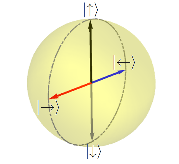
(a) Depiction of the Bloch sphere.

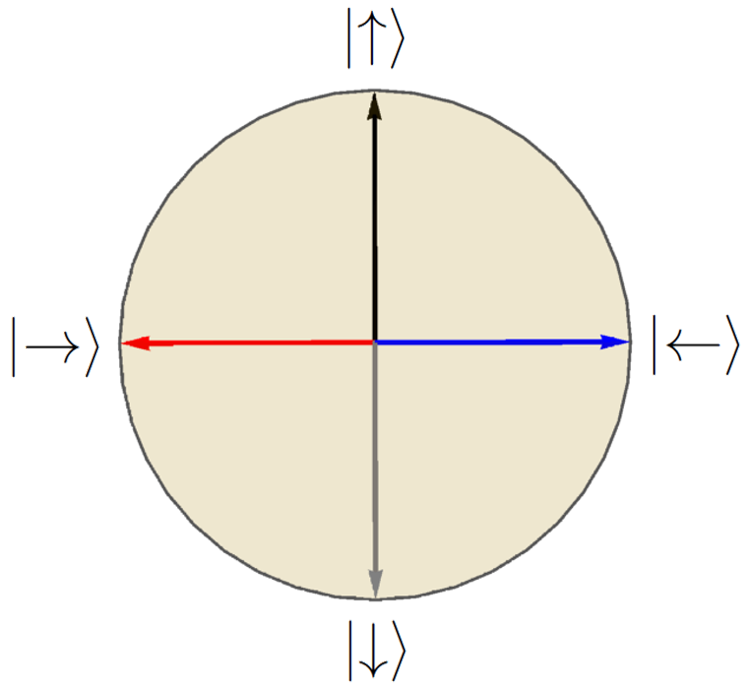
(b) Cross-section of the Bloch sphere.

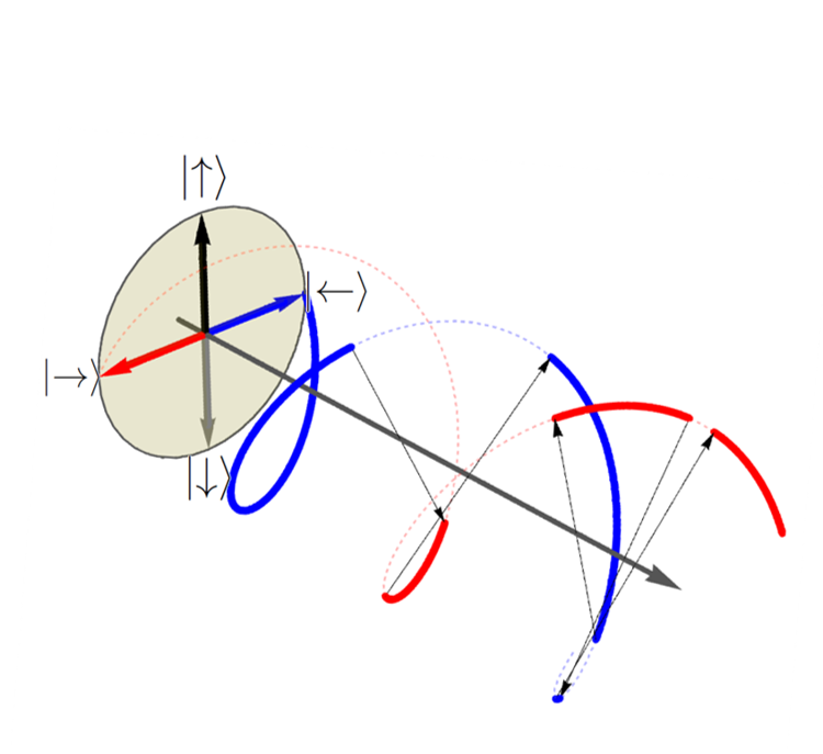
(c) An ontic trajectory.

Figure 1:

A spin-1/2 system has a two-dimensional Hilbert space whose rays can be visualized as points on the surface of a sphere of unit radius, known as the Bloch sphere (see Figure 1a), according to the following parametrization:

$$|\Psi\rangle=\cos\frac{\theta}{2}|\uparrow\rangle+e^{i\phi}\sin\frac{\theta}{2}|\downarrow\rangle,\qquad 0\leq\theta\leq\pi,\quad 0\leq\phi<2\pi.$$ (24)

This expression is the most general formula for a unit-norm vector in a two-dimensional complex Hilbert space, up to irrelevant overall phase. Antipodal points represent orthogonal states—states of opposite spin.

Consider the circular slice of the Bloch sphere depicted in Figure 1b, with spin right/left along the $x$-axis and spin up/down along the $z$-axis. Let the unitary evolution of the ontic basis smoothly and steadily rotate an axis through the Bloch sphere that is initially aligned with the $x$-axis. We can visualize this set-up in terms of a cylinder $S^{1}\times\mathbb{R}$, where $\mathbb{R}$ refers to time, and mark the points at antipodal ends as they trace out a double helix—the shape of the trajectories of the possible ontic states of the system. These helical trajectories are depicted as red and blue dotted curves in Figure 1c.

The actual ontic trajectory can hop between the two strands of this double helix. There can be hops at every instant in time (so the trajectory can be nowhere continuous), but, for visualization purposes, imagine that it spends finite time intervals on alternating strands. One such trajectory is depicted as solid colored red and blue curves segments in Figure 1c. The jumps are depicted as thin black arrows crossing from one possible ontic trajectory to the other.

4.3 Unitary Evolution and Closed-System Ontic Dynamics

The dynamics of a system’s density matrix is linked to the dynamics of the underlying ontic state of the system through our quantum conditional probabilities (7), which again are well-defined to the extent that the system’s overall evolution is at least approximately linear CPTP. These conditional probabilities constrain the ontic dynamics. The most straightforward example of such a constraint arises in the familiar, idealized case of a perfectly closed system whose exact evolution is given by a unitary operator $\hat{U}\mathopen{}\mathclose{{}\left(t^{\prime},t}\right)$. In the usual Schrödinger picture, the state of the system is given by a time-dependent, normalized vector in the system’s Hilbert space such that

$$|\Psi\mathopen{}\mathclose{{}\left(t^{\prime}}\right)\rangle=\hat{U}\mathopen{}\mathclose{{}\left(t^{\prime},t}\right)|\Psi\mathopen{}\mathclose{{}\left(t}\right)\rangle.$$ (25)

At any choice of $t^{\prime}$, we can extend the state vector $|\Psi\mathopen{}\mathclose{{}\left(t^{\prime}}\right)\rangle$ to a (non-unique) set of orthogonal states $\mathopen{}\mathclose{{}\left\{|\Psi_{k}\mathopen{}\mathclose{{}\left(t^{\prime}}\right)\rangle}\right\}_{k}$ that collectively correspond to the set of eigenstates of a degenerate density matrix, with $|\Psi_{1}\mathopen{}\mathclose{{}\left(t^{\prime}}\right)\rangle\equiv|\Psi\mathopen{}\mathclose{{}\left(t^{\prime}}\right)\rangle$. In this case, the first eigenvalue of this density matrix is 1 and the rest vanish, representing the fact that there is no objective uncertainty as to the state of the system.

We have thus already described the ontic dynamics of this system—namely, it never jumps to any other possible ontic state. The quantum conditional probabilities automatically reflect this condition:

$$p\mathopen{}\mathclose{{}\left(\Psi;t^{\prime}|\Psi;t}\right) =\textrm{Tr}\mathopen{}\mathclose{{}\left[\mathopen{}\mathclose{{}\left|\Psi\mathopen{}\mathclose{{}\left(t^{\prime}}\right)\mathopen{}\mathclose{{}\left\rangle}\right\langle\Psi\mathopen{}\mathclose{{}\left(t^{\prime}}\right)}\right|\mathcal{E}^{t^{\prime}\leftarrow t}\mathopen{}\mathclose{{}\left\{\mathopen{}\mathclose{{}\left|\Psi\mathopen{}\mathclose{{}\left(t}\right)\mathopen{}\mathclose{{}\left\rangle}\right\langle\Psi\mathopen{}\mathclose{{}\left(t}\right)}\right|}\right\}}\right]$$

$$=\textrm{Tr}\mathopen{}\mathclose{{}\left[\mathopen{}\mathclose{{}\left|\Psi\mathopen{}\mathclose{{}\left(t^{\prime}}\right)\mathopen{}\mathclose{{}\left\rangle}\right\langle\Psi\mathopen{}\mathclose{{}\left(t^{\prime}}\right)}\right|\hat{U}\mathopen{}\mathclose{{}\left(t^{\prime},t}\right)\mathopen{}\mathclose{{}\left|\Psi\mathopen{}\mathclose{{}\left(t}\right)\mathopen{}\mathclose{{}\left\rangle}\right\langle\Psi\mathopen{}\mathclose{{}\left(t}\right)}\right|\hat{U}^{\dagger}\mathopen{}\mathclose{{}\left(t^{\prime},t}\right)}\right]$$

$$=1.$$

By a similar quick calculation, we find $p\mathopen{}\mathclose{{}\left(\Psi_{k\neq 1};t^{\prime}|\Psi;t}\right)=0$.

The time interval in question can be made as small or large as desired given the idealized assumptions about the system being closed and unitarily evolving, so the only ontic trajectory available in this case is the one that tracks the state vector $|\Psi\mathopen{}\mathclose{{}\left(t^{\prime}}\right)\rangle$ in the system’s Hilbert space. This unitary case is the unique scenario for which there is no uncertainty as to the ontic trajectory of the system.

4.4 Perfectly Linear CPTP Evolution

In order to examine the more general case of linear CPTP evolution, we begin by considering a closed and therefore unitarily evolving parent system $W=S+E$ that we decompose into a subject system $S$ and an environment $E$. We can always decompose the density matrix of $W$ in the following manner:

$$\hat{\rho}_{W}=\hat{\rho}_{S}\otimes\hat{\rho}_{E}+\hat{\sigma}_{SE}.$$ (26)

Here the respective density matrices $\hat{\rho}_{S}$ and $\hat{\rho}_{E}$ for the two subsytems $S$ and $E$ are defined as usual by the appropriate partial traces

$$\hat{\rho}_{S}=\textrm{Tr}_{E}\mathopen{}\mathclose{{}\left[\hat{\rho}_{W}}\right],\quad\hat{\rho}_{E}=\textrm{Tr}_{S}\mathopen{}\mathclose{{}\left[\hat{\rho}_{W}}\right],$$ (27)

and the correlation operator $\hat{\sigma}_{SE}$, which we can take to be defined by $\hat{\rho}_{W}-\hat{\rho}_{S}\otimes\hat{\rho}_{E}$, has vanishing partial traces over $S$ and $E$ by construction and captures the correlations, both classical and quantum, between the systems $S$ and $E$ [23, 24]. For the present discussion, we assume that there was an instant at which there were no correlations between the subsystems and set that as the initial time $t=0$:

$$\hat{\rho}_{W}\mathopen{}\mathclose{{}\left(0}\right)=\hat{\rho}_{S}\mathopen{}\mathclose{{}\left(0}\right)\otimes\hat{\rho}_{E}\mathopen{}\mathclose{{}\left(0}\right).$$ (28)

Given such an initially uncorrelated parent density matrix, the unitary evolution of the parent system reduces to linear CPTP evolution of the subsystems. In particular, the linear CPTP evolution of $S$ is given by the map

$$\mathcal{E}_{S}^{t\leftarrow 0}\mathopen{}\mathclose{{}\left\{\hat{\rho}_{S}\mathopen{}\mathclose{{}\left(0}\right)}\right\}=\textrm{Tr}_{E}\mathopen{}\mathclose{{}\left[\hat{U}_{W}\mathopen{}\mathclose{{}\left(t}\right)\hat{\rho}_{S}\mathopen{}\mathclose{{}\left(0}\right)\otimes\hat{\rho}_{E}\mathopen{}\mathclose{{}\left(0}\right)\hat{U}_{W}^{\dagger}\mathopen{}\mathclose{{}\left(t}\right)}\right]=\sum_{\mathclap{e,e^{\prime}}}\hat{E}_{ee^{\prime}}\mathopen{}\mathclose{{}\left(t}\right)\hat{\rho}_{S}\mathopen{}\mathclose{{}\left(0}\right)\hat{E}_{ee^{\prime}}^{\dagger}\mathopen{}\mathclose{{}\left(t}\right),$$ (29)

where $\hat{U}_{W}\mathopen{}\mathclose{{}\left(t}\right)\equiv\hat{U}_{W}\mathopen{}\mathclose{{}\left(t,0}\right)$ is the unitary evolution operator for the parent system $W$. The summation appearing on the right-hand side of (29) is known as the Kraus decomposition of $\mathcal{E}_{S}^{t\leftarrow 0}$, and the Kraus operators $\hat{E}_{ee^{\prime}}\mathopen{}\mathclose{{}\left(t}\right)$ are defined by

$$\hat{E}_{ee^{\prime}}\mathopen{}\mathclose{{}\left(t}\right)\equiv\sqrt{p_{e}\mathopen{}\mathclose{{}\left(0}\right)}\mathopen{}\mathclose{{}\left\langle e^{\prime};0\mathopen{}\mathclose{{}\left|\hat{U}_{W}\mathopen{}\mathclose{{}\left(t}\right)}\right|e;0}\right\rangle,$$ (30)

where $\mathopen{}\mathclose{{}\left\{|e;t\rangle}\right\}_{e}$ is the system $E$’s set of density-matrix eigenstates at time $t$.

We arrive at some critical observations.

1. The linear CPTP evolution map $\mathcal{E}_{S}^{t\leftarrow 0}$ for the subject system $S$ depends on the inital density matrix of the environment $E$:

   $$\hat{\rho}_{E}\mathopen{}\mathclose{{}\left(0}\right)=\sum_{e}p_{e}\mathopen{}\mathclose{{}\left(0}\right)\mathopen{}\mathclose{{}\left|e;0\mathopen{}\mathclose{{}\left\rangle}\right\langle e;0}\right|.$$ (31)

   The definition of $\hat{E}_{ee^{\prime}}\mathopen{}\mathclose{{}\left(t}\right)$ in (30) makes explicit this dependence on the eigenvalues $\mathopen{}\mathclose{{}\left\{p_{e}\mathopen{}\mathclose{{}\left(0}\right)}\right\}_{e}$ and on the eigenstates $\mathopen{}\mathclose{{}\left\{|e;0\rangle}\right\}_{e}$.

2. The evolution map $\mathcal{E}_{S}^{t\leftarrow 0}$ does not in general respect time-translation symmetry. The initial time $t=0$ is special because it is at that particular time that we know that $S$ and $E$ are uncorrelated. In fact, continuous time-translation symmetry would imply that no correlations ever build up between the subsystems and therefore that the unitary evolution of the parent system $W$ factorizes.

3. The evolution map $\mathcal{E}_{S}^{t\leftarrow 0}$ is not reversible in general in the sense of having a well-defined inverse. Nor does there generically exist a linear CPTP evolution map between two arbitrary times $t$ and $t^{\prime}$. The assumed unitarity of the parent system $W$ implies that another linear CPTP evolution map $\mathcal{E}_{S}^{-t\leftarrow 0}$ can be defined to evolve backward in time from the uncorrelated state at $t=0$. However, this evolution map likewise cannot generally be reversed.

These observations also apply to the quantum conditional probabilities that constrain the trajectory of the actual ontic state. These conditional probabilities (a) depend on the initial density matrix of the environment, (b) are not time-translation invariant, and (c) are only generally well-defined for intervals either backward or forward from the initial time $t=0$ when the systems $S$ and $E$ are uncorrelated.

The smoothing out of the actual ontic state’s trajectory over short time intervals provides a concrete illustration of the way that our quantum conditional probabilities constrain such trajectories. Let the subsystem $S$ have the initial density matrix

$$\hat{\rho}_{S}\mathopen{}\mathclose{{}\left(0}\right)=\sum_{s}p_{s}\mathopen{}\mathclose{{}\left(0}\right)\hat{P}\mathopen{}\mathclose{{}\left(s;0}\right),$$ (32)

where each eigenprojector of the initial density matrix is $\hat{P}\mathopen{}\mathclose{{}\left(s;0}\right)=\mathopen{}\mathclose{{}\left|s;0\mathopen{}\mathclose{{}\left\rangle}\right\langle s;0}\right|$. Similarly, at time $t$,

$$\hat{\rho}_{S}\mathopen{}\mathclose{{}\left(t}\right)=\sum_{s^{\prime}}p_{s^{\prime}}\mathopen{}\mathclose{{}\left(t}\right)\hat{P}\mathopen{}\mathclose{{}\left(s^{\prime};t}\right),$$ (33)

where each eigenprojector of the density matrix at time $t$ is $\hat{P}\mathopen{}\mathclose{{}\left(s^{\prime};t}\right)=\mathopen{}\mathclose{{}\left|s^{\prime};t\mathopen{}\mathclose{{}\left\rangle}\right\langle s^{\prime};t}\right|$. Then the quantum conditional probability that the subject system is in the ontic state $|s^{\prime};t\rangle$ at time $t$ given an initial ontic state $|s;0\rangle$ at time $t=0$ is

$$p\mathopen{}\mathclose{{}\left(s^{\prime};t|s;0}\right) =\textrm{Tr}_{S}\mathopen{}\mathclose{{}\left[\hat{P}\mathopen{}\mathclose{{}\left(s^{\prime};t}\right)\mathcal{E}_{S}^{t\leftarrow 0}\mathopen{}\mathclose{{}\left\{\hat{P}\mathopen{}\mathclose{{}\left(s;0}\right)}\right\}}\right]$$

$$=\sum_{\mathclap{e,e^{\prime}}}\textrm{Tr}_{S}\mathopen{}\mathclose{{}\left[\hat{P}\mathopen{}\mathclose{{}\left(s^{\prime};t}\right)\hat{E}_{ee^{\prime}}\mathopen{}\mathclose{{}\left(t}\right)\hat{P}\mathopen{}\mathclose{{}\left(s;0}\right)\hat{E}_{ee^{\prime}}^{\dagger}\mathopen{}\mathclose{{}\left(t}\right)}\right].$$ (34)

In the limit $t\to 0$, we have $\hat{E}_{ee^{\prime}}\mathopen{}\mathclose{{}\left(t}\right)\to\sqrt{p_{e}\mathopen{}\mathclose{{}\left(0}\right)}\delta_{ee^{\prime}}\hat{1}$. Substituting this limiting expression into (34) and carrying out the partial trace over $S$ yields the trivial result

$$\lim_{t\to 0}p\mathopen{}\mathclose{{}\left(s^{\prime};t|s;0}\right)=\sum_{\mathclap{e,e^{\prime}}}p_{e}\mathopen{}\mathclose{{}\left(0}\right)\delta_{ee^{\prime}}\delta_{ss^{\prime}}=\delta_{ss^{\prime}}.$$ (35)

Assuming that the parent system’s evolution is smooth, then when the time $t$ is very close to $t=0$, the conditional probability that the system’s actual ontic state jumps between orthogonal possible ontic states is very small.

Absent any further structure at the level of the parent system’s evolution map, no other quantum conditional probabilities can be defined for the subsystem $S$ that are conditioned solely on information in $S$, and no additional constraints on the actual ontic trajectory of $S$ may be inferred. For example, even if we have a definition of the space of ontic trajectories for the subsystem $S$, the conditional probabilities defined by (34) generally do not tell us much about which particular trajectory the system’s actual ontic state may follow to some final state $|s^{\prime};t\rangle$ at time $t$ given an initial state $|s;0\rangle$. Moreover, one cannot generally subdivide the time interval from $0$ to $t$ into smaller sub-intervals and compute intermediate conditional probabilities in the hopes of establishing some kind of probabilistic measure on the space of ontic trajectories.

To see more concretely what goes wrong, we suppose for our present purposes the existence of a linear CPTP evolution map $\mathcal{E}_{S}^{t_{2}\leftarrow t_{1}}$ from a time $t_{1}>0$ to a later time $t_{2}>t_{1}$ and consider the composition of the two evolution maps $\mathcal{E}_{S}^{t_{1}\leftarrow 0}$ and $\mathcal{E}_{S}^{t_{2}\leftarrow t_{1}}$. Introducing a convenient multi-index $\alpha\equiv\mathopen{}\mathclose{{}\left(e,e^{\prime}}\right)$, and denoting by $\mathopen{}\mathclose{{}\left\{\hat{E}_{\alpha}^{t_{2}\leftarrow t_{1}}}\right\}_{\alpha}$ the Kraus operators corresponding to the evolution map $\mathcal{E}_{S}^{t_{2}\leftarrow t_{1}}$, we expand the composition of the two evolution maps in terms of their respective Kraus decompositions:

$$\mathcal{E}_{S}^{t_{2}\leftarrow t_{1}}\mathopen{}\mathclose{{}\left\{\mathcal{E}_{S}^{t_{1}\leftarrow 0}\mathopen{}\mathclose{{}\left\{\hat{\rho}_{S}\mathopen{}\mathclose{{}\left(0}\right)}\right\}}\right\} =\sum_{\alpha}\mathcal{E}_{S}^{t_{2}\leftarrow t_{1}}\mathopen{}\mathclose{{}\left\{\hat{E}_{\alpha}^{t_{1}\leftarrow 0}\hat{\rho}_{S}\mathopen{}\mathclose{{}\left(0}\right)\mathopen{}\mathclose{{}\left(\hat{E}_{\alpha}^{t_{1}\leftarrow 0}}\right)^{\dagger}}\right\}$$

$$=\sum_{\mathclap{\alpha,\beta}}\hat{E}_{\beta}^{t_{2}\leftarrow t_{1}}\hat{E}_{\alpha}^{t_{1}\leftarrow 0}\hat{\rho}_{S}\mathopen{}\mathclose{{}\left(0}\right)\mathopen{}\mathclose{{}\left(\hat{E}_{\alpha}^{t_{1}\leftarrow 0}}\right)^{\dagger}\mathopen{}\mathclose{{}\left(\hat{E}_{\alpha}^{t_{2}\leftarrow t_{1}}}\right)^{\dagger}.$$ (36)

Comparing (36) with the correct evolution according to the single evolution map $\mathcal{E}_{S}^{t_{2}\leftarrow 0}$ from $0\to t_{2}$,

$$\mathcal{E}_{S}^{t_{2}\leftarrow 0}\mathopen{}\mathclose{{}\left\{\hat{\rho}_{S}\mathopen{}\mathclose{{}\left(0}\right)}\right\}=\sum_{\alpha}\hat{E}_{\alpha}^{t_{2}\leftarrow 0}\hat{\rho}_{S}\mathopen{}\mathclose{{}\left(0}\right)\mathopen{}\mathclose{{}\left(\hat{E}_{\alpha}^{t_{2}\leftarrow 0}}\right)^{\dagger},$$ (37)

we note that the Kraus operators in these two expressions do not agree. This mismatch is a symptom of the fact that composition of linear CPTP evolution operators does not generically obey the semigroup property

$$\mathcal{E}_{S}^{t_{2}\leftarrow t_{1}}\mathcal{E}_{S}^{t_{1}\leftarrow 0}=\mathcal{E}_{S}^{t_{2}\leftarrow 0}.$$ (38)

The failure of generic linear CPTP evolution to satisfy (38) means that we cannot safely define a measure on a system’s space of ontic trajectories by subdividing finite time intervals into infinitesimal pieces and chaining together corresponding conditional probabilities in a manner analogous to Feynman’s formulation of path integrals for quantum theory.

Thus, in general, even when a parent system has perfectly unitary dynamics, the dynamics of its subsystems can be so unconstrained that their actual ontic trajectories remain hidden. Subsystem dynamics cannot even be assumed to provide a probabalistic measure on the space of ontic trajectories, thereby implying a deeper level of uncertainty than is usually explicitly considered in physics. Yet, despite its unfamiliarity, there is nothing illogical about such non-probabilistic uncertainty. Indeed, it rests on weaker assumptions than probabilistic uncertainty.

There is a connection between the hidden nature of the actual ontic state of an entangled subsystem and the hidden nature of its trajectories. When a system is entangled with its environment, the minimal modal interpretation asserts that the system’s actual ontic state is one of the eigenstates of its density matrix (Axioms 1 and 2). However, the minimal modal interpretation does not tell us which eigenstate is actualized—this information is hidden from all possible observers. For nontrivial linear CPTP evolution, a system initially uncorrelated with its environment will begin to build up environmental correlations. Just as entanglement fundamentally masks the instantaneous actual ontic state of a system, these evolving correlations mask the details of the system’s ontic trajectory as the system evolves away from its initially uncorrelated state. We conjecture that our quantum conditional probabilities represent the maximal amount of information that can be gleaned regarding these ontic trajectories for general situations governed by a well-defined, linear CPTP evolution map. Of course, as we have seen, more information may be available in certain special situations, such as the case of unitary evolution. We turn now to a more general case in which extra information regarding ontic trajectories is available.

4.5 Markovian Evolution

Consider again the parent system $W=S+E$ of the previous section, but now suppose that there is a specific time $t_{1}$ at which the parent system state has ‘forgotten’ the correlations between the subject system and the environment:

$$\hat{\rho}_{W}\mathopen{}\mathclose{{}\left(t_{1}}\right)=\hat{\rho}_{S}\mathopen{}\mathclose{{}\left(t_{1}}\right)\otimes\hat{\rho}_{E}\mathopen{}\mathclose{{}\left(t_{1}}\right).$$ (39)

In this case, we could define linear CPTP evolution for the subsystem $S$ starting at this instant $t_{1}$ in terms of the parent system’s unitary evolution. Self-consistency will then imply the semigroup property (38).

Expanding on this observation, we see that if the parent system’s dynamics sets a natural time scale $\delta t_{S}$ beyond which correlations are periodically mostly erased, then coarse-grained dynamical maps exist that approximately compose over adjacent time intervals and are therefore effectively Markovian. As an illustrative example, imagine a subject system $S$ that is interacting with a bath of photons. The photons can be thought of as ‘pinging’ against the subject system, becoming entangled with it, and then rapidly flying off. The local environment $E$ thereby loses its memory of the subject system’s evolution history and the overall state of the parent system $W=S+E$ approximately re-factorizes. This idea has been fruitfully applied in many areas of physics, and in particular underpins the Lindblad equation, which provides a differential description of such Markovian open-system dynamics [25, 26, 27].

The actual ontic trajectory of a system under such circumstances is still non-probabilistically uncertain for time intervals shorter than $\delta t_{S}$. But one can define coarse-grained trajectories whose uncertainty is captured by products of conditional probabilities at each time-step.

To be explicit, suppose that we have an $N$-state quantum system for which we consistently enumerate the possible ontic states as 1 through $N$. Let $\Delta t\gg\delta t_{S}$ be the coarse-graining time interval, let $t_{0}$ be an initial time, and let

$$t_{n}=t_{0}+n\Delta t$$

be a time at which the system’s actual ontic state is the possible ontic state labeled by $i_{n}\in\mathopen{}\mathclose{{}\left\{1,\ldots,N}\right\}$. We envision a coarse-grained version of ontic jumps potentially taking place during the transition times $\Delta t$. In the present context, there is an approximately well-defined quantum conditional probability $p\mathopen{}\mathclose{{}\left(i_{n};t_{n}|i_{n-1};t_{n-1}}\right)$ for the system to be in the actual ontic state $i_{n}$ at time $t_{n}$ given that its actual ontic state was $i_{n-1}$ at time $t_{n-1}$. Given a sequence of such actual ontic states at particular coarse-grained times $\mathopen{}\mathclose{{}\left\{\mathopen{}\mathclose{{}\left(i_{n};t_{n}}\right)}\right\}_{n=0}^{M}$, the probability associated with this overall coarse-grained ontic trajectory is

$$p_{\mathopen{}\mathclose{{}\left\{i_{k}}\right\}}=\prod_{\mathclap{n=1}}^{M}p\mathopen{}\mathclose{{}\left(i_{n};t_{n}|i_{n-1};t_{n-1}}\right).$$ (40)

This description of coarse-grained ontic trajectories is in keeping with the literature on quantum trajectories associated with the Lindblad equation and other related types of open-system dynamics [27, 28].

The coarse-grained trajectories described here recapitulate the form of the exact ontic trajectories of Section 4.2. The crucial difference, again, is that whereas we have been able to define a measure (40) on our coarse-grained trajectories, no measure can be placed a priori on the space of exact ontic trajectories during a finite time interval. Having the additional structure of approximate Markovianity over a dynamically determined coarse-graining time scale allows for a somewhat more smoothed-out picture of approximate ontic trajectories.

4.6 More General Evolution

It turns out that linear CPTP evolution is not sufficiently general to capture every possible kind of open-system dynamics. Indeed, open-system dynamics need not even be linear.^,

To make this point clear with an explicit example, consider a parent system $W=S+E$ with subsystems $S$ and $E$ that may never be uncorrelated, and let $\mathcal{E}_{W}^{t^{\prime}\leftarrow t}$ be a linear CPTP map for the parent system $W$, where we leave open the possibility that this map may be unitary. The density matrix for the subsystem $S$ at time $t^{\prime}$ is then given by

$$\hat{\rho}_{S}\mathopen{}\mathclose{{}\left(t^{\prime}}\right)=\textrm{Tr}_{E}\mathopen{}\mathclose{{}\left[\hat{\rho}_{W}\mathopen{}\mathclose{{}\left(t^{\prime}}\right)}\right]=\textrm{Tr}_{E}\mathopen{}\mathclose{{}\left[\mathcal{E}_{W}^{t^{\prime}\leftarrow t}\mathopen{}\mathclose{{}\left\{\hat{\rho}_{W}\mathopen{}\mathclose{{}\left(t}\right)}\right\}}\right],$$ (41)

which is not generically a linear (or even an analytic) function of the density matrix of the subsystem $S$ at the initial time $t$, due to the possible presence of entanglement between the subsystems $S$ and $E$. Denoting by $\hat{P}_{W}\mathopen{}\mathclose{{}\left(w;t}\right)$ each eigenprojector of $\hat{\rho}_{W}\mathopen{}\mathclose{{}\left(t}\right)$ and denoting by $\hat{P}_{S}\mathopen{}\mathclose{{}\left(s^{\prime};t^{\prime}}\right)$ each eigenprojector of $\hat{\rho}_{S}\mathopen{}\mathclose{{}\left(t^{\prime}}\right)$, we see that the quantum conditional probabilities constraining ontic trajectories of $S$ in this more general case explicitly depend on the state of the parent system $W$:

$$p_{S|W}\mathopen{}\mathclose{{}\left(s^{\prime};t^{\prime}|w;t}\right)=\textrm{Tr}_{W}\mathopen{}\mathclose{{}\left[\mathopen{}\mathclose{{}\left(\hat{P}_{S}\mathopen{}\mathclose{{}\left(s^{\prime};t^{\prime}}\right)\otimes\hat{1}_{E}}\right)\mathcal{E}_{W}^{t^{\prime}\leftarrow t}\mathopen{}\mathclose{{}\left\{\hat{P}_{W}\mathopen{}\mathclose{{}\left(w;t}\right)}\right\}}\right].$$ (42)

Quantum entanglement at the initial time $t$ precludes us from factorizing the eigenprojectors $\hat{P}_{W}\mathopen{}\mathclose{{}\left(w;t}\right)$ of the parent system’s density matrix into a tensor product of eigenprojectors of the respective density matrices of the subsystems $S$ and $E$.

In the absence of entanglement at the initial time $t$, this factorization can indeed be carried out and we have

$$\hat{P}_{W}\mathopen{}\mathclose{{}\left(w=(s,e);t}\right)=\hat{P}_{S}\mathopen{}\mathclose{{}\left(s;t}\right)\otimes\hat{P}_{E}\mathopen{}\mathclose{{}\left(e;t}\right).$$ (43)

Then (42) becomes

$$p_{S|W}\mathopen{}\mathclose{{}\left(s^{\prime};t^{\prime}|w;t}\right) =\textrm{Tr}_{W}\mathopen{}\mathclose{{}\left[\mathopen{}\mathclose{{}\left(\hat{P}_{S}\mathopen{}\mathclose{{}\left(s^{\prime};t^{\prime}}\right)\otimes\hat{1}_{E}}\right)\mathopen{}\mathclose{{}\left(\mathcal{E}_{W}^{t^{\prime}\leftarrow t}\mathopen{}\mathclose{{}\left\{\hat{P}_{S}\mathopen{}\mathclose{{}\left(s;t}\right)\otimes\hat{P}_{E}\mathopen{}\mathclose{{}\left(e;t}\right)}\right\}}\right)}\right]$$

$$=\textrm{Tr}_{S}\mathopen{}\mathclose{{}\left[\hat{P}\mathopen{}\mathclose{{}\left(s^{\prime};t^{\prime}}\right)\mathcal{E}_{S|E,e}^{t^{\prime}\leftarrow t}\mathopen{}\mathclose{{}\left\{\hat{P}_{S}\mathopen{}\mathclose{{}\left(s;t}\right)}\right\}}\right]$$

$$=p_{S|E,e}\mathopen{}\mathclose{{}\left(s^{\prime};t^{\prime}|(s,e);t}\right),$$ (44)

where

$$\mathcal{E}_{S|E,e}^{t^{\prime}\leftarrow t}\mathopen{}\mathclose{{}\left\{\hat{P}_{S}\mathopen{}\mathclose{{}\left(s;t}\right)}\right\}\equiv\textrm{Tr}_{E}\mathopen{}\mathclose{{}\left[\mathcal{E}_{W}^{t^{\prime}\leftarrow t}\mathopen{}\mathclose{{}\left\{\hat{P}_{S}\mathopen{}\mathclose{{}\left(s;t}\right)\otimes\hat{P}_{E}\mathopen{}\mathclose{{}\left(e;t}\right)}\right\}}\right]$$ (45)

is the time-evolution map for the subsystem $S$ conditioned on the state $e$ of the environment $E$ at time $t$ at which the two subsystems are not entangled. The conditional-probability formula (44) is analogous to the classical case, for which the probability of the system occupying a particular ontic state at a later time is conditioned on the joint state of the two subsystems at an earlier time. By summing over all environment states $e$, and using the resolution of the identity $\sum_{e}\hat{P}_{E}\mathopen{}\mathclose{{}\left(e;t}\right)=\hat{1}_{E}$, we arrive at a linear CPTP map $\mathcal{E}_{S}^{t^{\prime}\leftarrow t}$ describing the evolution of $S$ without any reference to the environment. So we see that linear dynamics at the level of a parent system descends to linear dynamics for a subsystem when that subsystem is not entangled with other subsystems.

Even in the restricted case in which the parent system’s time-evolution map factorizes,

$$\mathcal{E}_{W}^{t^{\prime}\leftarrow t}=\mathcal{E}_{S}^{t^{\prime}\leftarrow t}\otimes\mathcal{E}_{E}^{t^{\prime}\leftarrow t},$$ (46)

the evolution map (41) does not generically yield a linear mapping at the level of the subsystem $S$. Entanglement is therefore responsible for a uniquely quantum obstruction to the existence of exactly linear CPTP open-system dynamics. This obstruction represents a novel, purely quantum form of uncertainty that arises at the level of ontic dynamics even when the subsystems are not dynamically coupled in the sense of (46).

5 Conclusion

5.1 Measurement and Ontic Trajectories

To what extent can we say anything about the ontic trajectory of a quantum system during a typical von Neumann-type measurement interaction? Recalling the simple model of Section 3.2, we assume that the subject system is prepared in a state vector $|\Psi\rangle$ and that the measurement apparatus and environment are both initially uncorrelated with the subject system. We further assume for simplicity that the parent system evolves unitarily, with decoherence arising through the entangling of the subject system with its environment. These features of our simple model imply that we are in the scenario described by Section 4.4—the subsystem of interest evolves according to a linear CPTP map. We see that during the measurement’s short—but finite—span of time, there are no stringent constraints on the subject system’s underlying ontic dynamics other than that the subject system ends up in an actual ontic state very close to one of the measurement eigenstates.

Of course, we can cut the measurement process off shortly after it starts. In that eventuality, our quantum conditional probabilities dictate that the subject system’s actual ontic state will likely still be quite close to $|\Psi\rangle$. But this fact doesn’t tell us anything about the overall ontic trajectory that the subject system would take if we were instead to let the measurement develop over a sufficiently long period.

Clearly, collapse-like dynamics and the Copenhagen interpretation are successful in practice. From our perspective, this success stems from the rapid rate of decoherence and the generic indivisibility of linear evolution that we described earlier. The minimal modal interpretation threads the needle between, on the one hand, closing the conceptual gap that decoherence leaves open between proper and improper mixtures in standard quantum theory, and, on the other hand, saying too much about the underlying dynamics of ontic states. The role of fundamental, non-probabilistic uncertainty in masking ontic trajectories is crucial to the consistency of the interpretation and its minimal modifications to the standard foundational axioms of quantum theory.

5.2 Classical vs. Quantum Ontic Trajectories

The classical and quantum ontic trajectories discussed in Section 4.2 are quite similar. The classical space of ontic trajectories for an $N$-state system is $\mathbb{Z}_{N}\times\mathbb{R}$, corresponding to the assignment of a system state to each instant in time. According to the minimal modal interpretation of quantum theory, the space of ontic trajectories for an $N$-state quantum system is essentially the same space of functions as in the classical case, along with all possible unitary-evolution maps that evolve the basis of possible ontic states within the quantum system’s Hilbert space.

The foregoing kinematical description alone is insufficient for determining conditional probabilities over time without additional assumptions about dynamics. As discussed in Section 4.4, Markovian behavior isn’t generic, even for a quantum system evolving according to linear CPTP dynamics. A new obstruction to Markovianity arises from evolving entanglement between the system in question and its environment. The lack of Markovianity precludes us from defining a measure on the system’s space of ontic trajectories, thereby implying another, deeper level of non-probabilistic uncertainty about the behavior of the system’s actual ontic state.

In Section 4.6, we explored the scenario in which a system and its environment may always feature a significant amount of entanglement. In the presence of such entanglement, the dynamics a subsystem inherits from its parent system governing the subsystem’s density matrix will be nonlinear. Nonlinear evolution obstructs even the definition of quantum conditional probabilities, meaning that the dynamics of the subsystem’s actual ontic state is completely hidden and thus exhibits another manifestation of non-probabilisitc uncertainty.

5.3 Does the Minimal Modal Interpretation Modify Quantum Theory?

We emphasize that the role played by linear CPTP dynamics in the minimal modal interpretation’s axioms is not a fundamental modification of the dynamics of quantum theory. Our interpretation is formulated in recognition of the fact that all physically realistic systems are to some extent open systems and that standard quantum theory exhibits a form of non-reductionism: States of parent systems do not fully determine the states of their subsystems. In the minimal modal interpretation, this non-reductionism translates into system-centric ontology: The ontologies of subsystems do not a priori mesh together in a classically intuitive way that determines the ontology of the parent system. (See Axiom 3.) However, these system-centric ontologies fit together in a more classically coherent manner as systems become macroscopic, as we discuss in more depth in [11] and will explore further in future work.

Appendix A Quantum Conditional Probabilities

In this appendix, we motivate the formula (7) for the quantum conditional probabilities at the heart of the minimal modal interpretation. We start with a parent system $W=Q_{1}+Q_{2}$ partitioned into subsystems $Q_{1}$ and $Q_{2}$ that are mutually disjoint. The reduced density matrix of the subsystem $Q_{1}$ at time $t^{\prime}$ is given by the partial trace

$$\hat{\rho}_{Q_{1}}\mathopen{}\mathclose{{}\left(t^{\prime}}\right)=\textrm{Tr}_{Q_{2}}\mathopen{}\mathclose{{}\left[\hat{\rho}_{W}\mathopen{}\mathclose{{}\left(t^{\prime}}\right)}\right].$$ (47)

The reduced density matrix of the subsystem $Q_{2}$ is similarly defined. At any given time $t$, the density matrices of $W$ and the subsystems $Q_{1}$ and $Q_{2}$ can be expanded in the bases of their respective eigenprojectors $\mathopen{}\mathclose{{}\left\{\hat{P}_{W}\mathopen{}\mathclose{{}\left(w;t}\right)}\right\}_{w}$, $\mathopen{}\mathclose{{}\left\{\hat{P}_{Q_{1}}\mathopen{}\mathclose{{}\left(i_{1};t}\right)}\right\}_{i_{1}},$ and $\mathopen{}\mathclose{{}\left\{\hat{P}_{Q_{2}}\mathopen{}\mathclose{{}\left(i_{2};t}\right)}\right\}_{i_{2}}$:

$$\hat{\rho}_{W}\mathopen{}\mathclose{{}\left(t}\right) =\sum_{w}p_{W}\mathopen{}\mathclose{{}\left(w;t}\right)\hat{P}_{W}\mathopen{}\mathclose{{}\left(w;t}\right),$$ (48)

$$\hat{\rho}_{Q_{1}}\mathopen{}\mathclose{{}\left(t}\right) =\sum_{i_{1}}p_{Q_{1}}\mathopen{}\mathclose{{}\left(i_{1};t}\right)\hat{P}_{Q_{1}}\mathopen{}\mathclose{{}\left(i_{1};t}\right),$$ (49)

$$\hat{\rho}_{Q_{2}}\mathopen{}\mathclose{{}\left(t}\right) =\sum_{i_{2}}p_{Q_{2}}\mathopen{}\mathclose{{}\left(i_{2};t}\right)\hat{P}_{Q_{2}}\mathopen{}\mathclose{{}\left(i_{2};t}\right).$$ (50)

According to the minimal modal interpretation, the probability of the subsystem $Q_{1}$ being in the ontic state $\Psi_{i_{1}}\mathopen{}\mathclose{{}\left(t^{\prime}}\right)$ at time $t^{\prime}$ is

$$p_{Q_{1}}\mathopen{}\mathclose{{}\left(i_{1};t^{\prime}}\right)=\textrm{Tr}_{Q_{1}}\mathopen{}\mathclose{{}\left[\hat{P}_{Q_{1}}\mathopen{}\mathclose{{}\left(i_{1};t^{\prime}}\right)\hat{\rho}_{Q_{1}}\mathopen{}\mathclose{{}\left(t^{\prime}}\right)}\right].$$ (51)

This expression can be rewritten as a formula that explicitly involves the disjoint subsystem $Q_{2}$ and the parent system $W$ by expanding the trace to encompass the entire parent system’s Hilbert space and inserting an identity operator for the Hilbert space of the subsystem $Q_{2}$:

$$p_{Q_{1}}\mathopen{}\mathclose{{}\left(i_{1};t^{\prime}}\right)=\textrm{Tr}_{W}\mathopen{}\mathclose{{}\left[\mathopen{}\mathclose{{}\left(\hat{P}_{Q_{1}}\mathopen{}\mathclose{{}\left(i_{1};t^{\prime}}\right)\otimes\hat{1}_{Q_{2}}}\right)\hat{\rho}_{W}\mathopen{}\mathclose{{}\left(t^{\prime}}\right)}\right].$$ (52)

The identity operator $\hat{1}_{Q_{2}}$ can be expanded in terms of the eigenprojectors $\hat{P}_{Q_{2}}\mathopen{}\mathclose{{}\left(i_{2};t^{\prime}}\right)$,

$$\hat{1}_{Q_{2}}=\sum_{i_{2}}\hat{P}_{Q_{2}}\mathopen{}\mathclose{{}\left(i_{2};t^{\prime}}\right),$$ (53)

and this summation can be pulled out of the trace to yield

$$p_{Q_{1}}\mathopen{}\mathclose{{}\left(i_{1};t^{\prime}}\right)=\sum_{i_{2}}\textrm{Tr}_{W}\mathopen{}\mathclose{{}\left[\mathopen{}\mathclose{{}\left(\hat{P}_{Q_{1}}\mathopen{}\mathclose{{}\left(i_{1};t^{\prime}}\right)\otimes\hat{P}_{Q_{2}}\mathopen{}\mathclose{{}\left(i_{2};t^{\prime}}\right)}\right)\hat{\rho}_{W}\mathopen{}\mathclose{{}\left(t^{\prime}}\right)}\right].$$ (54)

We now suppose that the parent system’s evolution is well-approximated by a linear CPTP map $\mathcal{E}_{W}^{t^{\prime}\leftarrow t}$. Linearity implies that

$$\hat{\rho}_{W}\mathopen{}\mathclose{{}\left(t^{\prime}}\right)=\mathcal{E}_{W}^{t^{\prime}\leftarrow t}\mathopen{}\mathclose{{}\left\{\hat{\rho}_{W}\mathopen{}\mathclose{{}\left(t}\right)}\right\}=\sum_{w}p\mathopen{}\mathclose{{}\left(w;t}\right)\mathcal{E}_{W}^{t^{\prime}\leftarrow t}\mathopen{}\mathclose{{}\left\{\hat{P}_{W}\mathopen{}\mathclose{{}\left(w;t}\right)}\right\},$$ (55)

thereby allowing us to rewrite (54) as

$$p\mathopen{}\mathclose{{}\left(w^{\prime};t^{\prime}}\right)=\sum_{\mathclap{i_{2},w}}\textrm{Tr}_{W}\mathopen{}\mathclose{{}\left[\mathopen{}\mathclose{{}\left(\hat{P}_{Q_{1}}\mathopen{}\mathclose{{}\left(i_{1};t^{\prime}}\right)\otimes\hat{P}_{Q_{2}}\mathopen{}\mathclose{{}\left(i_{2};t^{\prime}}\right)}\right)\mathcal{E}_{W}^{t^{\prime}\leftarrow t}\mathopen{}\mathclose{{}\left\{\hat{P}_{W}\mathopen{}\mathclose{{}\left(w;t}\right)}\right\}}\right]p\mathopen{}\mathclose{{}\left(w;t}\right).$$ (56)

This last expression can be interpreted as a Bayesian propagation formula in its familiar sense,

$$p\mathopen{}\mathclose{{}\left(w^{\prime};t^{\prime}}\right)=\sum_{\mathclap{i_{2},w}}p_{Q_{1},Q_{2}|W}\mathopen{}\mathclose{{}\left(i_{1},i_{2};t^{\prime}|w;t}\right)p\mathopen{}\mathclose{{}\left(w;t}\right),$$ (57)

provided that we adopt Axiom 4 and make the identification

$$p_{Q_{1},Q_{2}|W}\mathopen{}\mathclose{{}\left(i_{1},i_{2};t^{\prime}|w;t}\right)=\textrm{Tr}_{W}\mathopen{}\mathclose{{}\left[\mathopen{}\mathclose{{}\left(\hat{P}_{Q_{1}}\mathopen{}\mathclose{{}\left(i_{1};t^{\prime}}\right)\otimes\hat{P}_{Q_{2}}\mathopen{}\mathclose{{}\left(i_{2};t^{\prime}}\right)}\right)\mathcal{E}_{W}^{t^{\prime}\leftarrow t}\mathopen{}\mathclose{{}\left\{\hat{P}_{W}\mathopen{}\mathclose{{}\left(w;t}\right)}\right\}}\right].$$ (58)

Our last step is not strictly necessary—we choose to interpret the trace formula in (58) as a conditional probability. In keeping with the minimalist spirit of our interpretation of quantum theory, note that we have constructed this new set of conditional probabilities out of standard ingredients without introducing any exotic elements or assumptions.

The conditional probabilities defined by (58) can be generalized to the case of a parent system $W=Q_{1}+\cdots+Q_{n}$ consisting of $n$ disjoint subsystems $Q_{1},\ldots,Q_{n}$ by replacing $Q_{2}\to Q_{2}+\cdots+Q_{n}$ and $\hat{1}_{Q_{2}}\to\hat{1}_{Q_{2}}\otimes\cdots\otimes\hat{1}_{Q_{n}}$. Following steps analogous to those detailed above for the bipartite case, one derives the $n$-subsystem joint conditional probabilities

$$p_{Q_{1},\ldots,Q_{n}|W}\mathopen{}\mathclose{{}\left(i_{1},\text{$\ldots$,}i_{n};t^{\prime}|w;t}\right)=\textrm{Tr}_{W}\mathopen{}\mathclose{{}\left[\mathopen{}\mathclose{{}\left(\hat{P}_{Q_{1}}\mathopen{}\mathclose{{}\left(i_{1};t^{\prime}}\right)\otimes\cdots\otimes\hat{P}_{Q_{n}}\mathopen{}\mathclose{{}\left(i_{n};t^{\prime}}\right)}\right)\mathcal{E}_{W}^{t^{\prime}\leftarrow t}\mathopen{}\mathclose{{}\left\{\hat{P}_{W}\mathopen{}\mathclose{{}\left(w;t}\right)}\right\}}\right].$$ (59)

Of course, in order for these quantities to qualify as proper conditional probabilities, they should be non-negative and sum to unity. What follows is a proof that our quantum conditional probabilities indeed have these properties.

1. Non-negativity: The tensor-product operator

   $$\hat{P}_{Q_{1}}\mathopen{}\mathclose{{}\left(i_{1};t^{\prime}}\right)\otimes\cdots\otimes\hat{P}_{Q_{n}}\mathopen{}\mathclose{{}\left(i_{n};t^{\prime}}\right)$$ (60)

   and the time-evolved projection operator $\mathcal{E}_{W}^{t^{\prime}\leftarrow t}\mathopen{}\mathclose{{}\left\{\hat{P}_{W}\mathopen{}\mathclose{{}\left(w;t}\right)}\right\}$ are both manifestly positive semidefinite. If we call the first positive semidefinite operator $\hat{A}$ and the second $\hat{B}$, then $\sqrt{\hat{A}}$ and $\sqrt{\hat{B}}$ are also positive semidefinite and we have

   $$\textrm{Tr}\mathopen{}\mathclose{{}\left[\hat{A}\hat{B}}\right]=\textrm{Tr}\mathopen{}\mathclose{{}\left[\sqrt{\hat{A}}\sqrt{\hat{A}}\sqrt{\hat{B}}\sqrt{\hat{B}}}\right]=\textrm{Tr}\mathopen{}\mathclose{{}\left[\sqrt{\hat{B}}\sqrt{\hat{A}}\sqrt{\hat{A}}\sqrt{\hat{B}}}\right]=\textrm{Tr}\mathopen{}\mathclose{{}\left[\mathopen{}\mathclose{{}\left(\sqrt{\hat{A}}\sqrt{\hat{B}}}\right)^{\dagger}\mathopen{}\mathclose{{}\left(\sqrt{\hat{A}}\sqrt{\hat{B}}}\right)}\right]\geq 0.$$

   Therefore, our conditional probabilities are non-negative, as claimed:

   $$p_{Q_{1},\ldots,Q_{n}|W}\mathopen{}\mathclose{{}\left(i_{1},\ldots,i_{n};t^{\prime}|w;t}\right)\geq 0.$$ (61)

2. Unit measure: Taking a fixed parent-system ontic state $w$ and summing over all the final subsystem states $i_{1},\ldots,i_{n}$, we find

   $$\sum_{\mathclap{i_{1},\ldots,i_{n}}}p_{Q_{1},\ldots,Q_{n}|W}\mathopen{}\mathclose{{}\left(i_{1},\ldots,i_{n};t^{\prime}|w;t}\right) =\sum_{\mathclap{i_{1},\ldots,i_{n}}}\textrm{Tr}_{W}\mathopen{}\mathclose{{}\left[\mathopen{}\mathclose{{}\left(\hat{P}_{Q_{1}}\mathopen{}\mathclose{{}\left(i_{1};t^{\prime}}\right)\otimes\cdots\otimes\hat{P}_{Q_{n}}\mathopen{}\mathclose{{}\left(i_{n};t^{\prime}}\right)}\right)\mathcal{E}_{W}^{t^{\prime}\leftarrow t}\mathopen{}\mathclose{{}\left\{\hat{P}_{W}\mathopen{}\mathclose{{}\left(w;t}\right)}\right\}}\right]$$

   $$=\textrm{Tr}_{W}\mathopen{}\mathclose{{}\left[\mathopen{}\mathclose{{}\left(\hat{1}_{Q_{1}}\otimes\cdots\otimes\hat{1}_{Q_{n}}}\right)\mathcal{E}_{W}^{t^{\prime}\leftarrow t}\mathopen{}\mathclose{{}\left\{\hat{P}_{W}\mathopen{}\mathclose{{}\left(w;t}\right)}\right\}}\right]$$

   $$=\textrm{Tr}_{W}\mathopen{}\mathclose{{}\left[\mathcal{E}_{W}^{t^{\prime}\leftarrow t}\mathopen{}\mathclose{{}\left\{\hat{P}_{W}\mathopen{}\mathclose{{}\left(w;t}\right)}\right\}}\right]$$

   $$=1.$$

References

- [1] P. A. M. Dirac, The Principles of Quantum Mechanics. Oxford University Press, 1st edition, 1930.
- [2] J. von Neumann and R. T. Beyer, (translator). Mathematical Foundations of Quantum Mechanics. Princeton University Press, 1st edition, 1955.
- [3] G. C. Ghirardi, A. Rimini, and T. Weber, “Unified dynamics for microscopic and macroscopic systems.” Physical Review D, 34(2):470-491, 1986. URL: link.aps.org/pdf/10.1103/PhysRevD.34.470, doi: https://doi.org/10.1103/PhysRevD.34.470.
- [4] D. Bohm, “A Suggested Interpretation of the Quantum Theory in Terms of “Hidden” Variables. I”. Physical Review, 85:166-179, January 1952. URL: http://link.aps.org/doi/10.1103/PhysRev.85.166, doi:10.1103/PhysRev.85.166.
- [5] D. Bohm, “A Suggested Interpretation of the Quantum Theory in Terms of “Hidden” Variables. II”. Physical Review, 85:180-193, January 1952. URL: http://link.aps.org/doi/10.1103/PhysRev.85.180, doi:10.1103/PhysRev.85.180.
- [6] B. S. DeWitt, “Quantum mechanics and reality”. Physics Today, 23(9):30-35, September 1970. URL: http://scitation.aip.org/content/aip/magazine/physicstoday/article/23/9/10.1063/1.3022331, doi:10.1063/ 1.3022331.
- [7] H. Everett III, ““Relative state” formulation of quantum mechanics”. Reviews of Modern Physics, 29(3):454-462, July 1957. URL: http://link.aps.org/doi/10.1103/RevModPhys.29.454, doi:10.1103/RevModPhys.29.454.
- [8] D. Z. Albert, Quantum Mechanics and Experience. Harvard University Press, 1st edition, 1994.
- [9] H. R. Brown and D. Wallace, “Solving the measurement problem: de Broglie-Bohm loses out to Everett”. Foundations of Physics, 35, 2005. URL: http://dx.doi.org/10.1007/s10701-004-2009-3, arXiv:quant-ph/0403094, doi:10.1007/s10701-004-2009-3.
- [10] P. E. Vermaas. A Philosopher’s Understanding of Quantum Mechanics: Possibilities and Impossibilities of a Modal Interpretation. Cambridge University Press, 1999.
- [11] J. A. Barandes and D. Kagan, “The minimal modal interpretation of quantum theory”. arXiv:quant-ph/1405.6755.
- [12] F. Knight, Risk, Uncertainty, and Profit. Hart, Schaffner and Marx. Houghton Mifflin Company, 1921.
- [13] S. Aaronson. “The ghost in the quantum Turing machine”. arXiv:quant-ph/1306.0159.
- [14] W. H. Zurek, “Environment-induced superselection rules.” Physical Review D, 26:1862-1880, 1982. URL: https://journals.aps.org/prd/abstract/10.1103/PhysRevD.26.1862, doi: https://doi.org/10.1103/PhysRevD.26.1862
- [15] J. S. Bell, “On the Einstein-Podolsky-Rosen Paradox”. Physics, 1(3):195-200, 1964.
- [16] J. F. Clauser, M. A. Horne, A. Shimony, and R. A. Holt, “Proposed Experiment to Test Local Hidden-Variable Theories”. Physical Review Letters, 23:880-884, October 1969. URL: http://link.aps.org/doi/10.1103/ PhysRevLett.23.880, doi:10.1103/PhysRevLett.23.880.
- [17] D. M. Greenberger, M. A. Horne, and A. Zeilinger, “Going Beyond Bell’s Theorem”. In Bell’s Theorem, Quantum Theory and Conceptions of the Universe, Fundamental Theories of Physics, pages 69-72. Springer, 1989. URL: 90 http://dx.doi.org/10.1007/978-94-017-0849-4_10, arXiv:0712.0921, doi:10.1007/978-94-017-0849-4_10.
- [18] N. D. Mermin, “Quantum mysteries revisited”. American Journal of Physics, 58(8):731-734, 1990. URL: http: //dx.doi.org/10.1119/1.16503.
- [19] L. Hardy, “Quantum Mechanics, Local Realistic Theories, and Lorentz-Invariant Realistic Theories”. Physical Review Letters, 68:2981-2984, May 1992. URL: http://link.aps.org/doi/10.1103/PhysRevLett.68.2981, doi:10.1103/PhysRevLett.68.2981.
- [20] L. Hardy, “Nonlocality for Two Particles without Inequalities for Almost All Entangled States”. Physical Review Letters, 71:1665-1668, September 1993. URL: http://link.aps.org/doi/10.1103/PhysRevLett.71.1665, doi:10.1103/PhysRevLett.71.1665.
- [21] W. M. Dickson and R. Clifton, “Lorentz-invariance in modal interpretations”. In The Modal Interpretation of Quantum Mechanics, pages 9-47. Springer, 1998. URL: http://link.springer.com/chapter/10.1007/ 978-94-011-5084-2_2.
- [22] W. C. Myrvold, “Modal Interpretations and Relativity”. Foundations of Physics, 32(11):1773-1784, 2002. URL: http://dx.doi.org/10.1023/A%3A1021406924313, arXiv:quant-ph/0209109, doi:10.1023/A:1021406924313.
- [23] P. Stelmachovic and V. Buzek, “Dynamics of open quantum systems initially entangled with environment: Beyond the Kraus representation”. Physical Review A 64, 062106, November 2001. URL: https://arxiv.org/abs/quant-ph/0108136, doi: https://doi.org/10.1103/PhysRevA.64.062106.
- [24] A. Rivas and S. Huelga, Open Quantum Systems: An Introduction. SpringerBriefs in Physics, 2012. URL: https://arxiv.org/abs/1104.5242, doi: https://doi.org/10.1007/978-3-642-23354-8.
- [25] G. Lindblad, “On the Generators of Quantum Dynamical Semigroups". Communications in Mathematical Physics, 48(2):119-130, 1976. URL: http://dx.doi.org/10.1007/BF01608499, doi:10.1007/BF01608499.
- [26] E. Joos, editor. Decoherence and the appearance of a classical world in quantum theory. Springer, 2003.
- [27] K. Hornberger, “Introduction to decoherence theory”. In Entanglement and Decoherence, Springer Lecture Notes in Physics, vol 768, p.221-276, 2009. URL: https://arxiv.org/abs/quant-ph/0612118, doi: https://doi.org/10.1007/978-3-540-88169-8_5 Lindblad (ref 218 big p), ref 195 big p
- [28] M. Esposito and S. Mukamel. “Fluctuation theorems for quantum master equations”. Physical Review E, 73(4):046129, April 2006. URL: http://link.aps.org/doi/10.1103/PhysRevE.73.046129, arXiv:cond-mat/0602679, doi:10.1103/PhysRevE.73.046129.
- [29] D. S. Abrams and S. Lloyd. “Nonlinear quantum mechanics implies polynomial-time solution for NP-complete and #P problems”. Physical Review Letters, 81:3992-3995, November 1998. URL: https://journals.aps.org/prl/abstract/10.1103/PhysRevLett.81.3992, doi: https://doi.org/10.1103/PhysRevLett.81.3992.