Prospects for the detection of electronic pre-turbulence in graphene

Abstract

Based on extensive numerical simulations, accounting for electrostatic interactions and dissipative electron-phonon scattering, we propose experimentally realizable geometries capable of sustaining electronic pre-turbulence in graphene samples. In particular, pre-turbulence is predicted to occur at experimentally attainable values of the Reynolds number between $10$ and $50$, over a broad spectrum of frequencies between $10$ and $100~{}{\rm GHz}$.

\begin{overpic}[width=177.78578pt]{setupB} \put(-8.0,9.0){(a)} \put(50.0,1.0){$L$} \put(47.0,9.5){$W$} \put(71.0,16.0){$d$} \put(68.0,9.5){$D$} \put(20.0,9.7){$w$} \put(34.5,6.4){\scalebox{0.6}{$\blacktriangle$}} \put(34.75,13.9){\scalebox{0.5}{$\blacksquare$}} \end{overpic}

\begin{overpic}[width=177.78578pt]{fig1a} \put(-8.0,11.0){(b)} \put(100.0,17.0){${\bm{v}}({\bm{r}},t)$} \put(100.0,5.0){$\Phi({\bm{r}},t)$} \put(34.5,1.9){\scalebox{0.6}{$\blacktriangle$}} \put(34.75,9.3){\scalebox{0.5}{$\blacksquare$}} \end{overpic}

\begin{overpic}[width=177.78578pt]{fig1b} \put(-8.0,11.0){(c)} \put(100.0,17.0){${\bm{v}}({\bm{r}},t)$} \put(100.0,5.0){$\Phi({\bm{r}},t)$} \put(34.5,1.9){\scalebox{0.6}{$\blacktriangle$}} \put(34.75,9.3){\scalebox{0.5}{$\blacksquare$}} \end{overpic}

\begin{overpic}[width=177.78578pt]{fig1c} \put(-8.0,11.0){(d)} \put(100.0,17.0){${\bm{v}}({\bm{r}},t)$} \put(100.0,5.0){$\Phi({\bm{r}},t)$} \put(34.5,1.9){\scalebox{0.6}{$\blacktriangle$}} \put(34.75,9.3){\scalebox{0.5}{$\blacksquare$}} \end{overpic}

Figure 1: (Color online) Pre-turbulence in high-quality graphene. Panel a) Geometrical details of the setup analyzed in this work. Two graphene leads of width $W=1~{}{\rm\mu m}$ are attached via “funnels” to a central area. Current is injected through an orifice of width $w=0.32~{}{\rm\mu m}$ with an obstacle of length $D=0.3~{}{\rm\mu m}$ placed at a lateral distance $d=0.1~{}{\rm\mu m}$ from the orifice. Panels b)-d) Snapshots of simulations for several values of the injected current. Panel b) Velocity field ${\bm{v}}({\bm{r}},t)$ (top) and electrochemical potential $\Phi({\bm{r}},t)$ (bottom) for an injected current $I=10^{-6}~{}{\rm A}$. Panel c) Same as in panel b) but for an injected current $I=5\cdot 10^{-4}~{}{\rm A}$. Panel d) Same as in panels b) and c) but for $I=10^{-3}~{}{\rm A}$. Data in panels b)-d) have been obtained by setting $\nu=4\times 10^{-4}~{}{\rm m}^{2}/{\rm s}$, $\tau_{\rm D}=50~{}{\rm ps}$, and $C_{\rm g}/e^{2}=1.52\cdot 10^{35}~{}{\rm J}^{-1}{\rm m}^{-2}$ (See the text for definitions of all quantities).

Introduction.—Hydrodynamic theory landaufluidmechanics ; falkovich_book has proven very successful in describing a large variety of physical systems, across a broad range of scales, temperature and density regimes. The ultimate reason of this success is “universality”, namely the insensitivity of the hydrodynamic description to the details of the underlying microscopic physics, as long as such details do not spoil the basic mass, momentum, and energy conservation laws, which underpin the emergence of hydrodynamic behaviour.

Under such conditions, at “sufficiently large” scales (“large” meaning much larger than the typical microscopic interaction length), the specific details of the interactions among the constituent particles do not affect the structure of the hydrodynamic equations, but only the actual values of the transport coefficients controlling dissipative effects, such as the shear and bulk viscosity, as well as the thermal conductivity.

Even if electrons roaming in a crystal can loose energy and momentum towards impurities and the lattice, transport in systems where the mean free path for electron-electron collisions is the shortest length scale of the problem, can also be described by hydrodynamic theory and the Navier-Stokes equations gurzhi_spu_1968 ; dyakonov_prl_1993 ; dyakonov_prb_1995 ; dyakonov_ieee_1996 ; conti_prb_1999 ; govorov_prl_2004 ; muller_prb_2008 ; fritz_prb_2008 ; muller_prl_2009 ; bistritzer_prb_2009 ; mendoza_prl_2011 ; svintsov_jap_2012 ; mendoza_scirep_2013 ; tomadin_prb_2013 ; narozhny_prb_2015 ; briskot_prb_2015 ; torre_prb_2015 ; levitov_naturephys_2016 ; pellegrino_prb_2016 ; principi_prb_2016 ; lucas_prb_2016 ; alekseev_prl_2016 ; falkovich_prl_2017 ; guo_pnas_2017 ; pellegrino_prb_2017 ; levchenko_prb_2017 ; scaffidi_prl_2017 ; delacretaz_prl_2017 ; petrov_arxiv_2018 ; ho_prb_2018 ; lucas_prb_2018_I ; lucas_prb_2018_II . Interestingly, also phonon transport is expected to display hydrodynamic features fugallo_nanolett_2014 ; capellotti_natcomm_2015 .

Recent experiments carried out in high-quality encapsulated graphene sheets bandurin_science_2016 ; kumar_naturephys_2017 ; bandurin_arxiv_2018 ; berdyugin_arxiv_2018 and GaAs quantum wells braem_arxiv_2018 have demonstrated unique qualitative features of hydrodynamic electron transport, namely a negative quasi-local resistance bandurin_science_2016 ; bandurin_arxiv_2018 ; berdyugin_arxiv_2018 ; braem_arxiv_2018 and super-ballistic electron flow kumar_naturephys_2017 , providing, for the first time, the ability to directly measure the dissipative shear viscosity $\eta$ of a two-dimensional (2D) electron system. A different experiment crossno_science_2016 has shown that, near charge neutrality, electron-electron interactions in graphene are strong enough to yield substantial violations of the Wiedemann-Franz law. Evidence of hydrodynamic transport has also been reported in quasi-2D channels of palladium cobaltate moll_science_2016 . For a recent review, see Ref. lucas_jpcm_2018, .

Given this context, it is natural to investigate conditions under which nonlinear terms of the Navier-Stokes equations, which have proven unnecessary so far to explain experimental results bandurin_science_2016 ; kumar_naturephys_2017 ; bandurin_arxiv_2018 ; berdyugin_arxiv_2018 ; braem_arxiv_2018 ; crossno_science_2016 ; moll_science_2016 , may become relevant.

In this Letter, we identify a range of geometrical and physical parameters, in which electronic pre-turbulence can be triggered and sustained in experimentally realizable graphene samples, provided a substantial reduction of electron-phonon scattering is achieved in future experiments. In this context, pre-turbulence refers to a regime prior to the onset of chaos, where periodic oscillations of the velocity field can be observed, without necessarily exhibiting chaotic behaviour kaplan_1979 . To this purpose, we performed extensive numerical simulations taking into account electrostatic interactions and electron-phonon scattering. In particular, we propose suitable geometries for which pre-turbulence: i) occurs at experimentally achievable values of the Reynolds number and, ii) exhibits temporal fluctuations of the electrical potential over a spectrum of frequencies between $10$ and $100~{}{\rm GHz}$.

\begin{overpic}[width=195.12767pt]{dphi-evol}\put(0.0,58.0){(a)} \end{overpic}

\begin{overpic}[width=195.12767pt]{fft-dphi} \put(0.0,58.0){(b)} \end{overpic}

Figure 2: (Color online) (a) Time evolution of the electrochemical potential difference $\Delta\Phi=\Phi(\bar{\bm{r}},t)-\Phi(\bar{\bm{r}}^{\prime},t)$, with $\bar{\bm{r}}=(3~{}\rm{\mu m},0.1~{}\rm{\mu m})$ and $\bar{\bm{r}}^{\prime}=(3~{}\rm{\mu m},0.9~{}\rm{\mu m})$. These two points have been marked in Fig 1a by a triangle ($\bar{\bm{r}}$) and a square ($\bar{\bm{r}}^{\prime}$). Numerical results shown is this figure have been taken from simulations using $\nu=4\times 10^{-4}~{}{\rm m}^{2}/{\rm s}$, $\tau_{\rm D}=50~{}{\rm ps}$, $C_{\rm g}/e^{2}=1.52\cdot 10^{35}~{}{\rm J}^{-1}{\rm m}^{-2}$, and the following values of the injected current: $I=10^{-6}~{}{\rm A}$ (red), $I=5\cdot 10^{-4}~{}{\rm A}$ (green), and $I=10^{-3}~{}{\rm A}$ (blue). (b) Fourier transform of the signals shown in panel (a). The gray vertical lines represent the first ten harmonics of the dominant frequency of the periodic signal obtained from the simulation at injected current $I=5\cdot 10^{-4}~{}{\rm A}$.

Kinetic description and Boltzmann equation.—The direct solution of the Navier-Stokes equations presents a numerically challenging task. In the last decades, it has become apparent that a broad class of complex flows can be addressed by solving suitably simplified lattice versions of Boltzmann’s kinetic equation succi_epl_2015 (for details see Supplementary Material).

For the specific 2D electron system of interest in this work, Boltzmann’s kinetic equation reads as follows:

$$\left(\frac{\partial}{\partial t}+\frac{\bm{p}}{m}\cdot\nabla+\bm{F}\cdot\frac{\partial}{\partial\bm{p}}\right)f=\Omega$$ (1)

where $f(\bm{r},\bm{p},t)$ is the one-particle distribution function expressing the average number of particles in a small element of phase-space centered at position $\bm{r}$ with momentum $\bm{p}$ at time $t$. In the above, $m$ is a suitable effective mass, $\bm{F}$ is the sum of all external forces acting on the system and $\Omega$ is the collision operator, commonly replaced by a relaxation term towards local equilibrium BGK .

It is well known that hydrodynamics emerges from Eq. (S1) in the limit of small Knudsen numbers CE , leading to the continuity, Navier-Stokes, and energy conservation equations. Microscopic details are reflected by the transport coefficients.

The bulk viscosity $\zeta$ is negligibly small for electrons in graphene principi_prb_2016 and while the lattice Boltzmann equation usually features a non-zero value, it has no effect on the physics discussed here since the flow is nearly-incompressible. The shear viscosity $\eta$, on the other hand, plays a crucial role bandurin_science_2016 ; kumar_naturephys_2017 ; bandurin_arxiv_2018 ; berdyugin_arxiv_2018 and consequently it is taken in full account.

For the specific case of 2D electrons in doped graphene, the total force is taken in the following form:

$${\bm{F}}=e\nabla\varphi({\bm{r}},t)-\frac{n({\bm{r}},t)v({\bm{r}},t)}{\tau_{\rm D}}~{}.$$ (2)

The first term at the right-hand side describes electrical forces acting on a fluid element, $-e$ being the elementary charge and $\varphi({\bm{r}},t)$ the electrical potential in the 2D plane where electrons move. The second term describes forces that dissipate electron momentum, i.e. due to collisions between electrons and external agents, such as acoustic phonons in graphene. These are parametrized as an external friction, with a single time scale, i.e. the Drude-like scattering time $\tau_{\rm D}$. This simple parametrization has proven extremely successful in describing experiments in the linear-response regime bandurin_science_2016 ; kumar_naturephys_2017 ; bandurin_arxiv_2018 ; berdyugin_arxiv_2018 ; braem_arxiv_2018 .

Following Ref. tomadin_prb_2013, , we utilize the local capacitance approximation in which the electrical potential is approximated as $\varphi({\bm{r}},t)\approx-e\delta n({\bm{r}},t)/C_{\rm g}$, where $C_{\rm g}$ is the geometrical capacitance of the graphene device of interest and $\delta n({\bm{r}},t)=n({\bm{r}},t)-\bar{n}$, ${\bar{n}}$ being the uniform value of the electron density set by a nearby metallic gate. Using a similar local approximation for the gradient of the pressure Giuliani_and_Vignale , i.e. $\nabla P\approx(\partial P/\partial n)_{n({\bm{r}},t)\to{\bar{n}}}\nabla\delta n({\bm{r}},t)$ we can define the electrochemical potential as $\phi({\bm{r}},t)\equiv-e\delta n({\bm{r}},t)(C^{-1}_{\rm g}+C^{-1}_{\rm Q})$, $C_{\rm Q}=2\bar{n}e^{2}/E_{\rm F}$ being the so-called quantum capacitance Giuliani_and_Vignale and $E_{\rm F}=\hbar v_{\rm F}\sqrt{\pi{\bar{n}}}$ the Fermi energy in single-layer graphene (SLG). Finally, $v_{\rm F}\simeq 10^{6}~{}{\rm m}/{\rm s}$ is the Fermi velocity of massless Dirac fermions in SLG. With reference to Eq. (S1), we use the usual effective mass $m=E_{\rm F}/v^{2}_{\rm F}$ for SLG.

Our numerical results are based on extensive numerical simulations of the geometry shown in Fig. 1a, which can be easily realized experimentally with current technology, and for a large set of values of the relevant physical parameters (see Tab. 1). All cases considered in this work fall in a regime of very small Mach number ${\rm Ma}$, in which compressibility effects can safely be neglected.

The Mach number is defined as the ratio between the plasma-wave velocity $v_{\rm PW}$ and the fluid velocity of the electron fluid, with $v_{\rm PW}=\sqrt{e^{2}\bar{n}v_{\rm F}^{2}/(CE_{\rm F})}$, where $C^{-1}=C_{\rm g}^{-1}+C_{\rm Q}^{-1}$. For the device geometry shown in Fig. 1a and the parameters used in all our simulations, ${\rm Ma}\ll 1$. (This has been explicitly verified a posteriori for all cases. For example, for the simulations corresponding to Figs. 1(b-d), we have ${\rm Ma}\approx 0.0015$, $0.08$, and, $0.12$, respectively.) A small value of ${\rm Ma}$ in turn implies the quasi-incompressibility of the electron fluid. As mentioned earlier on, in this regime we have resorted to a Lattice Boltzmann (LB) approach Succi_book , which, among others, offers the advantage of a comparatively simple handling of non-idealized geometrical boundary conditions. In this work, we use a non-relativistic LB scheme, since relativistic approaches rlbm1 ; rlbm2 ; rlbm3 are appropriate only very close to the charge neutrality point, where charge and energy flows are coupled lucas_jpcm_2018 . Technical details on this numerical approach are reported in Ref. SOM, .

Table 1: Typical values of physical parameters of state of the art experiments compared with those used in our simulations. Refer to Fig. 1a for the definition of $L$ and $W$. All other parameters are defined in the main text.

	Typical experiments	This work
$L$	$5\sim 30~{}\rm{[\mu m]}$	$10~{}\rm{[\mu m]}$
$W$	$1\sim 5~{}\rm{[\mu m]}$	$1~{}\rm{[\mu m]}$
$\bar{n}$	$0.5\sim 4\cdot 10^{12}~{}\rm{[cm^{-2}]}$	$2\cdot 10^{12}~{}\rm{[cm^{-2}]}$
$I$	$10^{-3}\sim 1~{}\rm{[mA]}$	$10^{-3}\sim 1~{}\rm{[mA]}$
$\nu$	$0.01\sim 0.1~{}\rm{[m^{2}/s]}$	$10^{-4}\sim 10^{-3}~{}\rm{[m^{2}/s]}$
$\tau_{\rm D}$	$1\sim 5~{}\rm{[ps]}$	$1\sim 400~{}\rm{[ps]}$
$C_{\rm g}/e^{2}$	$3.03\cdot 10^{34}~{}\rm{[J^{-1}m^{-2}]}$	$3.03\cdot 10^{35}~{}\rm{[J^{-1}m^{-2}]}$

Numerical results.—We consider a geometry close to the one used in recent experimental work kumar_naturephys_2017 , which made use of a constriction to emphasize a clear crossover from the ballistic Sharvin regime to the hydrodynamic regime as a function of temperature. Such geometry is sketched in Fig. 1a, with the addition of a thin linear obstacle, placed in front of the constriction, with the intent of triggering pre-turbulent regimes at low Reynolds numbers.

Fig. 1 qualitatively summarizes our finding. For appropriate values of the transport parameters (low enough kinematic viscosity $\nu=\eta/(nm)$ and large enough $\tau_{\rm D}$) a laminar behaviour is found for low values of the current ($10^{-3}~{}\rm{mA}$, Fig. 1b) injected in the sample. As the value of the injected current is increased ($0.5-1.0~{}\rm{mA}$, Fig. 1c/d, and, correspondingly, the typical fluid element velocity increases), a transition to a pre-turbulent behaviour takes place (identified with a procedure described later in the text).

Present-day experiments cannot map the fluid velocity everywhere in the sample, but typically can only measure the electrochemical potential (also mapped in Fig. 1) at selected sites on the boundaries.

The expected result of such measurements is shown in Fig. 2a, displaying the electrochemical potential difference between locations corresponding to the black square and triangle in Fig. 1a; here again, we appreciate a clear change from a constant to a periodic, to a more irregular trend, which is best analyzed in the frequency domain, see Fig. 2b.

The present simulations cover a wide region in the $\nu$-$\tau_{\rm D}$ plane. Results are collected in Fig. 3, showing the smallest value of $\tau_{\rm D}$ as a function of $\nu$, for which a transition to an observable pre-turbulent regime occurs, denoted by the symbol $\tau^{*}_{\rm D}$.

Points in Fig. 3 refer to experimentally achievable values of the injected current of the order of $\approx 1~{}{\rm mA}$. They have been determined using the onset of a transverse current along the middle section of the device as a discriminating factor; the upper end of these points are simulations for which the root mean square of the transverse current exceeds $1\%$ of the magnitude of the injected current (more details in the Supplementary Material).

Recent works bandurin_science_2016 ; kumar_naturephys_2017 have reported direct experimental measurements of the kinematic viscosity $\nu$ of the 2D electron system in graphene, which are on the order of $\nu\lesssim~{}0.1~{}{\rm m^{2}/s}$. As far as electron-phonon interactions are concerned, state-of-the-art experiments in graphene encapsulated between hexagonal Boron Nitride (hBN) crystals display $\tau_{\rm D}$ ranging between $1$ and $2~{}\rm{ps}$ in the temperature range $70$-$300~{}{\rm K}$, where hydrodynamic behaviour is strongest. Inspection of Fig. 3 may therefore convey disappointing news: for values of the parameters currently achieved in experiments, no pre-turbulent behaviour can be detected. The mitigating observation is that substantial, but not unconceivable, improvements of the transport parameters may eventually turn the picture for good. For example, the viscosity of the electron liquid at elevated injection currents, as those needed to achieve the pre-turbulent regime, is expected to be much smaller than that in the linear-response regime, due to Joule heating deJong_prb_1995 , which notably increases the electron temperature above the lattice temperature. Moreover, recent material science advances stampfer , have enabled much larger values of $\tau_{\rm D}$ than those measured in hBN-encapsulated graphene. Such large values of $\tau_{\rm D}$ can be obtained by using different encapsulating materials, such as ${\rm WSe}_{2}$, which are currently believed to quench scattering of electrons against acoustic phonons in graphene stampfer .

A further encouraging result is that the frequency distribution of the electro-chemical potential falls within a measurable regime, if only with suitably designed experiments.

From a purely fluid-dynamics point of view, it may be interesting to characterize the crossover line clearly shown in Fig. 3 in terms of an appropriate figure of merit. To this purpose, we develop a simplified model, whose starting point is the role played by the Reynolds number as an indicator of turbulence. In the present case, the turbulence-suppressing effect of the dissipative term in the Navier-Stokes equation is augmented by electron-phonon scattering. On purely dimensional grounds, it proves expedient to introduce a modified Reynolds number ${\rm Re^{\prime}}$, incorporating the effect of electron-phonon dissipation, namely:

$${\rm Re^{\prime}}=\frac{|{\bm{v}}|~{}\ell}{\displaystyle\nu+\frac{\ell^{2}}{\tau_{\rm D}}}\quad,$$ (3)

with $|{\bm{v}}|$ a typical fluid-element velocity and $\ell$ a typical length scale for the system at hand.

This very simple model proves adequate to characterize the actual behaviour of the system. Lines in Fig. 3 are level lines for ${\rm Re}^{\prime}$, which capture the trend of the different datasets. In Eq. (3), we use the inlet velocity and obtain $\ell=0.135~{}\rm{\mu m}$ through a linear fit. Such value turns out to be pretty close to the typical geometrical features of the simulated layout.

We obtain the following estimates for the critical modified Reynolds numbers: ${\rm Re^{\prime}}\sim 19$ for $I=10^{-4}~{}\rm{A}$, ${\rm Re^{\prime}}\sim 33$ for $I=5\cdot 10^{-4}~{}\rm{A}$ and ${\rm Re^{\prime}}\sim 47$ for $I=10^{-3}~{}\rm{A}$.

We do not wish to attach any deep meaning to this parametrization, but simply note that it discloses a simple theoretical interpretation of the numerical results.

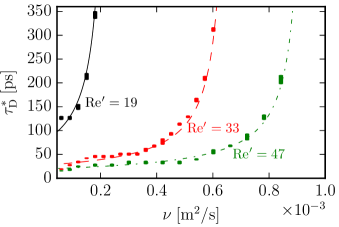
Figure 3: (Color online) Critical value $\tau^{*}_{\rm D}$ of the Drude-like scattering time as a function of the kinematic viscosity $\nu$, for which a transition from a laminar to a pre-turbulent regime is observed. Thick vertical bars represent results of numerical simulations (refer to Ref. SOM, for details on how these intervals are established), with the following values of the injected current: $I=10^{-4}~{}\rm{A}$ (black), $I=5\cdot 10^{-4}~{}\rm{A}$ (red), $I=10^{-3}~{}\rm{A}$ (green). Lines represent iso-Reynolds curves, where ${\rm Re}^{\prime}$ as in Eq. (3) is used in the definition of a Reynolds number that includes extrinsic dissipation due to $\tau_{\rm D}$ and $\ell$ is a fitting parameter. Lines represents fits to the numerical data: $I=10^{-4}~{}\rm{A}$ (solid black line), $I=5\cdot 10^{-4}~{}\rm{A}$ (red dashed line), and $I=10^{-3}~{}\rm{A}$ (green dash-dotted line). Refer to Fig 1a for details on the geometry used in the simulations. Numerical data in this figure have been obtained by setting $C_{\rm g}/e^{2}=3.03\cdot 10^{35}~{}{\rm J}^{-1}{\rm m}^{-2}$.

Closing remarks.—Summarizing, based on extensive numerical simulations, accounting for electrostatic and dissipative effects due to electron-phonon scattering in experimentally realistic geometries, we have identified parameter regimes under which electronic pre-turbulence may eventually be detected by future experiments. To this purpose, such experiments should operate at lower levels of electron-phonon scattering (i.e. $\tau_{\rm D}\sim 20$-$50$ ps) than those that can be achieved in hBN-encapsulated graphene, which is possible by using different encapsulating materials stampfer . As a typical signature of electronic pre-turbulence, we predict electrical potential fluctuations in the frequency range between $10$ and $100~{}{\rm GHz}$, which should be detectable by suitably designed experiments.

We emphasize that the placement of a thin plate across the mainstream electron flow in a constricted channel proves instrumental in lowering the critical Reynolds number at which pre-turbulence occurs. Further optimization may result from a concerted effort between future numerical and experimental investigations.

Acknowledgments.—We wish to thank Andre Geim and Iacopo Torre for useful discussions. A.G. has been supported by the European Union’s Horizon 2020 research and innovation programme under the Marie Sklodowska-Curie grant agreement No. 642069. M.P. is supported by the European Union’s Horizon 2020 research and innovation programme under grant agreement No. 785219 - GrapheneCore2. S.S. acknowledges funding from the European Research Council under the European Union’s Horizon 2020 framework Programme (No. P/2014-2020)/ERC Grant Agreement No. 739964 (COPMAT). The numerical work has been performed on the COKA computing cluster at Università di Ferrara.

Supplementary Information for
“Prospects for the detection of electronic pre-turbulence in graphene”

I Numerical Method

In this section we provide a brief introduction to the Lattice Boltzmann Method (LBM), which has been used to carry out the numerical work presented in the main text. For a thorough introduction to LBM the interested reader in is kindly referred to Succi_book ; Krueger_book .

Lattice Boltzmann methods are a class of numerical fluid-dynamics solvers, initially developed to study quasi-incompressible isothermal fluids higuera-1989 ; chen-1992 ; qian-1993 , and then improved to incorporate e.g. thermo-hydrodynamical fluctuations philippi-2006 ; sbragaglia-2009 ; chikatamarla-2009 , or covering a wider range of fluid velocities from low-velocity to ultra-relativistic regimes mendoza-2010a ; rlbm1 ; rlbm2 . At variance with methods that discretize the Navies-Stokes equations, LBM stems from the mesoscopic Boltzmann equation:

$$\left(\frac{\partial}{\partial t}+\frac{\bm{p}}{m}\cdot\nabla+\bm{F}\cdot\frac{\partial}{\partial\bm{p}}\right)f=\Omega(f)$$ (S1)

where $f(\bm{r},\bm{p},t)$ is the one-particle distribution function expressing the average number of particles in a small element of phase-space centered at position $\bm{r}$ with momentum $\bm{p}$ at time $t$. In the above, $m$ is a suitable effective mass, $\bm{F}$ is the sum of all external forces acting on the system. The collisional operator $\Omega(f)$, describing the changes in $f$ due to particle collisions, is commonly replaced by the single-time relaxation BGK model bhatnagar-1954 :

$$\Omega(f)=\frac{1}{\tau}\left(f^{eq}-f\right)\quad.$$ (S2)

Using this model the evolution of the system is described by a relaxation process, with relaxation time $\tau$, towards a local equilibrium $f^{eq}$ given by the Maxwell-Boltzmann distribution:

$$f^{eq}=n\left(\frac{1}{2\pi k_{B}}\frac{m}{T}\right)\exp{\left(-\frac{1}{2k_{B}}\frac{m}{T}(\bm{\xi}-\bm{u})^{2}\right)}\quad.$$ (S3)

Macroscopic quantities like the particle number density $n(\bm{r},t)$, velocity $\bm{u}(\bm{r},t)$ and temperature $T(\bm{r},t)$ are linked to the microscopic velocity ($\bm{\xi}$) moments of $f$:

$$n(\bm{r},t) =\int f(\bm{r},\bm{\xi},t)\mathop{}\!\mathrm{d}\bm{\xi}$$ (S4)

$$n(\bm{r},t)\bm{u}(\bm{r},t) =\int f(\bm{r},\bm{\xi},t)\bm{\xi}\mathop{}\!\mathrm{d}\bm{\xi}$$ (S5)

$$n(\bm{r},t)T(\bm{r},t) =\frac{1}{2}m\int f(\bm{r},\bm{\xi},t)|\bm{\xi}-\bm{u}(\bm{r},t)|^{2}\mathop{}\!\mathrm{d}\bm{\xi}\quad.$$ (S6)

In the derivation of his 13-moments method, Grad grad-1949 ; grad-1949b made an important observation on the link between the Maxwell-Boltzmann distribution and the Hermite polynomials. In fact, by expanding the equilibrium distribution

$$f^{eq}(\bm{r},\bm{\xi},t)=\omega(\bm{\xi})\sum_{k=0}^{\infty}\frac{1}{k!}a^{(k)}(\bm{r},t)H^{(k)}(\bm{\xi})\quad,$$ (S7)

with $a^{(k)}$ the projection coefficients

$$a^{(k)}(\bm{r},t)=\int f^{eq}(\bm{r},\bm{\xi},t)H^{(k)}(\bm{\xi})\mathop{}\!\mathrm{d}\bm{\xi}\quad,$$ (S8)

and the weighting function $\omega(\bm{\xi})$

$$\omega(\bm{\xi})=\frac{1}{2\pi}\exp{\left(-\frac{1}{2}\bm{\xi}^{2}\right)}\quad,$$ (S9)

it is possible to show that the hydrodynamic variables can be expressed in terms of the low-order Hermite expansion coefficients. The mathematical foundation of the LBM lies on the observation that the Hermite coefficients can be calculated exactly using a Gauss-Hermite quadrature formula, which allows to replace the (continuum) velocity space with a (small) set of discrete velocities $\mathcal{V}=\{\bm{e}_{i}\in\mathbb{R}^{2}\}$ (refer to philippi-2006 ; shan-2016 for the mathematical details).

In this work we have used a iso-thermal version of the D2Q37 philippi-2006 ; sbragaglia-2009 , a fourth-order model, where the order of a model corresponds to the highest retained moment. The stencil is shown in Fig. S1, while in Tab. 1 we detail the velocity vectors and the weights of the quadrature.

Figure S1: Stencil for the D2Q37 model used in the simulations of the main text. Based on the Hermite-Gauss quadrature philippi-2006 ; shan-2016 , the D2Q37 can be regarded as the minimal on grid square lattice exactly recovering the moments of the distribution up to the fourth order.

$\bm{e}_{i}$	$w_{i}$
$\left(\phantom{\pm}0,\phantom{\pm}0\right)_{\rm{\phantom{FS}}}$	$0.2331506691323525$
$\left(\phantom{\pm}0,\pm 1\right)_{\rm{FS}}$	$0.1073060915422190$
$\left(\pm 1,\pm 1\right)_{\rm{FS}}$	$0.0576678598887948$
$\left(\phantom{\pm}0,\pm 2\right)_{\rm{FS}}$	$0.0142082161584507$
$\left(\pm 1,\pm 2\right)_{\rm{FS}}$	$0.0053530490005137$
$\left(\pm 2,\pm 2\right)_{\rm{FS}}$	$0.0010119375926735$
$\left(\phantom{\pm}0,\pm 3\right)_{\rm{FS}}$	$0.0002453010277577$
$\left(\pm 1,\pm 3\right)_{\rm{FS}}$	$0.0002834142529941$
$c_{s}$	0.835436007136204

Table 1: Quadrature weights associated to each velocity group of the D2Q37 stencil. The weights are given with 16 digits to ensure that integrals in Eq.S10 and Eq.S11 are correctly computed at machine precision. Here FS stands for full-symmetric meaning that, for example, $\left(0,\pm 1\right)_{\rm{FS}}$ corresponds to the velocity vectors $\{(0,1),(0,-1),(1,0),(-1,0)\}$. The lattice constant $c_{s}$ is commonly referred to as the speed of sound in the lattice.

Computational Scheme.— For each time step and for each grid site the following operations are performed (see Fig. S1 and Tab. 1 for the definition of the stencil velocities $\bm{e}_{i}$ and the quadrature weights $w_{i}$, $i=0,1,\dots 36$ ):

1. Compute the macroscopic quantities such as density and momentum:

   $$n =\sum_{i=0}^{36}f_{i}$$ (S10)

   $$n\bm{u} =\sum_{i=0}^{36}f_{i}\bm{e}_{i}$$

2. Compute the equilibrium distribution:

   $$f_{i}^{eq}=w_{i}\sum_{k=0}^{4}a^{(k)}H^{(k)}(\bm{e}_{i})\quad.$$ (S11)

3. Evolve the discrete Lattice Boltzmann equation:

   $$f_{i}(\bm{r}+\bm{e}_{i}\Delta t,\bm{e}_{i},t+\Delta t)-f_{i}(\bm{r},\bm{e}_{i},t)=\frac{\Delta t}{\tau}\left(f_{i}^{\rm{eq}}(\bm{r},\bm{e}_{i},t)-f_{i}(\bm{r},\bm{e}_{i},t)\right)+F^{\rm{ext}}_{i}\quad,$$ (S12)

   where $F^{\rm{ext}}_{i}$ is the discrete counterpart of the total external force defined in the main text.

The Chapman Enskog expansion: from from lattice Boltzmann to Navier-Stokes.— Hydrodynamics emerges from Boltzmann’s kinetic theory in the limit of vanishing Knudsen numbers, where the Knudsen number $\rm Kn$ is defined as the ratio between the molecular mean free path and the typical macroscopic length scale. It is therefore natural to think of an expansion of the kinetic equations in powers of a vanishingly small Knudsen number. Such asymptotic analysis can be performed using the Chapman Enskog (CE) expansion. The CE expansion is commonly employed to show that the lattice formulation correctly recovers the Navier-Stokes equations:

$$\partial_{t}n(\bm{r},t)+\partial_{r_{\alpha}}\left(n(\bm{r},t)u_{\alpha}(\bm{r},t)\right) =0$$ (S13)

$$\partial_{t}\left(mn(\bm{r},t)u_{\beta}(\bm{r},t)\right)+mn(\bm{r},t)u_{\beta}(\bm{r},t)\partial_{r_{\alpha}}\left(u_{\alpha}(\bm{r},t)\right) =mn(\bm{r},t)F_{\beta}(\bm{r},t)+\partial_{r_{\alpha}}\sigma_{\alpha\beta}\quad.$$ (S14)

with the stress tensor $\sigma_{\alpha\beta}$ given by

$$\sigma_{\alpha\beta}=\eta(\partial_{\alpha}u_{\beta}+\partial_{\beta}u_{\alpha}-\partial_{\gamma}u_{\gamma}\delta_{\alpha\beta})+\zeta\partial_{\gamma}u_{\gamma}\delta_{\alpha\beta}$$ (S15)

where $\eta$ and $\zeta$ are respectively the shear and the bulk viscosity. In the above, Greek subscripts run over spatial dimensions. The closure of the CE expansion provides the expression of the transport coefficients connecting the microscopic and macroscopic levels. In this work we are mainly interested in the kinematic viscosity:

$$\nu=\frac{\eta}{n~{}m}=c_{s}^{2}\left(\tau-\frac{\Delta t}{2}\right)$$ (S16)

with $c_{s}$ a lattice constant (see Tab. 1). Full details of the CE expansion for the D2Q37 model are reported as Appendix in scagliarini-2010 .

Parameter matching

In an experimental perspective, we are interested in taking measurements of the electrochemical potential. Since this quantity is not a direct observable of the lattice formulation, we need to perform a parameters matching procedure. In the main text we have defined the electrochemical potential as

$$\phi=\varphi(\bm{r})-\frac{\delta P(\bm{r})}{e\bar{n}}~{},$$ (S17)

where $\delta P(\bm{r})=P(\bm{r})-\bar{P}\approx\frac{\epsilon_{\rm F}}{2}\delta n(\bm{r})$. By employing the local capacitance approximation, $\varphi(\bm{r})\approx-e\delta n(\bm{r})/C_{\rm g}$, it is simple to show that an approximation for $\phi$ is given by:

$$\phi=-e\delta n(\bm{r})\left(\frac{1}{C_{\rm g}}+\frac{1}{C_{\rm Q}}\right)~{},$$ (S18)

where $1/C_{\rm Q}=\epsilon_{\rm F}/(2\bar{n}e^{2})$.

As described above, we use a Maxwell-Boltzmann distribution within the LBM formulation. For this reason, it follows that the hydrostatic contribution to the electrochemical potential gives an effective quantum capacitance that can be written as

$$\frac{1}{C_{\rm Q,MB}}=\frac{k_{\rm B}T}{\bar{n}e^{2}}~{}.$$ (S19)

In the numerical scheme, used to describe a iso-thermal dynamic, the temperature appears only in this term. Therefore, using the temperature as an effective parameter, we can match the correct expression for the electrochemical potential:

$$k_{\rm B}T=\frac{\epsilon_{\rm F}}{2}=m\frac{v_{\rm D}^{2}}{2}~{},$$ (S20)

where $m=\epsilon_{\rm F}/v_{\rm D}^{2}$ for single-layer graphene.

To conclude, we stress that the assumptions used in this parameter-matching procedure are valid thanks to the fact that all simulations taken into consideration in this paper work in a quasi-incompressible regime.

II Identifying the crossover between laminar and (pre-)turbulent flow

In Figure 3 of the main text we show, at different values of the kinematic viscosity $\nu$, small intervals for the value of $\tau_{D}^{*}$ for which a crossover from a laminar to a pre-turbulent flow occurs. In order to determine such intervals we have used as a discriminating factor the onset of a transversal current ($u_{y}$) across the middle section of the device. For a given simulation, we have measured at each time step the average value of $<u_{y}(x=L/2,y)>$. We consider the simulated flow to be in a pre-turbulent regime whenever the root mean square of that quantity is larger than $1\%$ of the velocity at the inlet. In Fig. S2 we show an example: the left panel shows, in a qualitative way, the onset of pre-turbulent features in the flow as $\tau_{D}$ is increased; the right panel on the other hand shows the behavior of the root mean square of $<u_{y}(x=L/2,y)>$ as a function of $\tau_{D}$. For this particular example, we see that the crossover occurs in the $\tau_{D}^{*}$ interval $(90~{}\rm{ps},95~{}\rm{ps})$.

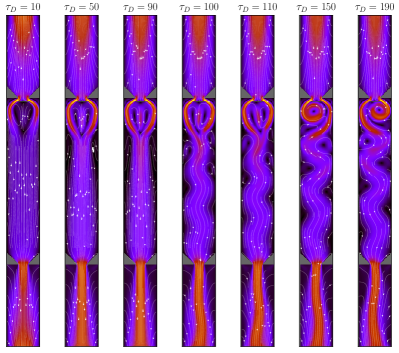
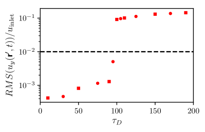
Figure S2: The plot at right shows the ratio between the root mean square transversal velocity along the middle section ($\bm{r^{\prime}}$) of the device and the velocity at the inlet, as a function of $\tau_{D}$. The black ticked line represents the (empirical) threshold used to establish the crossover between a laminar and a pre-turbulent regime. In this example the crossover occurs in the $\tau_{D}^{*}$ interval $(90~{}\rm{ps},95~{}\rm{ps})$. All simulations use an inlet velocity consistent with $I=5\cdot 10^{-4}~{}{\rm A}$ and $\nu=0.45\cdot 10^{-3}\rm{m^{2}/s}$. Squares refer to simulations for which a snapshot of the velocity profile is shown at left; in those profiles we show the velocity streamlines with colors mapping the module of the velocity.

A different criteria that could be employed to quantify the crossover from a laminar to a (pre)-turbulent regime consists in taking into account the vorticity, generally defined as the curl of the velocity (a scalar in the 2D case). In particular, we take into consideration the root mean square (RMS) of the average value of the vorticity. From Fig. S3 we can see that for $\tau_{D}^{*}<90$ the average value of the vorticity is very close to zero, due to the symmetric behavior of the laminar flow; an abrupt change occurs in the interval $\tau_{D}^{*}\in(90~{}\rm{ps},95~{}\rm{ps})$, where the RMS of the average value of the vorticity grows of 6-7 orders of magnitudes. We remark that both methods yield very similar results.

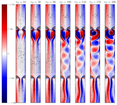
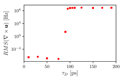
Figure S3: The plot at right shows the root mean square value of the average of vorticity as a function of $\tau_{D}$; we once again observe an abrupt change in the $\tau_{D}^{*}$ interval $(90~{}\rm{ps},95~{}\rm{ps})$ similarly to Fig. S2. All simulations use the same physical parameters as in the previous figure. Squares refer to simulations for which a snapshot of the vorticity profile is shown in the left panel; these profiles show again the velocity streamlines but this time colors map the vorticity profile.

References

- (1) L.D. Landau and E.M. Lifshitz, Course of Theoretical Physics: Fluid Mechanics (Pergamon, New York, 1987).
- (2) G. Falkovich, Fluid Mechanics (Cambridge University Press, Cambridge, 2011).
- (3) R.N. Gurzhi, Sov. Phys. Uspekhi 11, 255 (1968).
- (4) M. Dyakonov and M. Shur, Phys. Rev. Lett. 71, 2465 (1993).
- (5) M.I. Dyakonov and M.S. Shur, Phys. Rev. B 51, 14341 (1995).
- (6) M. Dyakonov and M. Shur, IEEE Trans. Electron Devices 43, 380 (1996).
- (7) S. Conti and G. Vignale, Phys. Rev. B 60, 7966 (1999).
- (8) A.O. Govorov and J.J. Heremans, Phys. Rev. Lett. 92, 026803 (2004).
- (9) M. Müller and S. Sachdev, Phys. Rev. B 78, 115419 (2008).
- (10) L. Fritz, J. Schmalian, M. Müller, and S. Sachdev, Phys. Rev. B 78, 085416 (2008).
- (11) M. Müller, J. Schmalian, and L. Fritz, Phys. Rev. Lett. 103, 025301 (2009).
- (12) R. Bistritzer and A.H. MacDonald, Phys. Rev. B 80, 085109 (2009).
- (13) M. Mendoza, H.J. Herrmann, and S. Succi, Phys. Rev. Lett. 106, 156601 (2011).
- (14) D. Svintsov, V. Vyurkov, S. Yurchenko, T. Otsuji, and V. Ryzhii, J. Appl. Phys. 111, 083715 (2012).
- (15) M. Mendoza, H.J. Herrmann, and S. Succi, Sci. Rep. 3, 1052 (2013).
- (16) A. Tomadin and M. Polini, Phys. Rev. B 88, 205426 (2013).
- (17) B.N. Narozhny, I.V. Gornyi, M. Titov, M. Schütt, and A.D. Mirlin, Phys. Rev. B 91, 035414 (2015).
- (18) U. Briskot, M. Schütt, I.V. Gornyi, M. Titov, B.N. Narozhny, and A.D. Mirlin, Phys. Rev. B 92, 115426 (2015).
- (19) I. Torre, A. Tomadin, A.K. Geim, and M. Polini, Phys. Rev. B 92, 165433 (2015).
- (20) L. Levitov and G. Falkovich, Nature Phys. 12, 672 (2016).
- (21) F.M.D. Pellegrino, I. Torre, A.K. Geim, and M. Polini, Phys. Rev. B 94, 155414 (2016).
- (22) A. Principi, G. Vignale, M. Carrega, and M. Polini, Phys. Rev. B 93, 125410 (2016).
- (23) A. Lucas, J. Crossno, K.C. Fong, P. Kim, and S. Sachdev, Phys. Rev. B 93, 075426 (2016).
- (24) P.S. Alekseev, Phys. Rev. Lett. 117, 166601 (2016).
- (25) G. Falkovich and L. Levitov, Phys. Rev. Lett. 119, 066601 (2017).
- (26) H. Guo, E. Ilsevena, G. Falkovich, and L.S. Levitov, Proc. Natl. Acad. Sci. (USA) 114, 3068 (2017).
- (27) F.M.D. Pellegrino, I. Torre, and M. Polini Phys. Rev. B 96, 195401 (2017).
- (28) A. Levchenko, H.Y. Xie, and A.V. Andreev, Phys Rev B. 95, 121301(R) (2017).
- (29) T. Scaffidi, N. Nandi, B. Schmidt, A.P. Mackenzie, and J.E. Moore, Phys. Rev. Lett. 118, 226601 (2017).
- (30) L.V. Delacretaz and A. Gromov, Phys. Rev. Lett. 119, 226602 (2017).
- (31) D.Y.H. Ho, I. Yudhistira, N. Chakraborty, and S. Adam, Phys. Rev. B 97, 121404(R) (2018).
- (32) A. S. Petrov, D. Svintsov, arXiv:1802.03994
- (33) A. Lucas and S. Das Sarma, Phys. Rev. B 97, 245128 (2018).
- (34) A. Lucas and S. Das Sarma, Phys. Rev. B 97, 115449 (2018).
- (35) G. Fugallo, A. Cepellotti, L. Paulatto, M. Lazzeri, N. Marzari, and F. Mauri, Nano Lett. 14, 6109 (2014).
- (36) A. Cepellotti, G. Fugallo, L. Paulatto, M. Lazzeri, F. Mauri, and N. Marzari, Nature Comm. 6, 6400 (2015).
- (37) D. Bandurin, I. Torre, R.K. Kumar, M. Ben Shalom, A. Tomadin, A. Principi, G.H. Auton, E. Khestanova, K.S. NovoseIov, I.V. Grigorieva, L.A. Ponomarenko, A.K. Geim, and M. Polini, Science 351, 1055 (2016).
- (38) R.K. Kumar, D.A. Bandurin, F.M.D. Pellegrino, Y. Cao, A. Principi, H. Guo, G.H. Auton, M. Ben Shalom, L.A. Ponomarenko, G. Falkovich, I. V. Grigorieva, L.S. Levitov, M. Polini, and A.K. Geim, Nature Phys. 13, 1182 (2017).
- (39) A.I. Berdyugin, S.G. Xu, F.M.D. Pellegrino, R.K. Kumar, A. Principi, I. Torre, M. Ben Shalom, T. Taniguchi, K. Watanabe, I.V. Grigorieva, M. Polini, A.K. Geim, and D.A. Bandurin, arXiv:1806.01606.
- (40) D.A. Bandurin, A.V. Shytov, G. Falkovich, R.K. Kumar, M.B. Shalom, I.V. Grigorieva, A.K. Geim, and L.S. Levitov, arXiv:1806.03231.
- (41) B.A. Braem, F.M.D Pellegrino, A. Principi, M. Röösli, S. Hennel, J.V. Koski, M. Berl, W. Dietsche, W. Wegscheider, M. Polini, T. Ihn, and K. Ensslin, arXiv:1807.03177.
- (42) J. Crossno, J.K. Shi, K. Wang, X. Liu, A. Harzheim, A. Lucas, S. Sachdev, P. Kim, T. Taniguchi, K. Watanabe, T.A. Ohki, and K.C. Fong, Science 351, 1058 (2016).
- (43) P.J.W. Moll, P. Kushwaha, N. Nandi, B. Schmidt, and A.P. Mackenzie, Science 351, 1061 (2016).
- (44) A. Lucas and K.C. Fong, J. Phys.: Condens. Matt. 30, 053001 (2018).
- (45) J. K. Kaplan and J. A. Yorke, Communications in Mathematical Physics 67, 93–108 (1979).
- (46) S. Succi, EPL (Europhysics Letters) 109, 50001 (2015).
- (47) P.L. Bhatnagar, E.P. Gross, and M. Krook, Phys. Rev. Lett. 94, 511 (1954).
- (48) S. Chapman and T.G. Cowling, The Mathematical Theory of Non-Uniform Gases (American Journal of Physics, 1952).
- (49) G.F. Giuliani and G. Vignale, Quantum Theory of the Electron Liquid (Cambridge University Press, Cambridge, 2005).
- (50) S. Succi, The Lattice Boltzmann Equation: For Complex States of Flowing Matter (Oxford Scholarship Online, Oxford, 2018).
- (51) M. Mendoza, I. Karlin, S. Succi, and H.J. Herrmann, Phys. Rev. D 6, 065027 (2013).
- (52) A. Gabbana, M. Mendoza, S. Succi, and R. Tripiccione, Phys. Rev. E 14, 053304 (2017).
- (53) A. Gabbana, M. Mendoza, S. Succi, and R. Tripiccione, Phys. Rev. E 5, 023305 (2017).
- (54) See Supplemental Material file.
- (55) M.J.M. de Jong and L.W. Molenkamp, Phys. Rev. B 51, 13389 (1995).
- (56) C. Stampfer, private communication.

References

- (1) S. Succi, The Lattice Boltzmann Equation: For Complex States of Flowing Matter (Oxford Scholarship Online, Oxford, 2018).
- (2) T.Krueger, H.Kusumaatmaja, A.Kuzmin, O.Shardt, G.Silva, E.Viggen, The Lattice Boltzmann Method: Principles and Practice (Springer, 2016).
- (3) F.J. Higuera, S.Succi, R.Benzi, EPL (Europhysics Letters) 9(4), 345 (1989).
- (4) H.Chen, S.Chen, W.H. Matthaeus, Phys. Rev. A 45, R5339 (1992).
- (5) Y.H. Qian, S.A. Orszag, EPL (Europhysics Letters) 21, 255, (1993).
- (6) P.C. Philippi, L.A. Hegele, L.O.E. dos Santos, R.Surmas, Phys. Rev. E 73, 056702 (2006).
- (7) M.Sbragaglia, R.Benzi, L.Biferale, H.Chen, X.Shan, S.Succi, Journal of Fluid Mechanics 628, 299–309 (2009).
- (8) S.S. Chikatamarla, I.V. Karlin, Phys. Rev. E 79, 046701 (2009).
- (9) M.Mendoza, B.M. Boghosian, H.J. Herrmann, S.Succi, Phys. Rev. Lett. 105, 046701 (2010).
- (10) M. Mendoza, I. Karlin, S. Succi, and H.J. Herrmann, Phys. Rev. D 6, 065027 (2013).
- (11) A. Gabbana, M. Mendoza, S. Succi, and R. Tripiccione, Phys. Rev. E 14, 053304 (2017).
- (12) P.L. Bhatnagar, E.P. Gross, M.Krook, Phys. Rev. 94, 511 (1954).
- (13) H.Grad, Communications on Pure and Applied Mathematics 2, 331–407 (1949).
- (14) H.Grad, Communications on Pure and Applied Mathematics 2, 325–330 (1949).
- (15) X.Shan, Journal of Computational Science 17, 475–481 (2016).
- (16) A.Scagliarini, L.Biferale, M.Sbragaglia, K.Sugiyama, F.Toschi, Physics of Fluids 22, 055101 (2010).