The first super-Earth Detection from the High Cadence and High Radial Velocity Precision Dharma Planet Survey

Abstract

The Dharma Planet Survey (DPS) aims to monitor about 150 nearby very bright FGKM dwarfs (within 50 pc) during 2016$-$2020 for low-mass planet detection and characterization using the TOU very high resolution optical spectrograph (R$\approx$100,000, 380-900nm). TOU was initially mounted to the 2-m Automatic Spectroscopic Telescope at Fairborn Observatory in 2013-2015 to conduct a pilot survey, then moved to the dedicated 50-inch automatic telescope on Mt. Lemmon in 2016 to launch the survey. Here we report the first planet detection from DPS, a super-Earth candidate orbiting a bright K dwarf star, HD 26965. It is the second brightest star ($V=4.4$ mag) on the sky with a super-Earth candidate. The planet candidate has a mass of 8.47$\pm 0.47M_{\rm Earth}$, period of $42.38\pm 0.01$ d, and eccentricity of $0.04^{+0.05}_{-0.03}$. This RV signal was independently detected by Diaz et al. (2018), but they could not confirm if the signal is from a planet or from stellar activity. The orbital period of the planet is close to the rotation period of the star (39$-$44.5 d) measured from stellar activity indicators. Our high precision photometric campaign and line bisector analysis of this star do not find any significant variations at the orbital period. Stellar RV jitters modeled from star spots and convection inhibition are also not strong enough to explain the RV signal detected. After further comparing RV data from the star’s active magnetic phase and quiet magnetic phase, we conclude that the RV signal is due to planetary-reflex motion and not stellar activity.

1 Introduction

Results emerging from the Kepler mission and ground-based radial velocity (RV) surveys reveal a population of close-in low-mass planets orbiting FGKM stars (Howard et al., 2010, 2012; Mayor et al., 2011; Bonfils et al., 2013). Most of these low-mass planets have orbital periods shorter than the 88-day orbit of Mercury, and many of them are in very compact multiple-planet systems (e.g. Howard et al., 2012; Batalha et al., 2013; Mullally et al., 2015; Coughlin et al., 2016; Morton et al., 2016). This unexpected population of close-in low-mass planets (super-Earths and Neptune-mass planets), which is completely absent in our own Solar System, is surprisingly common and represents the most dominant class of planetary systems known to date. However, the measured occurrence rate of this close-in low-mass planet population varies significantly between different RV groups, ranging from $\sim$23% to 50% (Howard et al., 2010; Mayor et al., 2011; Bonfils et al., 2013). The large uncertainties in the ground-based RV survey results are largely due to their low-cadence survey strategy. For instance, the average number of RV measurements per survey target is between 20-40, and they were typically spread out over six years (Howard et al., 2010; Mayor et al., 2011; Bonfils et al., 2013; Motalebi et al., 2015; Borgniet et al., 2017; Perger et al., 2017).

Kepler has enabled estimates of the occurrence rates of low-mass planets with orbits as long as 300 days (e.g. Petigura, Marcy, & Howard, 2013; Foreman-Mackey, Hogg, & Morton, 2014; Burke et al., 2015). However, the uncertainties in the Kepler measurements remain large due to the unknown false positive rate, and systematic errors caused by Kepler’s pipeline completeness, survey selection effects, and catalog reliability (Burke et al., 2015; Christiansen et al., 2016). For instance, the estimated false positive rate is $\sim$11% for low mass planet candidates (Fressin et al., 2013) and $\sim$55% for giant planet candidates (Santerne et al., 2016). The systematic errors in candidate detection have led to a factor of 2-3 times difference in estimates of the occurrence rates of low-mass exoplanets from different transiting groups (e.g. Howard et al., 2012; Petigura, Marcy, & Howard, 2013; Foreman-Mackey, Hogg, & Morton, 2014; Dressing & Charbonneau, 2015; Burke et al., 2015; Mulders, Pascucci, & Apai, 2015). In addition, due to strict edge-on geometry requirements, Kepler may have missed some non-transiting planets in the Kepler transit planet systems, leading to additional uncertainties in the occurrence rate measurements (e.g., Buchhave et al., 2016).

It is quite clear that an independent and uniform measurement of the occurrence rate of this close-in small planet population is necessary. This independent survey will not only help address the discrepancies between previous surveys and constrain planet formation theories, but also help independently resolve controversial low-mass planet discovery claims by different RV surveys using different RV instruments, or different data pipelines using the same instrument. For example, two groups reported four (Mayor et al., 2009) and six (Vogt et al., 2010) low mass planets orbiting GJ 581, respectively. The same two groups reported six planets (Vogt et al., 2015) and four planets (Motalebi et al., 2015) orbiting HD 219134, respectively. These uncertainties greatly affect our understanding of exoplanet systems and their architectures, especially those with low-mass planets. More independent observations from high-precision RV campaigns are required to resolve these debates.

High cadence and high RV precision observation of survey stars can significantly improve sensitivity for detecting close-in low-mass planets. It is very challenging to search for close-in low-mass planets which produce very small RV signals over 1-2 month periods, as previous RV surveys on large telescopes (such as Keck and HARPS) often suffer from sparse and irregular observation cadences due to sharing requirements. For example, Anglada-Escudé et al. (2016) pointed out that uneven and sparse sampling is one of the reasons why Proxima b could not be unambiguously confirmed with their pre-2016 RV data. This likely accounted for the large discrepancy in low-mass planet occurrence rates by different groups (Howard et al., 2010; Mayor et al., 2011). Continuous phase coverage with high RV precision would likely remove these discrepancies. Pioneering observations by HARPS of 10 very stable FGK dwarfs with high cadence ($\sim$50 data points per observing season, and an average of 122 RV points per star) and precision ($\sim$0.9-2.6 m/s) led to detection of three low-mass planetary systems with 6 low-mass planets (one with as low as 3.6 M_⊕, Pepe et al., 2011), which otherwise would have largely escaped detection.

The Dharma Planet Survey (DPS) was designed to detect and characterize close-in low-mass planets and sub-Jovian planets. The ultimate survey goal is to detect potentially habitable super-Earth planet candidates and provide bright high-priority follow-up targets for future space missions (such as JWST, WFIRST-AFTA, EXO-C, EXO-S, and LUVOIR surveyor) to identify possible biomarkers supporting life (Ge et al., 2016). It will initially search for and characterize low-mass planets around $150$ nearby very bright FGKM dwarfs in 2016-2020.

The DPS survey, unlike previous and on-going low-mass high-precision RV planet surveys with varying numbers of measurements (from a few RV data points to $\sim$400 RV data points, e.g., Dumusque et al., 2012), will offer a nearly homogeneous high cadence for every survey target. Every target will be initially observed $\sim$30 consecutive observable nights to target close-in low-mass planets detection. After that, each target will be observed an additional $\sim$70 times randomly spread over 420 days. The automatic nature of the 50-inch telescope and its flexible queue observation schedule are key to realizing this nearly homogenous high cadence. This cadence will minimize time-aliasing and RV jitter effects caused by stellar activity that often preclude the detection of low-mass planets, especially those in highly eccentric orbits, which may have been missed by previous surveys (Dumusque et al., 2011; Vanderburg et al., 2016). Because of the high cadence for every survey star, both detections and non-detections from the survey can be reliably used for statistical studies. The proposed survey strategy, cadence, and schedule will therefore offer the optimal accuracy to assess the survey completeness and to determine occurrence rates of low-mass planets. This survey will offer a homogeneous data set for constraining formation models of low-mass planets with periods less than 450 days. In addition, this DPS survey strategy provides an efficient way to explore habitable low-mass planets around nearby FGKM dwarfs with greatly improved survey sensitivity and completeness compared to previous Doppler surveys.

In this paper, we report the first planet detection from DPS survey, a super-Earth candidate orbiting a nearby bright K0.5V star with $V=4.4$ mag, HD 26965. The RV signal has also been reported recently in Díaz et al. (2018), in which they claim it is either a planet signal, or a signal from stellar activity. In section 2, we describe the observations used in this paper. We present stellar parameters for the star in section 3 and orbital parameters for the planet candidate in section 4. We discuss the nature of the radial velocity signal in section 5. In section 6 we discuss our results and present our conclusions.

2 Observations and Radial Velocity Extraction

2.1 TOU RV Data

TOU (formerly called EXPERT-III) is a fiber-fed, cross-dispersed echelle spectrograph with a spectral resolution of about 100,000, wavelength coverage of $3800-9000$Å, and a 4kx4k Fairchild CCD detector (Ge et al., 2012, 2014). The instrument holds a very high vacuum of 1 micro torr and about 1mK temperature stability over a month.

We obtained 66 observations of HD 26965 using TOU at the 2-m Automatic Spectroscopic Telescope (AST) at Fairborn Observatory between 2014 and 2015. We later moved TOU to the UF 50-inch robotic telescope at Mt. Lemmon, called the Dharma Endowment Foundation Telescope (DEFT) . We obtained an additional 67 data points during 2016-2017. The exposure time is chosen to be 10 mins to achieve sufficient signal-to-noise ratio (S/N $>$ 100 at 5500Å). The data are then processed by an IDL-based data reduction pipeline (Ma & Ge, in preparation). This pipeline calculates the RV by matching the wavelength calibrated stellar spectra to a stellar template, which is generated by combining all available stellar observations of HD 26965. The RV data are summarized in Table 1.

To demonstrate the RV precision of the TOU spectrograph, we also monitored an RV stable star, HD 10700, and a known planet host star, HD 1461 (Rivera et al., 2010), using TOU between 2015 to 2016. On each night, we obtained three 10 mins exposures of HD 10700 and combined them to calculate the RV for HD 10700 on that night. This can help average out the short-term periodic stellar oscillation noise (Dumusque et al., 2011), thus, reducing the RV noise from stellar activity. The RV data for HD 10700 are displayed in Figure 1, which shows an RV scatter of $\sim 0.8$  m s^-1 . For HD 1461, we obtained one 30 min exposure on each night. The phased radial velocity curve is displayed in Figure 2, which shows we have successfully recovered this planet RV signal.

Table 1: Radial Velocity Measurements of HD 26965 from TOU. The entire RV dataset is available online only.

FCJD	RV ( m s-1 )	Err ( m s-1 )
2456945.795540	-3.6	1.4
2456947.791740	-2.2	1.4
2456948.844430	3.1	1.4
2456950.828580	0.3	2.2
2456951.861620	-4.4	1.5
2456952.825790	-3.2	1.3

Figure 1: Radial velocity measurements of an RV stable star, HD 10700, from 2015 to 2016. Each data point is obtained by combining three 10 minutes exposures of the star to remove the short-term stellar oscillation noise. The rms precision is between 0.7-0.9  m s^-1 .

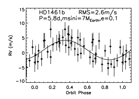
Figure 2: Phase folded radial velocity curve of HD 1461. The RV measurements are from TOU. The planet has a period of 5.8 d, and eccentricity of 0.1. The best-fit Keplerian orbital model is also shown, with a residual rms of 2.6  m s^-1 . These RV observations demonstrate TOU has the ability to detect super-Earths around nearby bright stars.

2.2 Keck/HIRES RV Data

The HIRES (Vogt et al., 1994) spectrograph covers a wavelength range of 3700-8000Å. It uses the iodine cell technique to measure radial velocities (Butler et al., 1996). Butler et al. (2017) released 20 years of precision radial velocities from HIRES on the Keck-I telescope carried out by the Lick-Carnegie Exoplanet Survey (LCES) Team. HD 26965 was one of the targets covered by this survey. We found a total of 284 observations for HD 26965 from Butler et al. (2017). We find there exists a $\sim 30$ m s^-1 offset between the RV data for HD 26965 before and after 2014 August. Such a big RV offset may be triggered by many causes, such as instrument effects, bad wavelength calibration, or data reduction pipeline glitch. Since we can not identify the exact cause for such a big RV offset, we decide to use only the 236 RV data points taken on 92 nights before 2014 August in this study to minimize inconsistency potentially caused by bad RV data products. It is worth pointing out that Díaz et al. (2018) also only use HIRES RV data taken before 2014 August in their paper. The S-indices from Ca II H and K lines derived from Keck/HIRES data are also available from (Butler et al., 2017).

2.3 HARPS RV Data

HARPS is a pressure and temperature stabilized spectrograph, which has a spectral resolving power of R$\sim$115,000 and a wavelength range between 3800 and 6300Å(Mayor et al., 2003). The HARPS data for HD 26965 are downloaded from the ESO PHASE3 archive website. We find a total of 483 good exposures on 78 nights from 2003 October to 2015 January, with exposure times ranging between 30 seconds to 10 mins, which are labeled as HARPS old data. HARPS vacuum enclosure was opened in 2015 as part of an upgrade campaign. We include 82 HARPS post-upgrade RV measurements between 2015 September and 2016 March from (Díaz et al., 2018), which are labeled as HARPS new data throughtout this paper. The spectral data are reduced using the standard HARPS Data Reduction Software (DRS).

2.4 PFS RV Data

The Carnegie Planet Finder Spectrograph (PFS) has spectral resolution of $R\sim 80,000$, and is equipped with an I₂ cell for precise radial velocity measurements. Spectroscopic observations were carried out using PFS (Crane et al., 2010) between 2011 and 2016. There are a total of 68 individual radial velocity measurements obtained on 20 different nights. The typical signal-to-noise ratio is $\sim$300 per resolution element, which delivers a level of $\sim$1-2  m s^-1 RV precision. The PFS RV measurements data and corresponding S-indices are taken from Table 8 in Díaz et al. (2018).

2.5 CHIRON RV Data

CHIRON is a fiber-fed high-resolution echelle spectrograph with a resolution of $R\sim 95,000$ using the slit mode and 3$\times$1 pixel binning (Tokovinin et al., 2013). It has a wavelength coverage of 4150 to 8800Å. The wavelength calibrated spectra are reduced using a pipeline from Brewer et al. (2014). The Doppler shifts are calculated using a standard I₂ technique. There are a total of 258 measurements taken on 107 nights, with a median radial velocity error of $\sigma=1.60$ m s^-1 . The RV measurements are taken from Table 9 in Díaz et al. (2018).

2.6 Photometric Observations

We acquired 1550 good photometric observations of HD 26965 during 24 consecutive observing seasons between 1993 September and 2017 February, all with the T4 0.75 m automatic photoelectric telescope (APT) at Fairborn Observatory in the Patagonia Mountains of southern Arizona. The T4 APT is one of several automated telescopes operated at Fairborn by Tennessee State University and is equipped with a single-channel precision photometer that uses an EMI 9924B bi-alkali photomultiplier tube to count photons in the Strömgren $b$ and $y$ pass bands (Henry et al., 1999). Further information on the operation of our automated telescopes, precision photometers, and observing and data reduction techniques can be found in Henry (1995a), Henry (1995b), Henry et al. (1999) and Eaton, Henry, & Fekel (2003).

3 Stellar Parameters

HD 26965 is the primary of a very widely separated triple system. The other two companions are an M4 dwarf and a white dwarf. The on-sky separation between the primary and the other two stars is about 82 arcsec. The estimated orbital period of this system is $\sim 8000$ years (Heintz, 1974). This star has a star spot activity cycle period of 10.1 years (Baliunas et al., 1995).

The stellar parameters are derived from excitation and ionization equilibria of Fe. We first normalize the stellar spectra in each order and merge them into a single spectrum in the spectral range 465-617 nm. We then derive equivalent widths (EWs) of Fe I and Fe II lines with the code TAME (Kang & Lee, 2012), using an initial line list with 75 Fe I and 10 Fe II lines from Tsantaki et al. (2013), after discarding Fe lines with EW $>120$ mÅ and with EW $<10$ mÅ. The stellar atmospheric parameters are computed using the code StePar (Tabernero et al., 2012), which uses the MOOG code (in its 2014 version, Sneden, 1973) and a grid of Kurucz ATLAS9 plane-parallel model atmospheres (Kurucz, 1993). StePar iterates until the slopes of A(Fe I) versus $\chi$ and A(Fe I) versus log(EW/$\lambda$) are equal to zero, while imposing the ionization equilibrium condition A(Fe I)$=$A(Fe II). StePar does a second iteration of the stellar parameter determination after rejecting the Fe lines with an EW and corresponding Fe abundance outliers using a 3-$\sigma$ clipping procedure. 61 Fe I lines and 9 Fe II lines remain after clipping, which produce $T_{\rm eff}=5072\pm 53$ K, $\log(g)=4.45\pm 0.19$, [Fe/H]$=-0.42\pm 0.04$. Therefore, HD 26965 is a metal poor star compared to our Sun. Using the mass-radius-stellar parameters relation from Torres, Andersen, & Giménez (2010), we calculate HD 26965 to have a stellar mass of 0.78$M_{\odot}$ and a stellar radius of 0.87$R_{\odot}$. We listed these parameters in Table 2.

For comparison, the stellar parameters for HD 26965 were also derived from HARPS spectra by Delgado Mena et al. (2017). The abundances were determined from a standard local thermodynamic equilibrium (LTE) analysis using measured equivalent widths (EWs) injected into the code MOOG and a grid of Kurucz ATLAS9 atmospheres. They reported $T_{eff}=5098\pm 32$ K, $\log(g)=4.35\pm 0.10$, [Fe/H]$=-0.36\pm 0.02$, which are consistent with our results from our TOU spectra. Díaz et al. (2018) also derived stellar parameters for HD 26965, which agree with our results as well. Therefore, we only report our results from TOU in Table 2.

We also did a SED fitting using Johnson UBV (Ducati, 2002), Stromgren uvby, and JHK (Cutri et al., 2003) band photometry, which is shown in Figure 3. Using the PARSEC database of stellar evolutionary tracks (Bressan et al., 2012), we found the star has a stellar age of 6.9$\pm 4.7$ Gyr. The error bar is big because K0 dwarfs usually stay on their main sequence for up to 15 Gyr.

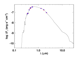
Figure 3: The observed SED from the optical through the IR for HD 26965, along with Kurucz ATLAS model atmosphere. Blue points represent the expected fluxes in each band based on the model, red horizontal bars are the approximate bandpass widths, and red vertical bars are the flux uncertainties.

Table 2: Stellar Parameters of HD 26965

Parameter	Value
Effective Temperature	5072$\pm 53$ K
log(g)	4.45$\pm 0.19$
$\rm[Fe/H]$	$-0.42\pm 0.04$
Spectral Type	K0 V
Mass (Torres)	0.78 $\pm$ 0.08 $M_{\odot}$
Radius (Torres)	$0.87\pm 0.17R_{\odot}$
Radius (SED)	$0.812\pm 0.017R_{\odot}$
$\rm log(R^{{}^{\prime}}_{HK})$	$-4.99^{a}$
Age	6.9$\pm$4.7 Gyr
$A_{V}$	$0.00^{+0.01}_{-0.00}$
$F_{\rm bol}$	$5.06\pm 0.12$e-7 erg/s/cm2
Distance from Hipparcos	$4.985\pm 0.001$ pc
aData from Jenkins et al. (2011).

4 MCMC Fitting of RV Data

In order to quantify the uncertainties of the orbital parameters of the planet, we perform an MCMC analysis using the python code emcee. Our code follows the Bayesian method described in Gregory (2005) and Ford (2005, 2006). Any noise component that cannot be modeled is described by a stellar jitter term $\sigma_{jitter}$ for each corresponding instrument.

Each state in the Markov chain is described by the parameter set

$$\vec{\theta}=\{P_{b},K_{b},e_{b},\omega_{b},M_{1},C_{i},\sigma_{\rm jitter}\},$$ (1)

where $P_{b}$ is orbital periods, $K_{b}$ is the radial velocity semi-amplitudes, $e_{b}$ is the orbital eccentricities, $\omega_{b}$ is the arguments of periastron, $M_{b}$ is the mean anomalies at chosen epoch ($\tau$), $C_{i}$ is constant velocity offset between the differential RV data from TOU, Keck, PFS, CHIRON, and HARPS and the zero-point of the Keplerian RV model, and $\sigma_{\rm jitter}$ is the “jitter” parameter. The jitter parameter describes any excess noise, including both astrophysical noise (e.g. stellar oscillation and stellar spots; Wright, 2005), any instrument noise not accounted for in the quoted measurement uncertainties, and systematic RV errors.

We use standard priors for each parameter (Gregory, 2007). The prior is uniform in the logarithm of the orbital period ($P_{b}$) from 1 to 1000 days. For $K_{b}$ and $\sigma_{\rm jitter}$ we use a modified Jefferys prior which takes the form of $p(x)=(x+x_{o})^{-1}[\log(1+x_{max}/x_{o}]^{-1}$ , where $x_{o}=0.1$ ${\rm m\,s^{-1}}$ and $x_{\mathrm{m}ax}=20$ ${\rm m\,s^{-1}}$ (Gregory, 2005). Prior for $e_{b}$ is uniform between zero and unity. Priors for $\omega_{b}$ and $M_{b}$ are uniform between zero and $2\pi$. For $C_{i}$, the prior is uniform between min($v_{i}$)-50 m s^-1 and max($v_{i}$)+50 m s^-1 , where $v_{i}$ are the set of radial velocities obtained from each of the RV instruments. We verified that the chains did not approach the limiting values of $P_{b}$, $K_{b}$, and $\sigma_{\rm jitter}$.

Following Ford (2006), we adopt a likelihood (i.e., conditional probability of making the specified measurements given a particular set of model parameters) of

$$p(v|\vec{\theta},M)\propto\prod_{k}\frac{\exp[-(v_{k,\theta}-v_{k})^{2}/2(\sigma^{2}_{k,obs}+\sigma^{2}_{\rm jitter})]}{\sqrt{{\sigma_{k,obs}}^{2}+{\sigma_{\rm jitter}}^{2}}},$$ (2)

where $v_{k}$ is the observed radial velocity at time $t_{k}$, $v_{k,\theta}$ is the model velocity at time $t_{k}$ given the model parameters $\vec{\theta}$, and $\sigma_{k,obs}$ is the measurement uncertainty for the radial velocity observation at time $t_{k}$.

In Table 3 we show the final parameters and uncertainties obtained with our MCMC analysis. We performed a simultaneous fit of the planetary signal and the activity induced RV jitters using the TOU, Keck, PFS, CHIRON, and HARPS data. From the periodogram of the RV data shown in Figure 4, we find a strong periodic signal around 42-day. The $0.1\%$ significance level shown on this plot is determined after 10000 bootstrap resampling. In Figure 5 we show the best Keplerian orbital fit to the RV data which is attributed to the planet candidate HD 26965b. The phase-folded RV curve is shown in Figure 6. The RMS of the residuals is 2.6 m s^-1 , and we did not find any additional peak with significance above $0.1\%$ from the periodogram of RV residuals. Adopting a stellar mass of 0.78$M_{\odot}$, we derived the minimum mass of the planet $m\sin i=9.7\pm 1.3M_{\earth}$.

Figure 4: Generalized Lomb-Scargle periodogram for the RV data, which clearly shows the peak around 42 day. The horizontal dashed line shows the 0.1$\%$ significance level determined using 10000 bootstrap resamplings and a search window of [2, 200] days.

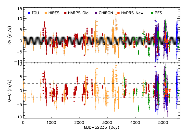
Figure 5: Best-fit 1-planet Keplerian orbital model for HD 26965. The RV data points from Keck/HIRES, HAPRS, PFS, CHIRON, and TOU are shown as yellow, red, and blue dots. The black solid line is the maximum likelihood model, with the orbital parameters listed in Table 3. The bottom panel shows the RV residuals after subtracting the best-fit Keplerian RV model. The horizontal dashed liens show the range of the rms value, $\pm 2.6$  m s^-1 .

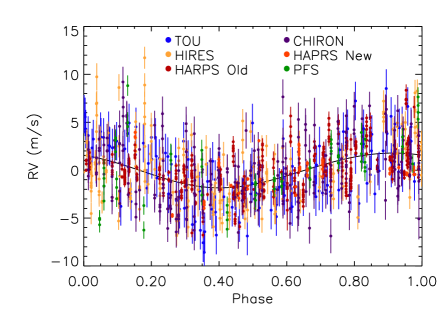
Figure 6: Phase-folded RV curve of HD 26965. The black solid line is best-fit 1-planet Keplerian orbital model, with the orbital parameters listed in Table 3.

Table 3: MCMC Posteriors for the Keplerian Orbital Fitting

Parameter	Credible Interval	Maximum Likelihood	Units
$P_{b}$	42.378 $\pm 0.01$	42.378	days
$T\rm{conj}_{b}$	5886.76 ${}^{+0.62}_{-0.58}$	5886.50	JD
$e_{b}$	0.04${}^{+0.05}_{-0.03}$	0.02
$\omega_{b}$	2.6 ${}^{+2.2}_{-1.4}$	2.2	radians
$K_{b}$	1.81 ${}^{+0.10}_{-0.10}$	1.80	m s-1
$C_{\rm TOU}$	-0.32 $\pm 0.26$	-0.31	m s-1
$C_{\rm HIRES}$	0.23 $\pm 0.23$	0.24	m s-1
$C_{\rm PFS}$	-0.37 $\pm 0.39$	-0.38	m s-1
$C_{\rm CHIRON}$	0.16 $\pm 0.19$	0.16	m s-1
$C_{\rm HARPS_{o}ld}$	0.05 $\pm 0.09$	0.0.04	m s-1
$C_{\rm HARPS_{n}ew}$	-0.02 $\pm 0.23$	-0.02	m s-1
$\sigma_{\rm TOU}$	2.06 ${}^{+0.28}_{-0.27}$	2.03	$\rm m\ s^{-1}$
$\sigma_{\rm HIRES}$	3.08 ${}^{+0.19}_{-0.17}$	3.06	$\rm m\ s^{-1}$
$\sigma_{\rm PFS}$	2.82 ${}^{+0.32}_{-0.28}$	2.70	$\rm m\ s^{-1}$
$\sigma_{\rm CHIRON}$	2.41 ${}^{+0.18}_{-0.16}$	2.39	$\rm m\ s^{-1}$
$\sigma_{\rm HARPS_{o}ld}$	1.81 ${}^{+0.07}_{-0.6}$	1.80	$\rm m\ s^{-1}$
$\sigma_{\rm HARPS_{n}ew}$	1.91 ${}^{+0.19}_{-0.15}$	1.88	$\rm m\ s^{-1}$
$m\sin i$	8.47$\pm 0.47$	8.43	$M_{\earth}$

5 Planet, or Stellar Activity?

In this section, we discuss the possibility that the RV signal is actually produced by stellar rotation modulated activity (like starspots, plagues, and convection inhibition; Dumusque et al., 2011). We first determine the possible stellar rotation periods from both stellar activity index and photometric data, and compare them with the period of the RV signal. We then assess the stability of this 42-day RV signal by investigating the evolution of this 42-day RV signal against the number of RV observations. We also discuss the possible RV jitter induced by stellar surface activity and compare it with the amplitude of the 42-day RV signal. Line bisector analysis is conducted in the end to investigate the impact of stellar activity on RV measurements. All of the studies except the activity period in this section support the planet origin of the 42-day RV signal, which are summarized in Table 4.

Table 4: Summary of evidence supporting planet origin or stellar activity origin of the detected 42 d RV signal.

Evidence	Planet or Activity Origin
$P_{\rm rotation}$ close to 42 d	Activity
Sharp 42 d peak from RV periodogram	Planet
No clear 42 d peak from $S_{\rm MW}$ periodogram	Planet
Clear 42 d peak from magnetic quiet phase RV periodogram	Planet
Clear 42 d peak from magnetic active phase RV periodogram	Planet
Strong 39 d signal from $S_{\rm MW}$ in magnetic quiet phase	Planet
Strong 41 d signal from $S_{\rm MW}$ in magnetic active phase	Planet
No 42 d peak from 23 years high precision photometric campaign	Planet
Star spots $K_{\rm spot}<0.3$ m s-1 from simulation	Planet
Inhibition of convection $K_{\rm inh}<0.3$ m s-1 from linear interpolation	Planet
Active phase and quiet phase have similar $K$ values detected	Planet
No strong correlation between RV and BIS	Planet

5.1 Stellar Activity Index and Rotation Period

We first determine the rotation period of the star using the stellar activity S index. The S index, calculated from the singly ionized calcium H & K line core emission flux (Wilson, 1978), is the most commonly used index of stellar magnetic activity. To put constraints on the rotation period and the magnetic activity cycle of the star, we re-examined the Ca II HK S index data from Mount Wilson ($S_{\rm MW}$), HARPS, Keck, and PFS. Olin Wilson’s HK Project at the Mount Wilson Observatory (MWO) regularly observed the Ca II HK emission for a sample of over 100 bright dwarf stars beginning in 1966 to characterize magnetic variability of stars other than the Sun (Wilson, 1978). We obtained the Mount Wilson data from the National Solar Observatory (NSO) and present them in Figure 7. From the plot, we can clearly see a 10.1 yr magnetic cycle (also reported in Baliunas, Sokoloff, & Soon, 1996), which shows the star periodically enters into an active phase after a relatively quiet phase. Since there is a $\sim 10$ yr magnetic cycle, we need to remove its signal first before we can examine the short-term $S_{\rm MW}$ variations caused by stellar rotation. We used a spline function with a breakpoint of 200 days to de-trend the $S_{\rm MW}$ values. For the S index data from HAPRS, KECK, and PFS, we use a breakpoint of 500 days because there are not as many data points available as there are from Mount Wilson. After examining the periodogram for the de-trended $S_{\rm MW}$, we do not find a clear peak at 42.4 d. From the study of the Sun, we learn that the active regions are not always concentrated on certain longitudes, hindering the detection of its stellar rotation signal during the active phase. Therefore, we decide to separate these S index data alternatively into the quiet phase and active phase as shown in zone 1 to 9 in Figure 7 to check for occasionally strong periodic signals.

The periodogram for these marked zones are shown in Figure 8. We found strong signals in zone 5 and zone 6, corresponding to an active phase and a quiet phase, respectively. Since the S index data from HAPRS, KECK, and PFS do not have error bars, we decided to not run periodograms and Sine curve fitting on these data. The S index data from Zone 5 and Zone 6 together with their best Sine curve fit are displayed in Figure 9. HAPRS, Keck, and PFS S index data from Zone 8 and 9 are also displayed in Figure 9, which support consistent periodic signals found from the Mount Wilson data in both the active and quiet phases. The resulting best-fit periods for the active and quiet phases are $41.2\pm 0.9$ days and $39.2\pm 0.7$ days, respectively, with errors estimated from the FWHMs of the peaks in the periodograms. The period variation can be explained by the differential rotation of the star and different locations of active regions similar to our Sun. For comparison, the periodograms of radial velocities in both the active phase and quiet phase (Figure 10) clearly show a stable peak around 42.4 d. The fact that periodograms for the activity indicator $S_{\rm MW}$ show multi-peaks, and none of these strong peaks sit exactly at 42.4 d, is an important piece of evidence supporting the planet origin of this 42.4 d signal. The best-fit amplitudes of the S index modulation (Figure 9) are 0.008 and 0.017 in the quiet phase and the active phase, which demonstrates there is stronger stellar surface activity during the magnetic active phase than during the quiet phase. As explained later in section 5.4, this finding also supports the planet origin of this 42.4 d signal.

There are several other estimates of the stellar rotation period from previous work, like 43 days using 25 years of the Ca II HK index measurements from Mount Wilson Observatory (Baliunas, Sokoloff, & Soon, 1996), 42.2 days using the calibrated stellar activity-rotation-age relation (Mamajek & Hillenbrand, 2008; Lovis et al., 2011), 43.7 days using the relation from (Suárez Mascareño et al., 2015; Suárez Mascareño, Rebolo, & González Hernández, 2016). All of the rotation periods estimated above, including our own result, are close to the period of the RV signal detected in this paper, which warrants further discussion of the possibility that this RV signal is induced by stellar surface magnetic activity.

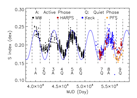
Figure 7: Measurements of Ca II HK S index of HD 26965. The data are collected from Mount Wilson observatory (black), HARPS (red), Keck (blue), and PFS (orange). We over-plotted a Sine curve with a 10.1 yr period to show the sun-like magnetic cycle. The data are separated into alternative magnetic quiet and active phases, which are marked by a zone number from 1 to 9. In the plot, ‘A’ represents magnetic active phase, and ‘Q’ represents magnetic quiet phase.

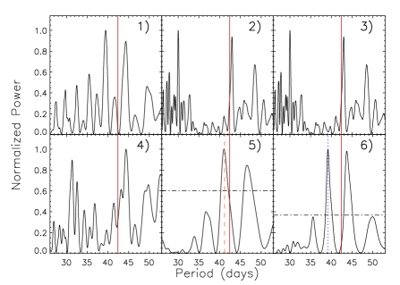
Figure 8: Periodograms for the Mount Wilson Ca II HK S index. From top left to bottom right, the panels show periodograms of $S_{\rm MW}$ from zone 1 to zone 6 marked as in Figure 7. We searched for strong periodic signals around 42 days in each zone. The horizontal dashed lines shown in panel 5 and 6 mark the $0.1\%$ significance level, which is derived using 10000 times bootstrap resampling and a search window of [2, 300] days. The red vertical solid line in each panel shows the period of the planet candidate HD 26965b at 42.4 d. The orange vertical dashed line in panel 5 shows the period of a strong signal in a magnetic active phase at 41.2d. The blue dotted vertical line in panel 6 shows the period of the strong signal in a magnetic quiet phase at 39.2d.

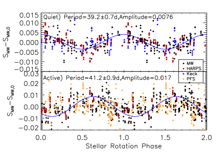
Figure 9: Phase folded Mount Wilson, HAPRS, Keck, and PFS S index measurements of HD 26965. The data shown in the top panel are from the magnetic quiet phase, and the data in the bottom panel are from the magnetic active phase. We fitted a Sine function to the S index after subtracting their median value, and calculated the best-fit period and amplitude for both phases using the Mount Wilson data. The S indices from HARPS, Keck, and PFS were not used in the Sine curve fitting, but they are consistent with the rotation period fitted from the Mount Wilson data. The active phase shows a bigger S index variation amplitude due to a more active status of the star compared to the quiet phase.

Figure 10: Periodograms for the radial velocities for alternating active (the top panel) and quiet phases (the bottom panel), respectively. Both periodograms show a clear peak around 42.4 d, which is marked with a vertical red solid line. The horizontal dashed line in each panel marks the $1\%$ significance level, which is derived using a 1000 times bootstrap resampling and a search window of [2, 300] days.

5.2 Photometric Results and Rotation Period

Figure 11: Photometric data of HD 26965 acquired with the T4 APT at Fairborn Observatory from 1993 to 2017. A total of 1550 differential photometric data points of HD 26965 are phased to the period of the planet RV signal. The two horizontal dashed line correspond to the $\pm 1\sigma$ range of the brightness level of the 1550 observations.

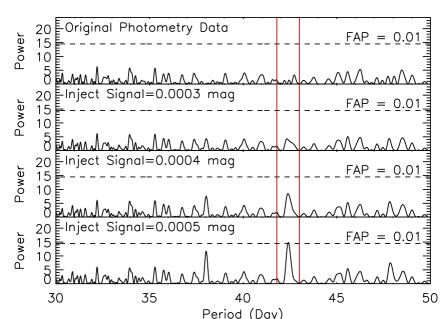
Figure 12: Periodogram of photometric data for HD 26965 from Fairborn. There is no significant peak except the 1-day alias in the top panel. The double red solid lines mark the region around $P=42.38$ d, which is the planet orbital period. In the second, third and fourth panels, we inject a periodic signal at semi-amplitudes of 0.0003, 0.0004, and 0.0005 mag to the original photometric data. The peak at 42 days becomes higher as the injected signal becomes stronger. Comparing the simulated periodogram with the original periodogram in the top panel, we can rule out a periodic signal stronger than $0.0004$ mag. We note here that the 1 year alias of the 42.4 d signal, which sits at 38 d, also becomes stronger.

In this section we search for a periodic rotation signal from photometric data. In Figure 11 we plot all 1550 photometric measurements from Fairborn Observatory plotted against the orbital phase of HD 26965b with $P_{b}=42.38$ d. The standard deviation of these data from their mean is 0.002 mag. A least-squares Sine-curve fit to the phased data gives a full amplitude of $0.0000\pm 0.0002$ mag. We can rule out a sinusoidal brightness variation larger than 0.0006 mag at 3-$\sigma$ confidence at the orbital period of the planet candidate. To put further constraint on the upper limit of a detectable periodic photometric signal that might be induced by starspots, we did a simple simulation by adding a sinusoidal photometric signal to the photometric data collected from Fairborn. The period for this signal is set to be the same as the period of the planet signal ($P=42.38$ d), and the semi-amplitude is chosen to be $0.0003$, $0.0004$, and $0.0005$ mag. From the periodogram shown in Figure 12, we cannot detect the $0.0002$ mag signal, but can start to detect this periodic photometric signal at $0.0005$ mag. This simulation helps rule out a detectable periodic photometric signal with a semi-amplitude larger than 0.0004 mag. We use this information to put a constraint on stellar RV jitters induced by starspot activity in the next section.

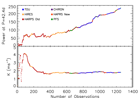
Figure 13: Evolution of the significance of the detected signal and its semi-amplitude as a function of the number of measurements. The semi-amplitude is derived using a fixed orbital period and eccentricity.

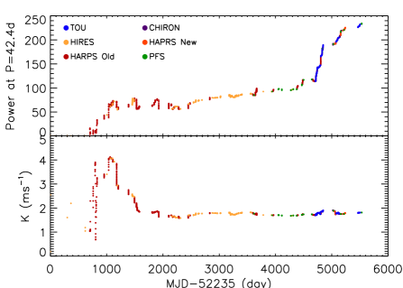
Figure 14: Evolution of the significance of the detected signal and its semi-amplitude as a function of the date of the observations. The semi-amplitude is derived using a fixed orbital period and eccentricity.

5.3 RV Signal Evolution

To assess the stability of this RV signal, we study the evolution of this 42-day RV signal against the number of observations and date of observations in this section. The significance power of this 42-day signal is calculated using a generalized Lomb-Scargle periodogram (GLS) following Zechmeister & Kürster (2009). Figure 13 shows the evolution of the signal significance and its velocity semi-amplitude ($K$) against number of observations. The evolution of this 42-day signal is steady and continuous after $N=400$ data points. Figure 14 shows the evolution of the signal significance and its velocity semi-amplitude ($K$) against the date of observation. By studying the evolution against the date of observations, we can also see the importance of the high-cadence Dharma survey observations. The slope of the significance increased after the start of the TOU nightly cadence campaigns in 2015, which means that the time needed for the detection of short-period planets decreases significantly, similar to what happened with the discovery of Proxima b (Anglada-Escudé et al., 2016). If this 42-day RV signal is generated by stellar activity, it should not be so stable given the large amplitude variation of stellar activity strength from its magnetic cycle. These two plots support the stableness of the orbital parameters and, thus, the planetary source of this 42-day RV signal (Suárez Mascareño et al., 2017a).

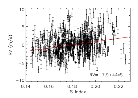
Figure 15: Correlation between Ca II HK S index and radial velocity measured by HARPS, HIRES, and PFS. The red solid line shows the best linear-fitting result ($RV=-7.9+44\times S$).

5.4 Stellar Activity RV Jitter

In this section, we provide additional evidence to support the planet nature of this RV signal. There are several stellar activity sources that can generate an RV signal detected in this paper, like dark spots, plages, and convection inhibition (Vanderburg et al., 2016). We discuss these possibilities in this section. First, we simulated the RV signal induced by dark spots using a modified code of SOAP2.0 (Spot Oscillation And Planet, Dumusque, Boisse, & Santos 2014; Kimock et al., in preparation). By setting a photometric variation semi-amplitude of $0.0004$ mag, the upper limit derived from the last section, and using a single spot model for simplicity, the maximum RV signal generated has $K_{\rm spot}<0.3$  m s^-1 , which is a factor of seven times less than the RV signal detected. We also explored a more realistic multi-spot model similar to the Sun in our simulation; the RV signal generated is even smaller in the $K_{\rm spot}$ value, similar to what was concluded in the previous study by Dumusque, Boisse, & Santos (2014).

Secondly, the inhibition of convection due to surface magnetic activity can generate artificial redshift. Solar-like magnetic cycles are characterized by an increasing filling factor of active regions when the activity level increases. Because convection is strongly reduced in active regions as a result of the magnetic field, the star appears redder (thus positive radial velocity) during its high-activity phase. A positive correlation between the RVs and the activity level is therefore observed (Meunier, Lagrange, & Desort, 2010). However, neither Santos et al. (2010) nor Lovis et al. (2011) found any significant RV variation from HD 26965 due to convection inhibition during its magnetic cycle ($<2$ m s^-1 ). Here we reproduced this correlation in Figure 15 using the RV and Ca II HK S-indices data from HARPS, PFS, and Keck/HIRES, and made a linear fit to this correlation. We came to the same conclusion as stated by Santos et al. (2010), that there is a very weak correlation between the RV and Ca II HK S-index. Using the linear relation from Figure 15, the convection inhibition can generate an RV variation with a semi-amplitude $K_{\rm inh}\sim 0.2$ m s^-1 within a 42 day period when the periodic coherent Ca II HK S-index variation is as small as $\sim$0.004 (semi-amplitude) shown in the top panel of Figure 9. Clearly this is not big enough to explain the semi-amplitude of $\sim$1.8 m s^-1 RV signal detected.

The above discussions show that the most common types of magnetic activity cannot induce the RV signal detected in this investigation. Next we present additional evidence against the activity origin of this 42-day RV signal. In the previous section, we identified the magnetic active phases and quiet phases based on over 30 years of Ca II HK index measurements of HD 26965 (Figure 7). We then divided all the RV measurements into either an active phase or a quiet phase. The phased curves of Ca II HK index measurements in Figure 9 show that the surface activity filling factor varies a factor of two between the quiet phase and the active phase. Lanza et al. (2016) found there is a positive correlation between solar RV variation and the level of chromospheric activity measured using Ca II HK index. If the coherent 42-day RV signal detected is from stellar activity modulated by the rotation, we expect the RV amplitude would become two times larger in the active phase than in the quiet phase because the coherent S-index variation in the active phase is twice as large as that in the quiet phase. Since HARPS RV data span over more than 10 years, we choose to use HARPS RV data to test this scenario. After dividing HAPRS RV data into active phase and quiet phase data, we did a Keplerian RV fitting for each phase. During the fitting, we fixed two parameters with $P=42.38$ day and $e=0.0$ to focus on the velocity semi-amplitude variation. The fitting results are shown in Figure 16, with $K_{\rm active}=1.7\pm 0.3$ m s^-1 and $K_{\rm quiet}=1.8\pm 0.4$ m s^-1 . The fact that RV amplitude does not increase significantly from the quiet phase to the active phase again supports the planet origin of this 42-day RV signal.

In Suárez Mascareño et al. (2017b), they studied the radial velocity signal induced by stellar activity and rotation among 55 late-type dwarf stars using HARPS data. They derived an empirical relationship between the mean level of chromospheric emission and the radial velocity semi-amplitude shown in Figure 9 of their paper. Using $\rm log(R^{{}^{\prime}}_{HK})=-4.99$ from Jenkins et al. (2011), we estimate that the expected RV signal at this level of stellar activity is $\sim$0.35 m s^-1 , which is much smaller than the stable $\sim$1.8 m s^-1 RV signal detected. This also supports the planet origin of this 42-day RV signal.

Vanderburg et al. (2016) conducted extensive sets of simulations to study the impact of stellar surface activity modulated by stellar rotation on the ability to detect planets using the radial velocity technique. In their simulations, they usually assume RV observations with ideal sampling, which is similar to the situation in this paper when combining the Keck/HIRES, HARPS, PFS, CHIRON, and TOU observations. They found that an activity signal identified from the RV periodogram at a period of $P_{\rm activity}$ usually has a width as large as $\sim 0.1*P_{\rm activity}$ because of the lifetime of spots and differential stellar rotation. While in our RV periodogram, the peak at 42 day is very sharp with a $FWHM=0.3$ d. This points to the likely conclusion that the coherent 42-d RV signal found from HD 26965 is induced by a planet, not magnetic activity.

5.5 Line Bisector Analysis

Line bisector analysis is another diagnostic tool to investigate the possible impact of stellar activity on RV measurements (Toner & Gray, 1988; Queloz et al., 2001; Wright et al., 2013). Here we performed a correlation study of the Bisector Inverse Slope (BIS) and the radial velocities from the fiber-fed TOU spectrograph. In our RV data pipeline, we do not use the Cross-Correlation Function (CCF) method employed by HARPS (Ma & Ge, in preparation). Instead we use a template matching method similar to Zechmeister et al. (2018). Thus, we do not have a traditional CCF product from our pipeline to calculate the BIS. Instead, we used the reduced-$\chi^{2}$ function from our template matching pipeline to calculate the BIS. Similar to the method employed by Santos et al. (2002) on their analysis of the HARPS CCF, we compute the bisector velocity for 10 different levels on the reduced-$\chi^{2}$ function from TOU. The Bisector Inverse Slope is calculated by averaging the upper and lower bisector points before subtracting one from the other. Here we choose the definition from (Queloz et al., 2001) where they use the 10-40$\%$ and 55-85$\%$ CCF depth (see also Wright et al., 2013). This quantity is equivalent to the BIS from the CCF method since both trace the asymmetry in the absorption line profile variation caused by stellar surface activity. The Spearman’s rank correlation coefficient between the RV and the BIS is 0.15 with a significance level of 0.08, which suggests there does not exist a strong correlation between the RV and BIS. This is more strong evidence to argue against the activity origin of the 42-day RV signal.

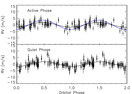
Figure 16: Radial Velocity data from HARPS, which are divided into quiet (bottom panel) and active (top panel) phases according to the magnetic cycle of the star. We use $P=42.38$ d and $e=0$ to fit the RV data to study the RV amplitude variation from the quiet phase to active phase. The black lines in both panels show the best-fit RV models, and the blue solid line in the top panel shows a model with an RV amplitude two times of that from the quiet phase. The fitting result does not support the hypothesis that the RV amplitude in the active phase became twice as large as that in the quiet phase, which supports the planet origin of the 42-day RV signal.

6 Conclusion and Discussion

In a search through the early RV data from the DPS survey, we discovered an RV signal consistent with a super-Earth orbiting a V=4.4 K dwarf, HD 26965. Additional RV data were found from the Keck archive and HARPS archive. After combining the RV data from the DPS survey with data from Keck/HIRES and HAPRS, we use an MCMC code to find the best-fit orbital parameters with an orbital period of 42.38$\pm 0.01$ d, eccentricity of 0.04${}^{+0.05}_{-0.03}$, and velocity semi-amplitude of $1.81\pm 0.10$ m s^-1 . Adopting a stellar mass of 0.78$M_{\odot}$ for HD 26965, the minimum mass for the planet is 8.47$\pm 0.47$ Earth masses, which puts it in the super-Earth mass range.

The 42-day period RV signal has also been reported in Díaz et al. (2018). We privately communicated about our discoveries during the 2017 summer Extremely Precise RV meeting (EPRV) at the Pennsylvania State University. The best Keplerian solution reported from their modeling has a $P=42.364\pm 0.015$ d, $e=0.017\pm 0.046$, and $K=1.59\pm 0.15$ m s^-1 . The periods reported from our paper and their paper are similar. The fact they reported a smaller RV signal may be related to their modeling of red noise and linear correlations with stellar activity indicators, in addition to the white noise used in our RV modeling.

The conclusion from Díaz et al. (2018) is that the RV signal can be either from a planet or from stellar activity. Using Ca II HK index variation, we find this star does show a long-term magnetic cycle of $\sim 10.1$ yr. The fact that the orbital period of the planet is close to the rotation period of the star is concerning, because stellar rotation modulation of magnetic activity can mimic planet signals (Saar & Donahue, 1997; Desort et al., 2007; Ma & Ge, 2012). For instance, Queloz et al. (2001) found that the RV variation of a G0V star, HD 166435, is from surface spot activity, not a planet. Huélamo et al. (2008) and Huerta et al. (2008) also found that two previously claimed exoplanets are actually caused by starspots on the stellar surface. Mahmud et al. (2011) showed that cool surface spots could cause the periodic RV variability on a T Tauri star.

By carefully examining the RV data in the active phase and quiet phase of the star, and after carefully considering all possible stellar activity sources, we concluded that the coherent signal seen from HD 26965 is most likely from a planet, with some RV noise contributed by stellar activity. In addition, the sharpness of the 42 day peak in the RV periodogram also supports the planet origin of the 42-d RV signal as active regions on the stellar surface modulated by differential rotation of the star normally reveal themselves as a group of peaks around the mean rotation period (Vanderburg et al., 2016). The evolution of the RV semi-amplitude to a stable value after several years of observations provides additional strong support for the planet origin of this 42-day RV signal. Our high quality photometric dataset helps rule out any significant photometric variation at 42 days. This also supports the planet origin of this 42-day RV signal. This plethora of evidence allows us to draw the conclusion that this 42-day RV signal is from a planet, unlike the uncertainties reported in Díaz et al. (2018).

Currently there are several planet systems known to host planets with periods close to the rotation period of the star (Dragomir et al., 2012; Haywood et al., 2014), or close to the magnetic cycle period of the star (Wright et al., 2008; Kane et al., 2016). For example, Dragomir et al. (2012) found a Jupiter-mass planet orbiting HD 192263 with a period of 24.4 days using radial velocity from Keck/HIRES and CORALIE, and derived a stellar rotation period of 23.4 days using photometric data. We note here that Henry et al. (2002) initially suggested that the RV signal around HD 192263 is caused by rotational modulation of surface activity. But Santos et al. (2003) used significant changes of photometric patterns over time and 3 years of coherent RV observations to prove that the signal is indeed from a planet. In the case of HD 26965, we cannot derive a precise stellar rotation period because our ground-based photometric data did not reveal any significant periodic variation around 42 days. Future high precision space photometric observations can help detect possible small photometric variation from the star ($<400$ ppm) caused by the surface spots. As pointed out by Vanderburg et al. (2016), it is very important for next generation RV planet surveys to have simultaneous photometric observations for measuring rotation periods and activity signals. Our data analysis also demonstrates the importance of having simultaneous photometry for the purpose of disentangling planet signals from magnetic activity signals.

HD 26965 is a very bright metal poor star with V=4.4. This makes it the second brightest star in the night sky with a super-Earth detection so far, just behind HD 20794 (V=4.3 Pepe et al., 2011). One interesting fact is that HD 20794 has a similar metallically (Fe/H$=-0.4\pm 0.1$) as that of HD 26965 (Fe/H$=-0.42\pm 0.04$), which is consistent with the finding of Petigura et al. (2018) that smaller planets are detected around stars with wide-ranging metallicities.

Based on the observed properties of HD 26965 b, several inferences of the planet’s properties and history are possible. With a minimum mass of 8.4$M_{\earth}$, the planet likely possesses a gaseous atmosphere based on other planets with known masses and radii (Rogers, 2015). However, we note that Kepler-10 c has a similar mass and orbit, is hosted by a similar, low-metallicity star (Batalha et al., 2011; Fressin et al., 2011; Weiss et al., 2016; Rajpaul, Buchhave & Aigrain, 2017), and does not possess an envelope (Lopez & Fortney, 2014), so HD 26965 b may be a similar type of world. In the near-term, this possibility can only be resolved if a transit is detected.

Figure 17: Phased photometric data of HD 26965 from Fairborn Observatory. It is an expanded version of Figure. 11. This figure is centered on the predicted middle transit time. The solid curve shows the predicted central transit signal with a depth of 0.0008 mag. The current data do not support the existence of a transit signal.

Detecting exoplanets via the RV technique and subsequently monitoring their transit windows is one of the most fruitful strategies for finding bright stars with transiting planets, which are the best candidates for exoplanet atmospheric studies. Figure 17 shows the photometric data near the predicted middle transit time. The expected duration of a central transit is $\sim$$R_{\star}P/(\pi a)=5.8$ hr, and the expected depth is $(R_{b}/R_{\star})^{2}$$\sim$0.0008. Our current photometric data do not support the existence of a shallow transit from HD 26965b.

Lastly, the detection of HD 26965b shows the advantage of the Dharma planet survey strategy. The high precision and high cadence RV campaign from TOU have greatly increased the detection sensitivity of low-mass planets. The fact that we can discover this system with similar RV precision to HAPRS (Ma & Ge, in preparation), but with high cadence (133 nights observations within 2 years using TOU versus 97 nights observations within 13 years using HARPS), demonstrates that high precision and high cadence RV surveys of bright stars in the solar neighborhood will likely lead to the detection of a large number of low-mass planets with high completeness, and possible detections of low-mass planets in their habitable zones (Ge et al., 2016).

References

- Aurière (1982) Aurière, M. 1982, A&A, 109, 301
- Anglada-Escudé et al. (2016) Anglada-Escudé G., et al., 2016, Natur, 536, 437
- Baliunas et al. (1995) Baliunas S. L., et al., 1995, ApJ, 438, 269
- Baliunas, Sokoloff, & Soon (1996) Baliunas S., Sokoloff D., Soon W., 1996, ApJ, 457, L99
- Batalha et al. (2011) Batalha N. M., et al., 2011, ApJ, 729, 27
- Batalha et al. (2013) Batalha N. M., et al., 2013, ApJS, 204, 24
- Barnes et al. (2016) Barnes R., et al., 2016, arXiv, arXiv:1608.06919
- Bonfils et al. (2013) Bonfils X., et al., 2013, A&A, 549, A109
- Borgniet et al. (2017) Borgniet S., Lagrange A.-M., Meunier N., Galland F., 2017, A&A, 599, A57
- Bressan et al. (2012) Bressan A., Marigo P., Girardi L., Salasnich B., Dal Cero C., Rubele S., Nanni A., 2012, MNRAS, 427, 127
- Brewer et al. (2014) Brewer, J. M., Giguere, M., & Fischer, D. A. 2014, PASP, 126, 48
- Buchhave et al. (2016) Buchhave L. A., et al., 2016, AJ, 152, 160
- Burke et al. (2015) Burke C. J., et al., 2015, ApJ, 809, 8
- Butler et al. (1996) Butler, R. P., Marcy, G. W., Williams, E., et al. 1996, PASP, 108, 500
- Butler et al. (2017) Butler R. P., et al., 2017, AJ, 153, 208
- Christiansen et al. (2016) Christiansen J. L., et al., 2016, ApJ, 828, 99
- Coughlin et al. (2016) Coughlin J. L., et al., 2016, ApJS, 224, 12
- Crane et al. (2010) Crane, J. D., Shectman, S. A., Butler, R. P., et al. 2010, Proc. SPIE, 7735, 773553
- Cutri et al. (2003) Cutri R. M., et al., 2003, yCat, 2246,
- Díaz et al. (2018) Díaz M. R., et al., 2018, AJ, 155, 126
- Delgado Mena et al. (2017) Delgado Mena, E., Tsantaki, M., Adibekyan, V. Z., et al. 2017, A&A, 606, A94
- Desort et al. (2007) Desort, M., Lagrange, A.-M., Galland, F., Udry, S., & Mayor, M. 2007, A&A, 473, 983
- Dragomir et al. (2012) Dragomir D., et al., 2012, ApJ, 754, 37
- Dressing & Charbonneau (2015) Dressing C. D., Charbonneau D., 2015, ApJ, 807, 45
- Ducati (2002) Ducati J. R., 2002, yCat, 2237,
- Dumusque et al. (2011) Dumusque X., Udry S., Lovis C., Santos N. C., Monteiro M. J. P. F. G., 2011, A&A, 525, A140
- Dumusque et al. (2012) Dumusque X., et al., 2012, Natur, 491, 207
- Dumusque, Boisse, & Santos (2014) Dumusque X., Boisse I., Santos N. C., 2014, ApJ, 796, 132
- Eaton, Henry, & Fekel (2003) Eaton, J. A., Henry, G. W., & Fekel, F. C. 2003, in The Future of Small Telescopes in the New Millennium, Vol. II, The Telescopes We Use, ed. T. D. Oswalt (Dordrecht: Kluwer), 189
- Ford (2005) Ford E. B., 2005, AJ, 129, 1706
- Ford (2006) Ford, E. B. 2006, ApJ, 642, 505
- Foreman-Mackey, Hogg, & Morton (2014) Foreman-Mackey D., Hogg D. W., Morton T. D., 2014, ApJ, 795, 64
- Fressin et al. (2011) Fressin F., et al., 2011, ApJS, 197, 5
- Fressin et al. (2013) Fressin F., et al., 2013, ApJ, 766, 81
- Ge et al. (2012) Ge J., et al., 2012, SPIE, 8446, 84468R
- Ge et al. (2014) Ge J., et al., 2014, SPIE, 9147, 914786
- Ge et al. (2016) Ge J., et al., 2016, SPIE, 9908, 99086I
- Gregory (2005) Gregory P. C., 2005, ApJ, 631, 1198
- Gregory (2007) Gregory, P. C. 2007, MNRAS, 381, 1607
- Hatzes (2014) Hatzes A. P., 2014, A&A, 568, A84
- Haywood et al. (2014) Haywood R. D., et al., 2014, MNRAS, 443, 2517
- Heintz (1974) Heintz W. D., 1974, AJ, 79, 819
- Henry (1995a) Henry, G. W. 1995a, in Astronomical Society of the Pacific Conference Series, Vol. 79, Robotic Telescopes: Current Capabilities, Present Developments, and Future Prospects for Automated Astronomy, ed. G. W. Henry & J. A., Eaton, 37
- Henry (1995b) Henry, G. W. 1995b, in Astronomical Society of the Pacific Conference Series, Vol. 79, Robotic Telescopes: Current Capabilities, Present Developments, and Future Prospects for Automated Astronomy, ed. G. W. Henry & J. A., Eaton, 44
- Henry et al. (1999) Henry et al, 1999, ApJ, 512, 864
- Henry et al. (2002) Henry, G. W., Donahue, R. A., & Baliunas, S. L. 2002, ApJ, 577, L111
- Howard et al. (2010) Howard A. W., et al., 2010, ApJ, 721, 1467
- Howard et al. (2012) Howard A. W., et al., 2012, ApJS, 201, 15
- Huélamo et al. (2008) Huélamo, N., et al. 2008, A&A, 489, L9
- Huerta et al. (2008) Huerta, M., Johns-Krull, C. M., Prato, L., Hartigan, P., & Jaffe, D. T. 2008, ApJ, 678, 472
- Jenkins et al. (2011) Jenkins J. S., et al., 2011, A&A, 531, A8
- Kane et al. (2016) Kane S. R., et al., 2016, ApJ, 820, L5
- Kang & Lee (2012) Kang, W., & Lee, S.-G. 2012, MNRAS, 425, 3162
- Kurucz (1993) Kurucz, R. 1993, ATLAS9 Stellar Atmosphere Programs and 2 km/s grid. Kurucz CD-ROM No. 13. Cambridge, Mass.: Smithsonian Astrophysical Observatory, 1993., 13,
- Kurucz (1993) 1993, PhST, 47, 110
- Lanza et al. (2016) Lanza A. F., Molaro P., Monaco L., Haywood R. D., 2016, A&A, 587, A103
- Lopez & Fortney (2014) Lopez E. D., Fortney J. J., 2014, ApJ, 792, 1
- Lovis et al. (2011) Lovis C., et al., 2011, arXiv, arXiv:1107.5325
- Ma & Ge (2012) Ma B., Ge J., 2012, ApJ, 750, 172
- Ma et al. (2016) Ma B., et al., 2016, AJ, 152, 112
- Mahmud et al. (2011) Mahmud, N. I., Crockett, C. J., Johns-Krull, C. M., Prato, L., Hartigan, P. M., Jaffe, D. T., & Beichman, C. A. 2011, ApJ, 736, 123
- Mamajek & Hillenbrand (2008) Mamajek E. E., Hillenbrand L. A., 2008, ApJ, 687, 1264-1293
- Mayor et al. (2003) Mayor M., et al., 2003, Msngr, 114, 20
- Mayor et al. (2009) Mayor M., et al., 2009, A&A, 507, 487
- Mayor et al. (2011) Mayor M., et al., 2011, arXiv, arXiv:1109.2497
- Meunier, Lagrange, & Desort (2010) Meunier N., Lagrange A.-M., Desort M., 2010, A&A, 519, A66
- Morton et al. (2016) Morton T. D., Bryson S. T., Coughlin J. L., Rowe J. F., Ravichandran G., Petigura E. A., Haas M. R., Batalha N. M., 2016, ApJ, 822, 86
- Motalebi et al. (2015) Motalebi F., et al., 2015, A&A, 584, A72
- Mullally et al. (2015) Mullally F., et al., 2015, ApJS, 217, 31
- Mulders, Pascucci, & Apai (2015) Mulders G. D., Pascucci I., Apai D., 2015, ApJ, 798, 112
- Petigura et al. (2018) Petigura, E. A., Marcy, G. W., Winn, J. N., et al. 2018, AJ, 155, 89
- Pepe et al. (2011) Pepe F., et al., 2011, A&A, 534, A58
- Perger et al. (2017) Perger M., et al., 2017, A&A, 598, A26
- Petigura, Marcy, & Howard (2013) Petigura E. A., Marcy G. W., Howard A. W., 2013, ApJ, 770, 69
- Queloz et al. (2001) Queloz, D., et al. 2001, A&A, 379, 279
- Rajpaul, Buchhave & Aigrain (2017) Rajpaul V., Buchhave L. A., Aigrain S., 2017, MNRAS, 471, L125
- Rivera et al. (2010) Rivera E. J., Butler R. P., Vogt S. S., Laughlin G., Henry G. W., Meschiari S., 2010, ApJ, 708, 1492
- Rogers (2015) Rogers L. A., 2015, ApJ, 801, 41
- Saar & Donahue (1997) Saar, S. H., & Donahue, R. A. 1997, ApJ, 485, 319
- Santerne et al. (2016) Santerne A., et al., 2016, A&A, 587, A64
- Santos et al. (2002) Santos N. C., et al., 2002, A&A, 392, 215
- Santos et al. (2003) Santos N. C., et al., 2003, A&A, 406, 373
- Santos et al. (2010) Santos N. C., Gomes da Silva J., Lovis C., Melo C., 2010, A&A, 511, A54
- Sneden (1973) Sneden, C. A. 1973, Ph.D. Thesis
- Suárez Mascareño et al. (2015) Suárez Mascareño A., Rebolo R., González Hernández J. I., Esposito M., 2015, MNRAS, 452, 2745
- Suárez Mascareño, Rebolo, & González Hernández (2016) Suárez Mascareño A., Rebolo R., González Hernández J. I., 2016, A&A, 595, A12
- Suárez Mascareño et al. (2017a) Suárez Mascareño A., et al., 2017a, arXiv, arXiv:1712.01046
- Suárez Mascareño et al. (2017b) Suárez Mascareño A., Rebolo R., González Hernández J. I., Esposito M., 2017b, MNRAS, 468, 4772
- Tabernero et al. (2012) Tabernero, H. M., Montes, D., & González Hernández, J. I. 2012, A&A, 547, A13
- Tokovinin et al. (2013) Tokovinin, A., Fischer, D. A., Bonati, M., et al. 2013, PASP, 125, 1336
- Toner & Gray (1988) Toner C. G., Gray D. F., 1988, ApJ, 334, 1008
- Torres, Andersen, & Giménez (2010) Torres G., Andersen J., Giménez A., 2010, A&ARv, 18, 67
- Tsantaki et al. (2013) Tsantaki, M., Sousa, S. G., Adibekyan, V. Z., et al. 2013, A&A, 555, A150
- Vanderburg et al. (2016) Vanderburg A., Plavchan P., Johnson J. A., Ciardi D. R., Swift J., Kane S. R., 2016, MNRAS, 459, 3565
- Vogt et al. (1994) Vogt, S. S., Allen, S. L., Bigelow, B. C., et al. 1994, Proc. SPIE, 2198, 362
- Vogt et al. (2010) Vogt S. S., Butler R. P., Rivera E. J., Haghighipour N., Henry G. W., Williamson M. H., 2010, ApJ, 723, 954
- Vogt et al. (2015) Vogt S. S., et al., 2015, ApJ, 814, 12
- Weiss et al. (2016) Weiss, L. M., Rogers, L. A., Isaacson, H. T., et al. 2016, ApJ, 819, 83
- Wilson (1978) Wilson O. C., 1978, ApJ, 226, 379
- Wright (2005) Wright J. T., 2005, PASP, 117, 657
- Wright et al. (2008) Wright, J. T., Marcy, G. W., Butler, R. P., et al. 2008, ApJ, 683, L63
- Wright et al. (2013) Wright J. T., et al., 2013, ApJ, 770, 119
- Wright & Eastman (2014) Wright J. T., Eastman J. D., 2014, PASP, 126, 838
- Zechmeister & Kürster (2009) Zechmeister M., Kürster M., 2009, A&A, 496, 577
- Zechmeister et al. (2018) Zechmeister M., et al., 2018, A&A, 609, A12