A mean-field game approach to price formation in electricity markets
Abstract.
Here, we introduce a price-formation model where a large number of small players can store and trade electricity. Our model is a constrained mean-field game (MFG) where the price is a Lagrange multiplier for the supply vs. demand balance condition. We establish the existence of a unique solution using a fixed-point argument. In particular, we show that the price is well-defined and it is a Lipschitz function of time. Then, we study linear-quadratic models that can be solved explicitly and compare our model with real data.
Key words and phrases:
Mean-field games; Price formation; Monotonicity methods2010 Mathematics Subject Classification:
91A13, 91A10, 49M301. Introduction
The mean-field game (MFG) framework [16, 17, 22, 23] models systems with many rational players (see, e.g., the surveys [13] and [14]). Here, we are interested in the price formation in electricity markets. In our model, a large number of agents owns storage devices that can be charged and later supply the grid with electricity. Agents seek to maximize profit by trading electricity at a price , which is set by a supply versus demand balance condition.
With the advent of electric cars, a large number of network-connected batteries are already available, and their number is only likely to increase. Moreover, energy can be stored as heat or cold, using space or water heaters and air-conditioning units [19, 20, 18]. With new small network-capable devices, appliances can be connected to the grid and use smart algorithms to control their energy usage. These algorithms can balance supply and demand and, thus, are particularly relevant when combined with solar and wind energy production, where power demand seldom matches production.
Price formation models were some of the first MFG models [24]. This line of research was pursued by several authors, see [5, 4, 28, 2, 3, 21, 11] and the monograph [12]. Some of these models are formulated as free boundary problems [5, 4]; others as a load control problem [27, 26]. For example, using mean-field control and MFG, the load-control problem through switching on and off space heaters was studied in [19, 20, 18]. Previous authors addressed the price issue by assuming that the demand is a given function of the price [15] or that the price is a given function of the demand, see [8], [7], and [9]. In particular, in these references, the authors use a price function to study mean-field equilibrium in electricity markets in a setting that is similar to ours.
Here, we pursue a different approach: often, in economic models, prices of goods and services are determined by the balance between supply and demand rather than by a given function of the supply. Therefore, the price as a function of the supply or demand is not known a priori and a key unknown in the problem. This observation motivated the approach in [11], where price arises from supply versus demand constraints. However, that model is more complex than the one discussed here and was only studied from a numerical perspective. Thus, mathematical issues such as the existence and uniqueness of a price, the well-posedness of the model, and the convergence of numerical methods were left unanswered and are settled here.
Our model comprises three quantities of interest: a price , a value function , and a path describing the statistical distribution of the agents, , where is the set of probability measures in with bounded first moment, endowed with the -Wasserstein distance. These quantities are determined by the following problem.
Problem 1.
Given , a Hamiltonian, , , an energy production rate , , a terminal cost , and an initial probability distribution , find , , and solving
| (1) |
and satisfying the initial-terminal conditions
| (2) |
In the previous problem, represents the state of a typical agent; that is, the energy stored by the agent. The function is the value function for an agent whose charge is at time . The Hamiltonian, is determined by the optimization problem that each agent seeks to solve, as described in Section 2. We require to be a viscosity of the first equation in (1). However, if , parabolic regularity theory gives additional regularity for . For each , determines the distribution of the energy storage of the agents. Here, we assume that is a weak solution of the second equation in (1); that is, for every , we have
The parameter corresponds to random fluctuation in the storage of the agents. Finally, the spot price, , is selected so that the total energy used balances the supply, , the condition imposed by the last equation in (1).
In the current model, agents have a time horizon , and, at time , they incur in the terminal cost that depends on their state at the terminal time. For example, agents may prefer to have the batteries fully charged at the end of the day. Moreover, the initial distribution of agents, , is known. These two facts are encoded in the initial-terminal boundary conditions, (2). This model can easily be modified to address periodic in time boundary conditions and the infinite horizon discounted problem.
First, in Section 2, we present a derivation of our model and examine some of its mathematical properties. Then, after a brief discussion of the main assumptions, in Section 3, we prove our main result given by the following theorem.
Theorem 1.
Suppose that Assumptions 1–5 (see Section 3) hold. Then, there exists a solution of Problem 1 where is a viscosity solution of the first equation, Lipschitz and semiconcave in , and differentiable almost everywhere with respect to , , and is Lipschitz continuous. Moreover, if this solution is unique.
If and Assumption 6 holds, then there is a unique solution . Moreover, is differentiable in for every , and and are bounded.
Remark 1.
In the case , the regularity of the solutions can be improved using parabolic regularity.
There are two main contributions of this paper. First, is the existence part of the preceding theorem which is proved in Section 4 using a fixed-point argument. The key step is establishing an ordinary differential equation satisfied by the price, . Using this equation, we obtain Lipschitz bounds and then apply Schauder’s fixed-point theorem. To prove the uniqueness part of the theorem, we use the monotonicity method. This is achieved in Section 5 where we identify a new monotonicity structure for mean-field games with constraints. Finally, we discuss linear-quadratic models, that can be solved explicitly and compare our model with the ones in [9]. Our results suggest that a price determined by a supply versus demand condition may help stabilize the oscilations of the price in particular in peak-demand situations.
2. A mean-field model for price formation
Here, we present the derivation of our price model. To simplify the discussion, we examine the deterministic case, . We consider an electricity grid connecting consumers to producers of energy. In our model, each consumer has a storage device connected to the network, for example, an electric car battery. We assume that all devices are similar. Consumers trade electricity, charging the batteries when the price is low and selling electricity to the market when the price is high. A typical consumer has a battery whose charge at time is . This charge changes according to an energy flow rate, the control variable selected by each consumer, which is a bounded measurable function of , where . Positive values of correspond to buying energy from the grid, and negative values to selling to the grid. Accordingly, each consumer charge, , changes according to the dynamics:
Each consumer seeks to select to minimize its cost, thus maximizing profit. This cost is determined by a terminal cost and by the integral of the running cost, , where is the energy traded with the electricity grid at time , and depends in time through , the spot electricity price and is of the form
| (3) |
In the preceding expression, the term is the instantaneous cost corresponding to a charging current . The current (or more precisely power), is measured in Watt, W, and the price, , in . The function accounts for non-linear effects of the current usage, for example, battery wear and tear, and for state preferences. For example, we often take
| (4) |
where is a constant that accounts for the battery’s wear off, typically given in , and is a potential that takes into account battery constraints and charge preferences. The singular case where
corresponds to the case where the battery charges satisfies . To avoid singularities, we work with smooth potentials growing as ; this behaviour correspond to a penalty on the battery charge rather than a hard constraint. The nonlinear term, , models battery wear and tear, which is large in high-current regimes. The particular quadratic form in (4) simplifies the mathematical treatment. However, it can be replaced by a convex function of without any major change in the discussion.
Each consumer minimizes the functional
| (5) |
where is the terminal cost and , where is the set of bounded measurable functions .
The value function, , is the infimum of over all controls in ; that is,
The Hamiltonian, , for the preceding control problem is
For example, for as in (4), we have
From standard optimal control theory, is a viscosity solution (see [1]) of the Hamilton-Jacobi equation
| (6) |
For as in (4), the prior equation becomes
Finally, at points of differentiability of , the optimal control is given by
The associated transport equation is the adjoint of the linearized Hamilton-Jacobi equation:
| (7) |
where is the initial distribution of the agents.
Taking as in (4), the transport equation above becomes
Finally, we fix an energy production function and require that the production balances demand. Mathematically, this constraint corresponds to the identity
that is,
| (8) |
This foregoing equality is the balance equation that forces the consumed energy to match the production; this constraint determines the price, .
Now, we consider the case where the agents are subject to independent random consumption. In this case . Let be a probability space, where is a sample space, a -algebra on and a probability measure. Let be a Brownian motion on and the associated filtration. In this case, we model the agent’s motion by the stochastic differential equation
where the control, , is a bounded progressively measurable real-valued process. Following the previous steps and using standard arguments in stochastic optimal control, we arrive again at (1).
3. Main Assumptions
We begin by discussing our main assumptions. First, we suppose that is the Legendre transform of a Lagrangian that is the sum of an “energy flow cost”, , and a “charge preference cost”, , as follows:
Assumption 1.
The Hamiltonian is the Legendre transform of a convex Lagrangian:
| (9) |
where is a uniformly convex function and is bounded from below.
Remark 2.
The preceding hypothesis implies that the map is (strictly) convex. Moreover, the Hamiltonian in (9) can be written as
| (10) |
Thus,
for all .
To obtain a fixed point, we need several a priori estimates. These depend on convexity and regularity properties of the data. The following two assumptions lay out our requirements on the potential, .
Assumption 2.
The potential in (9) and the terminal data are globally Lipschitz.
Assumption 3.
Next, we state an additional regularity for the initial-terminal data that is used to prove second-order estimates.
Assumption 4.
There exists a constant, , such that
The next two assumptions are used to ensure the solvability of the demand-supply relation; that is, given that we can determine a suitable price.
Assumption 5.
There exists such that
for all . In addition, there exists such that
Remark 3.
Remark 4.
The following hypothesis gives regularity and uniqueness of solutions in the first-order case.
Assumption 6.
The potential, , and the terminal cost, , are convex.
4. Existence of a solution
Here, we establish the existence of a solution for the price model, (1), using a fixed-point argument on . In the following two propositions, we examine the Hamilton-Jacobi equation
| (11) |
First, using Assumption 2, we prove the Lipschitz continuity of . Next, using Assumption 3, we obtain the semiconcavity of . The proofs follow standard arguments in optimal control theory. However, we present them here to make it evident that the Lipschitz and semiconcavity constants are uniform in and , both essential points in our argument.
Proposition 1.
Proof.
The proof follows from the representation of as a solution to a stochastic control problem (or deterministic if ). We fix a filtered probability space that supports a one-dimensional Brownian motion . Then,
where the infimum is taken over bounded progressively measurable controls and solves the stochastic differential equation
To prove local boundedness, we use the sub-optimal control to get an upper bound, and the fact that is bounded by below to obtain the lower bound. We observe, however, that the lower bound depends on bounds on .
Then, we fix an optimal control, , for ; that is,
Then, for any , we have
from which the Lipschitz bound follows. Note that this Lipschitz bound does not depend on , only on and on the Lipschitz estimates for and . ∎
Proposition 2.
Proof.
As before, we fix an optimal control for ; that is,
Then, for any , we have
Therefore,
Note that does not depend on , only on and on the semiconcavity estimates for and . ∎
We have the following stability properties for the solutions of (11).
Proposition 3.
Proof.
The local uniform convergence of follows from the stability of viscosity solutions.
Because is semiconcave and converges uniformly to , almost everywhere. ∎
Now, we examine the Fokker-Planck equation.
| (12) |
Let denote the set of probability measures on with finite second-moment and endowed with the -Wasserstein distance.
Proposition 4.
Proof.
The existence of a solution in and the estimate in (13) were proven in [6]. We note that, for , the constant can be chosen to depend only on , on the problem data, and on . Thus, by the Ascoli-Arzela theorem, we have that in for some . Because , in, for example, . Moreover, (12) has a unique solution. Thus, it suffices to check that solves (12). Because , almost everywhere, by semiconcavity, we have for any
which gives that is a weak solution of (12). ∎
Proposition 5.
Proof.
Remark 5.
Formally, the previous estimates hold for . However, the above proof requires that is three times differentiable, which is not usually the case. Nevertheless, the estimate in (14) is uniform in .
Finally, we consider the price-supply relation. Due to Remark 3 and to the Lipschitz continuity of given by Proposition 1, there exists a unique such that
| (15) |
Moreover, is bounded by a constant that depends only on the problem data.
Next, we differentiate
in time to get the identity
| (16) |
Differentiating (11) in and substituting (12) both quantities on the second term of the left hand side of (16), we get the following identity
If Assumption 1 holds, we have by Remark 2 that . Hence,
| (17) |
Accordingly, we have the identity
| (18) |
Thus, given , we solve (11) and (12) and define the following ordinary differential equation
| (19) |
where is determined by (15). Then, solves (1) if solves (19).
Proposition 6.
Consider the setting of Problem 1 with and suppose that Assumptions 1–5 hold. Suppose that uniformly in . Let , , and be the solutions to (11), (12), and 19 with replaced by . Then, converges to , uniformly in , where solves (19). Moreover, there exists a constant that depends only on the problem data but not on such that .
Proof.
The bound in for is a consequence of Remark 3 and of the bounds in Assumption 5, in Remark 4, and in Proposition 5.
According to Proposition 3, the uniform convergence of gives the convergence of , almost everywhere. In addition, Proposition 4 gives the convergence in . Because is bounded from below by Assumption 5, we have the convergence of the right-hand side of (19) as follows, for any ,
Also, because the family is equicontinuous, any subsequence has a further convergent subsequence that must converge to . Thus, , uniformly. ∎
With the preceding estimates, we can now prove a fixed-point result and show the existence of a solution for .
Proof of Theorem 1 - part 1, existence for .
We begin by addressing the case . According to Proposition 6, the map determined by (11), (12), and (19) is continuous in , bounded, and compact due to the bound for . Thus, by Schauder’s fixed-point theorem, it has a fixed point.
Now, we examine the case . The key difficulty is the continuity of the map in the case . To overcome this difficulty, we use the vanishing viscosity method and the techniques in [10].
Let solve (1) with . By the above, we have that is uniformly bounded. Moreover, by Proposition 1, is uniformly locally bounded and Lipschitz. Therefore, as , extracting a subsequence if necessary, and where is a viscosity solution of (11).
Now, we introduce a phase-space measure as follows
for all . Because with a modulus of continuity that is uniform in , as , we have ; that is
Moreover, due to the strict convexity of the Hamiltonian, arguing as in [10], we have
Next, we fix and consider a standard mollifier . We define
We note that . Then, using the uniform convexity of the Hamiltonian, we get
Therefore, satisfies
Integrating with respect to , we conclude that
Next, we let , to get
Finally, by letting , we conclude that -almost every point is a point of approximate continuity of . Therefore, almost everywhere. Hence, -almost everywhere. Therefore, we obtain
which gives that solves (12) with .
Note also, that the preceding reasoning implies that is differentiable almost everywhere with respect to . ∎
Finally, we record two additional results for (1). The first is an energy estimate that is similar to other results in MFG.
Proposition 7.
Proof.
We take the first equation in (1) and multiply it by , and the second equation by . Adding the resulting expressions and integrating by parts results in the desired estimate. ∎
The last result in this section concerns the regularity of the solutions (11) in the case where both the potential and terminal data are convex.
Proposition 8.
Proof.
The preceding proposition implies the regularity of the solutions of Problem 1, as stated in the next Corollary.
Corollary 1.
Proof.
The result follows by combining Proposition 8 with the fact that the transport equation with locally Lipschitz coefficients has a unique weak solution in . ∎
5. Uniqueness
Now, we examine the uniqueness of solutions. We begin by observing that (1) can be written as a monotone operator. As a consequence, we obtain a uniqueness result.
We set
and
Then, we define as
| (20) |
Furthermore, for , we set
Then, is a monotone operator if
Under the convexity of the map , is a monotone operator.
Proposition 9.
Suppose the map is convex. Then is a monotone operator.
Proof.
Let . Then, integrating by parts, we obtain
because and vanish at and . Furthermore, we have that
by the convexity of . Combining the previous inequalities, we conclude that
∎
Now, we discuss the last part of the proof of Theorem 1.
Proof of Theorem 1 - part 3, uniqueness.
Let and solve Problem 1. If or if and Assumption 6 holds, we have and are absolutely continuous with respect to the Lebesgue measure. Thus, the computations in the proof of Proposition 9, combined with the uniform convexity of in Assumption 5, give
Therefore, almost everywhere. In both cases, this implies
almost everywhere and, thus, . Finally, the uniqueness of the Fokker-Planck equation, for or for the transport equation, when and Assumption 6 holds, give . ∎
6. Linear-quadratic models
Here, we consider linear-quadratic price models. First, we examine the case without a potential and determine an explicit solution. Then, we introduce a quadratic potential that accounts for charge level preferences. In this last case, we describe a procedure to solve the problem, up to the inversion of Laplace transforms and solution of ordinary differential equations.
6.1. State-independent quadratic cost
First, we consider the quadratic state-independent cost
| (21) |
where is a constant that accounts for the usage-depreciation of the battery. The corresponding MFG is
| (22) |
The stored energy by each agent follows optimal trajectories that solve the Euler Lagrange equation:
Integrating the previous equation in time, we get
| (23) |
where is time independent. Next, by differentiating the Hamilton-Jacobi equation, we get
Using the previous equation, taking into account the transport equation, and integrating by parts, we have
assuming that has fast enough decay at infinity.
Thus, the supply vs demand balance condition becomes
where
| (24) |
is constant. From the above, we obtain the following linear price-supply relation
| (25) |
Integrating (23) in time and taking into account the linear price-supply relation (25), we gather
| (26) |
Accordingly, is given by the optimization problem
where
By setting , we get
Thus, given , we determine a function, , solving the preceding minimization problem. For that, we expand the integral to get
Next, we take the derivative of the right-hand side of the prior identity with respect to and obtain the relation
| (27) |
If is a convex function, the preceding equation has a unique solution, for each given . Thus, given , we obtain a solution, for the Hamilton-Jacobi equation. Finally, we use the resulting expression for in (24) at to obtain the following condition for :
| (28) |
Solving the preceding equation, we obtain and hence using the price-supply relation, (25).
As an example, we consider the terminal cost
Solving(27), we obtain
| (29) |
Accordingly, we have
Therefore,
Using the previous expression for in (28), we obtain the following equation for
where
Thus,
| (30) |
Therefore, using (25), we obtain
Finally, we use the above results and conclude that each agent dynamics is
In alternative, using
we have
| (31) |
where
Averaging (31) with respect to , we obtain
| (32) |
which is simply the conservation of energy. Thus, the trajectory of an individual agent can be computed by combining (31) with (32) into the system
The previous system is a closed system of ordinary differential equations that only involves and the parameters of the problem. Surprisingly, it also does not depend on . This is due to the fact that the average of the position of the agents is determined by . Hence, the only way agents can improve their value function is by getting close to each other. This is seen in the mean-reverting structure in (31).
6.2. Quadratic cost with potential
Now, we consider a running cost with a quadratic potential. This potential penalizes the agents when the charge or stored energy deviates too much from a set point, . This penalty has the form of , where measures the strength of the penalty. Thus, we have
The corresponding MFG is
| (33) |
Differentiating the Hamilton-Jacobi equation, we conclude that
We define the following quantities
Taking the time derivative on the first quantity and using the transport equation, we get
Simplifying the preceding expression, we obtain
Next, we take the transport equation, multiply it by , and integrate by parts, to get
Thus, we conclude that
Therefore, we obtain the following averaged dynamics
Taking the time derivative of the second equation and using the first equation, we get
The preceding equation has the following solution
Moreover, at , we have
where
Thus, we need an additional constant to determine . Given this constant, from the constraint equation in (33), we get
where , and and are determined by the value of and by the unknown value .
The preceding equation is a Volterra integral equation of the second kind with a separable kernel. In principle, we can solve this equation using Laplace’s transform. The previous equation is of the form
| (34) |
where
and denotes the convolution product of the kernel with .
Let denote the Laplace transform. Because , applying the Laplace transform to (34) yields
Simplifying the above equation, we obtain
where is the inverse Laplace transform.
Finally, we take the resulting expression for into the Hamilton-Jacobi equation, solve it and obtain a function . Then, the value is determined implicitly by the equation
| (35) |
In the case of quadratic terminal data,
we can reduce the solution of the Hamilton-Jacobi equation into solving ordinary differential equations. For that, we look for a solution
satisfying
Then, the first equation in (33) becomes
Thus, by matching powers of , we obtain differential equations for , . The resulting expression can be used in (35) to obtain the solution.
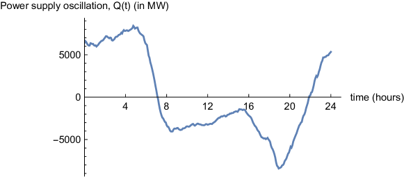
7. Real Data
In this section, we use real data of daily energy consumption in the UK, during a twenty-four hour period. The data is available online at https://www.nationalgrid.com/uk/. In Figure 1, we plot the power supply oscillation (which is simply the negative of the demand) normalized to have mean zero over 24 hours.
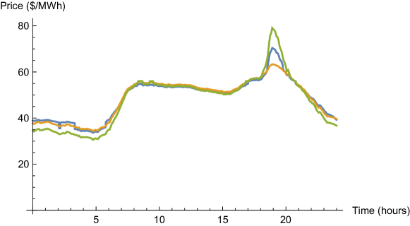
We compare our price-formation model with the MFG model presented in [9]. In that model, the energy price is a function of the aggregate consumption. In that case, the price is not determined by a supply vs demand condition and, thus, there may be an energy imbalance. Here, we consider the state-independent quadratic cost model from Section 6.1. In our model, the price depends only on the constant that accounts for battery’s wear and tear. This constant can be empirically estimated, but, here, we calibrate our model against the model in [9] using a least squares approach. Let be the priced computed in [9]. According to (25), the price given is . Thus, we estimate the value of , by solving the minimization problem
| (36) |
and, using agents, we obtained .
The price given by our model is plotted in Figure 2. We predict smaller peak oscillations and thus, our methods may help stabilize the market.
8. Conclusions and extensions
Here, we described a model for price formation in electricity markets, proved the well-posedness of the problem, and developed methods to compute the solutions. Our model has a minimal number of features and fits well real data. In addition, our model may have stabilizing properties of the price at peak consumption.
Several extensions of our model are of interest. First, we can consider the case where the supply depends on price. Provided the supply increases with the price, which is a natural assumption from the economic point of view, the solvability conditions are similar. In particular, (18) becomes
Thus, we obtain similar bounds for if . Therefore, the existence theory follows a similar argument. Moreover, if , the operator in section (5) is monotone and, therefore, uniqueness of solution holds.
In real applications, may depend on delayed prices. While this does not fit directly into our framework, we can consider a Taylor expansion:
Thus, it is natural to look at the case where depends on the price and its derivatives.
Finally, a natural extension is the case where has random fluctuations. This is particularly relevant if the energy production is subject to unpredictable changes - this is the case of wind energy. For the case where is random, we need to use the master equation as in [25].
References
- [1] M. Bardi and I. Capuzzo-Dolcetta. Optimal control and viscosity solutions of Hamilton-Jacobi-Bellman equations. Birkhäuser Boston Inc., Boston, MA, 1997. With appendices by Maurizio Falcone and Pierpaolo Soravia.
- [2] M. Burger, L. A. Caffarelli, P. A. Markowich, and M.-T. Wolfram. On the asymptotic behavior of a Boltzmann-type price formation model. Commun. Math. Sci., 12(7):1353–1361, 2014.
- [3] M. Burger, L. A. Caffarelli, P. A. Markowich, and Marie-Therese Wolfram. On a Boltzmann-type price formation model. Proc. R. Soc. Lond. Ser. A Math. Phys. Eng. Sci., 469(2157):20130126, 20, 2013.
- [4] L. A. Caffarelli, P. A. Markowich, and J.-F. Pietschmann. On a price formation free boundary model by Lasry and Lions. C. R. Math. Acad. Sci. Paris, 349(11-12):621–624, 2011.
- [5] L. A. Caffarelli, P. A. Markowich, and M.-T. Wolfram. On a price formation free boundary model by Lasry and Lions: the Neumann problem. C. R. Math. Acad. Sci. Paris, 349(15-16):841–844, 2011.
- [6] P. Cardaliaguet. Notes on mean-field games. 2011.
- [7] A. Clemence, B. Tahar Imen, and M. Anis. An Extended Mean Field Game for Storage in Smart Grids. ArXiv e-prints, October 2017.
- [8] R. Couillet, S. Medina Perlaza, H. Tembine, and M. Debbah. Electrical Vehicles in the Smart Grid: A Mean Field Game Analysis. ArXiv e-prints, October 2011.
- [9] A. De Paola, D. Angeli, and G. Strbac. Distributed control of micro-storage devices with mean field games. IEEE Transactions on Smart Grid, 7(2):1119–1127, 2016.
- [10] L. C. Evans. Adjoint and compensated compactness methods for Hamilton-Jacobi PDE. Arch. Ration. Mech. Anal., 197(3):1053–1088, 2010.
- [11] D. Gomes, L. Lafleche, and L. Nurbekyan. A mean-field game economic growth model. Proceedings of the American Control Conference, 2016-July:4693–4698, 2016.
- [12] D. Gomes, L. Nurbekyan, and E. Pimentel. Economic models and mean-field games theory. Publicações Matemáticas do IMPA. [IMPA Mathematical Publications]. Instituto Nacional de Matemática Pura e Aplicada (IMPA), Rio de Janeiro, 2015. 30 Colóquio Brasileiro de Matemática. [30th Brazilian Mathematics Colloquium].
- [13] D. Gomes, E. Pimentel, and V. Voskanyan. Regularity theory for mean-field game systems. SpringerBriefs in Mathematics. Springer, [Cham], 2016.
- [14] D. Gomes and J. Saúde. Mean field games models—a brief survey. Dyn. Games Appl., 4(2):110–154, 2014.
- [15] Olivier Guéant, Jean Michel Lasry, and Pierre Louis Lions. Mean Field Games and Oil Production. 2010.
- [16] M. Huang, P. E. Caines, and R. P. Malhamé. Large-population cost-coupled LQG problems with nonuniform agents: individual-mass behavior and decentralized -Nash equilibria. IEEE Trans. Automat. Control, 52(9):1560–1571, 2007.
- [17] M. Huang, R. P. Malhamé, and P. E. Caines. Large population stochastic dynamic games: closed-loop McKean-Vlasov systems and the Nash certainty equivalence principle. Commun. Inf. Syst., 6(3):221–251, 2006.
- [18] A.C. Kizilkale and R.P. Malhame. A class of collective target tracking problems in energy systems: Cooperative versus non-cooperative mean field control solutions. Proceedings of the IEEE Conference on Decision and Control, 2015-February(February):3493–3498, 2014.
- [19] A.C. Kizilkale and R.P. Malhame. Collective target tracking mean field control for electric space heaters. 2014 22nd Mediterranean Conference on Control and Automation, MED 2014, pages 829–834, 2014.
- [20] A.C. Kizilkale and R.P. Malhame. Collective target tracking mean field control for markovian jump-driven models of electric water heating loads. IFAC Proceedings Volumes (IFAC-PapersOnline), 19:1867–1872, 2014.
- [21] Aimé Lachapelle, Jean-Michel Lasry, Charles-Albert Lehalle, and Pierre-Louis Lions. Efficiency of the price formation process in presence of high frequency participants: a mean field game analysis. Math. Financ. Econ., 10(3):223–262, 2016.
- [22] J.-M. Lasry and P.-L. Lions. Jeux à champ moyen. I. Le cas stationnaire. C. R. Math. Acad. Sci. Paris, 343(9):619–625, 2006.
- [23] J.-M. Lasry and P.-L. Lions. Jeux à champ moyen. II. Horizon fini et contrôle optimal. C. R. Math. Acad. Sci. Paris, 343(10):679–684, 2006.
- [24] J.-M. Lasry and P.-L. Lions. Mean field games. Jpn. J. Math., 2(1):229–260, 2007.
- [25] P. L. Lions. Collège de France course on mean-field games. 2007-2011.
- [26] Roland Malhamé and Chee-Yee Chong. On the statistical properties of a cyclic diffusion process arising in the modeling of thermostat-controlled electric power system loads. SIAM J. Appl. Math., 48(2):465–480, 1988.
- [27] Roland Malhamé, Sofiène Kamoun, and Denis Dochain. On-line identification of electric load models for load management. In Advances in computing and control (Baton Rouge, LA, 1988), volume 130 of Lect. Notes Control Inf. Sci., pages 290–304. Springer, Berlin, 1989.
- [28] P. A. Markowich, N. Matevosyan, J.-F. Pietschmann, and M.-T. Wolfram. On a parabolic free boundary equation modeling price formation. Math. Models Methods Appl. Sci., 19(10):1929–1957, 2009.