Energy-Stable Boundary Conditions Based on a Quadratic Form: Applications to Outflow/Open-Boundary Problems in Incompressible Flows

Abstract

We present a set of new energy-stable open boundary conditions for tackling the backflow instability in simulations of outflow/open boundary problems for incompressible flows. These boundary conditions are developed through two steps: (i) devise a general form of boundary conditions that ensure the energy stability by re-formulating the boundary contribution into a quadratic form in terms of a symmetric matrix and computing an associated eigen problem; and (ii) require that, upon imposing the boundary conditions from the previous step, the scale of boundary dissipation should match a physical scale. These open boundary conditions can be re-cast into the form of a traction-type condition, and therefore they can be implemented numerically using the splitting-type algorithm from a previous work. The current boundary conditions can effectively overcome the backflow instability typically encountered at moderate and high Reynolds numbers. These boundary conditions in general give rise to a non-zero traction on the entire open boundary, unlike previous related methods which only take effect in the backflow regions of the boundary. Extensive numerical experiments in two and three dimensions are presented to test the effectiveness and performance of the presented methods, and simulation results are compared with the available experimental data to demonstrate their accuracy.

Keywords: energy stability; energy stable boundary condition; energy balance; backflow instability; open boundary condition; outflow boundary condition;

1 Introduction

Outflow/open-boundary problems are an important and challenging class of problems for incompressible flow simulations. Several types of flows that are of practical engineering/biological significance and fundamental physical interest belong to this class, such as wakes, jets, shear layers, cardiovascular and respiratory flows. The predominant challenge in the numerical simulations of such problems lies in the treatment of the outflow or open boundary Gresho1991 ; SaniG1994 . If the Reynolds number is low, a number of types of open/outflow boundary conditions (OBC) can work well and lead to reasonable simulation results. But when the Reynolds number increases beyond some moderate value, typically close to $2000$ (which can be as low as several hundred depending on the flow geometry), the so-called backflow instability (see e.g. Dong2015obc ) will become a severe issue, and many open boundary conditions that work well for low Reynolds numbers cease to work. Backflow instability refers to the numerical instability caused by the un-controlled energy influx into the domain through the open/outflow boundary, often associated with strong vortices or backflows on such boundaries. A telltale symptom of this instability is that an otherwise stable computation blows up instantly when a vortex reaches the open/outflow boundary DongK2005 ; DongKER2006 ; VargheseFF2007 ; GhaisasSF2015 . It is observed that usual measures such as increasing the mesh resolution or reducing the time step size do not help with this instability DongKC2014 .

To tackle the backflow instability, the energy influx into the domain through the open boundary, if any, must be controlled in some fashion. Employing a large enough computational domain such that vortices can be sufficiently dissipated before reaching the outflow/open boundary, or artificially increasing the viscosity in a region near/at the outflow boundary (so-called sponge) such that vortices can be smoothed out or sufficiently weakened, are some measures in actual simulations. These measures may not be desirable in terms of e.g. the increased computational cost due to the larger domain or the negative influence on the accuracy due to the artificially modified viscosity in regions of the flow, and additionally they may not always be effective with the increase of Reynolds number.

How to algorithmically control the energy influx through the open boundary by devising effective open boundary conditions seems a more attractive approach. A number of researchers have contributed to this area, and there appears to be a surging interest in recent years. In the early works (see e.g. BruneauF1994 ; BruneauF1996 ) the traction on the open boundary is modified to include a term $\frac{1}{2}(\mathbf{n}\cdot\mathbf{u})^{-}\mathbf{u}$, where $\mathbf{u}$ and $\mathbf{n}$ are respectively the velocity on and the directional unit vector of the boundary, and $(\mathbf{n}\cdot\mathbf{u})^{-}$ is equal to $\mathbf{n}\cdot\mathbf{u}$ if $\mathbf{n}\cdot\mathbf{u}<0$ and zero otherwise. This open boundary condition has also appeared or is studied in some later works; see e.g. LanzendorferS2011 ; FeistauerN2013 ; Fouchet2014 ; BraackM2014 among others. A variant of this form, with a term $(\mathbf{n}\cdot\mathbf{u})^{-}\mathbf{u}$ in the traction (without the $1/2$ factor), has been investigated in a number of works (see e.g. BazilevsGHMZ2009 ; Moghadametal2011 ; PorporaZVP2012 ; GravemeierCYIW2012 ; IsmailGCW2014 ). It is noted that in Moghadametal2011 a form $\beta(\mathbf{n}\cdot\mathbf{u})^{-}\mathbf{u}$, with a constant $0<\beta<1$, has also been considered. In DongKC2014 an open boundary condition with a modified traction term $\left[\frac{1}{2}|\mathbf{u}|^{2}\mathbf{n}\right]\Theta_{0}(\mathbf{n},\mathbf{u})$ is suggested, where $\Theta_{0}(\mathbf{n},\mathbf{u})$ is a smoothed step function essentially taking the unit value if $\mathbf{n}\cdot\mathbf{u}<0$ and vanishing otherwise. So this additional traction term only takes effect in regions of backflow on the open boundary, and has no effect in normal outflow regions or if no backflow is present. Note that this is very different from the total pressure ($p+\frac{1}{2}|\mathbf{u}|^{2}$, where $p$ denotes the normalized static pressure) as discussed in e.g. HeywoodRT1996 , which can lead to a similar term $\frac{1}{2}|\mathbf{u}|^{2}\mathbf{n}$ on the boundary. Unlike that of DongKC2014 , this term in the total pressure precludes the energy from exiting the domain even in normal outflow situations, which results in poor and unphysical simulation results HeywoodRT1996 . In contrast, the boundary condition of DongKC2014 has been shown to ensure the energy stability on the open boundary and that it produces accurate simulation results for outflow problems. In DongS2015 a general form of open boundary conditions that ensure the energy stability on the open boundary for incompressible flows has been proposed. This form contains those of BruneauF1994 ; BazilevsGHMZ2009 ; GravemeierCYIW2012 ; IsmailGCW2014 ; DongKC2014 as particular cases. More importantly, the general form suggests other forms of energy-stable open boundary conditions involving terms such as $\frac{1}{4}\left[|\mathbf{u}|^{2}\mathbf{n}+(\mathbf{n}\cdot\mathbf{u})\mathbf{u}\right]\Theta_{0}(\mathbf{n},\mathbf{u}),$ $\frac{1}{2}\left[|\mathbf{u}|^{2}\mathbf{n}+(\mathbf{n}\cdot\mathbf{u})\mathbf{u}\right]\Theta_{0}(\mathbf{n},\mathbf{u}),$ and $\left[|\mathbf{u}|^{2}\mathbf{n}\right]\Theta_{0}(\mathbf{n},\mathbf{u}).$ Several of these forms have been studied in detail in DongS2015 . It is observed that the term $(\mathbf{n}\cdot\mathbf{u})\mathbf{u}$ (with or without the $1/2$ factor) in the OBC tends to cause the vortices to move laterally as they cross the open boundary, while the term $|\mathbf{u}|^{2}\mathbf{n}$ tends to have the effect of squeezing the vortices along the direction normal to the open boundary. In Dong2015obc a convective-like energy-stable open boundary condition is proposed, which contains an inertia term (velocity time-derivative) and represents a Newton’s second-law type relation on the open boundary. Under certain situations it can be reduced to a form that is reminiscent of the usual convective boundary condition, hence the name “convective-like” condition. This OBC not only ensures the energy stability but also provides a control over the velocity on the outflow/open boundary. It is observed in Dong2015obc that the inertia term in this OBC allows the vortices to discharge from the domain in a more smooth and natural fashion, when compared with the previous energy-stable OBCs without the inertia term (see e.g. those of DongS2015 ). A generalization of this condition to other forms of convective-like energy-stable OBCs has also been provided in Dong2015obc . Besides the above methods, other open boundary conditions that can work with the backflow instability also exist. We refer the reader to e.g. those of BertoglioC2014 ; BertoglioC2016 which are given based on a weak formulation of the Navier-Stokes equations, and also to Bertoglioetal2018 for a recent study of several methods in the context of physiological flows. We also refer to Dong2014obc ; DongW2016 ; YangD2018 for methods dealing with two-phase and multiphase outflows and open boundaries and related issues.

The principle for addressing the backflow instability issue lies in the management and control of the boundary contribution of the open boundary to the energy balance of the system. A key strategy for achieving this is to devise boundary conditions such that the boundary contribution to the energy balance is dissipative (i.e. negative semi-definite) on the open/outflow boundary. This strategy has been employed in the developments of DongKC2014 ; DongS2015 ; Dong2015obc and several other afore-mentioned methods. Recently, a more systematic roadmap to formulating boundary conditions to ensure the definiteness of the boundary contribution (in the context of compressible Navier-Stokes equations) is proposed in Nordstrom2017 . This roadmap involves three main steps: (i) reformulate the boundary contribution into a quadratic form in terms of a symmetric matrix, (ii) rotate the variables to diagonalize the matrix, and (iii) formulate the boundary condition in the form of the eigen-variables corresponding to the negative eigenvalues expressed in terms of the eigen-variables corresponding to the positive eigenvalues. This procedure is very recently applied in NordstromC2018 to the incompressible Navier-Stokes equations in two dimensions to investigate the boundary conditions on solid walls and far fields that can bound the energy of the system.

Inspired by the works of Nordstrom2017 ; NordstromC2018 , we develop in this paper a set of new open/outflow boundary conditions for tackling the backflow instability for incompressible flows in two and three dimensions based on the procedure of Nordstrom2017 . By formulating the boundary integral term in the energy balance equation into a quadratic form involving a symmetric matrix, we have derived a general form of boundary conditions that ensure the energy dissipation on the open boundary. It should be pointed out that, due to differences in the formulation of the quadratic form and the symmetric matrix involved therein, the energy-stable boundary conditions obtained here are different from those of NordstromC2018 , even though the procedure used for deriving the boundary conditions is similar.

We find that the energy-stable boundary conditions as devised above based on the quadratic form can be re-formulated equivalently into a traction-type condition similar to those of DongKC2014 ; DongS2015 , albeit involving a different traction term. More importantly, we observe that the boundary conditions as obtained above in general give rise to poor or even unphysical results in numerical simulations of outflow problems, even though the computations are indeed stable, unless the algorithmic parameters take certain values for the given flow problem under study. We further observe that the values for the algorithmic parameters that can lead to “good” simulation results, unfortunately, are flow-problem dependent.

An investigation of this issue reveals that the resultant dissipation on the open boundary after imposing these boundary conditions is crucial to and strongly influences the accuracy of simulation results. By requiring that the scale of the boundary dissipation on the open boundary should match a reasonable physical scale, we attain a set of open boundary conditions in two and three dimensions that can effectively overcome the backflow instability and also provide accurate simulation results. This set of new open boundary conditions is different from and not equivalent to the family of conditions developed in DongS2015 ; DongKC2014 . For one thing, the new boundary conditions are active (i.e. leading to generally non-zero traction) on the entire open boundary, in both backflow regions and normal outflow regions. In contrast, the previous methods only take effect in the backflow regions of the open boundary, and give rise to a zero traction in normal outflow regions due to the terms like $\Theta_{0}(\mathbf{n},\mathbf{u})$ or $(\mathbf{n}\cdot\mathbf{u})^{-}$.

Therefore, the current energy-stable open boundary conditions with physical accuracy are developed through two steps: (i) devise energy-stable boundary conditions based on a quadratic form in terms of a symmetric matrix, using the procedure of Nordstrom2017 ; (ii) require that the boundary dissipation with these conditions should match a physical scale. The boundary conditions resulting from the first step only can lead to poor or even unphysical simulation results, even though the computations are stable.

The contribution of this paper lies in the set of energy-stable and physically-accurate open boundary conditions developed herein for incompressible flows. These open boundary conditions can be implemented numerically with the commonly-used splitting-type schemes for the incompressible Navier-Stokes equations. This is because the current conditions are formulated in a traction form, similar to those of DongKC2014 ; DongS2015 . This allows us to employ any of the algorithms developed in the previous works (see DongKC2014 ; DongS2015 ; Dong2015obc ) for simulations with the new open boundary conditions. For the numerical experiments reported in the current work, the algorithm from Dong2015obc has been employed.

The current implementation of these open boundary conditions is based on the $C^{0}$-continuous spectral element method SherwinK1995 ; KarniadakisS2005 ; ZhengD2011 , similar to previous works DongKC2014 ; DongS2015 ; Dong2015obc . It should be pointed out that these boundary conditions are given on the continuum level, irrespective of the numerical methods employed for their implementation. They can also be used with other popular techniques such as finite difference, finite element, or finite volume methods.

The rest of this paper is organized as follows. In Section 2 we first derive the general forms of energy-stable boundary conditions, referred to as OBC-A, based on the method of quadratic forms in two and three dimensions. Then we impose the requirement that the scale of boundary dissipation upon imposing these conditions should match a physical scale, and thus acquire another set of open boundary conditions. Two boundary conditions among this set, referred to as OBC-B and OBC-C, are studied in more detail. The numerical implementation of these boundary conditions is also discussed. In Section 3 we present extensive numerical simulations using two canonical flows, the flow past a circular cylinder in two and three dimensions and a jet impinging on a wall in two dimensions, to test the accuracy and performance of the three open boundary conditions OBC-A, OBC-B and OBC-C. Section 4 concludes the presentation with discussions and some closing remarks. In Appendix A we provide a proof of Theorem 2.1 used in Section 2 for the derivation of energy-stable boundary conditions. Appendix B provides a summary of the numerical algorithm from Dong2015obc , and provides some details on the numerical implementation of the open boundary conditions developed in the main text of the paper.

2 Energy-Stable Boundary Conditions for Incompressible Navier-Stokes Equations

2.1 Navier-Stokes Equations and Energy Balance Relation

Consider a flow domain $\Omega$ in two or three dimensions, whose boundary is denoted by $\partial\Omega$, and an incompressible flow on this domain. Let $L$ denote a length scale, $U_{0}$ denote a velocity scale, and $\nu_{f}$ denote the kinematic viscosity of the fluid. The flow is described by the normalized incompressible Navier-Stokes equations,

$$\frac{\partial\mathbf{u}}{\partial t}+\mathbf{u}\cdot\nabla\mathbf{u}+\nabla p-\nu\nabla^{2}\mathbf{u}=\mathbf{f},$$ (1a)

$$\nabla\cdot\mathbf{u}=0,$$ (1b)

where $\mathbf{u}(\mathbf{x},t)$ is the velocity, $p(\mathbf{x},t)$ is the pressure, $\mathbf{f}(\mathbf{x},t)$ is an external body force, and $\mathbf{x}$ and $t$ are the spatial coordinate and time, respectively. $\nu$ is the non-dimensional viscosity, given by

$$\nu=\frac{1}{Re}=\frac{\nu_{f}}{U_{0}L},$$ (2)

where $Re$ is the Reynolds number.

The equations (1a)–(1b) are to be supplemented by appropriate boundary conditions on $\partial\Omega$, which is the focus of this work in subsequent sections, together with the following initial condition for the velocity

$$\mathbf{u}(\mathbf{x},0)=\mathbf{u}_{in}(\mathbf{x}),$$ (3)

where $\mathbf{u}_{in}$ is the initial velocity distribution satisfying equation (1b) and compatible with the boundary condition on $\partial\Omega$.

Taking the $L^{2}$ inner product between (1a) and $\mathbf{u}$ and using the integration by part, the divergence theorem and equation (1b), we arrive at the following energy-balance equation

$$\frac{\partial}{\partial t}\int_{\Omega}\frac{1}{2}|\mathbf{u}|^{2}=\int_{\Omega}\mathbf{f}\cdot\mathbf{u}-\nu\int_{\Omega}\left\|\nabla\mathbf{u}\right\|^{2}+\int_{\partial\Omega}\underbrace{\left[\mathbf{n}\cdot\mathbf{T}\cdot\mathbf{u}-\frac{1}{2}(\mathbf{u}\cdot\mathbf{u})(\mathbf{n}\cdot\mathbf{u})\right]}_{\text{boundary term (BT)}},$$ (4)

where $\mathbf{n}$ is the outward-pointing unit vector normal to $\partial\Omega$, $\mathbf{T}=-p\mathbf{I}+\nu\nabla\mathbf{u}$ and $\mathbf{I}$ is the identity tensor. $\mathbf{T}$ can be roughly considered as the fluid stress tensor. If the external body force is absent ($\mathbf{f}=0$), the volume integral term on the right hand side (RHS) of the above equation is always dissipative and will not cause the system energy to increase over time. The surface integral term, on the other hand, is indefinite. Its contribution to the system energy will depend on the boundary conditions imposed on the domain boundary.

2.2 Energy-Stable Boundary Conditions Based on a Quadratic Form

We are interested in the boundary conditions on $\partial\Omega$ such that the boundary integral term on RHS of the energy balance equation (4) will always be non-positive. As such, the contribution of the surface integral will not cause the system energy to increase over time. Such boundary conditions are referred to as energy-stable boundary conditions.

Inspired by the strategy of Nordstrom2017 to enforce the definiteness of the boundary contribution, we will first reformulate the the boundary integral term in (4) into a quadratic form in terms of a symmetric matrix. Then by looking into the eigenvalues and the associated eigenvectors of this matrix, we formulate the boundary condition in the form of a relation between those eigenvariables corresponding to the eigenvalues of different signs. By imposing a proper condition on the coefficients involved in this relation, the boundary condition can guarantee the negative semi-definiteness of the quadratic form.

The following property about a particular form of symmetric matrices will be extensively used subsequently:

Theorem 2.1.

Let $\mathbf{G}$ denote an $m\times m$ ($m\geqslant 1$) real symmetric matrix, $\mathbf{I}_{m}$ denote the $m\times m$ identity matrix, and $\mathbf{A}=\begin{bmatrix}\mathbf{0}&-\mathbf{I}_{m}\\ -\mathbf{I}_{m}&\mathbf{G}\end{bmatrix}.$ Then

1. The eigenvalues of $\mathbf{A}$ are real and non-zero.

2. $\lambda$ is an eigenvalue of $\mathbf{A}$ if and only if $\left(\lambda-\frac{1}{\lambda}\right)$ is an eigenvalue of $\mathbf{G}$.

3. $\begin{bmatrix}\mathbf{Z}\\ -\lambda\mathbf{Z}\end{bmatrix}$ is an eigenvector of $\mathbf{A}$ corresponding to the eigenvalue $\lambda$ if and only if $\mathbf{Z}$ is an eigenvector of $\mathbf{G}$ corresponding to the eigenvalue $\left(\lambda-\frac{1}{\lambda}\right)$.

A proof of this property is provided in the Appendix A. This theorem suggests that the eigenvalues and the eigenvectors of the $2m\times 2m$ matrix $\mathbf{A}$ can be constructed based on those of the $m\times m$ matrix $\mathbf{G}$. Let $\xi$ denote an eigenvalue (real) of the symmetric matrix $\mathbf{G}$. Then the corresponding eigenvalues of matrix $\mathbf{A}$ are given by $\lambda=\frac{\xi}{2}\pm\sqrt{\left(\frac{\xi}{2}\right)^{2}+1}.$ Therefore, half of the eigenvalues of $\mathbf{A}$ are positive and half are negative.

2.2.1 Two Dimensions (2D)

We first consider two dimensions in space. Let $\mathbf{n}$ and $\bm{\tau}$ denote the unit vectors normal (pointing outward) and tangential to the boundary $\partial\Omega$, respectively, and $\mathbf{n}\times\bm{\tau}=\mathbf{e}_{z}$, where $\mathbf{e}_{z}$ denotes the unit vector along the third (i.e. $z$) direction normal to the two-dimensional plane. Define the normal and tangent components of the fluid stress and the velocity on the boundary by

$$T_{nn}=\mathbf{n}\cdot\mathbf{T}\cdot\mathbf{n},\quad T_{n\tau}=\mathbf{n}\cdot\mathbf{T}\cdot\bm{\tau},\quad u_{n}=\mathbf{n}\cdot\mathbf{u},\quad u_{\tau}=\bm{\tau}\cdot\mathbf{u},\quad\text{on}\ \partial\Omega.$$ (5)

Note that $\mathbf{u}=u_{n}\mathbf{n}+u_{\tau}\bm{\tau}$, and $\mathbf{n}\cdot\mathbf{T}=T_{nn}\mathbf{n}+T_{n\tau}\bm{\tau}$ on $\partial\Omega$. The boundary term in equation (4) can then be written as a quadratic form with a symmetric matrix $\mathbf{A}$ as follows,

$$\text{BT}=-\frac{1}{2}\begin{bmatrix}T_{nn}\\ T_{n\tau}\\ u_{n}\\ u_{\tau}\end{bmatrix}^{T}\underbrace{\begin{bmatrix}0&0&-1&0\\ 0&0&0&-1\\ -1&0&u_{n}&\alpha u_{\tau}\\ 0&-1&\alpha u_{\tau}&\beta u_{n}\end{bmatrix}}_{\text{matrix}\ \mathbf{A}}\underbrace{\begin{bmatrix}T_{nn}\\ T_{n\tau}\\ u_{n}\\ u_{\tau}\end{bmatrix}}_{\mathbf{X}}=-\frac{1}{2}\mathbf{X}^{T}\mathbf{AX},$$ (6)

where the superscript in $(\cdot)^{T}$ denotes transpose, $\alpha$ a chosen constant satisfying $0\leqslant\alpha\leqslant\frac{1}{2}$, and $\beta=1-2\alpha$. This matrix has the form as given by Theorem 2.1 with $m=2$, and in this case

$$\mathbf{G}=\begin{bmatrix}u_{n}&\alpha u_{\tau}\\ \alpha u_{\tau}&\beta u_{n}\end{bmatrix}.$$ (7)

In what follows, we distinguish two cases: (i) $0<\alpha\leqslant\frac{1}{2}$, and (ii) $\alpha=0$, and treat them individually.

Case $0<\alpha\leqslant\frac{1}{2}$.

The matrix $\mathbf{A}$ defined in (6) has four distinct eigenvalues,

$$\left\{\begin{array}[]{ll}\lambda_{1}=\frac{\xi_{1}}{2}-\sqrt{\left(\frac{\xi_{1}}{2}\right)^{2}+1},&\lambda_{2}=\frac{\xi_{2}}{2}-\sqrt{\left(\frac{\xi_{2}}{2}\right)^{2}+1},\\ \lambda_{3}=\frac{\xi_{1}}{2}+\sqrt{\left(\frac{\xi_{1}}{2}\right)^{2}+1},&\lambda_{4}=\frac{\xi_{2}}{2}+\sqrt{\left(\frac{\xi_{2}}{2}\right)^{2}+1},\end{array}\right.$$ (8)

where $\xi_{1}$ and $\xi_{2}$ are the eigenvalues of the matrix $\mathbf{G}$ defined in (7),

$$\left\{\begin{split}&\xi_{1}=(1-\alpha)u_{n}+\alpha\sqrt{u_{n}^{2}+u_{\tau}^{2}}=(1-\alpha)u_{n}+\alpha|\mathbf{u}|\\ &\xi_{2}=(1-\alpha)u_{n}-\alpha\sqrt{u_{n}^{2}+u_{\tau}^{2}}=(1-\alpha)u_{n}-\alpha|\mathbf{u}|,\end{split}\right.$$ (9)

and $|\mathbf{u}|$ denotes the magnitude of the velocity. Note that $\lambda_{1},\lambda_{2}<0$, and $\lambda_{3},\lambda_{4}>0$. The following relations about these eigenvalues will be useful for subsequent discussions,

$$\left\{\begin{split}&1-\lambda_{1}^{2}=-\xi_{1}\lambda_{1},\qquad 1-\lambda_{3}^{2}=-\xi_{1}\lambda_{3};\\ &1-\lambda_{2}^{2}=-\xi_{2}\lambda_{2},\qquad 1-\lambda_{4}^{2}=-\xi_{2}\lambda_{4}.\end{split}\right.$$ (10)

If $|\mathbf{u}|=0$, the contribution of the boundary term in (4) vanishes. So we assume that $|\mathbf{u}|\neq 0$ in the following derivation of the boundary conditions.

The eigenvectors of $\mathbf{G}$ corresponding to the eigenvalues $\xi_{1}$ and $\xi_{2}$ have two representations, given by

$$\left\{\begin{split}&\begin{bmatrix}1\\ \eta\end{bmatrix},\ \ \begin{bmatrix}-\eta\\ 1\end{bmatrix},\ \ \text{if}\ u_{n}\geqslant 0;\\ &\begin{bmatrix}\eta\\ 1\end{bmatrix},\ \ \begin{bmatrix}1\\ -\eta\end{bmatrix},\ \ \text{if}\ u_{n}<0,\end{split}\right.$$ (11)

where

$$\eta=\frac{u_{\tau}}{|\mathbf{u}|+|u_{n}|}.$$ (12)

If $u_{\tau}\neq 0$, both representations of the eigenvectors are equivalent. But when $u_{\tau}=0$ only one of these two representations is suitable, depending on the sign of $u_{n}$ as given above. Based on Theorem 2.1, the four eigenvectors of the matrix $\mathbf{A}$ are given by

$$\begin{bmatrix}1\\ \eta\\ -\lambda_{1}\\ -\eta\lambda_{1}\end{bmatrix},\qquad\begin{bmatrix}-\eta\\ 1\\ \eta\lambda_{2}\\ -\lambda_{2}\end{bmatrix},\qquad\begin{bmatrix}1\\ \eta\\ -\lambda_{3}\\ -\eta\lambda_{3}\end{bmatrix},\qquad\begin{bmatrix}-\eta\\ 1\\ \eta\lambda_{4}\\ -\lambda_{4}\end{bmatrix},\quad\text{if}\ u_{n}\geqslant 0,$$ (13)

and by

$$\begin{bmatrix}\eta\\ 1\\ -\eta\lambda_{1}\\ -\lambda_{1}\end{bmatrix},\qquad\begin{bmatrix}1\\ -\eta\\ -\lambda_{2}\\ \eta\lambda_{2}\end{bmatrix},\qquad\begin{bmatrix}\eta\\ 1\\ -\eta\lambda_{3}\\ -\lambda_{3}\end{bmatrix},\qquad\begin{bmatrix}1\\ -\eta\\ -\lambda_{4}\\ \eta\lambda_{4}\end{bmatrix},\quad\text{if}\ u_{n}>0.$$ (14)

We use the four eigenvectors of $\mathbf{A}$ to form an orthogonal matrix $\hat{\mathbf{P}}$. For $u_{n}\geqslant 0$,

$$\hat{\mathbf{P}}=\underbrace{\begin{bmatrix}1&-\eta&1&-\eta\\ \eta&1&\eta&1\\ -\lambda_{1}&\eta\lambda_{2}&-\lambda_{3}&\eta\lambda_{4}\\ -\eta\lambda_{1}&-\lambda_{2}&-\eta\lambda_{3}&-\lambda_{4}\end{bmatrix}}_{\mathbf{P}}\underbrace{\frac{1}{\sqrt{1+\eta^{2}}}\text{diag}\left(\frac{1}{\sqrt{1+\lambda_{1}^{2}}},\cdots,\frac{1}{\sqrt{1+\lambda_{4}^{2}}}\right)}_{\mathbf{N}}=\mathbf{P}\mathbf{N}$$ (15)

and for $u_{n}<0$,

$$\hat{\mathbf{P}}=\underbrace{\begin{bmatrix}\eta&1&\eta&1\\ 1&-\eta&1&-\eta\\ -\eta\lambda_{1}&-\lambda_{2}&-\eta\lambda_{3}&-\lambda_{4}\\ -\lambda_{1}&\eta\lambda_{2}&-\lambda_{3}&\eta\lambda_{4}\end{bmatrix}}_{\mathbf{P}}\underbrace{\frac{1}{\sqrt{1+\eta^{2}}}\text{diag}\left(\frac{1}{\sqrt{1+\lambda_{1}^{2}}},\cdots,\frac{1}{\sqrt{1+\lambda_{4}^{2}}}\right)}_{\mathbf{N}}=\mathbf{PN}.$$ (16)

Then the matrix $\mathbf{A}$ in (6) can be written as

$$\mathbf{A}=\mathbf{PN}\begin{bmatrix}\lambda_{1}&&&\\ &\lambda_{2}&&\\ &&\lambda_{3}&\\ &&&\lambda_{4}\end{bmatrix}\mathbf{N}^{T}\mathbf{P}^{T}=\mathbf{P}\bm{\Lambda}\mathbf{P}^{T}$$ (17)

where

$$\bm{\Lambda}=\begin{bmatrix}\bm{\Lambda}^{-}&0\\ 0&\bm{\Lambda}^{+}\end{bmatrix},\quad\bm{\Lambda}^{+}=\frac{1}{2(1+\eta^{2})}\text{diag}\left(\frac{1}{\sqrt{(\xi_{1}/2)^{2}+1}},\frac{1}{\sqrt{(\xi_{2}/2)^{2}+1}}\right),\quad\bm{\Lambda}^{-}=-\bm{\Lambda}^{+},$$ (18)

and we have used the relations $\lambda_{1}\lambda_{3}=-1$ and $\lambda_{2}\lambda_{4}=-1$.

The quadratic form in (6) is transformed into

$$\begin{split}BT&=-\frac{1}{2}\mathbf{X}^{T}\mathbf{P}\bm{\Lambda}\mathbf{P}^{T}\mathbf{X}=-\frac{1}{2}\mathbf{W}^{T}\bm{\Lambda}\mathbf{W}=-\frac{1}{2}\begin{bmatrix}(\mathbf{W}^{-})^{T}&(\mathbf{W}^{+})^{T}\end{bmatrix}\begin{bmatrix}\bm{\Lambda}^{-}&0\\ 0&\bm{\Lambda}^{+}\end{bmatrix}\begin{bmatrix}\mathbf{W}^{-}\\ \mathbf{W}^{+}\end{bmatrix}\\ &=-\frac{1}{2}(\mathbf{W}^{-})^{T}\bm{\Lambda}^{-}\mathbf{W}^{-}-\frac{1}{2}(\mathbf{W}^{+})^{T}\bm{\Lambda}^{+}\mathbf{W}^{+}\end{split}$$ (19)

where

$$\mathbf{W}=\mathbf{P}^{T}\mathbf{X}=\begin{bmatrix}\mathbf{W}^{-}\\ \mathbf{W}^{+}\end{bmatrix}.$$ (20)

Define the matrix formed by the eigenvectors of $\mathbf{G}$ as

$$\mathbf{S}=\left\{\begin{split}&\begin{bmatrix}1&-\eta\\ \eta&1\end{bmatrix},&\text{if}\ u_{n}\geqslant 0,\\ &\begin{bmatrix}\eta&1\\ 1&-\eta\end{bmatrix},&\text{if}\ u_{n}<0.\end{split}\right.$$ (21)

Then $\mathbf{W}^{-}$ and $\mathbf{W}^{+}$ are specifically given by

$$\left\{\begin{split}&\mathbf{W}^{-}=\mathbf{S}^{T}\begin{bmatrix}T_{nn}\\ T_{n\tau}\end{bmatrix}-\begin{bmatrix}\lambda_{1}&\\ &\lambda_{2}\end{bmatrix}\mathbf{S}^{T}\begin{bmatrix}u_{n}\\ u_{\tau}\end{bmatrix},\\ &\mathbf{W}^{+}=\mathbf{S}^{T}\begin{bmatrix}T_{nn}\\ T_{n\tau}\end{bmatrix}-\begin{bmatrix}\lambda_{3}&\\ &\lambda_{4}\end{bmatrix}\mathbf{S}^{T}\begin{bmatrix}u_{n}\\ u_{\tau}\end{bmatrix}.\end{split}\right.$$ (22)

$\mathbf{W}^{-}$ and $\mathbf{W}^{+}$ are the eigenvariables corresponding to the negative and the positive eigenvalues of matrix $\mathbf{A}$, respectively.

Following the strategy of Nordstrom2017 , we consider boundary conditions of the form

$$\mathbf{W}^{-}=\mathbf{RW}^{+},\quad\text{with}\ \mathbf{R}=\begin{bmatrix}a_{11}&a_{12}\\ a_{21}&a_{22}\end{bmatrix}$$ (23)

where $\mathbf{R}$ is a chosen constant matrix satisfying the conditions to be specified below. Substitute these boundary conditions into (19), and the quadratic form becomes

$$BT=-\frac{1}{2}(\mathbf{W}^{+})^{T}\underbrace{\left(\mathbf{R}^{T}\bm{\Lambda}^{-}\mathbf{R}+\bm{\Lambda}^{+}\right)}_{\mathbf{Q}}\mathbf{W}^{+}=-\frac{1}{2}(\mathbf{W}^{+})^{T}\mathbf{QW}^{+}$$ (24)

We require that the matrix $\mathbf{R}$ be chosen such that the matrix $\mathbf{Q}$ as defined above is symmetric positive semi-definite (semi-SPD). As such, the surface integral term in (4) will always be non-positive, and the energy stability of the system is guaranteed. Therefore, equation (23) represents a class of energy-stable boundary conditions.

Let us look into the semi-SPD requirement on $\mathbf{Q}$ in more detail. Let

$$z_{1}=\frac{1}{\sqrt{(\xi_{1}/2)^{2}+1}},\quad z_{2}=\frac{1}{\sqrt{(\xi_{2}/2)^{2}+1}},\quad\mathbf{M}=\text{diag}(z_{1},z_{2}).$$ (25)

In light of (18) and (24), we have $\mathbf{Q}=\frac{1}{2(1+\eta^{2})}\left(-\mathbf{R}^{T}\mathbf{MR}+\mathbf{M}\right).$ Therefore we only need to find constant matrix $\mathbf{R}$ such that the matrix $\mathbf{Q}_{1}=\mathbf{M}-\mathbf{R}^{T}\mathbf{MR}$ be symmetric positive semi-definite for all $u_{n}\in(-\infty,\infty)$, $u_{\tau}\in(-\infty,\infty)$, and $|\mathbf{u}|>0$. Requiring that the eigenvalues of $\mathbf{Q}_{1}$ be non-negative is equivalent to the following conditions:

$$z_{1}(a_{11}^{2}+a_{12}^{2}-1)+z_{2}(a_{21}^{2}+a_{22}^{2}-1)\leqslant 0,$$ (26a)

$$-z_{1}^{2}a_{12}^{2}-z_{2}^{2}a_{21}^{2}+z_{1}z_{2}\left[(a_{11}a_{22}-a_{12}a_{21})^{2}+1-(a_{11}^{2}+a_{22}^{2})\right]\geqslant 0,$$ (26b)

for all $u_{n},u_{\tau}\in(-\infty,\infty)$ and $|\mathbf{u}|>0$. Noting that $z_{1}\in(0,1]$, $z_{2}\in(0,1]$, and $\frac{z_{2}}{z_{1}}\in(0,\infty)$, we conclude that

$$a_{12}=0,\quad a_{21}=0,\quad a^{2}_{11}\leqslant 1,\quad a_{22}^{2}\leqslant 1.$$ (27)

This is one set of conditions the matrix $\mathbf{R}$ must satisfy.

Substituting the expressions of (22) into the boundary conditions (23) leads to

$$(\mathbf{I}_{2}-\mathbf{R})\mathbf{S}^{T}\begin{bmatrix}T_{nn}\\ T_{n\tau}\end{bmatrix}=\left(-\mathbf{R}\begin{bmatrix}\lambda_{3}&\\ &\lambda_{4}\end{bmatrix}+\begin{bmatrix}\lambda_{1}&\\ &\lambda_{2}\end{bmatrix}\right)\mathbf{S}^{T}\begin{bmatrix}u_{n}\\ u_{\tau}\end{bmatrix},$$ (28)

where $\mathbf{I}_{2}$ is the identity matrix of dimension two. We impose the requirement that $(\mathbf{I}_{2}-\mathbf{R})$ be non-singular, i.e.

$$a_{11}\neq 1,\quad a_{22}\neq 1.$$ (29)

This is another set of conditions for $\mathbf{R}$. Equation (28) is then transformed into

$$\begin{split}\begin{bmatrix}T_{nn}\\ T_{n\tau}\end{bmatrix}&=\mathbf{S}^{-T}(\mathbf{I}_{2}-\mathbf{R})^{-1}\left(-\mathbf{R}\begin{bmatrix}\lambda_{3}&\\ &\lambda_{4}\end{bmatrix}+\begin{bmatrix}\lambda_{1}&\\ &\lambda_{2}\end{bmatrix}\right)\mathbf{S}^{T}\begin{bmatrix}u_{n}\\ u_{\tau}\end{bmatrix}=\mathbf{S}^{-T}\begin{bmatrix}K_{1}&\\ &K_{2}\end{bmatrix}\mathbf{S}^{T}\begin{bmatrix}u_{n}\\ u_{\tau}\end{bmatrix}.\end{split}$$ (30)

where

$$K_{1}=\frac{\lambda_{1}-a_{11}\lambda_{3}}{1-a_{11}},\quad K_{2}=\frac{\lambda_{2}-a_{22}\lambda_{4}}{1-a_{22}}.$$ (31)

Substituting the expressions (21) for $\mathbf{S}$ into (30), we have the boundary conditions in the following form. For $u_{n}\geqslant 0$,

$$T_{nn}=\frac{K_{1}+K_{2}\eta^{2}}{1+\eta^{2}}u_{n}+\frac{\eta(K_{1}-K_{2})}{1+\eta^{2}}u_{\tau}=f_{1}(u_{n},u_{\tau}),$$ (32a)

$$T_{n\tau}=\frac{\eta(K_{1}-K_{2})}{1+\eta^{2}}u_{n}+\frac{K_{1}\eta^{2}+K_{2}}{1+\eta^{2}}u_{\tau}=f_{2}(u_{n},u_{\tau}).$$ (32b)

For $u_{n}<0$,

$$T_{nn}=\frac{K_{1}\eta^{2}+K_{2}}{1+\eta^{2}}u_{n}+\frac{\eta(K_{1}-K_{2})}{1+\eta^{2}}u_{\tau}=f_{1}(u_{n},u_{\tau}),$$ (33a)

$$T_{n\tau}=\frac{\eta(K_{1}-K_{2})}{1+\eta^{2}}u_{n}+\frac{K_{1}+K_{2}\eta^{2}}{1+\eta^{2}}u_{\tau}=f_{2}(u_{n},u_{\tau}).$$ (33b)

In the above equations $K_{1}$ and $K_{2}$ are given by (31) and $\eta$ is given by (12). The eigenvalues $\lambda_{i}$ ($1\leqslant i\leqslant 4$) are given by (8). The parameters $a_{11}$ and $a_{22}$ are chosen constants satisfying the following conditions, in light of equations (27) and (29),

$$-1\leqslant a_{11}<1,\quad-1\leqslant a_{22}<1.$$ (34)

These boundary conditions ensure the energy stability of the system.

Let us next look into the boundary term (24) associated with these boundary conditions. The matrix $\mathbf{Q}$ is reduced to $\mathbf{Q}=\frac{1}{2(1+\eta^{2})}\text{diag}\left(z_{1}(1-a_{11}^{2}),z_{2}(1-a_{22}^{2})\right)$ in light of equations (27) and (29). Let $\mathbf{W}^{+}=\begin{bmatrix}W_{1}\\ W_{2}\end{bmatrix}.$ Then we have, in light of equations (22) and (30),

$$\begin{bmatrix}W_{1}\\ W_{2}\end{bmatrix}=\mathbf{W}^{+}=\begin{bmatrix}-\frac{2}{z_{1}(1-a_{11})}&\\ &-\frac{2}{z_{2}(1-a_{22})}\end{bmatrix}\mathbf{S}^{T}\begin{bmatrix}u_{n}\\ u_{\tau}\end{bmatrix}.$$ (35)

Substituting the above expression and the expression (21) into (24), we have

$$BT=\left\{\begin{split}&-\frac{1}{2}\left[\frac{1+a_{11}}{1-a_{11}}\frac{2}{z_{1}(1+\eta^{2})}(u_{n}+\eta u_{\tau})^{2}+\frac{1+a_{22}}{1-a_{22}}\frac{2}{z_{2}(1+\eta^{2})}(-\eta u_{n}+u_{\tau})^{2}\right],\quad\text{if}\ u_{n}\geqslant 0,\\ &-\frac{1}{2}\left[\frac{1+a_{11}}{1-a_{11}}\frac{2}{z_{1}(1+\eta^{2})}(\eta u_{n}+u_{\tau})^{2}+\frac{1+a_{22}}{1-a_{22}}\frac{2}{z_{2}(1+\eta^{2})}(u_{n}-\eta u_{\tau})^{2}\right],\quad\text{if}\ u_{n}<0.\end{split}\right.$$ (36)

According to the above expression, for the boundary conditions given by (32a)–(33b), the amount of dissipation on the boundary is controlled by the parameters $a_{11}$ and $a_{22}$. The larger $a_{11}$ and $a_{22}$ are, the more dissipative these boundary conditions are. When $a_{11}=a_{22}=-1$, the boundary dissipation vanishes completely. In other words, no energy can be convected through the boundary (into or out of the domain) where these boundary conditions are imposed. When $a_{11}\rightarrow 1$ or $a_{22}\rightarrow 1$, the dissipation on the boundary will become infinitely large.

Remark 1.

When deriving the boundary conditions (32a)–(33b), we have assumed that locally $|\mathbf{u}|\neq 0$ on the boundary. The boundary conditions (32a)–(33b), however, can also accommodate the case when $|\mathbf{u}|=0$ locally on the boundary, if we modify the definition of $\eta$ in (12) as follows to make it well defined for $|\mathbf{u}|=0$,

$$\eta=\frac{u_{\tau}}{|\mathbf{u}|+|u_{n}|+\epsilon},$$ (37)

where $\epsilon$ is a small positive number on the order of magnitude of the machine zero or smaller (e.g. $\epsilon=10^{-18}$). With this modified definition for $\eta$, when $\mathbf{u}=0$ locally at any point on the boundary, the boundary conditions are reduced to $T_{nn}=T_{n\tau}=0$.

The boundary conditions (32a)–(33b) can be written into a vector form,

$$\left\{\begin{split}&\mathbf{n}\cdot\mathbf{T}=\mathbf{E}(\mathbf{u},\partial\Omega),\ \text{or}\\ &-p\mathbf{n}+\nu\mathbf{n}\cdot\nabla\mathbf{u}-\mathbf{E}(\mathbf{u},\partial\Omega)=0,\end{split}\right.$$ (38)

where in two dimensions

$$\mathbf{E}(\mathbf{u},\partial\Omega)=f_{1}(u_{n},u_{\tau})\mathbf{n}+f_{2}(u_{n},u_{\tau})\bm{\tau},$$ (39)

and $f_{1}$, $f_{2}$ are given in (32a)–(33b).

Case $\alpha=0$.

The matrix $\mathbf{A}$ has two double eigenvalues,

$$\left\{\begin{split}&\lambda_{1}=\lambda_{2}=\frac{u_{n}}{2}-\sqrt{\left(\frac{u_{n}}{2}\right)^{2}+1},\\ &\lambda_{3}=\lambda_{4}=\frac{u_{n}}{2}+\sqrt{\left(\frac{u_{n}}{2}\right)^{2}+1}.\end{split}\right.$$ (40)

Note that these eigenvalues satisfy the relation $u_{n}-\lambda_{i}=-\frac{1}{\lambda_{i}}\ (1\leqslant i\leqslant 4).$ The corresponding eigenvectors are

$$\begin{bmatrix}1\\ 0\\ -\lambda_{1}\\ 0\end{bmatrix},\quad\begin{bmatrix}0\\ 1\\ 0\\ -\lambda_{1}\end{bmatrix},\quad\begin{bmatrix}1\\ 0\\ -\lambda_{3}\\ 0\end{bmatrix},\quad\begin{bmatrix}0\\ 1\\ 0\\ -\lambda_{3}\end{bmatrix}.$$ (41)

Matrix $\mathbf{A}$ can then be expressed as

$$\mathbf{A}=\mathbf{P}\bm{\Lambda}\mathbf{P}^{T}=\mathbf{P}\begin{bmatrix}\bm{\Lambda}^{-}&\\ &\bm{\Lambda}^{+}\end{bmatrix}\mathbf{P}^{T},$$ (42)

where

$$\mathbf{P}=\begin{bmatrix}1&0&1&0\\ 0&1&0&1\\ -\lambda_{1}&0&-\lambda_{3}&0\\ 0&-\lambda_{1}&0&-\lambda_{3}\end{bmatrix}=\begin{bmatrix}\mathbf{I}_{2}&\mathbf{I}_{2}\\ -\lambda_{1}\mathbf{I}_{2}&-\lambda_{3}\mathbf{I}_{2}\end{bmatrix},\quad\bm{\Lambda}^{-}=-\bm{\Lambda}^{+}=-\frac{1}{2\sqrt{(u_{n}/2)^{2}+1}}\mathbf{I}_{2}.$$ (43)

Accordingly, the boundary term in (6) is transformed into

$$\begin{split}BT&=-\frac{1}{2}\mathbf{X}^{T}\mathbf{P}\bm{\Lambda}\mathbf{P}^{T}\mathbf{X}=-\frac{1}{2}\mathbf{W}^{T}\bm{\Lambda}\mathbf{W}=-\frac{1}{2}\begin{bmatrix}\mathbf{W}^{-}\\ \mathbf{W}^{+}\end{bmatrix}^{T}\begin{bmatrix}\bm{\Lambda}^{-}&0\\ &\bm{\Lambda}^{+}\end{bmatrix}\begin{bmatrix}\mathbf{W}^{-}\\ \mathbf{W}^{+}\end{bmatrix}\\ &=-\frac{1}{2}\left[(\mathbf{W}^{-})^{T}\bm{\Lambda}^{-}\mathbf{W}^{-}+(\mathbf{W}^{+})^{T}\bm{\Lambda}^{+}\mathbf{W}^{+}\right],\end{split}$$ (44)

where $\mathbf{W}=\mathbf{P}^{T}\mathbf{X}=\begin{bmatrix}\mathbf{W}^{-}\\ \mathbf{W}^{+}\end{bmatrix}.$ $\mathbf{W}^{-}$ and $\mathbf{W}^{+}$ are vectors of dimension two and are given specifically by

$$\left\{\begin{split}&\mathbf{W}^{-}=\begin{bmatrix}T_{nn}\\ T_{n\tau}\end{bmatrix}-\lambda_{1}\begin{bmatrix}u_{n}\\ u_{\tau}\end{bmatrix},\\ &\mathbf{W}^{+}=\begin{bmatrix}T_{nn}\\ T_{n\tau}\end{bmatrix}-\lambda_{3}\begin{bmatrix}u_{n}\\ u_{\tau}\end{bmatrix}.\end{split}\right.$$ (45)

We again introduce boundary conditions in the form of equation (23), where the $2\times 2$ constant matrix $\mathbf{R}=\begin{bmatrix}a_{11}&a_{12}\\ a_{21}&a_{22}\end{bmatrix}$ is to be determined. Therefore, the boundary term in (44) can be transformed into the same form as equation (24), in which the matrix

$$\mathbf{Q}=\mathbf{R}^{T}\bm{\Lambda}^{-}\mathbf{R}+\bm{\Lambda}^{+}=\frac{1}{2\sqrt{(u_{n}/2)^{2}+1}}(\mathbf{I}_{2}-\mathbf{R}^{T}\mathbf{R})$$ (46)

is required to be symmetric positive semi-definite. Requiring that the eigenvalues of $\mathbf{Q}$ be non-negative leads to the following conditions:

$$a_{11}^{2}+a_{12}^{2}+a_{21}^{2}+a_{22}^{2}\leqslant 2,\ \text{and}$$ (47a)

$$a_{11}^{2}+a_{12}^{2}+a_{21}^{2}+a_{22}^{2}\leqslant 1+(a_{11}a_{22}-a_{12}a_{21})^{2}.$$ (47b)

A sufficient condition to guarantee both (47a) and (47b) is

$$a_{11}^{2}+a_{12}^{2}+a_{21}^{2}+a_{22}^{2}\leqslant 1.$$ (48)

This indicates that when $a_{ij}$ ($i,j=1,2$) are chosen to be sufficiently small the matrix $\mathbf{R}$ will guarantee the positive semi-definiteness of the matrix $\mathbf{Q}$ and the non-positivity of the surface integral term in (4).

In light of equation (45), the boundary condition in the form of equation (23) is transformed into

$$(\mathbf{I}-\mathbf{R})\begin{bmatrix}T_{nn}\\ T_{n\tau}\end{bmatrix}=(\lambda_{1}\mathbf{I}-\lambda_{3}\mathbf{R})\begin{bmatrix}u_{n}\\ u_{\tau}\end{bmatrix}.$$ (49)

We impose the requirement that $(\mathbf{I}-\mathbf{R})$ be non-singular, i.e.

$$\mathscr{K}=\text{det}(\mathbf{I}-\mathbf{R})=(1-a_{11})(1-a_{22})-a_{12}a_{21}\neq 0.$$ (50)

This is another condition the matrix $\mathbf{R}$ must satisfy. Consequently, the boundary condition (49) becomes

$$\begin{bmatrix}T_{nn}\\ T_{n\tau}\end{bmatrix}=(\mathbf{I}-\mathbf{R})^{-1}(\lambda_{1}\mathbf{I}-\lambda_{3}\mathbf{R})\begin{bmatrix}u_{n}\\ u_{\tau}\end{bmatrix}.$$ (51)

In component forms they are

$$T_{nn}=\frac{1}{\mathscr{K}}\left[(1-a_{22})(\lambda_{1}-\lambda_{3}a_{11})-\lambda_{3}a_{12}a_{21}\right]u_{n}+\frac{1}{\mathscr{K}}(\lambda_{1}-\lambda_{3})a_{12}u_{\tau}=f_{1}(u_{n},u_{\tau}),$$ (52a)

$$T_{n\tau}=\frac{1}{\mathscr{K}}(\lambda_{1}-\lambda_{3})a_{21}u_{n}+\frac{1}{\mathscr{K}}\left[(1-a_{11})(\lambda_{1}-\lambda_{3}a_{22})-\lambda_{3}a_{12}a_{21}\right]u_{\tau}=f_{2}(u_{n},u_{\tau}),$$ (52b)

where $\mathscr{K}$ is given by (50), $\lambda_{1}$ and $\lambda_{3}$ are given by (40), and the chosen constants $a_{ij}$ ($i,j=1,2$) satisfy the conditions (47a), (47b) and (50). These are the energy-stable boundary conditions for the case $\alpha=0$.

Let us now consider a simplified case: $\mathbf{R}$ is assumed to be a diagonal matrix. The conditions (47a), (47b) and (50) are then reduced to

$$a_{12}=a_{21}=0,\quad-1\leqslant a_{11}<1,\quad-1\leqslant a_{22}<1.$$ (53)

These are the same as those conditions for $\mathbf{R}$ in the case $0<\alpha\leqslant\frac{1}{2}$; see equation (34). The boundary conditions (52a)–(52b) are reduced to

$$\left\{\begin{split}&T_{nn}=\frac{\lambda_{1}-\lambda_{3}a_{11}}{1-a_{11}}u_{n},\\ &T_{n\tau}=\frac{\lambda_{1}-\lambda_{3}a_{22}}{1-a_{22}}u_{\tau}.\end{split}\right.$$ (54)

With the above condition, the boundary term becomes

$$BT=-\frac{1}{2}\sqrt{u_{n}^{2}+4}\left(\frac{1+a_{11}}{1-a_{11}}u_{n}^{2}+\frac{1+a_{22}}{1-a_{22}}u_{\tau}^{2}\right).$$ (55)

For this simplified case, the amount of boundary dissipation is controlled by the constants $a_{11}$ and $a_{22}$. It is more dissipative with increasing $a_{11}$ and $a_{22}$.

The boundary conditions (52a)–(52b) can be cast into the same vectorial form as given by (38), in which $\mathbf{E}(\mathbf{u},\partial\Omega)$ is given by

$$\mathbf{E}(\mathbf{u},\partial\Omega)=f_{1}(u_{n},u_{\tau})\mathbf{n}+f_{2}(u_{n},u_{\tau})\bm{\tau},$$ (56)

where $f_{1}(u_{n},u_{\tau})$ and $f_{2}(u_{n},u_{\tau})$ are defined by (52a) and (52b).

2.2.2 Three Dimensions (3D)

We next consider three dimensions in space. Let $\mathbf{n}$ denote the outward-pointing unit vector normal to the boundary $\partial\Omega$, and $\bm{\tau}$ and $\mathbf{s}$ denote the unit vectors along the two independent directions tangent to $\partial\Omega$, such that $(\mathbf{n},\bm{\tau},\mathbf{s})$ are mutually orthogonal and form a right-handed system. Define the three components along the $(\mathbf{n},\bm{\tau},\mathbf{s})$ directions for the stress vector $\mathbf{n}\cdot\mathbf{T}$ and the velocity $\mathbf{u}$,

$$T_{nn}=\mathbf{n}\cdot\mathbf{T}\cdot\mathbf{n},\quad T_{n\tau}=\mathbf{n}\cdot\mathbf{T}\cdot\bm{\tau},\quad T_{ns}=\mathbf{n}\cdot\mathbf{T}\cdot\mathbf{s},\quad u_{n}=\mathbf{n}\cdot\mathbf{u},\quad u_{\tau}=\bm{\tau}\cdot\mathbf{u},\quad u_{s}=\mathbf{s}\cdot\mathbf{u}.$$ (57)

In three dimensions the boundary term in the energy balance equation can be written as

$$\text{BT}=-\frac{1}{2}\begin{bmatrix}T_{nn}\\ T_{n\tau}\\ T_{ns}\\ u_{n}\\ u_{\tau}\\ u_{s}\end{bmatrix}^{T}\underbrace{\begin{bmatrix}0&0&0&-1&0&0\\ 0&0&0&0&-1&0\\ 0&0&0&0&0&-1\\ -1&0&0&u_{n}&\alpha_{1}u_{\tau}&\alpha_{2}u_{s}\\ 0&-1&0&\alpha_{1}u_{\tau}&\beta_{1}u_{n}&0\\ 0&0&-1&\alpha_{2}u_{s}&0&\beta_{2}u_{n}\end{bmatrix}}_{\text{matrix}\ \mathbf{A}}\underbrace{\begin{bmatrix}T_{nn}\\ T_{n\tau}\\ T_{ns}\\ u_{n}\\ u_{\tau}\\ u_{s}\end{bmatrix}}_{\mathbf{X}}=-\frac{1}{2}\mathbf{X}^{T}\mathbf{AX},$$ (58)

where $\alpha_{1}$ and $\alpha_{2}$ are chosen constants satisfying $0\leqslant\alpha_{1}\leqslant\frac{1}{2}$ and $0\leqslant\alpha_{2}\leqslant\frac{1}{2}$, and $\beta_{1}=1-2\alpha_{1}$ and $\beta_{2}=1-2\alpha_{2}$. The matrix $\mathbf{A}$ has the form as discussed in Theorem 2.1, and in this case $\mathbf{G}=\begin{bmatrix}u_{n}&\alpha_{1}u_{\tau}&\alpha_{2}u_{s}\\ \alpha_{1}u_{\tau}&\beta_{1}u_{n}&0\\ \alpha_{2}u_{s}&0&\beta_{2}u_{n}\end{bmatrix}.$

Let $\xi_{1}$, $\xi_{2}$ and $\xi_{3}$ denote the three (real) eigenvalues of $\mathbf{G}$, and $\mathbf{Z}_{1}$, $\mathbf{Z}_{2}$ and $\mathbf{Z}_{3}$ denote the corresponding orthonormal eigenvectors, and $\mathbf{S}=\begin{bmatrix}\mathbf{Z}_{1}\ \mathbf{Z}_{2}\ \mathbf{Z}_{3}\end{bmatrix}$ denote the orthogonal matrix formed by these eigenvectors. According to Theorem 2.1, the eigenvalues of $\mathbf{A}$ are

$$\left\{\begin{array}[]{lll}\lambda_{1}=\frac{\xi_{1}}{2}-\sqrt{\left(\frac{\xi_{1}}{2}\right)^{2}+1},&\lambda_{2}=\frac{\xi_{2}}{2}-\sqrt{\left(\frac{\xi_{2}}{2}\right)^{2}+1},&\lambda_{3}=\frac{\xi_{3}}{2}-\sqrt{\left(\frac{\xi_{3}}{2}\right)^{2}+1},\\ \lambda_{4}=\frac{\xi_{1}}{2}+\sqrt{\left(\frac{\xi_{1}}{2}\right)^{2}+1},&\lambda_{5}=\frac{\xi_{2}}{2}+\sqrt{\left(\frac{\xi_{2}}{2}\right)^{2}+1},&\lambda_{6}=\frac{\xi_{3}}{2}+\sqrt{\left(\frac{\xi_{3}}{2}\right)^{2}+1}.\end{array}\right.$$ (59)

The corresponding eigenvectors are given by

$$\begin{bmatrix}\mathbf{Z}_{1}\\ -\lambda_{1}\mathbf{Z}_{1}\end{bmatrix},\quad\begin{bmatrix}\mathbf{Z}_{2}\\ -\lambda_{2}\mathbf{Z}_{2}\end{bmatrix},\quad\begin{bmatrix}\mathbf{Z}_{3}\\ -\lambda_{3}\mathbf{Z}_{3}\end{bmatrix},\quad\begin{bmatrix}\mathbf{Z}_{1}\\ -\lambda_{4}\mathbf{Z}_{1}\end{bmatrix},\quad\begin{bmatrix}\mathbf{Z}_{2}\\ -\lambda_{5}\mathbf{Z}_{2}\end{bmatrix},\quad\begin{bmatrix}\mathbf{Z}_{3}\\ -\lambda_{6}\mathbf{Z}_{3}\end{bmatrix}.$$ (60)

Let $\mathbf{C}_{1}=\text{diag}(\lambda_{1},\lambda_{2},\lambda_{3})$, $\mathbf{C}_{2}=\text{diag}(\lambda_{4},\lambda_{5},\lambda_{6})$, and $\mathbf{P}=\begin{bmatrix}\mathbf{S}&\mathbf{S}\\ -\mathbf{SC}_{1}&-\mathbf{SC}_{2}\end{bmatrix}.$ Then matrix $\mathbf{A}$ can be represented as

$$\mathbf{A}=\mathbf{P}\begin{bmatrix}\frac{\lambda_{1}}{1+\lambda_{1}^{2}}&&\\ &\ddots&\\ &&\frac{\lambda_{6}}{1+\lambda_{6}^{2}}\end{bmatrix}\mathbf{P}^{T}=\mathbf{P}\bm{\Lambda}\mathbf{P}^{T}=\mathbf{P}\begin{bmatrix}\bm{\Lambda}^{-}&\mathbf{0}\\ \mathbf{0}&\bm{\Lambda}^{+}\end{bmatrix}\mathbf{P}^{T},$$ (61)

where $\bm{\Lambda}^{-}=-\bm{\Lambda}^{+}=-\text{diag}\left(\frac{1}{2\sqrt{(\xi_{1}/2)^{2}+1}},\frac{1}{2\sqrt{(\xi_{2}/2)^{2}+1}},\frac{1}{2\sqrt{(\xi_{3}/2)^{2}+1}}\right).$

Let

$$\begin{bmatrix}\mathbf{W}^{-}\\ \mathbf{W}^{+}\end{bmatrix}=\mathbf{W}=\mathbf{P}^{T}\mathbf{X}=\begin{bmatrix}\mathbf{S}^{T}&-\mathbf{C}_{1}\mathbf{S}^{T}\\ \mathbf{S}^{T}&-\mathbf{C}_{2}\mathbf{S}^{T}\end{bmatrix}\begin{bmatrix}\mathbf{T}_{n}\\ \mathbf{U}\end{bmatrix}=\begin{bmatrix}\mathbf{S}^{T}\mathbf{T}_{n}-\mathbf{C}_{1}\mathbf{S}^{T}\mathbf{U}\\ \mathbf{S}^{T}\mathbf{T}_{n}-\mathbf{C}_{2}\mathbf{S}^{T}\mathbf{U}\end{bmatrix},$$ (62)

where $\mathbf{T}_{n}=\begin{bmatrix}T_{nn}\\ T_{n\tau}\\ T_{ns}\end{bmatrix}$ and $\mathbf{U}=\begin{bmatrix}u_{n}\\ u_{\tau}\\ u_{s}\end{bmatrix}.$ Analogous to the two-dimensional case, we consider boundary conditions of the form $\mathbf{W}^{-}=\mathbf{R}\mathbf{W}^{+},$ where $\mathbf{R}$ is a chosen $3\times 3$ constant matrix. The boundary term (58) is then transformed into

$$\begin{split}BT&=-\frac{1}{2}\left[(\mathbf{W}^{-})^{T}\bm{\Lambda}^{-}\mathbf{W}^{-}+(\mathbf{W}^{+})^{T}\bm{\Lambda}^{+}\mathbf{W}^{+}\right]=-\frac{1}{2}(\mathbf{W}^{+})^{T}\underbrace{\left[\mathbf{R}^{T}\bm{\Lambda}^{-}\mathbf{R}+\bm{\Lambda}^{+}\right]}_{\mathbf{Q}}\mathbf{W}^{+}\\ &=-\frac{1}{2}(\mathbf{W}^{+})^{T}\mathbf{Q}\mathbf{W}^{+}.\end{split}$$ (63)

We then require that $\mathbf{R}$ be chosen such that the symmetric matrix $\mathbf{Q}=\mathbf{R}^{T}\bm{\Lambda}^{-}\mathbf{R}+\bm{\Lambda}^{+}$ is positive semi-definite to ensure the non-positivity of the boundary term.

Since the closed form for $\xi_{i}$ ($i=1,2,3$) is unknown, it is difficult to determine the general form for the matrix $\mathbf{R}$ that ensures the positive semi-definiteness of $\mathbf{Q}$. In the current work we consider only the following special case for three dimensions: We assume that $\mathbf{R}$ is a diagonal matrix, i.e. $\mathbf{R}=\text{diag}(a_{11},a_{22},a_{33})$. With this assumption, the requirement that $\mathbf{Q}$ be symmetric positive semi-definite leads to the conditions

$$a_{11}^{2}\leqslant 1,\quad a_{22}^{2}\leqslant 1,\quad a_{33}^{2}\leqslant 1.$$ (64)

Substitution of the expressions for $\mathbf{W}^{-}$ and $\mathbf{W}^{+}$ in (62) into the boundary condition leads to

$$(\mathbf{I}_{3}-\mathbf{R})\mathbf{S}^{T}\mathbf{T}_{n}=(\mathbf{C}_{1}-\mathbf{R}\mathbf{C}_{2})\mathbf{S}^{T}\mathbf{U}.$$ (65)

We further require that $(\mathbf{I}_{3}-\mathbf{R})$ be non-singular. With this and the condition (64), we arrive at the matrix $\mathbf{R}$ for this special case,

$$\mathbf{R}=\text{diag}(a_{11},a_{22},a_{33}),\ \text{where}\ -1\leqslant a_{11},a_{22},a_{33}<1.$$ (66)

With this $\mathbf{R}$ matrix the boundary condition (65) becomes

$$\begin{split}\mathbf{T}_{n}=\mathbf{S}(\mathbf{I}_{3}-\mathbf{R})^{-1}(\mathbf{C}_{1}-\mathbf{RC}_{2})\mathbf{S}^{T}\mathbf{U}=\mathbf{S}\begin{bmatrix}\frac{\lambda_{1}-\lambda_{4}a_{11}}{1-a_{11}}&&\\ &\frac{\lambda_{2}-\lambda_{5}a_{22}}{1-a_{22}}&\\ &&\frac{\lambda_{3}-\lambda_{6}a_{33}}{1-a_{33}}\end{bmatrix}\mathbf{S}^{T}\mathbf{U}.\end{split}$$ (67)

Equivalently, it can be written as

$$\begin{bmatrix}T_{nn}\\ T_{n\tau}\\ T_{ns}\end{bmatrix}=\mathbf{L}\begin{bmatrix}u_{n}\\ u_{\tau}\\ u_{s}\end{bmatrix}=\begin{bmatrix}L_{11}u_{n}+L_{12}u_{\tau}+L_{13}u_{s}\\ L_{21}u_{n}+L_{22}u_{\tau}+L_{23}u_{s}\\ L_{31}u_{n}+L_{32}u_{\tau}+L_{33}u_{s}\end{bmatrix}=\begin{bmatrix}g_{1}(u_{n},u_{\tau},u_{s})\\ g_{2}(u_{n},u_{\tau},u_{s})\\ g_{3}(u_{n},u_{\tau},u_{s})\end{bmatrix}$$ (68)

where

$$\begin{bmatrix}L_{11}&L_{22}&L_{33}\\ L_{21}&L_{22}&L_{23}\\ L_{31}&L_{32}&L_{33}\end{bmatrix}=\mathbf{L}=\mathbf{S}\begin{bmatrix}\frac{\lambda_{1}-\lambda_{4}a_{11}}{1-a_{11}}&&\\ &\frac{\lambda_{2}-\lambda_{5}a_{22}}{1-a_{22}}&\\ &&\frac{\lambda_{3}-\lambda_{6}a_{33}}{1-a_{33}}\end{bmatrix}\mathbf{S}^{T}.$$ (69)

In vector form, this boundary condition has the same form as given by (38), but here in three dimensions $\mathbf{E}(\mathbf{u},\partial\Omega)$ is given by

$$\mathbf{E}(\mathbf{u},\partial\Omega)=g_{1}(u_{n},u_{\tau},u_{s})\mathbf{n}+g_{2}(u_{n},u_{\tau},u_{s})\bm{\tau}+g_{3}(u_{n},u_{\tau},u_{s})\mathbf{s},$$ (70)

where $g_{1}$, $g_{2}$ and $g_{3}$ are defined by (68). The boundary term (63) is accordingly transformed into

$$BT=-\frac{1}{2}(\mathbf{S}^{T}\mathbf{U})^{T}\begin{bmatrix}\frac{2(1+a_{11})\sqrt{\left(\xi_{1}/2\right)^{2}+1}}{1-a_{11}}&&\\ &\frac{2(1+a_{22})\sqrt{\left(\xi_{2}/2\right)^{2}+1}}{1-a_{22}}&\\ &&\frac{2(1+a_{33})\sqrt{\left(\xi_{3}/2\right)^{2}+1}}{1-a_{33}}\end{bmatrix}(\mathbf{S}^{T}\mathbf{U}).$$ (71)

This expression indicates that the dissipativeness of the boundary condition (68) is controlled by the coefficients $a_{ii}$ ($i=1,2,3$). The larger the values for $a_{ii}$, the more dissipative the boundary condition is. When $a_{11}=a_{22}=a_{33}=-1$, the boundary dissipation vanishes. When $a_{ii}\rightarrow 1$ ($i=1,2,3$), the boundary dissipation approaches infinity.

In summary, the procedure for computing $\mathbf{E}(\mathbf{u},\partial\Omega)$ in the 3D boundary condition is as follows. Given domain boundary $\partial\Omega$ (with normal and tangent vectors $\mathbf{n}$, $\bm{\tau}$, $\mathbf{s}$), the velocity $\mathbf{u}$ on $\partial\Omega$, the chosen constants $a_{ii}$ ($i=1,2,3$), $\alpha_{1}$ and $\alpha_{2}$, we take the following steps:

• Compute $u_{n}$, $u_{\tau}$, $u_{s}$ based on equation (57);

• Form matrix $\mathbf{G}$. Compute the eigenvalues $\xi_{i}$ ($i=1,2,3$) and the eigenvectors of $\mathbf{G}$. Use the eigenvectors to form the orthogonal matrix $\mathbf{S}$.

• Compute $\lambda_{i}$ ($i=1,\cdots,6$) by equation (59). Compute matrix $\mathbf{L}$ by equation (69).

• Compute $g_{1}$, $g_{2}$, $g_{3}$ according to equation (68),

  $$\left\{\begin{split}&g_{1}(u_{n},u_{\tau},u_{s})=L_{11}u_{n}+L_{12}u_{\tau}+L_{13}u_{s},\\ &g_{2}(u_{n},u_{\tau},u_{s})=L_{21}u_{n}+L_{22}u_{\tau}+L_{23}u_{s},\\ &g_{3}(u_{n},u_{\tau},u_{s})=L_{31}u_{n}+L_{32}u_{\tau}+L_{33}u_{s}.\end{split}\right.$$ (72)

• Form $\mathbf{E}(\mathbf{u},\partial\Omega)$ based on equation (70).

2.3 Open/Outflow Boundary Conditions for Incompressible Flows

The class of boundary conditions obtained in the previous section ensures that the boundary contribution in the energy balance equation will not cause the system energy to increase over time. We next apply these boundary conditions to specifically deal with outflow or open boundaries.

We assume that two types of boundaries (which are non-overlapping) are present in the domain: $\partial\Omega=\partial\Omega_{d}\cup\partial\Omega_{o}$. $\partial\Omega_{d}$ is the Dirichlet type boundary, on which the velocity is given,

$$\mathbf{u}=\mathbf{w}(\mathbf{x},t),\quad\text{on}\ \partial\Omega_{d},$$ (73)

where $\mathbf{w}$ is the boundary velocity. $\partial\Omega_{o}$ is the open or outflow boundary, on which neither of the flow variables (velocity, pressure) is known.

On the outflow/open boundary $\partial\Omega_{o}$ we impose the family of boundary conditions from Section 2.2,

$$-p\mathbf{n}+\nu\mathbf{n}\cdot\nabla\mathbf{u}-\mathbf{E}(\mathbf{u},\partial\Omega_{o})=0,\quad\text{on}\ \partial\Omega_{o},$$ (74)

where

$$\mathbf{E}(\mathbf{u},\partial\Omega_{o})=\left\{\begin{array}[]{ll}f_{1}(u_{n},u_{\tau})\mathbf{n}+f_{2}(u_{n},u_{\tau})\bm{\tau},&\text{in 2D},\\ g_{1}(u_{n},u_{\tau},u_{s})\mathbf{n}+g_{2}(u_{n},u_{\tau},u_{s})\bm{\tau}+g_{3}(u_{n},u_{\tau},u_{s})\mathbf{s},&\text{in 3D}.\end{array}\right.$$ (75)

In the above expressions $f_{1}$ and $f_{2}$ are given by (32a)–(33b) or (52a)–(52b), and $g_{i}$ ($i=1,2,3$) are given by (72). In two dimensions, $(\mathbf{n},\bm{\tau})$ are the local unit vectors normal and tangent to $\partial\Omega_{o}$, and $(u_{n},u_{\tau})$ are the local velocity components in these directions. In three dimensions, $(\mathbf{n},\bm{\tau},\mathbf{s})$ are the local unit vectors normal to $\partial\Omega_{o}$ and along the two tangent directions of $\partial\Omega_{o}$, and $(u_{n},u_{\tau},u_{s})$ are the local velocity components in these directions.

The dissipation on the boundary, upon imposing the condition (75), is determined by the coefficients $\frac{1+a_{ii}}{1-a_{ii}}$ ($i=1,2,3$). When $a_{ii}\rightarrow-1$ the boundary dissipation will vanish, and when $a_{ii}\rightarrow 1$ the boundary dissipation will become infinite. Both of these cases are obviously unphysical, even though they may be energy stable. So we expect that the physical accuracy of the simulation results will be poor for these cases. Indeed, numerical experiments seem to suggest that the best results appear to correspond to values of $a_{ii}$ somewhat negative and not too far from zero.

If no backflow occurs on the open boundary $\partial\Omega_{o}$, an often-used boundary condition is the traction free condition, i.e. $\mathbf{n}\cdot\mathbf{T}=-p\mathbf{n}+\nu\mathbf{n}\cdot\nabla\mathbf{u}=0,$ which produces reasonable simulation results but is unstable if backflow occurs at moderate and high Reynolds numbers. With the traction-free condition, the boundary term in (4) becomes $BT=-\frac{1}{2}(\mathbf{n}\cdot\mathbf{u})|\mathbf{u}|^{2},$ which physically means that the kinetic energy is convected out of the domain by the normal velocity (when $u_{n}>0$). This suggests that a reasonable scale for the magnitude of dissipation on the open boundary $\partial\Omega_{o}$ is comparable to

$$|BT|=\frac{1}{2}|u_{n}||\mathbf{u}|^{2}.$$ (76)

For further development it is important to realize another point. The conditions for the $\mathbf{R}$ matrix that ensure the energy dissipation on the boundary derived in the previous section are based on the local point-wise values of the flow fields on each individual point of the boundary. Energy stability is guaranteed as long as the coefficient $a_{ii}$ satisfies the conditions given in Section 2.2 for an $\alpha$ coefficient (or the coefficients $\alpha_{1}$ and $\alpha_{2}$ in 3D) on each individual point of the boundary $\partial\Omega_{o}$. On different points of the boundary and over time, however, $a_{ii}$ and $\alpha$ do not have to assume the same value. In other words, the coefficients can be e.g. prescribed field distributions $a_{ii}(\mathbf{x},t)$ and $\alpha(\mathbf{x},t)$ (or $\alpha_{1}(\mathbf{x},t)$ and $\alpha_{2}(\mathbf{x},t)$ in 3D), as long as they satisfy the conditions from Section 2.2 on each point of $\partial\Omega_{o}$ at all time.

In light of the above observations, with the boundary conditions (74) and (75) we will consider two configurations for $a_{ii}$ ($i=1,2,3$ for 3D and $i=1,2$ for 2D) and $\alpha$:

• $a_{ii}$ and $\alpha$ (or in 3D, $\alpha_{1}$ and $\alpha_{2}$) are uniform constants on the entire boundary $\partial\Omega_{o}$ and over time, which satisfy the conditions from Section 2.2.

• $a_{ii}$ and $\alpha$ (or in 3D, $\alpha_{1}$ and $\alpha_{2}$) may be field distributions, which (i) satisfy the conditions from Section 2.2 for energy stability and further (ii) are such that the magnitude of boundary dissipation on $\partial\Omega_{o}$ satisfies equation (76).

These two configurations lead to two different sets of open boundary conditions.

Let us look into the second set of boundary conditions in more detail. There are many means to choose $a_{ii}$ and $\alpha$ to satisfy (76). We specifically consider two ways below. In the first, we note that in the 3D equation (71) $\mathbf{S}$ is an orthogonal matrix and $(\mathbf{S}^{T}\mathbf{U})^{T}(\mathbf{S}^{T}\mathbf{U})=\mathbf{U}^{T}\mathbf{U}=|\mathbf{u}|^{2}.$ Therefore the boundary term (71) reduces to (76) if

$$\frac{1+a_{ii}}{1-a_{ii}}2\sqrt{\left(\frac{\xi_{i}}{2}\right)^{2}+1}=|u_{n}|,\quad\text{or}\ \ a_{ii}=-\frac{\sqrt{\xi_{i}^{2}+4}-|u_{n}|}{\sqrt{\xi_{i}^{2}+4}+|u_{n}|},$$ (77)

for $i=1,2,3$, where $\xi_{i}$ ($i=1,2,3$) are the eigenvalues of the matrix $\mathbf{G}$ and depends on $\alpha_{1}$ and $\alpha_{2}$. Similarly, for two dimensions the boundary terms in equations (36) and (55) will reduce to the form given by equation (76) if $a_{ii}$ are given by the same expression as in (77) for $i=1,2$, noting that $\xi_{i}$ ($i=1,2$) are now the eigenvalues of the matrix $\mathbf{G}$ in two dimensions and depend on $\alpha$. Substitution of the $a_{ii}$ expression (77) into equations (32a)–(33b) and also equations (72) results in greatly simplified expressions for $f_{i}$ ($i=1,2$) and $g_{i}$ ($i=1,2,3$) in equation (75), as given below,

$$\text{(2D)}\left\{\begin{split}&f_{1}(u_{n},u_{\tau})=\frac{1}{2}\left[(u_{n}-|u_{n}|)u_{n}+\alpha u_{\tau}^{2}\right],\\ &f_{2}(u_{n},u_{\tau})=\frac{1}{2}u_{\tau}\left[(1-\alpha)u_{n}-|u_{n}|\right];\end{split}\right.$$ (78)

$$\text{(3D)}\left\{\begin{split}&g_{1}(u_{n},u_{\tau},u_{s})=\frac{1}{2}\left[(u_{n}-|u_{n}|)u_{n}+\alpha_{1}u_{\tau}^{2}+\alpha_{2}u_{s}^{2}\right],\\ &g_{2}(u_{n},u_{\tau},u_{s})=\frac{1}{2}u_{\tau}\left[(1-\alpha_{1})u_{n}-|u_{n}|\right],\\ &g_{3}(u_{n},u_{\tau},u_{s})=\frac{1}{2}u_{s}\left[(1-\alpha_{2})u_{n}-|u_{n}|\right].\end{split}\right.$$ (79)

We fix the $\alpha$ coefficient in 2D (or $\alpha_{1}$, $\alpha_{2}$ in 3D) as follows. In 2D we will determine $\alpha$ to try to make $a_{ii}$ as large as possible. This requirement is based on the following observation: Numerical simulations with $a_{ii}$ and $\alpha$ as uniform constants suggest that larger $a_{ii}$ values ($-1\leqslant a_{ii}<1$) appear to be able to reduce the lateral meandering or distortion of the vortex street as the vortices cross the open boundary. In light of the expression (77), we will find $\alpha$ such that the $\min(|\xi_{1}|,|\xi_{2}|)$ is minimized and that $\alpha$ will be well defined for all $|\mathbf{u}|>0$. Substituting the $\xi_{1}$ and $\xi_{2}$ expressions in (9) into this condition, we get

$$\alpha=\frac{|u_{n}|}{|\mathbf{u}|+|u_{n}|+\epsilon},\qquad\text{(for 2D)}$$ (80)

where $\epsilon$ is a small positive number on the order of machine zero or smaller (e.g. $\epsilon\sim 10^{-18}$) to make the above expression well-defined even if $|\mathbf{u}|=0$. Note that this expression satisfies $0\leqslant\alpha\leqslant\frac{1}{2}$. For three dimensions, the closed form for $\xi_{i}$ ($i=1,2,3$) as a function of $\alpha_{1}$ and $\alpha_{2}$ is unknown, and the coefficients $\alpha_{1}$ and $\alpha_{2}$ cannot be determined as such. Inspired by the 2D result of (80), we will employ this same expression for $\alpha_{1}$ and $\alpha_{2}$ in 3D in this work, that is,

$$\alpha_{1}=\alpha_{2}=\frac{|u_{n}|}{|\mathbf{u}|+|u_{n}|+\epsilon},\qquad\text{(for 3D)}.$$ (81)

The boundary condition (74), with $E(\mathbf{n},\partial\Omega_{o})$ given by (75) and $f_{i}$ and $g_{i}$ given by (78) and (79), in which $\alpha$ is given by (80) and $\alpha_{1}$ and $\alpha_{2}$ are given by (81), is energy stable and the magnitude of boundary dissipation on $\partial\Omega_{o}$ satisfies equation (76).

As a second way to satisfy equation (76), we assume that all $a_{ii}$ ($i=1,2,3$) are identical. In 3D, let $\begin{bmatrix}V_{1}\\ V_{2}\\ V_{3}\end{bmatrix}=\mathbf{S}^{T}\mathbf{U}=\mathbf{S}^{T}\begin{bmatrix}u_{n}\\ u_{\tau}\\ u_{s}\end{bmatrix}$ and $Y_{i}=2\sqrt{(\xi_{i}/2)^{2}+1}$ ($i=1,2,3$). Substitution of the boundary term (71) into equation (76) results in

$$a_{11}=a_{22}=a_{33}=\frac{J_{t}-1}{J_{t}+1},\quad\text{where}\ J_{t}=\frac{|u_{n}||\mathbf{u}|^{2}}{\left(Y_{1}V_{1}^{2}+Y_{2}V_{2}^{2}+Y_{3}V_{3}^{2}\right)+\epsilon}.$$ (82)

In the above equation $\epsilon$ is a small positive number on the order of machine zero or smaller to make the $J_{t}$ expression well defined when $|\mathbf{u}|=0$. In 2D, let $\begin{bmatrix}V_{1}\\ V_{2}\end{bmatrix}=\frac{1}{\sqrt{1+\eta^{2}}}\mathbf{S}^{T}\begin{bmatrix}u_{n}\\ u_{\tau}\end{bmatrix}$ and $Y_{i}=2\sqrt{(\xi_{i}/2)^{2}+1}$ ($i=1,2$), where the matrix $\mathbf{S}$ is given by (21). Then the coefficients $a_{ii}$ are given by

$$a_{11}=a_{22}=\frac{J_{t}-1}{J_{t}+1},\quad\text{where}\ J_{t}=\frac{|u_{n}||\mathbf{u}|^{2}}{\left(Y_{1}V_{1}^{2}+Y_{2}V_{2}^{2}\right)+\epsilon}.$$ (83)

In 2D we again determine $\alpha$ to try to make $a_{ii}$ (or equivalently $J_{t}$) as large as possible. Note that $|\mathbf{u}|^{2}=V_{1}^{2}+V_{2}^{2}$ in 2D, and (omitting the $\epsilon$) $J_{t}=\frac{|u_{n}|}{Y_{1}\frac{V_{1}^{2}}{V_{1}^{2}+V_{2}^{2}}+Y_{2}\frac{V_{2}^{2}}{V_{1}^{2}+V_{2}^{2}}}\leqslant\frac{|u_{n}|}{\min(Y_{1},Y_{2})}.$ We minimize $\min(Y_{1},Y_{2})$, or equivalently $\min(|\xi_{1}|,|\xi_{2}|)$, and obtain again the expression (80) for $\alpha$. For 3D we will again employ the expressions in (81) for $\alpha_{1}$ and $\alpha_{2}$. The boundary condition (74) with $\mathbf{E}(\mathbf{u},\partial\Omega_{o})$ given by (75), in which $a_{ii}$ is given by (83) or (82) and $\alpha$ (or $\alpha_{1}$ and $\alpha_{2}$) are given by (80) or (81), is another energy-stable open boundary condition whose boundary dissipation satisfies equation (76).

Remark 2.

One can multiply the $\mathbf{E}(\mathbf{n},\partial\Omega_{o})$ expression in (75) by the smoothed step function introduced in DongKC2014 ; DongS2015 to approximately enforce the requirement that the magnitude of boundary dissipation should be comparable to that given by (76). The modified $\mathbf{E}(\mathbf{n},\partial\Omega_{o})$ is given by

$$\mathbf{E}(\mathbf{u},\partial\Omega_{o})=\left\{\begin{array}[]{ll}\left[f_{1}(u_{n},u_{\tau})\mathbf{n}+f_{2}(u_{n},u_{\tau})\bm{\tau}\right]\Theta(\mathbf{n},\mathbf{u}),&\text{in 2D},\\ \left[g_{1}(u_{n},u_{\tau},u_{s})\mathbf{n}+g_{2}(u_{n},u_{\tau},u_{s})\bm{\tau}+g_{3}(u_{n},u_{\tau},u_{s})\mathbf{s}\right]\Theta(\mathbf{n},\mathbf{u}),&\text{in 3D},\end{array}\right.$$ (84)

where $\Theta(\mathbf{n},\mathbf{u})$ is a smoothed step function given by (see DongS2015 )

$$\Theta(\mathbf{n},\mathbf{u})=\frac{1}{2}\left(1-\tanh\frac{\mathbf{n}\cdot\mathbf{u}}{U_{0}\delta}\right),\quad\text{and}\ \lim_{\delta\rightarrow 0}\Theta(\mathbf{n},\mathbf{u})=\Theta_{0}(\mathbf{n},\mathbf{u})=\left\{\begin{array}[]{ll}1,&\text{if}\ \mathbf{n}\cdot\mathbf{u}<0,\\ 0,&\text{otherwise}.\end{array}\right.$$ (85)

In the above expression, $U_{0}$ is the velocity scale, and $\delta>0$ is a small positive constant that controls the sharpness of the smoothed step function. As $\delta\rightarrow 0$, $\Theta(\mathbf{n},\mathbf{u})$ approaches the unit step function $\Theta_{0}(\mathbf{n},\mathbf{u})$, taking unit value if $u_{n}<0$ and vanishing otherwise. This modified $\mathbf{E}(\mathbf{u},\partial\Omega_{o})$ enforces the following requirement: (i) if locally there is no backflow on $\partial\Omega_{o}$ (i.e. $u_{n}\geqslant 0$), then the boundary condition (74) should reduce to the traction-free condition; (ii) if backflow occurs locally on $\partial\Omega_{o}$ (i.e. $u_{n}<0$), then the boundary condition (74) shall reduce to the form with $\mathbf{E}(\mathbf{u},\partial\Omega_{o})$ given by equation (75).

Remark 3.

The boundary condition (74) can be considered as a traction-type energy-stable open boundary condition, because it imposes a traction force on $\partial\Omega_{o}$, $\mathbf{n}\cdot\mathbf{T}=-p\mathbf{n}+\nu\mathbf{n}\cdot\nabla\mathbf{u}=\mathbf{E}(\mathbf{u},\partial\Omega_{o}).$ One can also devise a corresponding convective-type energy-stable open boundary condition, by using the idea of Dong2015obc , as follows,

$$\nu D_{0}\frac{\partial\mathbf{u}}{\partial t}-p\mathbf{n}+\nu\mathbf{n}\cdot\nabla\mathbf{u}-\mathbf{E}(\mathbf{u},\partial\Omega_{o})=0,$$ (86)

where $D_{0}\geqslant 0$ is a constant and $\frac{1}{D_{0}}$ (for $D_{0}>0$) represents a convection velocity scale at the open boundary $\partial\Omega_{o}$, and $\mathbf{E}(\mathbf{u},\partial\Omega_{o})$ is given by (75), or (78) and (79), or (84). The boundary condition (86) can be shown to ensure that the contribution of the boundary integral term in the energy balance equation is always non-positive, and therefore this boundary condition ensures energy stability.

In the current work, we will concentrate on three open boundary conditions (referred to as OBC-A, OBC-B and OBC-C, respectively) corresponding to the two configurations for $a_{ii}$ as discussed above. More specifically, we will concentrate on the open boundary condition (74) with $\mathbf{E}(\mathbf{u},\partial\Omega_{o})$ given by (75), in which $f_{i}$ ($i=1,2$) and $g_{i}$ ($i=1,2,3$) take three different forms:

1. $f_{i}$ ($i=1,2$) are given by (32a)–(33b) or (52a)–(52b) and $g_{i}$ ($i=1,2,3$) are given by (72), in which $a_{ii}$ and $\alpha$ (or $\alpha_{1}$ and $\alpha_{2}$) are uniform constants on the entire $\partial\Omega_{o}$.

2. $f_{i}$ ($i=1,2$) are given by equation (78), in which $\alpha$ is given by (80), and $g_{i}$ ($i=1,2,3$) are given by equation (79), in which $\alpha_{1}$ and $\alpha_{2}$ are given by (81).

3. $f_{i}$ ($i=1,2$) are given by (32a)–(33b) and $g_{i}$ ($i=1,2,3$) are given by (72), in which $a_{ii}$ are given by (83) for 2D and (82) for 3D, and $\alpha$ is given by (80) and $\alpha_{1}$ and $\alpha_{2}$ are given by (81).

With OBC-A the dissipation on the open boundary depends on the constants $a_{ii}$ and the flow field at $\partial\Omega_{o}$. It is anticipated that the algorithmic parameters $a_{ii}$ will influence the accuracy of simulation results, and that certain $a_{ii}$ values may lead to poor physical results (e.g. $a_{ii}$ close to $1$ and $-1$). It is also likely the case that the best values for $a_{ii}$ with OBC-A will be flow-problem dependent. These points will indeed be observed and confirmed from the numerical experiments in Section 3. With OBC-B and OBC-C, on the other hand, the dissipation on $\partial\Omega_{o}$ matches the scale given by equation (76). We anticipate that OBC-B and OBC-C will lead to more accurate simulation results. This will indeed be demonstrated by the numerical simulations in Section 3.

Let us finally discuss how to implement the class of open boundary conditions represented by (74) in numerical simulations. The equations (1a)–(1b), supplemented by the boundary conditions (73)–(74) and the initial condition (3), constitute the system to be solved for in numerical simulations. This system of equations and the boundary conditions are similar in form to those considered in our previous works DongS2015 ; Dong2015obc . Therefore one can employ the algorithms developed in DongS2015 or Dong2015obc to numerically solve the current system of equations. In this work, we employ the scheme from Dong2015obc (presented in Section 2.4 of Dong2015obc ) to simulate the system consisting of (1a)–(1b), (73)–(74) and (3). This is a velocity-correction type splitting scheme, in which the computations for the pressure and the velocity are de-coupled. For the sake of completeness, we have provided a summary of this algorithm in Appendix B, in which some details on the implementation of these boundary conditions are given. In the 2D implementation, the spatial discretization is performed using a high-order spectral element method SherwinK1995 ; KarniadakisS2005 ; ZhengD2011 . In the 3D implementation, we restrict our attention to flow domains with at least one homogeneous direction (designated as $z$ direction), while in the other two directions the domain can be arbitrarily complex. Therefore for spatial discretizations we employ a Fourier spectral expansion of the field variables along the homogeneous $z$ direction, and a spectral element expansion within the non-homogeneous $x$-$y$ planes. We refer to e.g. DongK2005 ; DongKER2006 ; Dong2007 for more detailed discussions of the hybrid discretization of the Navier-Stokes equations with Fourier spectral and spectral-element methods. All three boundary conditions, OBC-A, OBC-B and OBC-C, have been implemented in 2D, and in 3D only OBC-B and OBC-C are implemented.

3 Representative Numerical Examples

In this section we present numerical simulations for several representative flow problems in two and three dimensions to test the performance of the energy-stable open boundary conditions developed in Section 2. All these problems involve open/outflow boundaries, and the open boundary conditions are critical to the stability of computation at moderate and high Reynolds numbers for these flows.

3.1 Convergence Rates

We first use a manufactured analytic solution to the incompressible Navier-Stokes equations on a domain with open boundaries to test the spatial and temporal convergence rates of our method together with the energy-stable boundary conditions from Section 2.

Two Dimensions (2D)

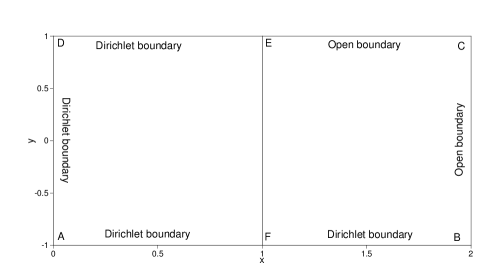
(a)

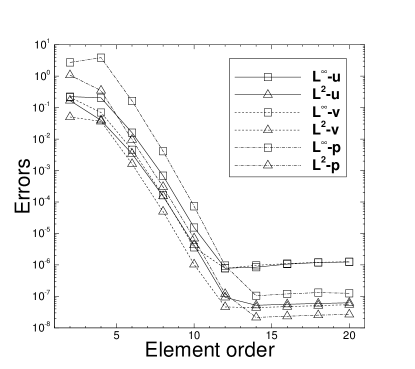
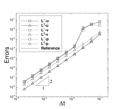
(b) (c)

Figure 1: Convergence tests (2D): (a) Mesh and configuration. $L^{\infty}$ and $L^{2}$ errors of the flow variables as a function of the element order with fixed $t_{f}=0.1$ and $\Delta t=0.001$ (b), and of the time step size $\Delta t$ with fixed element order $16$ and $t_{f}=0.5$ (c). OBC-C has been used on the open boundaries.

We consider the 2D rectangular domain $\overline{ABCD}$ shown in Figure 1(a), $0\leqslant x\leqslant 2$ and $-1\leqslant y\leqslant 1$, and the following analytic solution to the incompressible Navier-Stokes equations,

$$\left\{\begin{split}&u=2\cos(\pi y)\sin(\pi x)\sin t\\ &v=-2\sin(\pi y)\cos(\pi x)\sin t\\ &p=2\sin(\pi y)\sin(\pi x)\cos t\end{split}\right.$$ (87)

where $\mathbf{u}=(u,v)$. The external force $\mathbf{f}$ in (1a) is chosen such that the expressions in (87) satisfy (1a).

The domain is discretized using two uniform quadrilateral spectral elements ($\overline{AFED}$ and $\overline{FBCE}$) as shown in Figure 1(a). On the boundaries $\overline{AB}$, $\overline{AD}$ and $\overline{DE}$ Dirichlet boundary condition (73) is imposed, in which the boundary velocity $\mathbf{w}(\mathbf{x},t)$ is set according to the analytic expressions from (87). On the boundaries $\overline{BC}$ and $\overline{CE}$ the open boundary condition (95) (in Appendix B) is imposed, in which $\mathbf{f}_{b}$ is chosen such that the analytic expressions from (87) satisfy the equation (95) on $\partial\Omega_{o}$. The initial condition is given by (3), in which the initial velocity $\mathbf{u}_{in}$ is obtained according to the analytic solution in (87) by setting $t=0$.

The Navier-Stokes equations together with the open boundary conditions presented in Section 2.3 are solved using the numerical algorithm given in the Appendix B. The velocity and pressure fields are computed in time from $t=0$ to $t=t_{f}$ ($t_{f}$ to be specified later). Then the flow variables at $t=t_{f}$ from numerical simulations are compared with the analytic solutions in (87), and the numerical errors in various norms are computed. The element order and the time step size $\Delta t$ are varied systematically to study their effects on the numerical errors in spatial and temporal convergence tests, respectively. The non-dimensional viscosity in the Navier-Stokes equation (1a) is fixed at $\nu=0.01$ in the following tests.

Figure 1(b) demonstrates the results for the 2D spatial convergence tests. Here we have employed a fixed $t_{f}=0.1$ and $\Delta t=0.001$ (i.e. $100$ time steps) in the test. The element order is varied systematically between $2$ and $20$, and for each element order we have performed simulations and computed the errors of the numerical solutions at $t=t_{f}$ against the analytic solution. Figure 1(b) shows the numerical errors of the velocity and pressure in $L^{\infty}$ and $L^{2}$ norms as a function of the element order from this set of tests, in which OBC-C is employed on the open boundaries. It can be observed that the numerical errors decrease exponentially with increasing element order as the order is below $12$. For element orders $12$ and beyond, a saturation of the numerical errors can be observed at a level $10^{-7}\sim 10^{-6}$ due to the temporal truncation errors.

Figure 1(c) demonstrates the results for the 2D temporal convergence tests. Here we have employed a fixed $t_{f}=0.5$ and element order $16$. The time step size $\Delta t$ is varied systematically between $\Delta t=0.1$ and $\Delta t=1.953125e-4$. Figure 1(c) shows the $L^{\infty}$ and $L^{2}$ errors of the flow variables at $t=t_{f}$ as a function of $\Delta t$ in this group of tests. The open boundary condition is again OBC-C in these tests. The rate of convergence with respect to $\Delta t$ is observed to be second order when $\Delta t$ is sufficiently small.

Three Dimensions (3D)

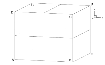
(a)

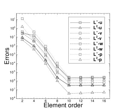
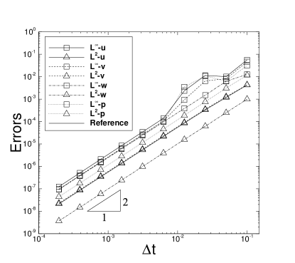
(b) (c)

Figure 2: Convergence tests (3D): (a) mesh of four hexahedral elements. $L^{\infty}$ and $L^{2}$ errors of the flow variables as a function of the element order with fixed $t_{f}=0.1$ and $\Delta t=0.001$ (b), and of the time step size $\Delta t$ with a fixed element order $12$ and $t_{f}=0.2$ (c). The faces $\overline{DCFG}$ and $\overline{BEFC}$ are open boundaries, on which the OBC-B is employed for the boundary condition.

We consider the 3D domain as sketched in Figure 2(a), $0.25\leqslant x\leqslant 1.25$, $-1\leqslant y\leqslant 1$, and $0\leqslant z\leqslant 2$, and the following analytic solutions to the Navier-Stokes equations on this domain,

$$\left\{\begin{split}&u=2\cos(2\pi x)\cos(\pi y)\cos(\pi z)\sin t\\ &v=2\sin(2\pi x)\sin(\pi y)\cos(\pi z)\sin t\\ &w=2\sin(2\pi x)\cos(\pi y)\sin(\pi z)\sin t\\ &p=2\sin(2\pi x)\sin(\pi y)\sin(\pi z)\cos t\end{split}\right.$$ (88)

where $\mathbf{u}=(u,v,w)$ in 3D. The external force $\mathbf{f}$ is chosen such that the analytic expressions in (88) satisfy the equation (1a). We assume that the domain and all the flow variables are periodic along the $z$ direction (on the faces $z=0$ and $z=2$). The faces $\overline{BEFC}$ and $\overline{DCFG}$ are open boundaries, on which the open boundary condition (74) will be imposed.

As discussed in Section 2.3, we employ a hybrid Fourier spectral method and spectral element method to discretize the 3D domain. Fourier spectral expansions are employed along the homogeneous $z$ direction, and spectral element expansions are employed in the $x$-$y$ planes. In the numerical tests that follow four Fourier planes are employed along the $z$ direction, and four quadrilateral elements are employed to discretize each plane. The boundary conditions (73) and (95) are imposed on the Dirichlet and open boundaries, in which the boundary velocity $\mathbf{w}$ is set in accordance with the analytic expressions (88) and the function $\mathbf{f}_{b}$ is chosen such that the analytic solutions in (88) satisfy (95) on the open boundaries. The algorithm from the Appendix B is employed to solve the incompressible Navier-Stokes equations, together with the Dirichlet and open boundary conditions. The flow fields are obtained from $t=0$ to $t=t_{f}$, and the errors of the numerical solution at $t=t_{f}$ are computed against the analytic solution given in (88). The non-dimensional viscosity is $\nu=0.01$ in the following tests.

In the spatial convergence tests, we fix the integration time at $t_{f}=0.1$ and the time step size at $\Delta t=0.001$, and then vary the element order systematically between $2$ and $16$. Figure 2(b) shows the numerical errors of the velocity and pressure at $t=t_{f}$ as a function of the element order, obtained using OBC-B for the open boundaries. An exponential decrease in the numerical errors can be observed when the element order is below $10$, and a saturation in the numerical errors is observed for element orders beyond $10$ due to the temporal truncation error.

In the temporal convergence tests we employ a fixed $t_{f}=0.2$ and an element order $12$, and then vary the time step size systematically between $\Delta t=0.1$ and $\Delta t=1.953125e-4$. We have computed the errors of the numerical solution at $t=t_{f}$ corresponding to each $\Delta t$ with OBC-B as the open boundary condition, and in Figure 2(c) these errors are plotted as a function of $\Delta t$ (in logarithmic scales) from these tests. The results signify a second-order rate of convergence in time.

To summarize, the 2D and 3D results of this section demonstrate that, with the open boundary conditions developed herein, the method exhibits a spatial exponential convergence rate and a temporal second-order accuracy for incompressible flows on domains with open/outflow boundaries.

3.2 Flow Past a Circular Cylinder

We focus on a canonical wake flow, the flow past a circular cylinder, in two and three dimensions in this section. At moderate and high Reynolds numbers, how to deal with the outflow boundary in this flow is critical to the stability of simulations. We employ this canonical problem to test the open/outflow boundary conditions developed in the current work.

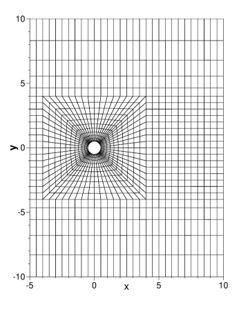
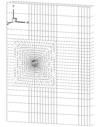
(a) (b)

Figure 3: Flow past a circular cylinder: spectral element meshes in (a) 2D, and (b) 3D. The 2D mesh and each $x$-$y$ plane of the 3D mesh contains $1228$ quadrilateral elements.

3.2.1 Two-Dimensional Simulations

Let us first investigate the cylinder flow numerically in two dimensions. Consider the domain in Figure 3(a), $-5\leqslant x/d\leqslant 10$ and $-10\leqslant y/d\leqslant 10$, where $d$ is the cylinder diameter. The center of the cylinder coincides with the origin of the coordinate system. The top and bottom of the domain ($y=\pm 10d$) are assumed to be periodic. A uniform flow (free-stream velocity $U_{0}$, along the $x$ direction) enters the domain from the left side, and the wake exits the domain through the right boundary at $x=10d$. We assume that no external body force is present, and thus $\mathbf{f}=0$ in equation (1a). In the following simulations all the length variables are normalized based on the cylinder diameter $d$, and all the velocity variables are normalized by the free stream velocity $U_{0}$. So the Reynolds number is defined based on $U_{0}$ and $d$. All the other variables are normalized accordingly in a consistent way.

We discretize the domain using the spectral element mesh shown in Figure 3(a), which contains $1228$ quadrilateral elements. The algorithm from the Appendix B is used to numerically solve the incompressible Navier-Stokes equations together with the boundary conditions specified as follows. On the cylinder surface no-slip condition is imposed, i.e. the Dirichlet boundary condition (73) with $\mathbf{w}=0$. At the inlet ($x/d=-5$) we impose the Dirichlet condition (73) where the boundary velocity $\mathbf{w}$ is set based on the free-stream velocity. Periodic conditions are imposed at the top and bottom of the domain for all flow variables. At the outflow boundary ($x/d=10$) the boundary condition (74) from Section 2.3 is imposed, where OBC-A, OBC-B and OBC-C are all employed and the various algorithmic parameters have been tested.

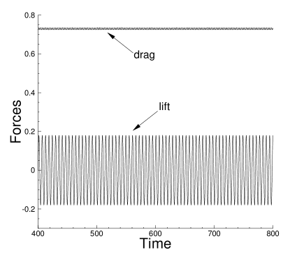
Figure 4: Time histories of drag ($x$ component of force, $f_{x}$) and lift ($y$ component of force, $f_{y}$) on the cylinder at $Re=100$, computed using an element order $8$ and OBC-B as the outflow boundary condition in 2D.

$Re$	element order	mean-$f_{x}$	rms-$f_{x}$	rms-$f_{y}$
$30$	$4$	$0.968$	$0$	$0$
	$6$	$0.968$	$0$	$0$
	$8$	$0.968$	$0$	$0$
	$10$	$0.968$	$0$	$0$
$100$	$4$	$0.729$	$0.00374$	$0.126$
	$6$	$0.730$	$0.00377$	$0.127$
	$8$	$0.730$	$0.00377$	$0.127$
	$10$	$0.730$	$0.00377$	$0.127$

Table 1: Flow past a cylinder (2D): forces on the cylinder computed using several element orders. OBC-B is used for the outflow boundary condition.

Figure 4 illustrates a long-time simulation of the 2D cylinder flow at Reynolds number $Re=100$ with a window of time histories of the forces (drag $f_{x}$, and lift $f_{y}$) acting on the cylinder obtained from current simulations. The results are obtained using an element order $8$ and OBC-B as the outflow boundary condition. Periodic vortex shedding into the wake induces a fluctuating drag and lift force exerting on the cylinder. Based on these histories we can compute the statistical quantities such as the time-averaged mean and root-mean-square (rms) forces. Table 1 lists the mean and rms forces on the cylinder at Reynolds numbers $Re=30$ and $100$ obtained using several element orders ranging from $4$ to $10$. The mean lift is not shown in the table because they are all zeros at $Re=30$ and all essentially zeros at $Re=100$. Note that the flow is in a steady state at $Re=30$, and so no averaging is performed with the forces at this Reynolds number. When the element order is sufficiently large ($6$ or above), the forces obtained from the simulations are essentially the same, suggesting convergence of the simulation results with respect to the grid resolution. The majority of simulations in subsequent discussions are performed using an element order $8$ and a time step size $\Delta t=2.5e-4$, and at lower Reynolds numbers (below $Re=60$) an element order $6$ and $\Delta t=1e-3$ have also been employed. A range of Reynolds numbers (to be specified below) has been simulated and studied for this problem.

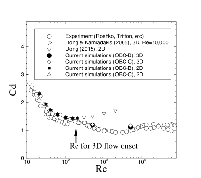
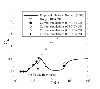
(a) (b)

Figure 5: Flow past a cylinder: Comparison of the drag coefficient (a) and the rms lift coefficient (b) as a function of the Reynolds number between current simulations (2D/3D) and the experimental measurements. OBC-B and OBC-C are used as the outflow boundary condition with current simulations.

We first study this flow for a range of low Reynolds numbers ($Re=200$ and below). The physical flow is two-dimensional and is either at a steady state (for $Re\lesssim 45$) or unsteady with periodic vortex shedding (for $Re\lesssim 185$) Williamson1996 . We have conducted simulations at several Reynolds numbers in this range, and computed the corresponding forces on the cylinder. Figures 5(a) and (b) are comparisons of the drag coefficients ($C_{d}$) and rms lift coefficients ($C_{L}$) obtained from current simulations with those from the experimental measurements and simulations from the literature Wieselsberger1921 ; Finn1953 ; Tritton1959 ; Roshko1961 ; Norberg2003 ; DongKER2006 ; Dong2015obc . These coefficients are defined by

$$C_{d}=\frac{\bar{f}_{x}}{\frac{1}{2}\rho_{f}U_{0}^{2}},\quad C_{L}=\frac{f_{y}^{\prime}}{\frac{1}{2}\rho_{f}U_{0}^{2}}$$ (89)

where $\bar{f}_{x}$ denotes the time-averaged (mean) drag, $f_{y}^{\prime}$ denotes the rms-lift on the cylinder, and $\rho_{f}$ is the fluid density. Note that the plots also include results from the three-dimensional simulations, which will be discussed subsequently in Section 3.2.2. The current 2D results are obtained using the OBC-B and OBC-C as the outflow boundary conditions. We observe that in this range of the Reynolds numbers the current 2D simulation results are in good agreement with the experimental data, and they also agree well with the results from Dong2015obc . When the Reynolds number is beyond this range (above $Re\approx 185\sim 260$), the physical flow will undergo a transition and become three-dimensional Williamson1996 . So there will be a large discrepancy between the drag/lift coefficients from 2D simulations and the experimentally observed values DongK2005 ; DongS2015 ; Dong2015obc .

$Re$	method	parameters	mean-$f_{x}$	rms-$f_{x}$	rms-$f_{y}$
10	OBC-A	$a_{11}=a_{22}=$ 0.95	1.652	0	0
		0.9	1.652	0	0
		0.5	1.648	0	0
		0.2	1.644	0	0
		0.1	1.641	0	0
		0.0	1.639	0	0
		-0.1	1.635	0	0
		-0.2	1.630	0	0
		-0.5	1.593	0	0
		-0.9	1.445	0	0
		-0.95	1.427	0	0
	OBC-B		1.631	0	0
	OBC-C		1.631	0	0
	Traction-free OBC		1.631	0	0
20	OBC-A	$a_{11}=a_{22}=$ 0.95	1.173	0	0
		0.9	1.173	0	0
		0.5	1.171	0	0
		0.2	1.168	0	0
		0.1	1.166	0	0
		0.0	1.164	0	0
		-0.1	1.162	0	0
		-0.2	1.158	0	0
		-0.5	1.121	0	0
		-0.9	0.967	0	0
		-0.95	0.952	0	0
	OBC-B		1.159	0	0
	OBC-C		1.159	0	0
	Traction-free OBC		1.159	0	0
100	OBC-A	$a_{11}=a_{22}=$ 0.95	0.734	0.00412	0.128
		0.9	0.734	0.00412	0.127
		0.5	0.732	0.00392	0.125
		0.2	0.731	0.00378	0.126
		0.1	0.731	0.00377	0.126
		0.0	0.731	0.00377	0.126
		-0.1	0.730	0.00378	0.127
		-0.2	0.730	0.00382	0.127
		-0.5	0.723	0.00425	0.131
		-0.9	(unstable)
		-0.95	(unstable)
	OBC-B		0.730	0.00377	0.127
	OBC-C		0.730	0.00378	0.127
	Traction-free OBC		0.729	0.00381	0.127

Table 2: 2D cylinder flow: comparison of the mean and rms forces on the cylinder obtained using OBC-A (with $\alpha=1/2$ and various parameters $a_{11}=a_{22}$), OBC-B, and OBC-C for several Reynolds numbers. Results from the traction-free open boundary condition are included as a reference.

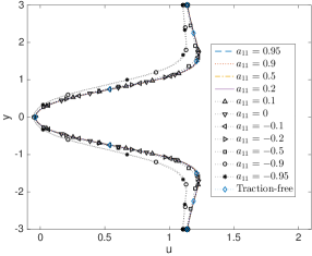
(a) at $x=1.0$

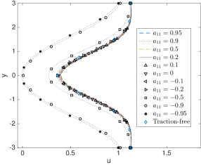
(b) at $x=5.0$

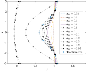
(c) at $x=10.0$ (outlet)

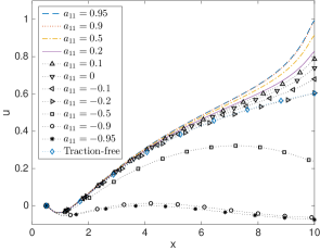
(d) along centerline $y=0$

Figure 6: Cylinder flow ($Re=20$): comparison of streamwise velocity (i.e. $x$ velocity component) profiles at several downstream locations in the wake and along the centerline computed using OBC-A with $\alpha=1/2$ and different $a_{11}$ (and $a_{22}$, with $a_{22}=a_{11}$) values. Results from traction-free condition are included for comparison.

At these low Reynolds numbers it is relatively easy to carry out a study of how the algorithmic parameters affect the simulation results. OBC-A, OBC-B and OBC-C have all been employed and tested with the open boundary condition (74) in current simulations.

Let us first concentrate on OBC-A. In Table 2 we list the (time-averaged) mean and rms forces on the cylinder at three Reynolds numbers ($Re=10$, $20$ and $100$), obtained using OBC-A as the outflow boundary condition under a range of values for $a_{11}$ (and $a_{22}$, with $a_{22}=a_{11}$) and with a fixed $\alpha=\frac{1}{2}$. Since the flow is steady at $Re=10$ and $20$, no time-averaging is performed for these two Reynolds numbers. As a reference for comparison, we have also included the results computed using the traction-free condition on the outflow boundary, namely,

$$-p\mathbf{n}+\nu\mathbf{n}\cdot\nabla\mathbf{u}=0,\quad\text{on}\ \partial\Omega_{o}.$$ (90)

A trend can be discerned from the data obtained using OBC-A. The mean drag on the cylinder computed using OBC-A tends to decrease with decreasing $a_{11}$ (and $a_{22}$) values. When compared with the results based on the traction-free condition, the best results with OBC-A seem to correspond to a value around $a_{11}=a_{22}\approx-0.2$ for the cylinder flow. In an interval around this best value, the computed forces seem to be not sensitive to $a_{11}$ ($a_{22}$) and they are very close to the forces corresponding to the traction-free condition. Even when $a_{11}=a_{22}=0.95$, the discrepancy in the mean drag seems to be around $1\%$. But as $a_{11}=a_{22}\rightarrow-1$, the discrepancy in the mean drag seems to grow rapidly and becomes very substantial. For example, with $a_{11}=a_{22}=-0.95$ the difference in the mean drag values produced by OBC-A and the traction-free condition is approximately $18\%$ at $Re=20$. In addition, we observe that at $Re=100$, with $a_{11}=a_{22}=-0.9$ and smaller, the computation with OBC-A is unstable. We recall that as $a_{11}=a_{22}\rightarrow 1$ the amount of dissipation on $\partial\Omega_{o}$ with OBC-A becomes infinite, and as $a_{11}=a_{22}\rightarrow-1$ the amount of dissipation approaches zero. The above results with the computed forces suggest that, while the best $a_{11}$ ($a_{22}$) values seem to be around $-0.2$, larger values appear not harmful, but it can be detrimental to the accuracy if $a_{11}$ ($a_{22}$) is too small.

The velocity distribution in the cylinder wake demonstrates the effects of $a_{11}$ (and $a_{22}$) on the simulation results even more clearly. Figure 6 is a comparison of the steady-state streamwise velocity ($x$ velocity) profiles along the vertical direction at downstream locations $x/d=1.0$, $5.0$ and $10.0$ (plots (a), (b) and (c)), and along the centerline (plot (d)). The different curves correspond to OBC-A as the outflow boundary condition with $\alpha=\frac{1}{2}$ and a set of $a_{11}$ (and $a_{22}$, with $a_{22}=a_{11}$) values ranging from $-0.95$ to $0.95$. For the purpose of comparison, the velocity profiles computed using the traction-free condition (90) are also included in these plots. We have the following observations:

• The velocity profiles corresponding to OBC-A with $a_{11}=a_{22}=-0.5$ and below exhibit a large discrepancy when compared with the rest of the profiles in essentially the entire wake region.

• The profiles corresponding to OBC-A with $a_{11}=a_{22}=-0.2$ and above are quite close to those resulting from the traction-free boundary condition (90) in the near wake ($x/d\lesssim 5$). Further downstream ($x/d\gtrsim 6$) the discrepancy in all the profiles (except the one with $a_{11}=a_{22}=-0.2$), when compared with the traction-free condition, becomes very pronounced.

• Among the set of $a_{11}$ ($a_{22}$) values tested for OBC-A, the best profile corresponds to $a_{11}=a_{22}=-0.2$, in terms of the comparison with results based on the traction-free condition.

The effects of the $a_{11}$ and $a_{22}$ parameters in OBC-A on the simulation results are investigated with a fixed $\alpha=\frac{1}{2}$ in the above. Studies of the $a_{11}$ ($a_{22}$) effect with other $\alpha$ values are also performed, but not as systematically. The above observed behaviors of OBC-A with respect to $a_{11}$ and $a_{22}$ appear to also apply to other $\alpha$ values.

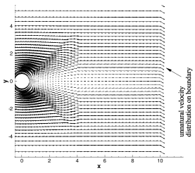
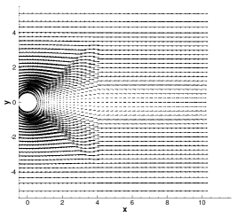
(a) (b) (c)

Figure 7: 2D Cylinder flow ($Re=20$): velocity fields computed using OBC-A ($\alpha=0$, $a_{11}=a_{22}=a_{12}=0$) with different $a_{21}$ values: (a) $a_{21}=-0.4$, (b) $a_{21}=0.4$, and (c) $a_{21}=0$. Un-physical velocity distributions can be observed at the outflow boundary if $a_{21}\neq 0$ with OBC-A. Velocity vectors are plotted on every eighth quadrature points in each direction within each element.

With OBC-A, when $\alpha=0$, the $\mathbf{R}$ matrix may not be diagonal in 2D, as long as its elements $a_{ij}$ ($i,j=1,2$) satisfy the conditions (47a), (47b) and (50). We observe however that non-zero off-diagonal elements ($a_{21}$ and $a_{12}$), especially when $a_{21}\neq 0$, can result in poor or unphysical simulation results with OBC-A. This point is demonstrated by the velocity distributions (steady-state) in Figure 7 for Reynolds number $Re=20$, which are computed using OBC-A with $\alpha=0$ and several $a_{21}$ values ($a_{21}=-0.4$, $0.0$ and $0.4$), while $a_{11}=a_{22}=a_{12}=0$ in the $\mathbf{R}$ matrix. At this Reynolds number the velocity is expected to be approximately in the horizontal direction at the outflow boundary. To one’s surprise, when $a_{21}\neq 0$, the computed velocity at the outflow boundary points to an oblique direction, even though all the velocity vectors are approximately along the horizontal direction inside the domain; see Figures 7(a)-(b). The angle of the velocity vectors on the boundary depends on the sign and the magnitude of $a_{21}$. If $a_{21}=0$, on the other hand, the computed velocity is approximately along the horizontal direction as expected (Figure 7(c)). The above unphysical results can be understood by considering equation (52b) for OBC-A, which in this case is reduced to the following on the boundary,

$$\nu\frac{\partial v}{\partial x}=\frac{\lambda_{1}-\lambda_{3}}{\mathscr{K}}a_{21}u+\frac{\lambda_{1}}{\mathscr{K}}v$$ (91)

where $u$ and $v$ are the $x$ and $y$ components of the velocity. This equation indicates that the horizontal velocity $u$ will contribute to the vertical velocity $v$ at the outflow boundary when $a_{21}\neq 0$. Therefore, even if $v=0$ inside the domain, a non-zero $v$ will be generated on the outflow boundary due to the boundary condition, leading to poor velocity distributions. By considering equation (52a), one can infer that the parameter $a_{12}$ has an analogous effect. It induces a contribution of the tangent velocity $u_{\tau}$ to the normal velocity $u_{n}$ on the open boundary. In practical simulations, $a_{12}$ seems not as detrimental to the results as $a_{21}$ does, which is probably because of the pressure term involved in $T_{nn}$ in equation (52a).

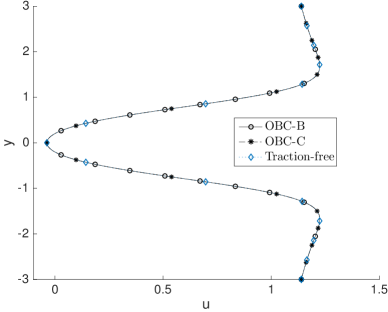
(a) at $x=1.0$

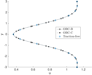
(b) at $x=5.0$

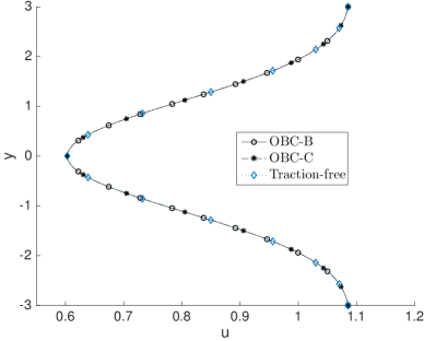
(c) at $x=10.0$ (outlet)

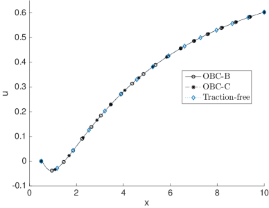
(d) along centerline $y=0$

Figure 8: 2D Cylinder flow ($Re=20$): Streamwise velocity profiles at several downstream locations in the wake and along the centerline of domain, computed using OBC-B and OBC-C as the outflow boundary condition. Velocity profiles obtained with the traction-free condition are included for comparison.

Let us next consider OBC-B and OBC-C. Table 2 also lists the mean and rms forces on the cylinder at the Reynolds numbers $Re=10$, $20$ and $100$ that are computed using OBC-B and OBC-C as the outflow boundary condition. It is observed that the computed forces based on OBC-B and OBC-C are identical to those based on the traction-free condition for $Re=10$ and $20$. For $Re=100$, the forces obtained using OBC-B and OBC-C are essentially the same as that from the traction-free condition, with only a negligible difference.

Figure 8 shows a comparison of the streamwise velocity profiles along the vertical direction at three downstream locations ($x/d=1.0$, $5.0$ and $10.0$) and along the centerline ($y/d=0$) among results computed using OBC-B, OBC-C, and the traction-free condition at Reynolds number $Re=20$. Note that $x/d=10$ is the outflow boundary in this problem. We observe that all the velocity profiles computed using OBC-B and OBC-C and the traction-free condition exactly overlap with one another. These results suggest that both OBC-B and OBC-C result in the same flow distributions as the traction-free condition.

Let us next consider the cylinder flow at higher Reynolds numbers ($Re\geqslant 2000$). At these Reynolds numbers the vortices shed from the cylinder can persist far downstream into the wake, and thus may cross the outflow boundary and exit the domain. This can cause severe difficulties and instabilities (backflow instability DongKC2014 ) to conventional methods. Energy-stable boundary conditions are critical to overcoming the backflow instability for successful simulations at these Reynolds numbers. We have conducted long-time simulations at several Reynolds numbers ranging from $Re=2000$ to $Re=10000$ using the methods developed herein to test their performance. Note that the traction-free boundary condition is unstable for simulations in this range of these Reynolds numbers.

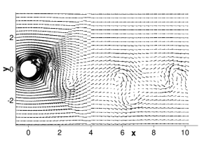
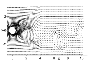
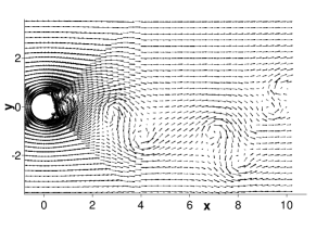
(a) (b) (c)

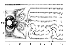
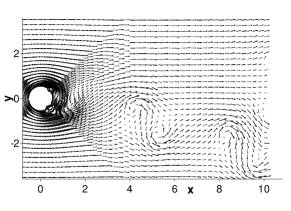
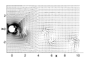
(d) (e) (f)

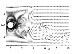
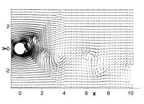
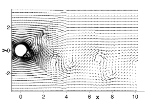
(g) (h) (i)

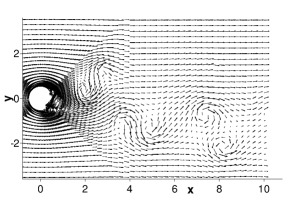
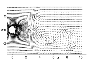
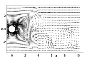
(j) (k) (l)

Figure 9: Temporal sequence of snapshots of velocity fields ($Re=5000$): (a) $t=443.2$, (b) $t=444.2$, (c) $t=445.2$, (d) $t=446.2$, (e) $t=447.2$, (f) $t=448.2$, (g) $t=449.2$, (h) $t=450.2$, (i) $t=451.2$, (j) $t=452.2$, (k) $t=453.2$, (l) $t=454.2$. Velocity vectors are plotted on every eighth quadrature points in each direction within each element. Results are obtained using OBC-B as the outflow boundary condition.

Figure 9 shows a temporal sequence of snapshots of the instantaneous velocity fields at $Re=5000$, illustrating the dynamics of the cylinder wake based on two-dimensional simulations. These results are obtained using OBC-B as the outflow boundary condition, and the element order is $8$ and $\Delta t=2.5e-4$ in the simulations. One can observe pairs of vortices shed from the cylinder. These vortices are convected downstream and persist in the entire wake region. The vortices successively approach and pass through the outflow boundary, and discharge from the domain. It is observed that our method is able to allow the vortices to cross the outflow/open boundary and exit the domain in a fairly natural way (see Figures 9(a)-(e) and 9(f)-(i)). But some distortion to the vortices can also be observed as they pass through the outflow boundary.

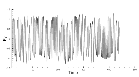
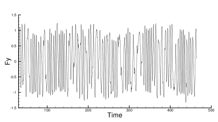
(a) (b)

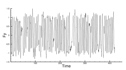
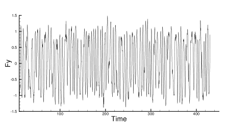
(c) (d)

Figure 10: Time histories of the lift on the cylinder at Reynolds numbers $Re=5000$ ((a) and (b)) and $Re=10000$ ((c) and (d)). Results in (a) and (c) are computed using OBC-B, and those in (b) and (d) are computed using OBC-C, as the outflow boundary condition.

Long-time simulations have been performed and our methods are stable for these high Reynolds numbers. The long-term stability of the method is demonstrated by Figure 10, which plots the time histories of the lift on the cylinder at Reynolds numbers $Re=5000$ (Figure 10(a)-(b)) and $Re=10000$ (Figure 10(c)-(d)). These simulations are conducted using OBC-B (Figure 10(a) and (c)) and OBC-C (Figure 10(b) and (d)) as the outflow boundary condition. The long-term stability of the simulations and the chaotic nature of flow are evident from the time signals.

3.2.2 Three-Dimensional Simulations

We next look into the simulation of the cylinder flow in three dimensions. Consider the 3D domain sketched in Figure 3(b), $-5d\leqslant x\leqslant 10d$, $-10d\leqslant y\leqslant 10d$, and $0\leqslant z\leqslant L_{z}$, where $d$ again denotes the cylinder diameter and $L_{z}$ is the domain dimension along the $z$ direction. The cylinder axis is assumed to coincide with the $z$ axis of the coordinate system. The top and bottom of domain ($y=\pm 10d$) are assumed to be periodic. We also assume that all the flow variables and the domain are homogeneous along the $z$ direction and are periodic at $z=0$ and $z=L_{z}$, and therefore a Fourier expansion of the field variables in $z$ can be carried out. A uniform inflow with a free stream velocity $U_{0}$ enters the domain at $x=-5d$ along the $x$ direction, and the wake discharges from the domain through the boundary at $x=10d$. As in 2D simulations, all length variables are normalized by the cylinder diameter $d$ and all velocity variables are normalized by the free stream velocity $U_{0}$. Therefore, the Reynolds number is defined based on $U_{0}$ and $d$.

We consider two Reynolds numbers $Re=500$ and $5000$ for 3D simulations in this paper. We employ a domain dimension $L_{z}/d=1.0$ along the $z$ direction for $Re=500$ and a dimension $L_{z}/d=2.0$ for $Re=5000$. The domain is discretized using $32$ uniform points (i.e. $32$ Fourier planes) along the $z$ direction, and each of the plane ($x$-$y$ plane) is discretized using a mesh of $1228$ quadrilateral spectral elements with an element order $6$. Figure 3(b) is a sketch of the 3D domain and the spectral element mesh within the $x$-$y$ planes. In the current work the mesh used in each $x$-$y$ plane for the 3D simulations is exactly the same as that of Figure 3(a) for the 2D simulations in Section 3.2.1. We impose the no-slip condition (i.e. zero velocity) on the cylinder surface, and the Dirichlet condition (73) on the left boundary ($x=-5d$), in which the boundary velocity is set according to the free stream velocity. On the top/bottom boundaries ($y=\pm 10d$) periodic boundary conditions are imposed. Along the $z$ direction a periodic condition is enforced because of the Fourier expansions of the field variables. On the outflow boundary $x=10d$ the open boundary condition (74) from Section 2 is imposed. Both OBC-B and OBC-C are employed for 3D simulations. Long-time simulations are performed and the flow has reached a statistically stationary state. So the initial conditions will have no effect on the state of the flow. The normalized time step size is $\Delta t=2.5e-4$ in the simulations.

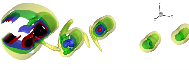
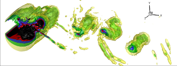
(a) (b)

Figure 11: (color online) Visualization of vortices in 3D cylinder flow: Pressure isosurfaces (five uniform levels between $p=-0.6$ and $p=-0.2$) at Reynolds numbers (a) $Re=500$ and (b) $Re=5000$. Results are obtained with OBC-C as the outflow boundary condition.

Figure 11 shows a visualization of the vortices in the cylinder wake by plotting the iso-surfaces of the pressure fields at $Re=500$ (plot (a)) and $Re=5000$ (plot (b)). These results are obtained using OBC-C as the outflow boundary condition. In addition to the spanwise vortices (“rollers”) in the wake, 3D flow structures along the streamwise direction can be clearly observed. With the larger Reynolds number, the flow structures exhibit notably finer length scales, and the flow field is much noisier.

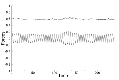
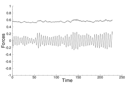
(a) (b)

Figure 12: 3D cylinder flow: time histories of drag and lift on the cylinder at Reynolds numbers (a) $Re=500$ and (b) $Re=5000$. Results correspond to OBC-B as the outflow boundary condition.

Figure 12 shows the time histories of the drag and lift on the cylinder at the two Reynolds numbers $Re=500$ (plot (a)) and $Re=5000$ (plot (b)) from the 3D simulations, which are obtained using OBC-B as the outflow boundary condition. The history signals show that the flow has reached a statistically stationary state. They also demonstrate the long-term stability of the methods developed herein. The energy-stable boundary conditions are critical to the stability of 3D simulations at moderate and high Reynolds numbers. It is observed that with the traction-free outflow boundary condition the 3D simulation is unstable at the higher Reynolds number $Re=5000$. One can also compare the lift history in Figure 12(b) from 3D simulations with that in Figure 10(a) from 2D simulations, both at Reynolds number $Re=5000$ and corresponding to OBC-B as the outflow boundary condition. It can be observed that the 2D simulation leads to much larger lift amplitudes (and correspondingly larger rms lift coefficient) than the 3D simulation for the same Reynolds number, which is well-known in the literature DongK2005 ; DongKER2006 .

We have computed the drag coefficient and the rms lift coefficient based on the force histories at $Re=500$ and $Re=5000$. These data from 3D simulations are included in Figure 5 for comparison with the experimentally determined coefficient values. It is observed that the current 3D simulation results are in reasonably good agreement with the values from the experimental measurements. In contrast, 2D simulations grossly over-predict both the drag and the rms-lift coefficients in the regime where the flow is physically three-dimensional.

3.3 Jet Impinging on a Wall

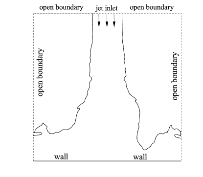
Figure 13: Problem configuration of the impinging jet on a wall.

In this section we test further the current methods with another flow problem, a jet impinging on a solid wall, using two-dimensional simulations. Due to the open boundaries and the physical instability of the jet, the open boundary condition is critical to the successful simulation of this flow.

Specifically, we study a fluid jet of diameter $d$ impinging on a wall in two dimensions. Figure 13 illustrates the configuration of this problem. Consider a rectangular domain, $-\frac{5}{2}d\leqslant x\leqslant\frac{5}{2}d$ and $0\leqslant y\leqslant 5d$, where $x$ and $y$ axes are along the horizontal and vertical directions, respectively. The bottom side of the domain is a solid wall. The inlet of the jet (with diameter $d$) is located in the middle of the top side of the domain, namely, $-R_{0}\leqslant x\leqslant R_{0}$ and $y=5d$, where $R_{0}$ is the radius of the inlet ($R_{0}=\frac{d}{2}$). The jet velocity is assumed to have the following profile at the inlet,

$$\left\{\begin{split}&u=0\\ &v=-U_{0}\left[\tanh\frac{1-x/R_{0}}{\sqrt{2}\epsilon/d}\left(H(x,0)-H(x,R_{0})\right)+\tanh\frac{1+x/R_{0}}{\sqrt{2}\epsilon/d}\left(H(x,-R_{0})-H(x,0)\right)\right]\end{split}\right.$$ (92)

where $U_{0}$ is the velocity scale ($U_{0}=1$), $\epsilon=\frac{1}{40}d$, and $H(x,a)$ is the unit step function, taking the unit value if $x\geqslant a$ and vanishing otherwise. The rest of the domain boundaries, on the top and on the left and right sides, are all open, where the fluid can freely enter or leave the domain. The jet enters the domain through the inlet on the top, impinges on the bottom wall and splits into two streams, which then flow sideways out of the domain. The goal is to simulate and study this process.

We discretize the domain using a spectral element mesh of $400$ quadrilateral elements, with $20$ uniform elements along the $x$ and $y$ directions. No-slip condition (i.e. Dirichlet condition with zero velocity) is imposed on the bottom wall. At the jet inlet we impose the Dirichlet condition (73), in which the boundary velocity $\mathbf{w}$ is given by (92). On the rest of the domain boundary the open boundary condition (74) is imposed, and the three boundary conditions (OBC-A, OBC-B and OBC-C) are employed and tested. Long-time simulations have been performed, and the flow has reached a statistically stationary state. So the initial condition is immaterial and will have no effect on the long-term behavior of the flow. The problem and the physical variables are normalized based on the jet diameter $d$ and the velocity scale $U_{0}$ in the simulations. So the Reynolds number is defined based on these scales accordingly. In accordance with the previous simulations of a variant of this problem DongS2015 , we employ an element order $12$ and a time step size $\Delta t=2.5e-4$ for the current simulations.

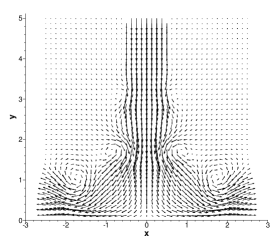
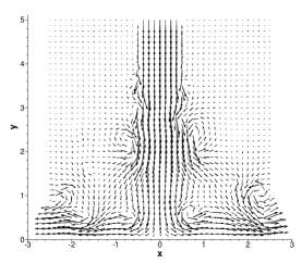
(a) (b) (c)

Figure 14: Characteristics of the impinging jet: instantaneous velocity distribution at Reynolds numbers (a) $Re=300$, (b) $Re=2000$, and (c) $Re=10000$. Velocity vectors are plotted on every eighth quadrature point in each direction within each element. Results are computed using OBC-C as the open boundary condition.

An overview of the characteristics of this flow is provided by Figure 14. This figure shows the instantaneous velocity fields at three Reynolds numbers: $Re=300$, $2000$ and $10000$, which are computed using OBC-C as the open boundary condition. At a sufficiently low Reynolds number (e.g. $Re=300$) this flow is at a steady state. After impinging on the wall, the vertical jet splits into two horizontal streams, and flow in opposite directions parallel to the wall until they exit the domain (Figure 14(a)). In regions of the domain outside the jet stream the velocity appears to be negligibly small. As the Reynolds number increases the flow becomes unsteady. The vertical jet stream appears to be stable within some distance downstream of the inlet, and then the Kelvin-Helmholtz instability develops and the jet becomes physically unstable. Successive pairs of vortices form along the profile of the jet, and they are convected downstream and eventually out of the domain along with the jet (Figure 14(b)). For even higher Reynolds numbers, the region downstream of the inlet with a stable jet profile shrinks, and the onset of instability moves markedly upstream toward the inlet. The vortices forming along the jet profile appear more irregular and numerous, and their interactions lead to more complicated dynamics (Figure 14(c)).

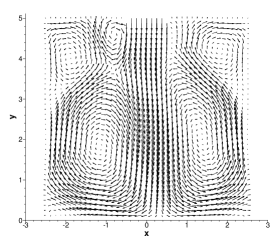
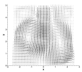
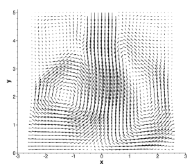
(a) (b) (c)

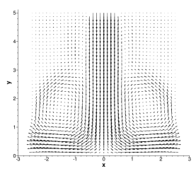
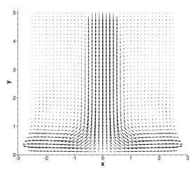
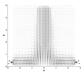
(d) (e) (f)

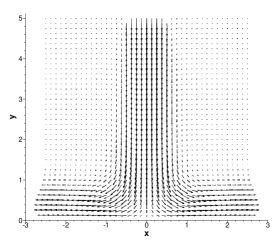
(g) (h)

Figure 15: Impinging jet ($Re=300$): velocity field distributions computed using OBC-A with $\alpha=\frac{1}{2}$ ((a)-(f)), the traction-free condition (g), and OBC-B (h). Different parameter values for $a_{11}$ (and $a_{22}$, with $a_{22}=a_{11}$) have been tested with OBC-A. They are $a_{11}=a_{22}=0.5$ (a), $0.2$ (b), $0.0$ (c), $-0.2$ (d), $-0.5$ (e), and $-0.75$ (f). Velocity vectors are plotted on every eighth quadrature points in each direction within each element.

method	parameters	$f_{y}$ (or mean-$f_{y}$)	rms-$f_{y}$
OBC-A	$a_{11}=a_{22}=-0.75$	$-0.912$	0
	$-0.5$	$-0.986$	0
	$-0.2$	$-1.189$	0
	$0$	$-1.384$	$0.0408$
	$0.2$	$-1.653$	$0.102$
	$0.5$	$-2.343$	$0.0922$
OBC-B		$-0.994$	0
OBC-C		$-0.994$	0
Traction-free OBC		$-1.026$	0

Table 3: Impinging jet ($Re=300$): vertical force on the wall computed using OBC-A (with $\alpha=1/2$ and various $a_{11}=a_{22}$ values), OBC-B, OBC-C, and the traction-free condition.

Let us first focus on a low Reynolds number $Re=300$ and study the effects of different open boundary conditions on the simulation results. Figure 15 is a comparison of the velocity field distributions at $Re=300$ computed using OBC-A with $\alpha=\frac{1}{2}$ and a range of values for $a_{11}$ (and $a_{22}$, with $a_{22}=a_{11}$). The result obtained using the traction-free open boundary condition (90) and OBC-B are also included for comparison. The results in this figure can be compared with that of Figure 14(a), which is also for $Re=300$ but computed using OBC-C as the open boundary condition. We can make the following observations from these results:

• OBC-B and OBC-C result in velocity field distributions similar to the traction-free condition.

• The $a_{11}$ (and $a_{22}$) values strongly influence the velocity fields computed with OBC-A. The velocity distributions obtained using OBC-A with different $a_{11}$ (and $a_{22}$) values are qualitatively different.

• The velocity distributions obtained using OBC-A with $a_{11}=a_{22}=0.5$, $0.2$, $0$, and $-0.2$ exhibit a pair (or more) of large vortices filling up the domain, which is unphysical. With the larger $a_{11}$ (and $a_{22}$) values, the velocity fields even indicate that the flow and the vortices go out of the domain through the upper open boundary.

• The flow fields obtained using OBC-A with $a_{11}=a_{22}=0.5$, $0.2$ and $0$ are not a steady flow for this Reynolds number. The forces on the wall obtained with these methods fluctuate over time, albeit in a narrow range.

• The velocity distributions computed using OBC-A with $a_{11}=a_{22}=-0.5$ and $-0.75$ exhibit a similarity to that obtained with the traction-free condition in the overall characteristics. However, in the horizontal jet streams obtained with these methods, the directions of the velocity vectors seem un-natural at the open boundary (Figure 15(e)-(f)). In addition, although it appears quite weak, a pair of large vortices can be discerned from the velocity field obtained using OBC-A with $a_{11}=a_{22}=-0.5$ (Figure 15(e)).

• Using the velocity field resulting from the traction-free condition as a reference, the best result for OBC-A seems to correspond to a parameter value around $a_{11}=a_{22}=-0.5$ for this problem.

Table 3 lists the forces ($y$-component) on the wall obtained using different methods at $Re=300$. Since the flow computed using OBC-A with $a_{11}=a_{22}=0.5$, $0.2$ and $0.0$ is unsteady, listed in the table are the mean and rms forces corresponding to these methods. We observe that with increasing $a_{11}$ (and $a_{22}$), the force computed using OBC-A increases substantially in magnitude. The discrepancy in the forces between OBC-A and the traction-free condition is significant. Compared with the traction-free condition, the best result obtained using OBC-A appears to correspond to a value around $a_{11}=a_{22}=-0.5$. On the other hand, the forces obtained using OBC-B and OBC-C are the same, and they are very close to the that obtained using the traction-free condition.

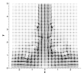
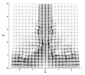
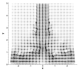
(a) (b) (c)

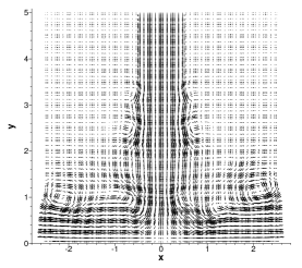
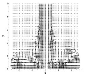
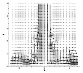
(d) (e) (f)

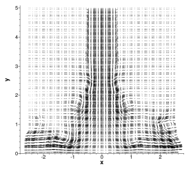
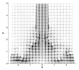
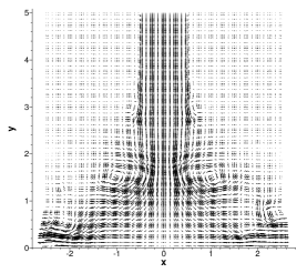
(g) (h) (i)

Figure 16: Impinging jet ($Re=5000$): temporal sequence of snapshots of the instantaneous velocity fields at (a) $t=619.05$, (b) $t=619.65$, (c) $t=620.25$, (d) $t=620.85$, (e) $t=621.45$, (f) $t=622.05$, (g) $t=622.65$, (h) $t=623.25$, (i) $t=623.85$. Velocity vectors are plotted on every fourth quadrature point in each direction within each element. Results are computed using OBC-B as the open boundary condition.

Let us next look into the impinging jet at higher Reynolds numbers. Figure 16 shows a temporal sequence of snapshots of the velocity fields at $Re=5000$ computed using OBC-B as the open boundary condition. These results illustrate the vortex-pair formation and the transport of the train of vortices downstream along the jet profile in the dynamics of the flow. They also signify that the method herein can allow the vortices to pass through the open boundary in a smooth and fairly natural fashion; see the left boundary in Figures 16(c)-(f). On the other hand, a certain degree of distortion to the vortices as they cross the open boundary can also be observed (Figure 16(f)). The physical instability of the jet and the presence of vortices on the open boundaries make these simulations very challenging. The current open boundary conditions are very effective for such problems. It is noted that the traction-free condition is unstable in these simulations.

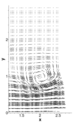
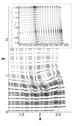
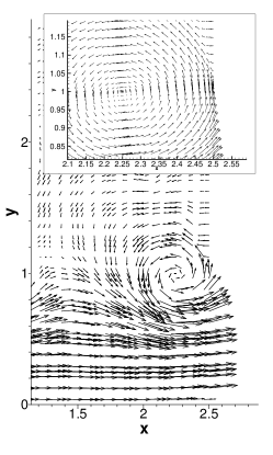
(a) (b) (c)

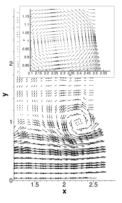
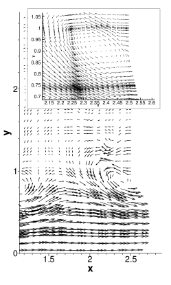
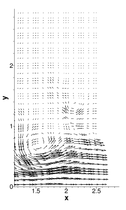
(d) (e) (f)

Figure 17: Impinging jet ($Re=5000$): a temporal sequence of snapshots of the velocity fields near the right open boundary showing the discharge of a vortex from the domain, computed using OBC-C as the open boundary condition. (a) $t=593.4$, (b) $t=593.7$, (c) $t=594$. (d) $t=594.3$, (e) $t=594.6$. (f) $t=595.5$. Velocity vectors are plotted on every fourth quadrature points in each direction within each element. The insets of plots (b)–(e) show a blow-up view of the velocity vectors (shown on every quadrature point) near the boundary.

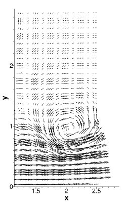
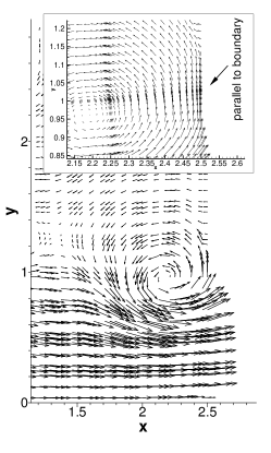
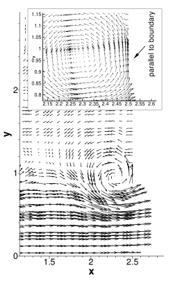
(a) (b) (c)

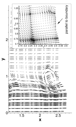
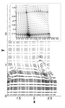
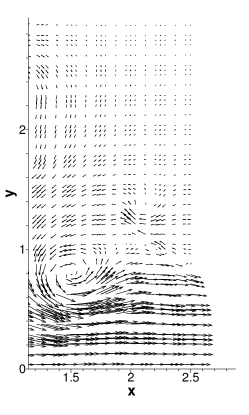
(d) (e) (f)

Figure 18: Impinging jet ($Re=5000$): a temporal sequence of snapshots of the velocity fields near the right open boundary showing the discharge of a vortex from the domain, computed using the open boundary condition from Dong2015obc (without the inertia term). (a) $t=1137.75$, (b) $t=1138.05$, (c) $t=1138.35$. (d) $t=1138.65$, (e) $t=1138.95$. (f) $t=1139.85$. Velocity vectors are plotted on every fourth quadrature points in each direction within each element. The insets of plots (b)–(e) show a blow-up view of the velocity vectors (shown on every quadrature point) near the boundary.

Let us next take a closer view of the distortion to the vortices as they exit the domain through the open boundary. Figure 17 illustrates the typical scenario when a vortex crosses the open boundary, obtained with the current open boundary condition OBC-C. This figure shows a temporal sequence of velocity fields near the right open boundary and the bottom wall. The insets of Figures 17(b)–(e) are magnified views of a section of the open boundary near the vortex core. As the vortex approaches the open boundary, the velocity patterns show that the vortex maintains an almost perfect circular shape, with essentially no or very little distortion (Figure 17(a)-(d)). Then as the vortex core moves very close to the boundary a notable deformation to the vortex becomes evident (Figure 17(e)). The vortex deforms into an oval and is elongated in an oblique direction to the boundary. The vortex retains an oval shape until it discharges completely from the domain. For comparison, Figure 18 shows a comparable and typical scenario of the vortex exiting the domain obtained using the open boundary condition from Dong2015obc , but without the inertia (i.e. time derivative) term therein so that the boundary condition is also a traction-type condition. We observe a similar process, with the initial circular vortex distorted into an oval shape as it moves out of the domain (Figure 18(e)). But the velocity patterns of Figures 17 and 18 also reveal a notable difference. The vortex in Figure 18 experiences another type of distortion, even before the distortion into an oval becomes evident. More specifically, we observe that, as the vortex approaches the open boundary, on the section of the boundary influenced by the vortex rotation and in its vicinity, the velocity vectors tend to point along the tangential direction to the boundary. This is evident from the insets of Figures 18(b)-(d). This makes the velocity pattern in that region less congruent or incongruent with those outside the region, thus causing an apparent distortion to the vortex. This is especially evident from Figures 18(c) and (d). As the vortex further evolves in time, this distortion seems to disappear and gives way to the distortion into an oval vortex (Figures 18(d)-(e)). By contrast, from the velocity patterns obtained using the current open boundary condition we observe that the vortex retains an essentially perfect shape (see Figures 17(b)-(d)) and does not experience such a distortion as evidenced from Figure 18, before the oval deformation kicks in. These results suggest that the current open boundary conditions can be more favorable compared with that of Dong2015obc in the sense that they can produce more congruent and more natural velocity distributions near/at the open boundary and cause less distortion to the vortices as they pass through the boundary and exit the domain.

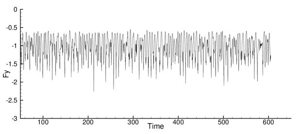
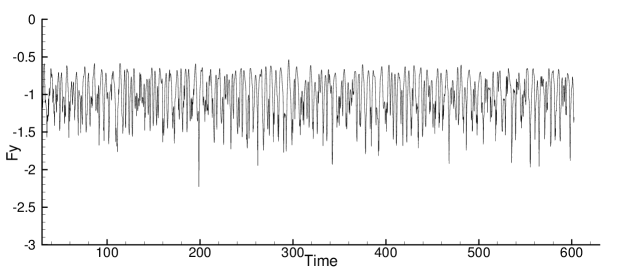
(a) (a)

Figure 19: Impinging jet: time histories of the vertical force on the bottom wall at $Re=10000$ computed using OBC-B (a) and OBC-C (b) as the open boundary condition.

Long-time simulations have been performed using the current methods for the impinging jet flow. Figure 19 illustrates the time histories of the vertical force on the wall at $Re=10000$, which are obtained using OBC-B and OBC-C as the open boundary condition, respectively. The long history signals demonstrate the long-term stability of the methods developed in the current work, and that the flow has reached a statistically stationary state.

4 Concluding Remarks

In this paper we have developed a set of new energy-stable open boundary conditions for simulating outflow/open-boundary problems of incompressible flows. These boundary conditions can effectively overcome the backflow instability, and give rise to stable and accurate simulation results when strong vortices or backflows occur at the open/outflow boundary.

The development of these boundary conditions involves two steps. First, we devise a general form of the boundary conditions that ensure the energy stability on the open boundary by reformulating the boundary contribution into a quadratic form involving a symmetric matrix. Second, we require that the scale of the boundary dissipation, upon imposing the boundary conditions from the previous step, should match a physical scale and thus attain the final boundary conditions.

Both of these two steps are crucial. The first step ensures energy stability, and the second step ensures physical correctness and accuracy. Those boundary conditions resulting from the first step only are referred to as “OBC-A” in the current paper, and the boundary conditions “OBC-B” and “OBC-C” studied in the current paper involve both steps in the development. Extensive numerical experiments have been conducted to test the accuracy and performance of these boundary conditions. These tests show that, as expected, all three conditions (OBC-A, OBC-B and OBC-C) produce stable simulations, even when strong vortices or backflows occur at the open/outflow boundary. However, it is observed that OBC-A in general gives rise to poor or even unphysical simulation results, unless the algorithmic parameters take some “optimal” value for the flow problem under study. It is further observed that the “optimal” parameter values for OBC-A are unfortunately flow-problem dependent. For example, for the cylinder flow the “optimal” values for $a_{11}$ ($a_{22}$) are around $a_{11}=a_{22}=-0.2$, while for the impinging jet problem they are around $a_{11}=a_{22}=-0.5$ with OBC-A. It is further noted that OBC-A gives rise to poor simulation results with $a_{11}=a_{22}=-0.5$ for the cylinder flow and with $a_{11}=a_{22}=-0.2$ for the impinging jet problem. These observations suggest that OBC-A, i.e. the energy-stable boundary conditions resulting from the first step only, may only be of limited use in practice. While OBC-A leads to stable computations, the simulation results in general can deviate from the physical results considerably. In contrast, the open boundary conditions OBC-B and OBC-C lead to favorable results in terms of both stability and accuracy. Numerical experiments show that they produce stable and accurate simulation results, in terms of comparisons with both the experimental measurements and the results produced by other methods.

The open boundary conditions devised based on the quadratic form and the eigen problem of the symmetric matrix involved therein can be formulated into a traction-type condition; see equation (74). It is noted that the boundary conditions herein in general give rise to a non-zero traction on the entire open boundary, in both the backflow regions (if any) and the normal outflow regions. This is in contrast to the energy-stable boundary conditions in previous works in the literature (see e.g. DongS2015 ), which results in a non-zero traction in the backflow regions only and a zero traction in the normal outflow regions of the open boundary.

While their formulations are different, numerical experiments indicate that OBC-B and OBC-C tend to produce very similar or the same simulation results. The various numerical experiments appear to give a sense that the fluctuations in the physical quantities (e.g. forces) produced by OBC-B can at times be somewhat larger than that by OBC-C, resulting in e.g. higher values in the largest amplitude in the time-history signals. In such a sense, OBC-C may be somewhat more favorable when compared with OBC-B. But the difference in their simulation results, if any, is minor.

While the current open boundary conditions can allow the vortices to cross the open/outflow boundary and exit the domain in a smooth and fairly natural fashion, even at quite high Reynolds numbers, a certain level of distortion to the vortices is also evident during the process. For example, an otherwise circular vortex can deform into an oval while exiting the domain through the open boundary. This type of distortion is also observed with previous methods (see e.g. Dong2015obc ). However, as shown by the results in Section 3.3, the current open boundary condition seems more favorable compared with that of Dong2015obc (without the inertia term) in terms of the distortions, because the current condition leads to velocity distributions more congruent on the open boundary and in its vicinity. In contrast, the boundary condition of Dong2015obc can lead to less congruent or incongruent velocity distributions on sections of the open boundary where the vortices cross, causing additional distortions to the vortices.

It should be pointed out that, since the current open boundary conditions are formulated in a traction form, it is not difficult to extend these conditions to arrive at a set of corresponding “convective-like” energy-stable open boundary conditions, by e.g. incorporating an appropriate inertia term in a similar way to Dong2015obc . This may be desirable in term of the control over the velocity field on the open/outflow boundaries.

Backflow instability is one of the primary issues encountered when scaling up the Reynolds number in the simulations of a large class of incompressible flows, such as wakes, jets, shear layers, and cardiovascular and respiratory flows. The method developed in the current work provides a new effective technique to algorithmically eliminate the backflow instability. Algorithmic elimination of the backflow instability can be critical to and will be instrumental in flow simulations at high (and moderate) Reynolds numbers. For example, it enables one to employ a significantly smaller computational domain (permitted by accuracy consideration), thus leading to a much higher spatial resolution than otherwise, even with the same mesh size. The current work contributes a useful and effective tool toward the numerical simulations of such challenging problems.

Appendix A. Proof of Theorem 2.1

Since $\mathbf{A}$ and $\mathbf{G}$ are symmetric and real matrices, all their eigenvalues are real. None of the eigenvalues of $\mathbf{A}$ is zero because $\text{det}(\mathbf{A})\neq 0$. Suppose $\lambda$ ($\lambda\neq 0$) is an eigenvalue of $\mathbf{A}$. Then

$$\begin{split}0&=\text{det}\begin{bmatrix}-\lambda\mathbf{I}&-\mathbf{I}\\ -\mathbf{I}&\mathbf{G}-\lambda\mathbf{I}\end{bmatrix}=\text{det}(-\lambda\mathbf{I})\text{det}\left[(\mathbf{G}-\lambda\mathbf{I})-(-\mathbf{I})(-\lambda\mathbf{I})^{-1}(-\mathbf{I})\right]\\ &=(-\lambda)^{m}\text{det}\left[\mathbf{G}-\left(\lambda-\frac{1}{\lambda}\right)\mathbf{I}\right]\\ &\Longrightarrow\quad\text{det}\left[\mathbf{G}-\left(\lambda-\frac{1}{\lambda}\right)\mathbf{I}\right]=0,\end{split}$$ (93)

where we have used the Schur complement. Therefore $\left(\lambda-\frac{1}{\lambda}\right)$ is an eigenvalue of $\mathbf{G}$. Suppose $\xi$ is an eigenvalue of $\mathbf{G}$, and $\lambda-\frac{1}{\lambda}=\xi$. Then $\lambda=\frac{\xi}{2}\pm\sqrt{\left(\frac{\xi}{2}\right)^{2}+1}\neq 0.$ So the steps in equation (93) can be reversed. We conclude that $\lambda$ is an eigenvalue of the matrix $\mathbf{A}$.

Suppose $\begin{bmatrix}\mathbf{Z}\\ -\lambda\mathbf{Z}\end{bmatrix}$ is an eigenvector of $\mathbf{A}$ corresponding to the eigenvalue $\lambda$. Then $\mathbf{Z}\neq 0$ and

$$\begin{split}0&=\begin{bmatrix}-\lambda\mathbf{I}&-\mathbf{I}\\ -\mathbf{I}&\mathbf{G}-\lambda\mathbf{I}\end{bmatrix}\begin{bmatrix}\mathbf{Z}\\ -\lambda\mathbf{Z}\end{bmatrix}=\begin{bmatrix}0\\ -\mathbf{Z}-\lambda(\mathbf{G}-\lambda\mathbf{I})\mathbf{Z}\end{bmatrix}=\begin{bmatrix}0\\ -\lambda\left(\mathbf{G}-\left(\lambda-\frac{1}{\lambda}\right)\mathbf{I}\right)\mathbf{Z}\end{bmatrix}\\ &\Longrightarrow\quad\left(\mathbf{G}-\left(\lambda-\frac{1}{\lambda}\right)\mathbf{I}\right)\mathbf{Z}=0.\end{split}$$ (94)

We conclude that $\mathbf{Z}$ is an eigenvector of $\mathbf{G}$ corresponding to the eigenvalue $(\lambda-\frac{1}{\lambda})$. Now suppose $(\lambda-\frac{1}{\lambda})$ is an eigenvalue of $\mathbf{G}$ and $\mathbf{Z}$ is the corresponding eigenvector. Then $\lambda\neq 0$, and the steps in (94) can be reversed. So we conclude that $\begin{bmatrix}\mathbf{Z}\\ -\lambda\mathbf{Z}\end{bmatrix}$ is an eigenvector of $\mathbf{A}$ corresponding to the eigenvalue $\lambda$.

Appendix B. Numerical Algorithm

In this appendix we provide a summary of our algorithm for numerically solving the equations (1a)–(1b), together with the boundary conditions (73) and (74). This algorithm is based on the scheme originally developed in Dong2015obc (presented in Section 2.4 of Dong2015obc ).

We modify the outflow/open boundary condition (74) slightly by adding a source term as follows,

$$-p\mathbf{n}+\nu\mathbf{n}\cdot\nabla\mathbf{u}-\mathbf{E}(\mathbf{u},\partial\Omega_{o})=\mathbf{f}_{b}(\mathbf{x},t),\quad\text{on}\ \partial\Omega_{o}$$ (95)

where $\mathbf{f}_{b}$ is a prescribed source term on $\partial\Omega_{o}$ for the purpose of numerical testing only, and it will be set to $\mathbf{f}_{b}=0$ in actual simulations. $\mathbf{E}(\mathbf{u},\partial\Omega_{o})$ is given by either (75).

The following algorithm is for equations (1a)–(1b), together with the boundary conditions (73) on $\partial\Omega_{d}$ and (95) on $\partial\Omega_{o}$. Let $n\geqslant 0$ denote the time step index, and $(\cdot)^{n}$ denote the variable $(\cdot)$ at time step $n$. Let $J$ ($J=1$ or $2$) denote the temporal order of accuracy of the scheme. Given $\mathbf{u}^{n}$, we compute $(p^{n+1},\mathbf{u}^{n+1})$ successively in a de-coupled manner in two steps:
For $p^{n+1}$:

$$\frac{\gamma_{0}\tilde{\mathbf{u}}^{n+1}-\hat{\mathbf{u}}}{\Delta t}+\mathbf{u}^{*,n+1}\cdot\nabla\mathbf{u}^{*,n+1}+\nabla p^{n+1}+\nu\nabla\times\nabla\times\mathbf{u}^{*,n+1}=\mathbf{f}^{n+1}$$ (96a)

$$\nabla\cdot\tilde{\mathbf{u}}^{n+1}=0$$ (96b)

$$\mathbf{n}\cdot\tilde{\mathbf{u}}^{n+1}=\mathbf{n}\cdot\mathbf{w}^{n+1},\quad\text{on}\ \partial\Omega_{d}$$ (96c)

$$p^{n+1}=\nu\mathbf{n}\cdot\nabla\mathbf{u}^{*,n+1}\cdot\mathbf{n}-\mathbf{n}\cdot\mathbf{E}(\mathbf{u}^{*,n+1},\partial\Omega_{o})-\mathbf{f}_{b}^{n+1}\cdot\mathbf{n},\quad\text{on}\ \partial\Omega_{o}.$$ (96d)

For $\mathbf{u}^{n+1}$:

$$\frac{\gamma_{0}\mathbf{u}^{n+1}-\gamma_{0}\tilde{\mathbf{u}}^{n+1}}{\Delta t}-\nu\nabla^{2}\mathbf{u}^{n+1}=\nu\nabla\times\nabla\times\mathbf{u}^{*,n+1}$$ (97a)

$$\mathbf{u}^{n+1}=\mathbf{w}^{n+1},\quad\text{on}\ \partial\Omega_{d}$$ (97b)

$$\mathbf{n}\cdot\nabla\mathbf{u}^{n+1}=\frac{1}{\nu}\left[p^{n+1}\mathbf{n}+\mathbf{E}(\mathbf{u}^{*,n+1},\partial\Omega_{o})-\nu\left(\nabla\cdot\mathbf{u}^{*,n+1}\right)\mathbf{n}+\mathbf{f}_{b}^{n+1}\right],\quad\text{on}\ \partial\Omega_{o}.$$ (97c)

In the above equations, $\Delta t$ is the time step size, $\mathbf{n}$ is the outward-pointing unit vector normal to the boundary, and $\tilde{\mathbf{u}}^{n+1}$ is an auxiliary variable approximating $\mathbf{u}^{n+1}$. $\mathbf{u}^{*,n+1}$ is a $J$-th order explicit approximation of $\mathbf{u}^{n+1}$ given by

$$\mathbf{u}^{*,n+1}=\left\{\begin{array}[]{ll}\mathbf{u}^{n},&J=1,\\ 2\mathbf{u}^{n}-\mathbf{u}^{n-1},&J=2.\end{array}\right.$$ (98)

$\hat{\mathbf{u}}$ and the constant $\gamma_{0}$ are such that the expressions $\frac{1}{\Delta t}(\gamma_{0}\mathbf{u}^{n+1}-\hat{\mathbf{u}})$ and $\frac{1}{\Delta t}(\gamma_{0}\tilde{\mathbf{u}}^{n+1}-\hat{\mathbf{u}})$ approximate $\left.\frac{\partial\mathbf{u}}{\partial t}\right|^{n+1}$ with a $J$-th order backward differentiation formula, and they are given by

$$\hat{\mathbf{u}}=\left\{\begin{array}[]{ll}\mathbf{u}^{n},&J=1,\\ 2\mathbf{u}^{n}-\frac{1}{2}\mathbf{u}^{n-1},&J=2,\end{array}\right.\qquad\quad\gamma_{0}=\left\{\begin{array}[]{ll}1,&J=1,\\ \frac{3}{2},&J=2.\end{array}\right.$$ (99)

By taking the $L^{2}$ inner products between a test function and equation (96a), one can obtain the weak form about $p^{n+1}$. By taking the $L^{2}$ between a test function and the equation obtained by summing up equations (96a) and (97a), one can get the weak form about $\mathbf{u}^{n+1}$. Let $H_{p0}^{1}(\Omega)=\left\{\ v\in H^{1}(\Omega)\ :\ v|_{\partial\Omega_{o}}=0\ \right\},$ and $H_{u0}^{1}(\Omega)=\left\{\ v\in H^{1}(\Omega)\ :\ v|_{\partial\Omega_{d}}=0\ \right\}.$ Let $q\in H_{p0}^{1}(\Omega)$ and $\varphi\in H_{u0}^{1}(\Omega)$ denote the test functions for the pressure and velocity. Then the weak form for $p^{n+1}$ is

$$\begin{split}\int_{\Omega}\nabla p^{n+1}\cdot\nabla q=&\int_{\Omega}\mathbf{G}^{n+1}\cdot\nabla q-\nu\int_{\partial\Omega_{d}\cup\partial\Omega_{o}}\mathbf{n}\times\bm{\omega}^{*,n+1}\cdot\nabla q-\frac{\gamma_{0}}{\Delta t}\int_{\partial\Omega_{d}}\mathbf{n}\cdot\mathbf{w}^{n+1}q,\ \forall q\in H_{p0}^{1}(\Omega),\end{split}$$ (100)

where $\bm{\omega}^{*,n+1}=\nabla\times\mathbf{u}^{*,n+1}$, and

$$\mathbf{G}^{n+1}=\mathbf{f}^{n+1}+\frac{\hat{\mathbf{u}}}{\Delta t}-\mathbf{u}^{*,n+1}\cdot\nabla\mathbf{u}^{*,n+1}.$$ (101)

The weak form for $\mathbf{u}^{n+1}$ is

$$\begin{split}\frac{\gamma_{0}}{\nu\Delta t}\int_{\Omega}\mathbf{u}^{n+1}\varphi&+\int_{\Omega}\nabla\varphi\cdot\nabla\mathbf{u}^{n+1}=\frac{1}{\nu}\int_{\Omega}\left(\mathbf{G}^{n+1}-\nabla p^{n+1}\right)\varphi\\ &+\frac{1}{\nu}\int_{\partial\Omega_{o}}\left[p^{n+1}\mathbf{n}+\mathbf{E}(\mathbf{u}^{*,n+1},\partial\Omega_{o})+\mathbf{f}_{b}^{n+1}-\nu\left(\nabla\cdot\mathbf{u}^{*,n+1}\right)\mathbf{n}\right]\varphi,\quad\forall\varphi\in H_{u0}^{1}(\Omega).\end{split}$$ (102)

The weak forms (100) and (102) can be discretized in space using a high-order spectral element method Dong2015obc or a combined spectral-element and Fourier-spectral method DongK2005 ; Dong2007 .

Given $\mathbf{u}^{n}$, the following operations are involved in the final algorithm within a time step for computing $p^{n+1}$ and $\mathbf{u}^{n+1}$:

• Solve equation (100), together with the Dirichlet condition (96d) on $\partial\Omega_{o}$, for $p^{n+1}$.

• Solve equation (102), together with the Dirichlet condition (97b) on $\partial\Omega_{d}$, for $\mathbf{u}^{n+1}$.

References

- [1] Y. Bazilevs, J.R. Hohean, T.J.R. Hughes, R.D. Moser, and Y. Zhang. Patient-specific isogeometric fluid-structure interaction analysis of theracic aortic blood flow due to impantation of the jarvik 2000 left ventricular assist device. Comput. Methods Appl. Mech. Engrg., 198:3534–3550, 2009.
- [2] C. Bertoglio and A. Caiazzo. A tangential regularization method for backflow stabilization in hemodynamics. Journal of Computational Physics, 261:162–171, 2014.
- [3] C. Bertoglio and A. Caiazzo. A stokes-residual backflow stabilization method applied to physiological flows. Journal of Computational Physics, 313:260–278, 2016.
- [4] C. Bertoglio, A. Caiazzo, Y. Bazilevs, M. Braack, M. Esmaily, V. Gravemeier, A.L. Marsden, O. Pironeau, I.E. Vignon-Clementel, and W.A. Wall. Benchmark problems for numerical treatment of backflow at open boundaries. International Journal for Numerical Methods in Biomedical Engineering, 34:e2918, 2018.
- [5] M. Braack and P.B. Mucha. Directional do-nothing condition for the navier-stokes equations. Journal of Computational Mathematics, 32:507–521, 2014.
- [6] C.-H. Bruneau and P. Fabrie. Effective downstream boundary conditions for incompressible Navier-Stokes equations. International Journal for Numerical Methods in Fluids, 19:693–705, 1994.
- [7] C.-H. Bruneau and P. Fabrie. New efficient boundary conditions for incompressible navier-stokes equations: a well-posedness result. Mathematical Modeling and Numerical Analysis, 30:815–840, 1996.
- [8] S. Dong. Direct numerical simulation of turbulent Taylor-Couette flow. J. Fluid Mech., 587:373–393, 2007.
- [9] S. Dong. An outflow boundary condition and algorithm for incompressible two-phase flows with phase field approach. Journal of Computational Physics, 266:47–73, 2014.
- [10] S. Dong. A convective-like energy-stable open boundary condition for simulations of incompressible flows. Journal of Computational Physics, 302:300–328, 2015.
- [11] S. Dong and G.E. Karniadakis. DNS of flow past stationary and oscillating cylinder at . J. Fluids Struct., 20:14–23, 2005.
- [12] S. Dong, G.E. Karniadakis, and C. Chryssostomidis. A robust and accurate outflow boundary condition for incompressible flow simulations on severely-truncated unbounded domains. Journal of Computational Physics, 261:83–105, 2014.
- [13] S. Dong, G.E. Karniadakis, A. Ekmekci, and D. Rockwell. A combined DNS-PIV study of the turbulent near wake. J. Fluid Mech., 569:185–207, 2006.
- [14] S. Dong and J. Shen. A pressure-correction scheme for generalized form of energy-stable open boundary conditions for incompressible flows. Journal of Computational Physics, 291:254–278, 2015.
- [15] S. Dong and X. Wang. A rotational pressure-correction scheme for incompressible two-phase flows with open boundaries. PLoS One, 11(5):e0154565, 2016.
- [16] M. Feistauer and T. Neustupa. On the existence of a weak solution of viscous incompressible flow past a cascade of profiles with an arbitrarily large inflow. J. Math. Fluid Mech., 15:701–715, 2013.
- [17] R.K. Finn. Determination of the drag on a cylinder at low Reynolds numbers. Journal of Applied Physics, 24:771–773, 1953.
- [18] J. Fouchet-Incaux. Artifical boundaries and formulations for the incompressible navier-stokes equations. applications to air and blood flows. SeMA Journal, 64:1–40, 2014.
- [19] N.S. Ghaisas, D.A. Shetty, and S.H. Frankel. Large eddy simulation of turbulent horizontal buoyant jets. Journal of Turbulence, 16:772–808, 2015.
- [20] V. Gravemeier, A. Comerford, L. Yoshihara, M. Ismail, and W.A. Wall. A novel formulation for Neumann inflow boundary conditions in biomechanics. International Journal for Numeical Methods in Biomedical Engineering, 28:560–573, 2012.
- [21] P.M. Gresho. Incompressible fluid dynamics: some fundamental formulation issues. Annual Review of Fluid Mechanics, 23:413–453, 1991.
- [22] J.G. Heywood, R. Rannacher, and S. Turek. Artificial boundaries and flux and pressure: conditions for the incompressible navier-stokes equations. International Journal for Numerical Methods in Fluids, 22:325–352, 1996.
- [23] M. Ismail, V. Gravemeier, A. Comerford, and W.A. Wall. A stable approach for coupling multidimensional cardiovascular and pulmonary networks based on a novel pressure-flow rate or pressure-only neumann boundary condition formulation. International Journal for Numerical Methods in Biomedical Engineering, 30:447–469, 2014.
- [24] G.E. Karniadakis and S.J. Sherwin. Spectral/hp element methods for computational fluid dynamics, 2nd edn. Oxford University Press, 2005.
- [25] M. Lanzendorfer and J. Stebel. On perssure boundary conditions for steady flows of incompressible fluids with pressure and shear rate dependent viscosities. Applications of Mathematics, 56:265–285, 2011.
- [26] M.E. Moghadam, Y. Bazilevs, T.-Y. Hsia, I.E. Vignon-Clementel, and A.L. Marsden. A comparison of outlet boundary treatments for prevention of backflow divergence with relevance to blood flow simulations. Comput. Mech., 48:277–291, 2011.
- [27] C. Norberg. Fluctuating lift on a circular cylinder: review and new measurements. Journal of Fluids and Structures, 17:57–96, 2003.
- [28] J. Nordstrom. A roadmap to well posed and stable problems in computational physics. Journal of Scientific Computing, 71:365–385, 2017.
- [29] J. Nordstrom and C.L. Cognata. Energy-stable boundary conditions for the incompressible navier-stokes equations. Mathematics of Computation, in press, 2018.
- [30] A. Porpora, P. Zunino, C. Vergara, and M. Piccinelli. Numerical treatment of boundary conditions to replace branches in hemodynamics. International Journal of Numerical Methods in Biomedical Engineering, 28:1165–1183, 2012.
- [31] A. Roshko. Experiments on the flow past a circular cylinder at very high Reynolds numbers. Journal of Fluid Mechanics, 10:345–356, 1961.
- [32] R.L. Sani and P.M. Gresho. Resume and remarks on the open boundary conidtion minisymposium. International Journal for Numerical Methods in Fluids, 18:983–1008, 1994.
- [33] S.J. Sherwin and G.E. Karniadakis. A triangular spectral element method: applications to the incompressible navier-stokes equations. Comput. Meth. Appl. Mech. Engrg., 123:189–229, 1995.
- [34] D.J. Tritton. Experiments on the flow past a circular cylinder at low Reynolds numbers. Journal of Fluid Mechanics, 6:547, 1959.
- [35] S.S. Varghese, S.H. Frankel, and P.F. Fischer. Direct numerical simulation of stenotic flows. Part 1. steday flow. Journal of Fluid Mechanics, 582:253–280, 2007.
- [36] C. Wieselsberger. Recent statements on the laws of liquid and air resistancy. Physikalische Zeitschrift, 22:321–328, 1921.
- [37] C.H.K. Williamson. Vortex dynamics in a cylinder wake. Annual Review of Fluid Dynamics, 28:477–539, 1996.
- [38] Z. Yang and S. Dong. Multiphase flows of N immiscible incompressible fluids: an outflow boundary condition and algorithm. Journal of Computational Physics, 366:33–70, 2018.
- [39] X. Zheng and S. Dong. An eigen-based high-order expansion basis for structured spectral elements. Journal of Computational Physics, 230:8573–8602, 2011.