Design and Analysis of Efficient Maximum/Minimum Circuits for Stochastic Computing
Abstract
In stochastic computing (SC), a real-valued number is represented by a stochastic bit stream, encoding its value in the probability of obtaining a one. This leads to a significantly lower hardware effort for various functions and provides a higher tolerance to errors (e.g., bit flips) compared to binary radix representation. The implementation of a stochastic max/min function is important for many areas where SC has been successfully applied, such as image processing or machine learning (e.g., max pooling in neural networks). In this work, we propose a novel shift-register-based architecture for a stochastic max/min function. We show that the proposed circuit has a significantly higher accuracy than state-of-the-art architectures at comparable hardware cost. Moreover, we analytically proof the correctness of the proposed circuit and provide a new error analysis, based on the individual bits of the stochastic streams. Interestingly, the analysis reveals that for a certain practical bit stream length a finite optimal shift register length exists and it allows to determine the optimal length.
Index Terms:
Stochastic computing, sequential logic, finite state machine, stochastic max/min functionI Introduction
Sochastic computing (SC) is a promising computing paradigm, which represents a real-valued number by a stochastic stream [1, 2, 3]. The value is encoded by the probability of obtaining a one in the stream. Compared to binary radix representation, the stochastic representation leads to low hardware cost and high fault tolerance to circuit noise and bit flips [4, 5].
In SC, basic arithmetic operations can be realized with simple combinational logic [1]. Moreover, combinational logic can be synthesized to implement arbitrary polynomial functions, by manipulating them into a Bernstein polynomial with coefficients in the unit interval [6, 7, 8]. However, in order to implement more complex (non-linear) functions, sequential logic is required [9, 4]. In particular, linear finite-state machines (FSM) have been proposed to implement complex functions, which can be realized by either employing saturating up/down counters or shift registers [10]. The stochastic exponentiation and the tanh function were presented in [9] and the absolute value as well as exponentiation based on an absolute value were proposed in [4]. Recently, a new synthesis method which allows to implement arbitrary functions using FSM-based elements was introduced in [11].
In recent years, SC has been successfully applied to a variety of applications such as decoding of modern error correcting codes [12, 13, 14], control systems [15, 16], image processing [17, 18, 19], filter design [20, 21], and neural networks [22, 23, 9, 24]. Most of these applications exploit the low complexity circuitry of SC in algorithms that do not require a high numerical precision of the final result.
In many of the aforementioned application domains, the efficient implementation of a stochastic max/min (SMax/SMin) function is very important. Especially, for neural networks, where such functions are the key element in the max pooling layer [22, 23]. Two architectures for SMax functions111Both circuits can be easily converted to realize a SMin function. have been proposed in literature [17, 23]. The implementation in [17] is based on a stochastic comparator, which requires a stochastic number generator (SNG) that is usually realized by a linear feedback shift register. In order to reduce the overhead of the SNG, an optimized SMax function was proposed in [23]. However, both approaches have only been validated empirically.
Thus, the first goal of this paper is to analytically prove the correctness of the SMax functions in [17, 23]. Then, we propose a novel shift-register-based architecture for a stochastic SMax/SMin function and analytically prove its correctness. We show that the novel architecture provides a higher accuracy than [17, 23] at comparable hardware cost. We provide a new error analysis of the proposed circuit, considering the individual bits of the stochastic streams. To the best of our knowledge, no such analysis has been done before for an FSM-based stochastic computing element. Based on the error analysis we show that for practical bit stream lengths a finite optimal shift register length exists. Moreover, we determine the optimal shift register size for certain bit stream lengths.
II Stochastic Computing Basics
In this section, we briefly review the main principles of SC and introduce the basic computing elements used in this work. A comprehensive overview on SC can be found in [2] and recent challenges and potential solutions are discussed in [3].
II-A Unipolar Coding Format
In the unipolar coding format222It is important to note that the circuits proposed in this work are also valid for the bipolar format, which enables the representation of negative values [1]., the value of a deterministic number is encoded in a stochastic bit stream of length . The individual bits in the stochastic stream are indicated by . The probability for each bit in the stream to be one is given by . In practical realizations, the rate of ones in the stochastic bit stream is used to represent the number
| (1) |
where denotes the number of ones in the stream. The precision (representation resolution) of the unipolar format is given by . Thus, only if , otherwise is only an approximation of .
II-B Combinational Logic-based SC Elements
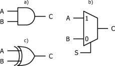
Certain arithmetic operations in SC can be implemented by single combinational elements, for example scaled addition and multiplication can be realized using a multiplexer and an AND gate, respectively. Moreover, an XOR gate with the input streams and implements the function , which involves addition and subtraction. In the following, we briefly explain the principles of the aforementioned operations, as they are the main building blocks of the SMax/SMin functions presented in Secs. III and IV.
II-B1 Multiplication
The stochastic multiplication can be implemented using a simple AND gate as shown in Fig. 1a. If we assume that the input stochastic streams and are uncorrelated and have the probabilities and , then we have at the output
| (2) |
For the unipolar format the values encoded by the stochastic streams , and are , and , and, thus we obtain
| (3) |
II-B2 Scaled Addition
The stochastic circuit for scaled addition, a multiplexer, is shown in Fig. 1b. If we assume that the stochastic streams and are uncorrelated with the stochastic stream , and , and are their corresponding probabilities, the output can be expressed as
| (4) |
According to the unipolar format, we substitute , , and by , , and , and obtain the following output
| (5) |
In order to perform unbiased addition, is set to .
II-B3 Non-Scaled Addition and Subtraction
If we assume uncorrelated input stochastic streams and , with the corresponding probabilities , , then according to the Boolean function of the XOR gate (cf. Fig. 1c) we have at the output
| (6) |
For the unipolar coding format (i.e. , and ) we can rewrite (6) as follows
| (7) |

II-C FSM-based SC Elements
Combinational logic can be used to realize polynomial functions of a specific form [6] and to approximate non-polynomial functions, for example using the MacLaurin expansion [8]. However, highly non-linear functions such as the exponential or the tanh function cannot be realized. Hence, FSM-based SC elements have been introduced [9, 4]. Here, we briefly review the stochastic tanh function333In [9, 4] various other FSM-based SC elements are presented as well. (STanh) which builds the basis for the state-of-the art SMax/SMin functions presented in Sec. III.
II-C1 Stochastic Tanh Function
Fig. 2 shows a linear FSM, with states arranged in a linear form. The state transition process of the FSM can be modeled as a time-homogeneous irreducible and aperiodic Markov chain, which has a single steady state. The steady state probability is given by [4]
| (8) |
where denotes the transition probability from state to (state is incremented) and indicates the transition from state to (state is decremented).
In order to realize the STanh function, the FSM output can be expressed as [9]
| (9) |
If we substitute and by and (unipolar coding format) we obtain [4]
| (11) |
III State-of-the-Art Stochastic Max/Min Functions
In this section, we discuss two recently proposed architectures of SMax/SMin functions [17, 23]. Moreover, we provide analytical proofs of their correctness, since [17, 23] only provide empirical validations. For the sake of clearness, we focus our analysis on the SMax function, since the presented propositions and proofs can be easily applied to the SMin function.
III-A Stochastic Max/Min Function in [17]
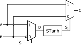
Fig. 3 shows the architecture of the SMax function proposed in [17], which is based on the stochastic comparator (input multiplexer and STanh function). The SMin function is obtained by swapping the input streams at the final multiplexer. The following proposition validates the correctness of the circuit shown in Fig. 3.
Proposition 1.
For uncorrelated input bit streams and , encoding the values and (unipolar coding format), the output of the circuit shown in Fig. 3 can be expressed as
| (13) |
where denotes the value encoded in the output stream . For the expression in (13) can be written as
| (14) |
which validates the functionality of the SMax function.
Proof.
The output of the first multiplexer is given by (cf. (4))
| (15) |
with . According to (10), the output of the STanh function can be expressed as
| (16) |
Finally, the output of the second multiplexer is given by (cf. (4))
| (17) | ||||
| (18) |
When substituting , and with their corresponding unipolar coding format values , and we obtain
| (19) |
Fig. 4 illustrates the analytical expression in (13), the bit-wise simulation results of the circuit shown in Fig. 3 and the exact max function. We observe a good match between the theoretical and simulation results. Moreover, we observe that already a moderate number of states provide a good approximation of the max function. inline]Fig.: Results for different states, Fig.: Verification of the analytical result, Fig./Table: Approx. Error
III-B Stochastic Max/Min Function in [23]
Fig. 5 shows the architecture of the SMax function proposed in [23]. Similar to Sec. III-A, the SMin function is obtained by swapping the input streams at the final multiplexer. The following proposition validates the correctness of the circuit shown in Fig. 5.
Proposition 2.
For uncorrelated input bit streams and , encoding the values and (unipolar coding format), the output of the circuit shown in Fig. 5 can be expressed as
| (20) |
where denotes the value encoded in the output stream . For the expression in (20) can be written as
| (21) |
which validates the functionality of the SMax function.
Proof.
The output of the XOR gate can be expressed as (cf. (6))
| (22) |
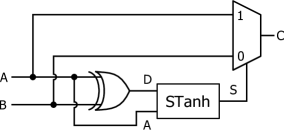
inline]Fig. of the new FSM In contrast to the STanh function presented in Sec. II-C1 the STanh function shown in Fig. 5 has two inputs and . The stochastic stream is used to enable the FSM state update and the updates the state according to its value. In particular, if then the state increases if and decreases if ; if the state is not updated independently of . Thus, the probability that the state increases or decreases is given by and , respectively. According to (8), the steady state probability is given by
| (23) |
with and . According to (10), the output of the STanh function can be expressed as
| (24) |
Finally, the output at the multiplexer is given by (cf. (4))
| (25) | ||||
| (26) |
For the unipolar encoding format (i.e. , and ) we have
| (27) |
Fig. 6 illustrates the analytical expression in (20), the bit-wise simulation results of the circuit shown in Fig. 5, and the exact max function. We observe a good match between the theoretical and simulation results. Similar to Fig. 4, we observe that already a moderate number of states provide a good approximation of the max function. However, in Fig. 6 one can already see a closer match of this approach compared to the SMax function of [17].
IV Novel Stochastic Max/Min Function: Architecture
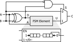
In this section, we propose a novel architecture for the SMax function as shown in Fig. 7. This circuit can be easily converted to realize the SMin function by inverting its inputs and as well as its output . Hence, we only consider the SMax function in the following description.
In contrast to the state-of-the-art SMax functions [23, 17], the FSM-based SC element used in the proposed architecture does not implement the STanh function. However, similar to the architecture in [23] it has two inputs and . Input enables the FSM state update and updates the state according to its value (cf. Sec. III-B). FSM-based elements can either be implemented using up/down counters or shift registers. When using a shift register, its length is equal to the last state of the FSM, i.e. . For the novel SMax function we use a shift register, since it has some distinct advantages compared to a counter-based implementation [10]. One advantage is that the values in a shift register are of equal significance, in contrast to a binary counter, where the bits are weighted by different powers of two. This allows to design more fault-tolerant SC computing circuits when using shift registers. Furthermore, as the following description demonstrates, shift registers are naturally suited to implement the described functionality.
Depending on the actual value of the input streams and the functionality of the SMax function (cf. Fig. 7) can be described as follows:
-
•
: Since the content of the shift register remains unchanged (state is not updated) and the output of the circuit is given by .
-
•
: Since and a zero is shifted from the right into the shift register (state is decremented) and the the output of the circuit is given by .
-
•
: Since and a one is shifted from the left into the shift register (state is incremented). In this case the rightmost value of the shift register is output by the circuit, i.e. .
According to the description above it is important to note that the ones in the stream also appear in the output stream .
In the following, we provide two approaches for analyzing the functionality of the proposed SMax function. First, we describe the functionality by considering the individual bits in the stochastic bit stream. Then, similar to Sec. III we proof the correctness of the circuit assuming very long stochastic bit streams. We denote these two methods as deterministic and probabilistic analysis, respectively.
IV-A Deterministic Analysis
For the deterministic analysis of the novel SMax function we distinguish the two cases: and .
IV-A1 SMax Circuit Behavior for
If , the stream has more (or equal) ones than bit stream . For a correct functionality it is desired that the number of ones in the input stream , and the number of ones in the output stream , are equal. As discussed above, all ones of stream are included in the output stream . However, if a subsequence of has more ones than the corresponding subsequence of , also ones of stream might be additionally injected into the output stream . This occurs if the excess of ones in this subsequence is larger than the shift register length . We refer to such an event as right overflow of the shift register. Thus, the number of ones in the output stream can be expressed as
| (28) |
where denotes the additional number of ones due to the right overflows. If the shift register is sufficiently long, no right overflows occur, i.e. .
IV-A2 SMax Circuit Behavior for
If , the bit stream has more ones than bit stream . For a correct functionality, it is desired that , the number of ones in the input stream , and , the number ones in the output stream , are identical. Similar as above, all ones of are included in the output stream . In addition, the excess of ones in stream is shifted into the shift register and once the shift register is filled, the ones are injected into the output stream when and occurs. However, at the end there might be ones left in the shift register, which are missing in the output stream555We assume the same length for all stochastic streams, which is a typically assumption in SC. . We denote the number of missing ones by .
Moreover, if a subsequence of has more ones than the corresponding subsequence of , also ones of stream might additionally be injected into the output stream . This happens if the excess of ones leads to an empty (all-zero) shift register, and, thus, an input pattern and (and assuming a later following and ) injects an additional one in the output stream . We refer to this effect as left overflow of the shift register and denote the number of additional ones due to left overflows by . This allows expressing the number of ones in the output stream as
| (29) |
where denotes the excess of ones in stream compared to stream . Expression (29) shows the two opposite error effects. One the one hand, the number of left overflows becomes smaller for long shift registers. On the other hand, the error due to the remaining ones in the shift register becomes smaller, for short shift registers. In Sec. V we determine the optimal shift register length for a given bit stream length.
IV-B Probabilistic Analysis
The following proposition validates the correctness of the circuit shown in Fig. 7.
Proposition 3.
For uncorrelated input bit streams and , encoding the values and (unipolar coding format), the output of the circuit shown in Fig. 7 can be expressed as
| (30) |
where denotes value encoded in the output stream . For the expression in (30) can be written as
| (31) |
which validates the functionality of the SMax function.
Proof.
The output of the XOR gate can be expressed as (cf. (6))
| (32) |
Similar to Sec. III-B, the FSM has two inputs and and, thus, the steady state probability can be written as (cf. (23))
| (33) |
According to Fig. 7, the FSM outputs can be expressed as
| (34) |
The output of the AND gate can be calculated as (cf. (4))
| (35) |
Finally, the output of the multiplexer is given by
| (36) |
For the unipolar encoding format (i.e. , and ) we have
| (37) |
Fig. 8 illustrates the analytical expression in (30), the bit-wise simulation results of the circuit shown in Fig. 7 and the exact max function. We observe a good match between the theoretical and simulation results. Moreover, we observe that already a low number of states provide a good approximation of the max function. In contrast to the state-of-the-art SMax functions [17, 23] the proposed function does not approach the exact max function at , but provides a better approximation for .
Next, we compare the approximation error of the state-of-the-art SMax functions and the novel SMax function. For this we calculate the expected value of the absolute error, assuming a uniform distribution of and over the interval , respectively. We define the absolute error by , with the exact max function and the FSM-based approximations given in (13), (20) and (30), respectively. Then, the expected absolute error can be calculated as
| (38) |
The absolute value of the error in (38) allows to consider both, erroneously added ones (i.e. ) as well as erroneously removed ones (i.e. ) in the bit stream representing . When considering a stochastic bit stream of , then the absolute difference can be interpreted as a bit error probability of compared to such a bit stream of . This is crucial in order to enable a comparison with the analysis results presented in Sec. V. We observe from Fig. 9 that the novel SMax function has a significantly lower approximation error than the state-of-the-art SMax functions. This is because the denominator of (30) (power of ) converges faster to zero or infinity as the number of states increases compared to the denominators in (13) or (20) (power of ). Moreover, we observe that the SMax function proposed in [17] has the highest approximation error among the three approaches.
V Novel Stochastic Max/Min Function: Error Analysis
We observed from the deterministic analysis in Sec. IV-A that long shift registers reduce the errors due to right and left overflows. However, a large shift register length increases the error caused by the remaining bits in the shift register. It is important to note that especially the last observation cannot be inferred from the probabilistic analysis presented in the previous chapter. The probabilistic analysis becomes exact if and only if the bit stream length goes to infinity. In such a case, a finite number of remaining bits in the shift register does not matter. However, when using a finite bit stream length, these remaining bits matter. In the following analysis, we assume a finite bit stream length that is significantly larger than the shift register length (a typical scenario in SC). This allows using the probabilistic FSM description in Sec. IV-B for modelling the behavior of the shift register for finite bit stream lengths. Moreover, having sufficiently long bit streams justifies using the probabilities of ones instead of the rate of ones in the stream (cf. Sec. II-A) for the following error analysis.
In the following, we derive the expected error probability, based on the deterministic analysis in Sec. IV-A. With this expression we determine the optimal shift register length , with respect to the bit stream length . Similar to Sec. IV-A we distinguish two cases: and .
V-A Error Probability for
In this case, an error occurs due to right overflows. In particular, the shift register is filled with ones, i.e. the FSM is in the last state , and the input and is applied. The probability for this error event can be described as
| (39) |
where describes the probability of the FSM to be in the last state (cf. (34)).
V-B Error Probability for
In this case, errors can originate from two sources: Left overflow and remaining ones in the shift register. At the left overflow, the shift register is empty (all-zeros), i.e. the FSM is in state , and the input pattern and occurs. The probability for this error event can be expressed as
| (40) |
where denotes the probability of the zero state of the FSM, i.e. an all-zero shift register (cf. (33)). The corresponding expected number of erroneously added ones in the output stream can be calculated by
| (41) |
For the error caused by the remaining ones in the shift register we compute the expected value of the shift register state, i.e. the expected number of ones in the shift register, as
| (42) |
where denotes the probability of the FSM to be in the th state. Note that the expected number of ones in the shift register corresponds to the number of ones that are missing on average in the output stream. Combining (41) and (42) and considering that left overflows add ones to the output stream, while the remaining bits in the shift register are the missing ones in the output stream, the expected number of erroneous ones is given by
| (43) |
Finally, the error probability can be expressed as
| (44) |
Interestingly, the second term in (44) depends on the stream length , which goes to zero for . This is because a finite number of missing bits has a higher impact on the error for shorter streams than for longer streams.
V-C Expected Error Probability
Assuming a uniform distribution for and over and using (39) and (44), the expected error probability can be derived as follows
| (45) |
The two integrals in (45), cover exactly half of the two dimensional space . Thus, they form the expected value over the whole space.
Unfortunately, to the best of our knowledge, for this integral no closed-form solution exists. Thus, we calculated it through numerical integration. Fig. 10 shows the error probabilities obtained through numerical integration and the simulation results. For each simulated point, the empirical error probability was averaged over test cases. We observe a good match between the theoretical and the simulation results. However, the analytical results are obtained much faster than the simulation results. Moreover, it can be seen that for a certain stream length there exists an optimal shift register length . For example, for the error probability decreases until length and then increases due to the remaining bits in the shift register. Thus, for the optimal shift register length is given by . In Fig. 10, we marked the optimal shift register lengths with triangles and added extra ticks at the x-axis. The lower bound curve in Fig. 10 corresponds to the performance limit if the bit stream length goes to infinity. It can either be obtained by numerically integrating (38) or (45), the latter with . For the latter approach, the second term on the right hand side of (44) goes to zeros, resulting in . This is because when the stream length goes to infinity, a finite number of remaining bits in the shift register does not matter.
VI Conclusions
In this work, we investigated the stochastic SMax/SMin function, which is an important building block in many applications (e.g., max pooling in neural networks). Prior works have proposed circuits for the SMax/SMin function and provided empirical validation. In this paper, we analytically proved the correctness of these architectures. Moreover, we proposed a novel shift-register based SMax/SMin function, which outperforms the state-of-the-art architectures in terms of accuracy, while having comparable hardware cost. We provided a new error analysis of the proposed circuit, considering the value of the individual bits in the stochastic stream. This analysis revealed that for practical bit stream lengths a finite optimal shift register length exists. Moreover, we showed that increasing the shift register length beyond the optimal value deteriorates the accuracy. This is due to the error caused by the remaining bits in the shift register. Hence, finding strategies to empty the shift register might be an interesting future extension of this work.
References
- [1] B. R. Gaines, Stochastic Computing Systems. Boston, MA: Springer US, 1969, pp. 37–172.
- [2] A. Alaghi and J. P. Hayes, “Survey of stochastic computing,” ACM Trans. Embed. Comput. Syst., vol. 12, no. 2s, pp. 92:1–92:19, May 2013.
- [3] A. Alaghi, W. Qian, and J. P. Hayes, “The promise and challenge of stochastic computing,” IEEE Trans. Comput.-Aided Design Integr. Circuits Syst., pp. 1–1, 2017.
- [4] P. Li, D. J. Lilja, W. Qian, M. D. Riedel, and K. Bazargan, “Logical computation on stochastic bit streams with linear finite-state machines,” IEEE Trans. Comput., vol. 63, no. 6, pp. 1474–1486, June 2014.
- [5] M. H. Najafi and M. E. Salehi, “A fast fault-tolerant architecture for sauvola local image thresholding algorithm using stochastic computing,” IEEE Trans. VLSI Syst., vol. 24, no. 2, pp. 808–812, Feb. 2016.
- [6] W. Qian, M. D. Riedel, and I. Rosenberg, “Uniform approximation and bernstein polynomials with coefficients in the unit interval,” European Journal of Combinatorics, vol. 32, no. 3, pp. 448 – 463, 2011.
- [7] W. Qian, X. Li, M. D. Riedel, K. Bazargan, and D. J. Lilja, “An architecture for fault-tolerant computation with stochastic logic,” IEEE Trans. Comput., vol. 60, no. 1, pp. 93–105, Jan 2011.
- [8] W. Qian and M. D. Riedel, “The synthesis of robust polynomial arithmetic with stochastic logic,” in ACM/IEEE Design Automation Conference, June 2008, pp. 648–653.
- [9] B. D. Brown and H. C. Card, “Stochastic neural computation. I. Computational elements,” IEEE Trans. Comput., vol. 50, no. 9, pp. 891–905, Sep 2001.
- [10] P. Ting and J. P. Hayes, “On the role of sequential circuits in stochastic computing,” in Proc. of the on Great Lakes Symposium on VLSI, ser. GLSVLSI ’17, 2017, pp. 475–478.
- [11] M. H. Najafi, P. Li, D. J. Lilja, W. Qian, K. Bazargan, and M. Riedel, “A reconfigurable architecture with sequential logic-based stochastic computing,” J. Emerg. Technol. Comput. Syst., vol. 13, no. 4, pp. 57:1–57:28, Jun. 2017.
- [12] V. C. Gaudet and A. C. Rapley, “Iterative decoding using stochastic computation,” Electronics Letters, vol. 39, no. 3, pp. 299–301, Feb 2003.
- [13] Q. T. Dong, M. Arzel, C. Jego, and W. J. Gross, “Stochastic decoding of turbo codes,” IEEE Trans. Signal Process., vol. 58, no. 12, pp. 6421–6425, Dec 2010.
- [14] X. R. Lee, C. L. Chen, H. C. Chang, and C. Y. Lee, “A 7.92 gb/s 437.2 mw stochastic LDPC decoder chip for IEEE 802.15.3c applications,” IEEE Trans. Circuits Syst. I, vol. 62, no. 2, pp. 507–516, Feb 2015.
- [15] S. L. T. Marin, J. M. Q. Reboul, and L. G. Franquelo, “Digital stochastic realization of complex analog controllers,” IEEE Trans. Ind. Electron., vol. 49, no. 5, pp. 1101–1109, Oct 2002.
- [16] D. Zhang and H. Li, “A stochastic-based FPGA controller for an induction motor drive with integrated neural network algorithms,” IEEE Trans. Ind. Electron., vol. 55, no. 2, pp. 551–561, Feb 2008.
- [17] P. Li and D. J. Lilja, “Using stochastic computing to implement digital image processing algorithms,” in 2011 IEEE 29th International Conference on Computer Design (ICCD), Oct 2011, pp. 154–161.
- [18] A. Alaghi, C. Li, and J. P. Hayes, “Stochastic circuits for real-time image-processing applications,” in Proc. Design Automation Conf., May 2013, pp. 1–6.
- [19] P. Li, D. J. Lilja, W. Qian, K. Bazargan, and M. D. Riedel, “Computation on stochastic bit streams digital image processing case studies,” IEEE Trans. VLSI Syst., vol. 22, no. 3, pp. 449–462, March 2014.
- [20] H. Ichihara, T. Sugino, S. Ishii, T. Iwagaki, and T. Inoue, “Compact and accurate digital filters based on stochastic computing,” IEEE Trans. Emerg. Topics Comput., pp. 1–1, 2017.
- [21] Y. N. Chang and K. K. Parhi, “Architectures for digital filters using stochastic computing,” in Proc. Int. Conf. Acoustics, Speech and Signal Processing, May 2013, pp. 2697–2701.
- [22] A. Ren, Z. Li, C. Ding, Q. Qiu, Y. Wang, J. Li, X. Qian, and B. Yuan, “SC-DCNN: highly-scalable deep convolutional neural network using stochastic computing,” in Proc. Conf. Architectural Support for Programming Languages and Operating Systems, ser. ASPLOS ’17. New York, NY, USA: ACM, 2017, pp. 405–418.
- [23] J. Yu, K. Kim, J. Lee, and K. Choi, “Accurate and efficient stochastic computing hardware for convolutional neural networks,” in 2017 IEEE International Conference on Computer Design (ICCD), Nov 2017, pp. 105–112.
- [24] B. D. Brown and H. C. Card, “Stochastic neural computation. II. Soft competitive learning,” IEEE Trans. Comput., vol. 50, no. 9, pp. 906–920, Sep 2001.