Low-power phonon lasing through position-modulated Kerr-type nonlinearity

Abstract

We demonstrate low-power amplification process in cavity optomechanics (COM). This operation is based on the nonlinear position-modulated self-Kerr interaction. Owing to this nonlinear term, the effective coupling highly scales with the photon number, resulting in a giant enhancement of the cooperativity. Even for small nonlinearity, the system reaches the amplification threshold for weak driving strength, leading to low-power phonon lasing. This amplifier can be phase-preserving and provides a practical advantage related to the power consumption issues. This work opens up new avenues to realize low-power and efficient amplifiers in optomechanics and related fields.

I Introduction

Cavity optomechanics (COM), which is devoted to explore interaction between electromagnetic radiation and mechanical object, provides a platform to perform phonon lasing action [1] , [2] based on backaction amplification [3] . At the threshold of parametric instability, backaction-induced mechanical gain overcomes mechanical loss, resulting to an amplification process that leads to coherent phonon oscillations [1] . Similar to stimulated emission of photon lasing in cavity with a gain medium, backaction amplification induces stimulated phonon lasing from the parametric instability’s threshold [4] . Both phonon lasing and amplification are actively studied in optomechanics, and other fields, for technological purposes.

Single-phonon Fock state detection has been recently performed in [5] , [6] , and that paves a way to variety of quantum state engineering tasks including, quantum information processing [7] and quantum entanglement of remote mechanical elements [8] . The developpment of single phonon source reveals also a process towards technologies for precision sensing [9] . Moreover, intensive researches are carried out in order to improve these achievements, for instance to lower the power need for phonon lasing. Such performance has been recently realized using $\mathcal{PT-}$symmetry optomechanics [10] , and the polarization of light in coupled optomechanical devices [11] .

To use quantum signals, those involving only a few quanta, they need to be amplified and must display some degree of purity to carry certain amount of information. This issue can be handled by characterizing the amplification process as the system gets closer to the phonon lasing threshold. These characteristics include phase-preserving amplification [12] , [13] , [14] , the power gain and the number of added noise, and the gain-bandwidth product [15] , [16] , [17] , [18] . The purpose of a phase-preserving amplifier is to make a weak signal large, regardless of its phase, so that it can be perceived by devices unable to resolve the original signal, while sacrificing as little as possible in signal-to-noise ratio [14] . Engineering amplifier having large power gain with quantum-limited added noise [17] , [18] , and without limitation on the gain-bandwidth product [17] are useful for applications such as sensing [3] , [9] and quantum information processing [7] . However, amplifying (or reaching phonon lasing threshold) with low-power consumption would provide practical advantage for amplifiers. Such low-power light amplifier has been recently realized, and has shown high gain at low-power operation and low quantum limit noise performance [19] .

Recently, nonlinear position-modulated self-Kerr interaction has been engineered in COM, and it was found that it leads to an effective coupling that scales with the square of the photon number [20] . Such nonlinearity can be derived in the situation where Kerr nonlinear coefficient is modulated by the mechanical position. Such an interaction is possible in superconducting systems, cavity polaritonic systems, and atom-optical systems. It has been shown that this nonlinearity leads to a strong coupling, even for low driving strength. Moreover, these authors have demonstrated motional cooling, mode splitting and multistability for low-power red driving. Owing to these interesting nonlinear phenomena, our aim here is to perform low-power phonon laser at the blue sideband, resulting from low-power amplification induced by this nonlinearity. To understand this low-power operation, we have derived the cooperativity that highly scales with the photon number. This pushes the system fastly near to the amplification’s threshold. We have characterized the amplifier, that shows high gain and phase-preserving close to the phonon lasing threshold. This work opens up promising ways to develop low-power amplifiers based on the position-modulated self-Kerr interaction in COMs and superconducting (electromechanical) microwave setups [21] , [22] .

II Results

II.1 Hamiltonian and dynamical equations

Position-modulated self-Kerr nonlinearity can be engineered in COMs [23] , [24] , [25] or in the electromechanical microwave setups exhibiting a giant Kerr nonlinearity [21] , [22] . The idea of this engineering is based on the fact that, the Kerr nonlinear coefficient is modulated by the position of the mechanical resonator connected to the system. Such nonlinear interaction, has been recently investigated in [20] . This has led to an effective coupling that scales with the square of the photon number. In the red sideband, this effective coupling leads to low powers required for motional cooling, the emergence of multistability, and other interesting nonlinear features. Owing to these exciting nonlinear effects, here we move to the blue sideband and investigate on phonon lasing and amplification phenomena. The Hamiltonian describing the generic system, with $\hbar=1$, is given by,

$$H=-\Delta_{0}a^{{\dagger}}a+\omega_{m}b^{{\dagger}}b-g_{l}a^{{\dagger}}a(b^{{\dagger}}+b)-g_{nl}a^{{\dagger}}a^{{\dagger}}aa(b^{{\dagger}}+b)+E(a+a^{{\dagger}}).$$ (1)

In this Hamiltonian, $a$ ($b$) is the annihilation bosonique operator for the intracavity field (mechanical resonator), $H_{l,int}=-g_{l}a^{{\dagger}}a(b^{{\dagger}}+b)$ and $H_{nl,int}=-g_{nl}a^{{\dagger}}a^{{\dagger}}aa(b^{{\dagger}}+b)$ describe the linear and nonlinear interactions. The first two terms represent the cavity and mechanical free energy respectively, while the last term stand for the driving energy. The parameters $\omega_{m}$ and $\Delta_{0}=\omega_{p}-\omega_{cav}$ are the mechanical frequency of the resonator and the detuning between the optical drive ($\omega_{p}$) and the cavity eigenfrequency ($\omega_{cav}$). The linear and nonlinear optomechanical couplings are denoted by $g_{l}$ and $g_{nl}$, respectively. The mechanical displacement is defined as $x=x_{ZPF}(b+b^{{\dagger}})$, where $x_{ZPF}=\sqrt{\tfrac{\hbar}{2m\omega_{m}}}$ is the zero-point fluctuation amplitude of the mechanical resonator, with $m$ its effective mass. In the driving rotating frame, the Nonlinear Langevin Equations (NLEs), including cavity ($\kappa$) and mechanical ($\gamma_{m}$) dissipations, can be derived as follows,

$$\left\{\begin{array}[]{c}\dot{a}=\left[i\left(\Delta_{0}+g_{l}(b^{{\dagger}}+b)+2g_{nl}(b^{{\dagger}}+b)a^{{\dagger}}a\right)-\frac{\kappa}{2}\right]a-iE,\\ \dot{b}=-\left(i\omega_{m}+\frac{\gamma_{m}}{2}\right)b+ig_{l}a^{{\dagger}}a+ig_{nl}a^{{\dagger}}a^{{\dagger}}aa.\end{array}\right.$$ (2)

Throughout the work, we assume the hierarchy of parameters $\gamma_{m},g_{l}\ll\kappa\ll\omega_{m}$, similar to the experiments carried out in the resolved sideband regime [5] ,[6] . Our numerical and analytical investigations will be done at the sideband $\Delta_{0}=\omega_{m}$. To get insight of the phonon lasing phenomenon, we linearize Eq. (2) in the limit of large driving field. In this case, both intracavity field ($a$) and mechanical degrees of freedom ($b$) can be splitted into their average fields ($\alpha(t)$, $\beta(t)$) with some amount of fluctuations ($\delta\alpha(t)$, $\delta\beta(t)$) as follows,

$$\left\{\begin{array}[]{c}\delta\alpha(t)=a(t)-\alpha(t),\\ \delta\beta(t)=b(t)-\beta(t).\end{array}\right.$$ (3)

Using Eq. (3) in Eq. (2), leads to the steady-state dynamics,

$$\left\{\begin{array}[]{c}\dot{\alpha}=\left(i\Delta-\frac{\kappa}{2}\right)\alpha+\sqrt{\kappa}\alpha^{in},\\ \dot{\beta}=-\left(i\omega_{m}+\frac{\gamma_{m}}{2}\right)\beta+ig_{l}\left|\alpha\right|^{2}+ig_{nl}\left|\alpha\right|^{4},\end{array}\right.$$ (4)

with the corresponding lowest order fluctuations dynamics, including noises,

$$\left\{\begin{array}[]{c}\delta\dot{\alpha}=\left(i\Delta-\frac{\kappa}{2}\right)\delta\alpha+i\chi\left(\delta\beta^{\ast}+\delta\beta\right)+i\eta\left(\delta\alpha^{\ast}+\delta\alpha\right)+\sqrt{\kappa}\delta\alpha^{in},\\ \delta\dot{\beta}=-\left(i\omega_{m}+\frac{\gamma_{m}}{2}\right)\delta\beta+i\chi\left(\delta\alpha^{\ast}+\delta\alpha\right)+\sqrt{\gamma_{m}}\delta\beta^{in}.\end{array}\right.$$ (5)

In Eq. (4) and Eq. (5), we have set for convenience $-iE=\sqrt{\kappa}\alpha^{in}$ [18] where the driving strength $\alpha^{in}$ is related to the input power $P_{in}$ as $\alpha^{in}=\sqrt{\frac{P_{in}}{\hbar\omega_{p}}}$. We have defined the effective coupling as $\chi=\chi_{0}\alpha$ with $\chi_{0}=(g_{l}+2g_{nl}|\alpha|^{2})$, $\eta=4g_{nl}|\alpha|^{2}\rm{Re}(\beta)$ and $\Delta=\Delta_{0}+2\chi_{0}\rm{Re}(\beta)$. The noise operators are characterized by the noncommuting properties, i.e., $\langle\delta\alpha^{in}(t)\rangle=0$, $\langle\delta\alpha^{in{\dagger}}(t^{{}^{\prime}})\delta\alpha^{in}(t)\rangle=n_{\alpha}\delta(t^{{}^{\prime}}-t)$, and $\langle\delta\alpha^{in}(t^{{}^{\prime}})\delta\alpha^{in{\dagger}}(t)\rangle=(n_{\alpha}+1)\delta(t^{{}^{\prime}}-t)$ for the input field and $\langle\delta\beta^{in}(t)\rangle=0$, $\langle\delta\beta^{in{\dagger}}(t^{{}^{\prime}})\delta\beta^{in}(t)\rangle=n_{th}\delta(t^{{}^{\prime}}-t)$, and $\langle\delta\beta^{in}(t^{{}^{\prime}})\delta\beta^{in{\dagger}}(t)\rangle=(n_{th}+1)\delta(t^{{}^{\prime}}-t)$ for the thermal bath. The quantities $n_{\alpha}$ and $n_{th}$ are the equilibrium occupation numbers for the input field and mechanical oscillator, respectively.

II.2 Stability

The steady-state solutions $\alpha_{s}$ and $\beta_{s}$ are derived from Eq. (4), providing $\dot{\alpha}=0$ and $\dot{\beta}=0$. These solutions are given by,

$$\left\{\begin{array}[]{c}\alpha_{s}=\frac{\sqrt{\kappa}\alpha^{in}}{\left(\frac{\kappa}{2}-i\left[\Delta_{0}+2\chi_{0}\rm{Re}(\beta_{s})\right]\right)},\\ \beta_{s}=\left(g_{l}+g_{nl}\left|\alpha_{s}\right|^{2}\right)\frac{\left|\alpha_{s}\right|^{2}}{\omega_{m}-i\frac{\gamma_{m}}{2}}.\end{array}\right.$$ (6)

By setting the intracavity intensity as $I=|\alpha_{s}|^{2}$, one shows from Eq. (6) that it is solution of the following seventh-order polynomial equation,

$$I^{7}+a_{6}I^{6}+a_{5}I^{5}+a_{4}I^{4}+a_{3}I^{3}+a_{2}I^{2}+a_{1}I+a_{0}=0,$$ (7)

with $a_{6}=\frac{3g_{l}}{g_{nl}}$; $a_{5}=\frac{13g_{l}^{2}}{4g_{nl}^{2}}$; $a_{4}=\frac{3g_{l}^{3}+\Delta\omega_{m}g_{nl}}{2g_{nl}^{3}}$; $a_{3}=\frac{g_{l}(g_{l}^{3}+3\Delta\omega_{m}g_{nl})}{4g_{nl}^{4}}$; $a_{2}=\frac{\Delta\omega_{m}g_{l}^{2}}{4g_{nl}^{4}}$; $a_{1}=\frac{(\frac{\kappa^{2}}{4}+\Delta^{2})\omega_{m}^{2}}{(2g_{nl})^{4}}$; $a_{0}=-\frac{\kappa(\alpha^{in}\omega_{m})^{2}}{(2g_{nl})^{4}}$. These steady state solutions are physically meaningless, unless they are stable. The stability can be given explicitly through Routh-Hurwitz criterion [25] . However, we analyze it here through linear stability theory, and confirm it with parametric instability threshold, since we are in the blue sideband regime. To this end, we start by writing Eq. (5) in the follwing compact form,

$$\delta\dot{X}=M\delta X+\epsilon,$$ (8)

with $\delta X=(\delta\beta,\delta\beta^{\ast},\delta\alpha,\delta\alpha^{\ast})^{T}$ and $\epsilon=(\sqrt{\gamma_{m}}\delta\beta^{in},\sqrt{\gamma_{m}}\delta\beta^{in\ast},\sqrt{\kappa}\delta\alpha^{in},\sqrt{\kappa}\delta\alpha^{in\ast})^{T}$. The matrix $M$ is given by,

$$M=\begin{bmatrix}-(i\omega_{m}+\frac{\gamma_{m}}{2})&0&i\chi&i\chi\\ 0&(i\omega_{m}-\frac{\gamma_{m}}{2})&-i\chi&-i\chi\\ i\chi&i\chi&(i\tilde{\Delta}-\frac{\kappa}{2})&i\eta\\ -i\chi&-i\chi&-i\eta&-(i\tilde{\Delta}+\frac{\kappa}{2})\end{bmatrix},$$ (9)

with $\tilde{\Delta}=\Delta+\eta$, and where $\alpha_{s}$ is assumed to be real ($\alpha_{s}\in\mathbb{R}$).

The system is stable if all the real part of eigenvalues ($\lambda_{i=1..4}$) of the matrix $M$ are negative ($\rm{Re}(\lambda_{i=1..4})<0$). This stability depends on steady-state solutions $\alpha_{s}$ and $\beta_{s}$, and is shown in Fig. 1a.

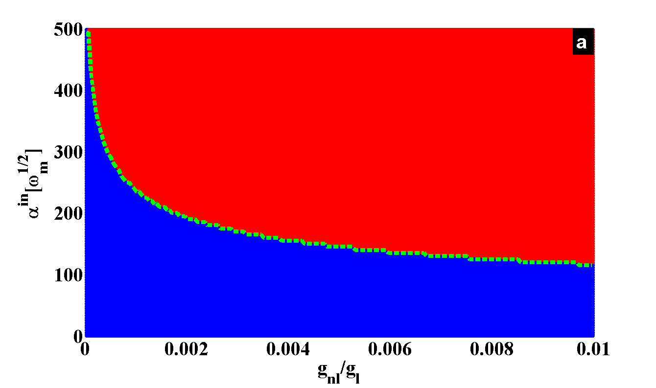
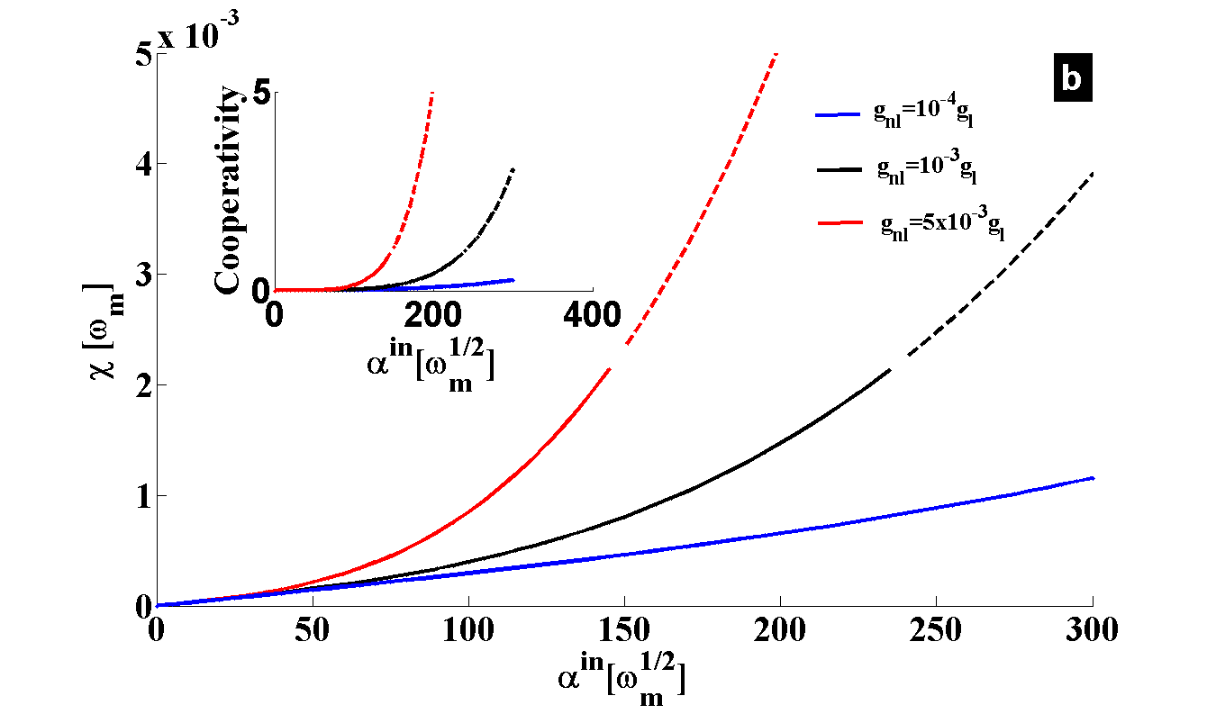
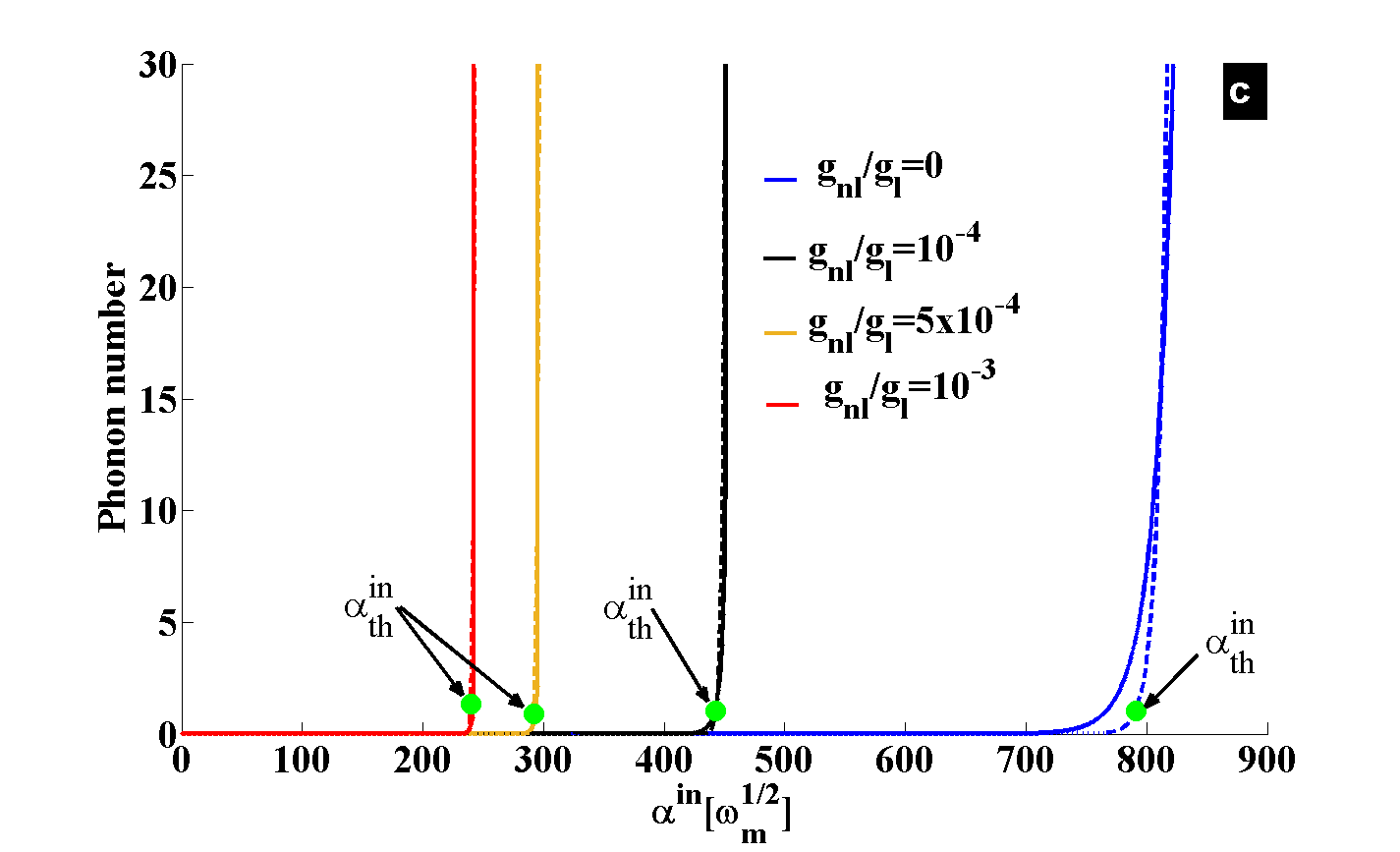
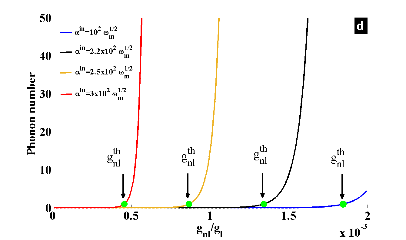
Figure 1: (a) Stability diagram. Blue (red) color is stable (unstable). The green dashed curve shows the border between stable and unstable regions, and corresponds to the lasing threshold $\mathcal{C}=1$, with the cooperativity $\mathcal{C}=4\chi^{2}/(\gamma_{m}\kappa)$. (b) Effective coupling $\chi$ versus $\alpha^{in}$ for different values of $g_{nl}$. Full (dashed) curves are stable (unstable). The inset shows the cooperativity $\mathcal{C}$ versus $\alpha^{in}$, for the corresponding values of $g_{nl}$. (c) Phonon number versus $\alpha^{in}$. Full curves are from numerical simulation of classical version of Eq. (2), while the dashed ones are the analytical approximation from $N\sim\rm{exp(-\gamma_{eff}t)}$. (d) Analytical (approximated) phonon number versus $g_{nl}$. In (c) and (d), the different lasing thresholds are indicated by the green dots. The used parameters are [20] ,[22] , $\gamma_{m}=10^{-3}\omega_{m}$, $\kappa=2\times 10^{-2}\omega_{m}$, $g_{l}=2\times 10^{-5}\omega_{m}$, and $\Delta_{0}=\omega_{m}$.

The blue color in Fig. 1a depicts stable parameters space, while the red area shows the unstable zone. As the self-Kerr term ($g_{nl}$) is increasing, the system becomes unstable and the stability is limited for relatively weak driving strength $\alpha^{in}$. The green dashed line in Fig. 1a holds for the condition $\mathcal{C}=1$, where $\mathcal{C}=4\chi^{2}/(\gamma_{m}\kappa)=\gamma_{opt}/\gamma_{m}$ is the cooperativity. This cooperativity, with $\gamma_{opt}$ being the optical damping, depicts the border between stable (linear) and unstable (nonlinear) regimes. Moreover, $\mathcal{C}=1$ defines the threshold of the phonon lasing in the optomechanical blue sideband. It results that the self-Kerr nonlinearity induces low power phonon lasing action, that can be understood by the enhancement of the effective coupling ($\chi$) shown in Fig. 1b. This coupling enhancement is a direct consequence of the fact that $\chi$ highly scales with the photon number in the presence of $g_{nl}$, resulting in a large cooperativity (see inset of Fig. 1b). Hence, as $g_{nl}$ increases, the lasing threshold is shifted towards weak driving strength $\alpha^{in}$, revealing low-power phonon lasing in our proposal.

II.3 Low power phonon lasing

To evaluate the stimulated emission phonon number, we have simulated the classical equivalent of the nonlinear equation given in Eq. (2). This is valid for large enough photon number in the system ($|\alpha|^{2}\gg 1$), so that both fluctuations from intracavity field and mechanical resonator can be neglected. By Fast Fourier Transforming (FFT) the results, and collecting the mechanical peak at the resonance, we have obtained the phonon number versus the driving $\alpha^{in}$, depicted in Fig. 1c. Full and dashed lines in Fig. 1c show the numerical and analytical results, respectively. This yields good agreement between numerical calculation and analytics, that is detailed in section III. Lasing threshold depicted by green dots are given by the condition $\gamma_{m}=\gamma_{opt}$ (or $\mathcal{C}=1$). As $g_{nl}$ is increasing, Fig. 1c reveals a low driving strength $\alpha^{in}$ required for phonon lasing threshold. In Fig. 1d, we have represented the phonon number versus $g_{nl}$ for different $\alpha^{in}$. It results that $g_{nl}$ enhances stimulated emission of phonons. Indeed, for $g_{nl}\sim 0$, there is no lasing up to $\alpha^{in}=3\times 10^{2}\sqrt{\omega_{m}}$ in Fig. 1d. Therefore, by adding a small amount of nonlinearity to the system, the lasing threshold rises up and is shifted towards small $g_{nl}$ as $\alpha^{in}$ increases. Briefly speaking, the higher is the driving strength, smaller is the amount of nonlinearity ($g_{nl}$) to reach the lasing threshold, and vice-versa. This can be understood from the dynamics of $b(t)$ in Eq. (2), showing that $g_{nl}$ supplies energy ($\propto g_{nl}|\alpha|^{4}$) to drive the mechanical resonator. This reveals why self-Kerr nonlinearity studied here, is quite interesting and different from Kerr nonlinearity [23] , [24] , [25] , [21] , quadratic nonlinearity [26] and Duffing nonlinearities [27] also studied in optomechanics.

II.4 Low power amplification

As self-Kerr nonlinearity enhances low-power phonon lasing (Fig. 1c), this also reveals low-power amplification process in the system. The feature of the nondegenerate parametric amplifier here is to convert a pump mode photon into, one photon signal mode and one idler phonon mode. This leads to the fact that weak incident signals are amplified, with a minimum possible added noise. Such amplification process can be seen from the linearization of the interaction Hamiltonian of our system. Indeed, the interaction of our system is captured by the Hamiltonian,

$$H_{int}=H_{l,int}+H_{nl,int}=-g_{l}a^{{\dagger}}a(b^{{\dagger}}+b)-g_{nl}a^{{\dagger}}a^{{\dagger}}aa(b^{{\dagger}}+b),$$ (10)

which leads to its linearized form,

$$H_{int}^{lin}=-\chi(\delta\alpha^{{\dagger}}\delta\beta^{{\dagger}}+\delta\alpha\delta\beta)-\chi(\delta\alpha^{{\dagger}}\delta\beta+\delta\alpha\delta\beta^{{\dagger}}),$$ (11)

after have used Eq. (3). Furthermore, Eq. (11) has been obtained by omitting static terms since they are taking into account in the frequency shift $\tilde{\Delta}$, and the higher order fluctuations terms have been neglected as being smaller than $\alpha_{s}$. The second term on the right-hand side of Eq. (11) stands for the counter rotating terms $H_{CR}=-\chi(\delta\alpha^{{\dagger}}\delta\beta+\delta\alpha\delta\beta^{{\dagger}})$ and can be neglected in the rotating wave approximation (RWA) [1] . However, the first term ($H_{R}=-\chi(\delta\alpha^{{\dagger}}\delta\beta^{{\dagger}}+\delta\alpha\delta\beta))$ describes a nondegenerate parametric amplifier, where a pump mode (photon) is converted into two quanta, one in the signal mode (photon), and the other in the idler (phonon). To characterize this amplifier, we neglect non resonant terms in Eq. (5) and rewrite it in the RWA as,

$$\left\{\begin{array}[]{c}\delta\dot{\alpha}=(i\Delta-\frac{\kappa}{2})\delta\alpha+i\chi\delta\beta^{{\dagger}}+\sqrt{\kappa}\delta\alpha^{in},\\ \dot{\delta\beta}^{{\dagger}}=(i\omega_{m}-\frac{\gamma_{m}}{2})\delta\beta^{{\dagger}}-i\chi\delta\alpha+\sqrt{\gamma_{m}}\delta\beta^{in}.\end{array}\right.$$ (12)

By solving Eq. (12) in the Fourier space, together with the input-output relation, $\delta\alpha^{out}=\delta\alpha^{in}-\sqrt{\kappa}\delta\alpha$ [15] , [18] , we can evaluate the output field $\delta\alpha^{out}$. This output field is a key element to characterize the gain and added noise of the amplifier. More details on calculations leading to the gain and added noise are reported in section III, while specific results are shown in what follows. The input-output relation leads to the output field,

$$\delta\alpha^{out}=(1-\sqrt{\kappa}\chi_{eff}^{c})\delta\alpha^{in}-i\sqrt{\kappa}\eta_{c}\delta\beta^{in{\dagger}},$$ (13)

where

$$\eta_{c}=\frac{\chi_{m}\chi_{c}\chi\sqrt{\gamma_{m}}}{1-\chi_{m}\chi_{c}\chi^{2}};\chi_{eff}^{c}=\frac{\chi_{c}\sqrt{\kappa}}{1-\chi_{m}\chi_{c}\chi^{2}},$$ (14)

with the susceptibilities $\chi_{c}=\left[\frac{\kappa}{2}-i(\omega+\tilde{\Delta})\right]^{-1}$, and $\chi_{m}=\left[\frac{\gamma_{m}}{2}-i(\omega+\omega_{m})\right]^{-1}$. In Eq. (13), the coefficient in front of the incident signal $\delta\alpha^{in}$ characterizes the amplification gain, while the one in front of the thermal noise informs on the added noise. These characteristics are deduced from the output noise power spectral density (PSD) defined as [17] , [18] ,

$$S_{out}=\frac{1}{2}\left(\langle\delta\alpha^{out{\dagger}}\delta\alpha^{out}+\delta\alpha^{out}\delta\alpha^{out{\dagger}}\rangle\right).$$ (15)

The output PSD ($S_{out}$) is shown in Fig. 2a, and reveals an amplification process at the resonance $\omega=-\Delta$, induced by the nonlinear term $g_{nl}$. For $\alpha^{in}=2\times 10^{2}\sqrt{\omega_{m}}$ and $g_{nl}\leq 1\times 10^{-3}$, there is no amplification as shown in Fig. 1c. However, for $g_{nl}\approx 1.85\times 10^{-3}$, Fig. 2a clearly shows amplification, meaning that $g_{nl}$ brings the system near the lasing threshold even for a weak driving strength. In order to appreciate this amplification, the output PSD has been plotted at the resonance $\omega=-\Delta$ (for $\alpha^{in}=2\times 10^{2}\sqrt{\omega_{m}}$) versus $g_{nl}$, and shown in Fig. 2b. The red and black curves correspond to ($n_{\alpha}=1$, $n_{th}=1$) and ($n_{\alpha}=1$, $n_{th}=0$), respectively. It results that thermal noise has an impact on the amplification, revealing the effect of the added noise on the amplifier. This can be pointed out by evaluating both the power gain $\mathcal{G}(\omega)$ and the added noise $\mathcal{N}(\omega)$. The amplification of the signal $\delta\alpha^{in}$ is measured through the gain $|1-\sqrt{\kappa}\chi_{eff}^{c}|^{2}$, which can be simplified (see section III) at the resonance ($\omega=-\Delta$) as,

$$\mathcal{G}=\left|\frac{\mathcal{C}+1}{1-\mathcal{C}}\right|^{2}.$$ (16)

The noise performance of the amplifier is figured out through the input-referred added noise, defined as $\mathcal{N}(\omega)=\left(S_{out}-S_{in}\right)/\mathcal{G}^{2}$, where $S_{in}=\frac{1}{2}$ is the vacuum input noise driving the cavity. As shown in section III, this expression reduces at the resonance to,

$$\mathcal{N}=\frac{4\mathcal{C}\left(n_{eff}+\frac{1}{2}\right)}{\left|\mathcal{C}+1\right|^{2}},$$ (17)

where $n_{eff}=n_{th}+n_{\alpha}$ is the effective phonon number of the mechanical resonator. Eq. (16) shows that the gain exponentially grows as the system approaches the lasing threshold at a cooperativity $\mathcal{C}\rightarrow 1$, revealing the amplification process. As $\mathcal{C}$ strongly scales with the self-Kerr term $g_{nl}$, it results an enhancement of amplification induced by $g_{nl}$ as shown in Fig. 2c. Furthermore, we have $\mathcal{N}\rightarrow\left(n_{eff}+\frac{1}{2}\right)$ for $\mathcal{C}\rightarrow 1$. This reveals that the amplifier reaches the quantum limit for phase-preserving [13] , [14] near the lasing threshold for $n_{eff}=0$, and if there are no additional loss channels. However, for non zero effective (thermal) phonon number, $\mathcal{N}$ linearly increases with $n_{eff}$, degrading the signal amplification purity as depicted by the red curve in Fig. 2b. That is not the case in the amplifier studied in [13] , [17] where the gain can take arbitrarily large values, and where any thermal noise contribution is suppressed for a large-gain limit [17] . Despite of this, the practical advantage of our amplifier is its low power consumption due to the presence of $g_{nl}$.

Figure 2: (a) Output noise power spectral density (PSD) for different values of $g_{nl}$. The magnitude of $S_{out}=\sqrt{\langle\delta\alpha^{out{\dagger}}\delta\alpha^{out}\rangle}$ reveals the amplitude of the mechanical resonator, detected at the output for a given frequency. (b) Values of the output spectrum (in (a)) at the resonance ($\omega=-\Delta$). (c) Amplifier’s gain (see Eq. (16)) versus $\alpha^{in}$, for different values of $g_{nl}$. (d) Cavity frequency shift $\Delta_{nl}=\tilde{\Delta}-\Delta_{0}$ versus $\alpha^{in}$. The driving strength in (a)-(b) is $\alpha^{in}=2\times 10^{2}\sqrt{\omega_{m}}$, with $n_{th}=n_{\alpha}=1$ for (a). The other parameters are the same as in Fig. 1.

III Methods

Fig. 2d shows that the cavity frequency shift ($\tilde{\Delta}-\Delta_{0}$) is weak in the linear regime that the intracavity field remains at the mechanical sideband $\tilde{\Delta}\sim\omega_{m}$. This allows us to get analytical expression of stimulated phonon number by introducing the slowly varying amplitude variables [28] , $\delta\tilde{\alpha}=\delta\alpha\exp(\frac{\kappa}{2}-i\tilde{\Delta})t$ and $\delta\tilde{\beta}=\delta\beta\exp(i\omega_{m})t$. Using these variables in the cavity field equation in Eq. (12) yields,

$$\delta\tilde{\alpha}=\int_{-\infty}^{t}i\chi\delta\tilde{\beta}^{{\dagger}}e^{\frac{\kappa}{2}\tau}d\tau.$$ (18)

As we are dealing with weak coupling regime in our analysis ($\kappa\gg\chi$, see Fig. 1b), we can adiabatically eliminate $\delta\alpha(t)$, then $\chi$ can be taken out of the integral Eq. (18). Moreover, $\kappa\gg\gamma$ indicates that the evolution of $\delta\tilde{\beta(t)}$ is much slower that $\delta\alpha(t)$, meaning that $\delta\tilde{\beta(t)}$ can be considered as a constant term in Eq. (18). Under these conditions, the integration of Eq. (18) yieds,

$$\delta\alpha=\frac{2i\chi}{\kappa}\delta\beta^{{\dagger}}.$$ (19)

By replacing Eq. (19) in Eq. (12), one gets

$$\delta\dot{\beta}^{{\dagger}}=(i\omega_{m}-\frac{\gamma_{eff}}{2})\delta\beta^{{\dagger}},$$ (20)

where the effective damping is $\gamma_{eff}=\gamma_{m}-\gamma_{opt}$, with the optical damping $\gamma_{opt}=\frac{4\chi^{2}}{\kappa}$. The solution of $\mathcal{C}=1$ (or $\gamma_{eff}=0$), with the cooperativity $\mathcal{C}=4\chi^{2}/(\gamma_{m}\kappa)$, gives the lasing threshold shown by the green dashed curve in Fig. 1a. The stimulated phonon number depicted in Fig. 1 (c)-(d), is deduced from Eq. (20), by evaluating $N=\langle\delta\beta^{{\dagger}}\delta\beta\rangle=N_{0}e^{-\gamma_{eff}t}$, with $N_{0}=1$ the phonon number at $t=0$ [29] .

The amplification shown in Fig. 2 (a)-(b) are obtained by solving Eq. (12) in the frequency domain, together with the input-output relation [15] , [18] . In the Fourier space, Eq. (12) leads to,

$$\left\{\begin{array}[]{c}-i\omega\delta\alpha=(i\tilde{\Delta}-\frac{\kappa}{2})\delta\alpha+i\chi\delta\beta^{{\dagger}}+\sqrt{\kappa}\delta\alpha^{in},\\ -i\omega\delta\beta^{{\dagger}}=(i\omega_{m}-\frac{\gamma_{m}}{2})\delta\beta^{{\dagger}}-i\chi\delta\alpha+\sqrt{\gamma_{m}}\delta\beta^{in{\dagger}}.\end{array}\right.$$ (21)

After some calculations, one obtains

$$\left\{\begin{array}[]{c}\delta\alpha(\omega)=\chi_{eff}^{c}\delta\alpha^{in}+i\eta_{c}\delta\beta^{in{\dagger}},\\ \delta\beta^{{\dagger}}(\omega)=\eta_{m}\delta\beta^{in{\dagger}}-i\chi_{eff}^{m}\delta\alpha^{in},\end{array}\right.$$ (22)

where

$$\left\{\begin{array}[]{c}\eta_{c}=\frac{\chi_{m}\chi_{c}\chi\sqrt{\gamma_{m}}}{1-\chi_{m}\chi_{c}\chi^{2}};\chi_{eff}^{c}=\frac{\chi_{c}\sqrt{\kappa}}{1-\chi_{m}\chi_{c}\chi^{2}},\\ \eta_{m}=\frac{\chi_{m}\sqrt{\gamma_{m}}}{1-\chi_{m}\chi_{c}\chi^{2}};\chi_{eff}^{m}=\frac{\chi_{m}\chi_{c}\chi\sqrt{\kappa}}{1-\chi_{m}\chi_{c}\chi^{2}},\end{array}\right.$$ (23)

with the susceptibilities $\chi_{c}=\left[\frac{\kappa}{2}-i(\omega+\tilde{\Delta})\right]^{-1}$, and $\chi_{m}=\left[\frac{\gamma_{m}}{2}-i(\omega+\omega_{m})\right]^{-1}$.

Using the input-output relation, one gets the output field,

$$\delta\alpha^{out}=(1-\sqrt{\kappa}\chi_{eff}^{c})\delta\alpha^{in}-i\sqrt{\kappa}\eta_{c}\delta\beta^{in{\dagger}},$$ (24)

which leads to the output PSD,

$$\begin{split}S_{out}&=\frac{1}{2}\left(\langle\delta\alpha^{out{\dagger}}\delta\alpha^{out}+\delta\alpha^{out}\delta\alpha^{out{\dagger}}\rangle\right)\\ &=\kappa|\eta_{c}|^{2}(n_{th}+\frac{1}{2})+|1-\sqrt{\kappa}\chi_{eff}^{c}|^{2}(n_{\alpha}+\frac{1}{2})\\ &=\kappa|\eta_{c}|^{2}(n_{th}+\frac{1}{2})+\mathcal{G}(n_{\alpha}+\frac{1}{2}).\end{split}$$ (25)

The amplifier is then characterized by the power gain,

$$\mathcal{G}(\omega)=\left|1-\sqrt{\kappa}\chi_{eff}^{c}\right|^{2}=\left|\frac{1-\mathcal{C_{\omega}}-2\left(1-\frac{2i}{\gamma_{m}}(\omega+\omega_{m})\right)}{1-\mathcal{C_{\omega}}}\right|^{2},$$ (26)

with $\mathcal{C_{\omega}}=\frac{4}{\gamma_{m}\kappa}\left(\chi^{2}+(\omega+\omega_{m})(\omega+\tilde{\Delta})\right)-\frac{2i}{\gamma_{m}\kappa}\left(\gamma_{m}(\omega+\tilde{\Delta})+\kappa(\omega+\omega_{m})\right)$. The input-referred added noise quanta to the amplifier is defined as,

$$\begin{split}\mathcal{N}(\omega)&=\left(S_{out}-S_{in}\right)/\mathcal{G}^{2}\\ &=\frac{\kappa|\eta_{c}|^{2}}{\mathcal{G}}(n_{th}+\frac{1}{2})+n_{\alpha}\\ &=\frac{4\mathcal{C_{\omega}}\left(n_{th}+\frac{1}{2}\right)}{\left|1-\mathcal{C_{\omega}}-2\left(1-\frac{2i}{\gamma_{m}}(\omega+\omega_{m})\right)\right|^{2}}+n_{\alpha},\end{split}$$ (27)

where $S_{out}$ is given in Eq. (15), and $S_{in}=\frac{1}{2}$ the vacuum input noise driving the cavity. At the resonance ($\omega=-\Delta$), these amplifier’s characteristic reduce to,

$$\mathcal{G}=\left|\frac{\mathcal{C}+1}{1-\mathcal{C}}\right|^{2},$$ (28)

and

$$\mathcal{N}=\frac{4\mathcal{C}\left(n_{th}+\frac{1}{2}\right)}{\left|\mathcal{C}+1\right|^{2}}+n_{\alpha},$$ (29)

which clearly show: (i) amplification near the lasing threshold ($\mathcal{G}\rightarrow\infty$ for $\mathcal{C}\rightarrow 1$), and the fact that (ii) the amplifier reaches the quantum limit for a phase-preserving amplifier ($\mathcal{N}\rightarrow\frac{1}{2}$) for $\mathcal{C}\rightarrow 1$ and $n_{eff}\rightarrow 0$, with $n_{eff}=n_{th}+n_{\alpha}$.

IV Discussion

We have carried out investigation on position-modulated Kerr-type nonlinearity in blue sideband optomechanics. This is mainly focused on phonon lasing and amplification process. The amplification, which is based on the recorded output field, is shown to be as a manifestation of phonon lasing inside the cavity. Both phenomena are enhanced by this nonlinear term, through the condition $\mathcal{C}\rightarrow 1$. Indeed, a cooperativity equal to unity fulfills phonon lasing threshold requirement, large gain amplification, and condition of quantum limit for a phase-preserving amplifier. We have shown that these features happen for low-power strength, which is the figure of merit of the used nonlinear term, compared to those known so far [21] , [23] -[27] . For accoustic excitations, using weak driving strength to reach phonon lasing, and large gain for the amplified phonon source having minimum added noise could be an interesting achievement. This can be useful for phonon information processing, and the position-modulated Kerr-type nonlinearity can be helpful, if $n_{eff}\rightarrow 0$. For $n_{eff}\neq 0$, one gets $\mathcal{N}\rightarrow n_{eff}+\frac{1}{2}$, showing how the effective (thermal) phonon number can impair the purity of the amplified signal. However, the practical benefit of low-power gain (phonon lasing) enhancement of such amplifier holds, as long as the self-Kerr nonlinearity $g_{nl}$ is involved.

References

- (1) M. Aspelmeyer, T. J. Kippenberg, and F. Marquardt, Rev. Mod. Phys. 86, 1391 (2014).
- (2) I. Mahboob, K. Nishiguchi, A. Fujiwara, and H. Yamaguchi, Phonon lasing in electromechanical resonator, Phys. Rev. Lett. 110, 127202 (2013).
- (3) P. Verlot, A. Tavernarakis, T. Briant, P.-F. Cohadon, and A. Heidmann, Backaction amplification and quantum limit in optomechanical measurements, Phys. Rev. Lett. 104, 133602 (2010).
- (4) J. B. Khurgin, M. W. Pruessner, T. H. Stievater and W. S.Rabinovich, Laser-Rate-Equation Description of optomechanical oscillations, Phys. Rev. Lett. 108, 223904 (2012).
- (5) J. D. Cohen et al., Phonon counting and instensity interferometry of a nanomechanical resonator, Nature 520, 522 (2015).
- (6) S. Hong et al., Hanbury Brown and Twiss interferometry of single phonons from optomechanical resonator, Science 358, 203 (2017).
- (7) K. Stannigel et al., Optomechanical quantum information processing with photons and phonons, Phys. Rev. Lett. 109, 013603 (2012).
- (8) R. Riedinger et al., Remote quantum entanglement between two micromechanical oscillators, Nature 556, 473 (2018).
- (9) J. Suh et al., Mechanically detecting and avoiding the quantum fluctuations of a microwave field, Science 344, 1262 (2014).
- (10) H. Jing et al., Symmetric Phonon Laser, Phys. Rev. Lett. 113, 053604 (2014).
- (11) B. Wang, H. Xiong, X. Jia, and Y. Wu, Phonon Laser in the coupled vector cavity optomechanics, Scientific Reports 5, 282 (2018).
- (12) N. Bergeal et al., Analog information processing at the quantum limit with a Josephson ring modulator, Nature Physics 6, 296 (2010).
- (13) N. Bergeal et al., Phase-preserving amplification near the quantum limit with a Josephson ring modulator, Nature 465, 64 (2010).
- (14) C. M. Caves et al., Quantum limits on phase-preserving linear amplifiers, Phys. Rev. A 86, 063802 (2012).
- (15) A. A. Clerk et al., Introduction to quantum noise, measurement, and amplification, Rev. Mod. Phys. 82, 1155 (2010).
- (16) A. Roy, and M. Devoret, Introduction to parametric amplification of quantum signals with Josephson circuits, C. R. Physique 17, 740 (2016).
- (17) A. Metelmann and A. A. Clerk, Quantum-Limited amplification via Reservoir Engineering, Phys. Rev. Lett. 112, 133904 (2014).
- (18) A. Nunnenkamp et al., Quantum-Limited amplification and Parametric Instability in the Reversed Dissipation Regime of Cavity Optomechanics, Phys. Rev. Lett. 113, 023604 (2014).
- (19) Y.-H. Liu et al., Cycling excitation process: An ultra efficient and quiet signal amplification mechanism in semiconductor, Appl. Phys. Lett. 107, 053505 (2015).
- (20) M. Mikkelsen et al., Optomechanics with a position-modulated Kerr-type nonlinear coupling, Phys. Rev. A 96, 043832 (2017).
- (21) S. Rebić et al., Giant Kerr Nonlinearities in Circuit Quantum Electrodynamics, Phys. Rev. Lett. 103, 150503 (2009).
- (22) J. D. Teufel et al., Sideband cooling of micromechanical motion to the quantum regime, Nature 475, 359 (2011).
- (23) Z. R. Gong et al., Effective Hamiltonian approach to the Kerr nonlinearity in an optomechanical system, Phys. Rev. A 80, 065801 (2009).
- (24) W. Xiong et al., Cross-Kerr effect on an optomechanical system, Phys. Rev. A 93, 023844 (2016).
- (25) S. Aldana, C. Bruder, and A. Nunnenkamp, Equivalence between and optomechanical system and a Kerr medium, Phys. Rev. A 88, 043826 (2013).
- (26) J. D. Thompson, B. M. Zwickl, A. M. Jayich, F. Marquardt, S. M. Girvin, and J. G. E. Harris, Strong dispersive coupling of a high-finesse cavity to a micromechanical membrane, Nature, 452, 72 (2008).
- (27) X.-Y. Lv, J.-Q. Liao, L. Tian, and F. Nori, Steady-state mechanical squeezing in an optomechanical system via Duffing nonlinearity, Phys. Rev. A 91, 013834 (2015).
- (28) X.-W. Xu, Y.-X. Liu, C.-P. Sun, and Y. Li, Mechanical PT-symmetry in coupled optomechanical systems, Phys. Rev. A 92, 013852 (2015).
- (29) F. Bemani et al., Synchronization dynamics of two nanomechanical membranes within a Fabry-Perot cavity, Phys. Rev. A 96, 023805 (2017).