Reactive random walkers on complex networks

Abstract

We introduce and study a metapopulation model of random walkers interacting at the nodes of a complex network. The model integrates random relocation moves over the links of the network with local interactions depending on the node occupation probabilities. The model is highly versatile, as the motion of the walkers can be fed on topological properties of the nodes, such as their degree, while any general nonlinear function of the occupation probability of a node can be considered as local reaction term. In addition to this, the relative strength of reaction and relocation can be tuned at will, depending on the specific application being examined. We derive an analytical expression for the occupation probability of the walkers at equilibrium in the most general case. We show that it depends on different order derivatives of the local reaction functions and not only on the degree of a node, but also on the average degree of its neighbours at various distances. For such a reason, reactive random walkers are very sensitive to the structure of a network and are a powerful way to detect network properties such as symmetries or degree-degree correlations. As possible applications, we first discuss how the occupation probability of reactive random walkers can be used to define novel measures of functional centrality for the nodes of a network. We then illustrate how network components with the same symmetries can be revealed by tracking the evolution of reactive walkers. Finally, we show that the dynamics of our model is influenced by the presence of degree-degree correlations, so that assortative and disassortative networks can be classified by quantitative indicators based on reactive walkers.

I Introduction

The architecture of various social, biological and man-made systems composed by many interacting elements can be well described in terms of complex networks Newman10 ; LatoraNicosiaRusso17book . The ability of all such systems to execute complex tasks and implement dedicated functions is indeed intimately connected to their underlying architecture. Studies on epidemic spreading, synchronization and game theory have shown how different network topologies can affect the emergence and the properties of collective behaviours in a given system BarratBarthelemyVespignani08 . Similarly, ingenious techniques have been proposed to reconstructing the topology of a given network from direct inspection of its emerging dynamicsChengShen10 ; DeDomenico17 ; AsllaniCarlettiDiPattiFanelliPiazza18 . Fully understanding the interplay between structure and function is generally considered today as one of the grand challenges of network science.

Random walks are probably the simplest among the many dynamical processes which have been studied on networks. Since the pioneering works of Pearson Pearson05 , who also coined the term, random walks have been extensively investigated in different fields ranging from probability theory to statistical physics and computer science, and have found a number of practical applications. A random walk on a network iinvolves an agent that performs local hops from one node to one of its neighbours, producing in this way random sequences of adjacent nodes AldousFill02 ; NohRieger04 ; Yang05 . Despite the simplicity of the process, random walks have been proven a fundamental tool to unravel unknown features of the underlying network Newman10 ; GomezGardenesLatora08 ; ChengShen10 ; LinZhang14 ; DeDomenico17 . For instance, they have been used to identify the most central nodes LatoraNicosiaRusso17book ; Newman10 ; BrinPage98 ; Bonacich72 ; Klemm_etal12 ; Iannelli_etal18 or the modules of a given network Rosvall_2008 ; Djurdjevac_12 ; Sarich_14 . The trajectories of random walkers have also turned useful to uncover hidden relationships between nodes of the network, like symmetries or degree-degree correlations PeelDelvenneLambiotte17 . More in general, random walks on complex networks are considered to be at the heart of several real-world dynamical systems, like diseases spreading Iannelli17 , financial markets Azoff94 , decision-making in the brain Wang02 ; Kamienkowski_etal11 , foraging of animals Schippers_etal96 , innovation growth Iacopini_18 ; Conrad_etal18 and more. They have also found applications in the context of metapopulation models Levins69 ; Hanski98 ; Ovaskainen01 ; UrbanKeitt01 ; NicosiaBagnoliLatora11 ; CencettiBagnoliDiPattiFanelli15 , where the nodes of the network represent discrete patches occupied by members of a local population, and the random walk process describes the migration from patch to patch.

In the simplest possible case, at each time step, a random walker jumps from one node to one of its first neighbours, which is chosen at random with uniform probability. However, the process can be generalized so as to bias the walk towards nodes that display specific features. In the case of degree-biased random walkers, for instance, the transition probability between two adjacent nodes is gauged by the degree $k$ of the target node. This can be done so as to impose a preferential movement towards hubs or, alternatively, towards poorly connected nodes GomezGardenesLatora08 . The versatility of this type of random walks has inspired in the last years an abundance of methods to investigate the network structure of real-world systems BonaventuraNicosiaLatora14 . Biased random walks have also been employed for community detection ZlaticGabrielliCaldarelli10 , to define new centrality measures Lee09 ; Delvenne11 , to characterize the structure of multi-layer networks BattistonNicosiaLatora16 and to measure degree-degree correlations GomezGardenesLatora08 ; BaronchelliPastorSatorras10 ; Burda09 ; SinatraGomexGardenesLambiotteNicosiaLatora11 .

Random walks are usually depicted as models for diffusion. It is however important to distinguish among such two related but different concepts. More specifically, diffusion refers to the flow of a (material or immaterial) substance, on a continuous or discrete support, from regions of high concentration to regions of low concentration. This process inevitably yields a space-homogeneous redistribution of the density, which is forcefully subject to detailed balance constraints. When diffusion occurs on a network, the system evolves towards an asymptotic state where all nodes are equally populated, often termed as consensus DeGroot74 . Hence, the stationary state associated to a purely diffusive process does not bear information on the underlying network structure, which is solely influencing the dynamics during the transient, before consensus is eventually reached. The stationary distribution as attained by random walkers on a network is instead proportional to the connectivity of the nodes, and this basic fact hints at how they can prove more informative than diffusion when the focus is on the network topology AsllaniCarlettiDiPattiFanelliPiazza18 .

While random walks are the basic ingredient to describe mobility, they do not take into account of the possibile interactions between agents present in the same node of a network. These are typically described by a local dynamics, which can be different for each node. Local dynamics have been frequently coupled with diffusive processes to describe the self-consistent evolution of mutually coupled species, when subject to the combined influence of diffusion and reaction terms Murray02 ; OthmerScriven71 ; OthmerScriven74 ; NakaoMikhailov10 ; AsllaniChallengerPavoneSacconiFanelli14 ; AngstmannDonnellyHenry13 . In this work, we propose a model of reactive random walkers, where generalized biased random walkers not only navigate the system but also interact when they meet at the nodes of the network. At variance with conventional diffusion, in reactive random walkers the probability of relocation between adjacent nodes is also sensitive to local reactions, which ultimately confer to each node a self-identity. For such a reason, the occupation probability of a given node depends not only on the connectivity pattern but also on the ability of the node itself to attract walkers. This last property can be tuned at will by properly shaping the reaction term, and this enables in turn to highlight different characteristics of the network structure. Reactive random walkers are highly versatile and motivate a series of applications aimed at uncovering the topology of the discrete support where the dynamics takes place. In particular, in this paper we will focus on: (i) the definition of a novel functional centrality measure, (ii) the issue of revealing hidden symmetries in a graph and (iii) the problem of characterizing node degree-degree correlations in complex networks.

The article is organised as follows. Section II introduces our model of reactive random walkers in its most general form. Examples on a number of small graphs are reported to elucidate the main ingredients of the model both at the level of the choice of the reaction functions and of the type of bias in the walk. In Section III we analytically derive the stationary state of the dynamics of the model by means of the perturbative calculation. In Section IV we elaborate on a novel measures of functional centrality, as a first application of the model. Section V unveils the relationship between reactive random walkers and network symmetries. In Section VI we further investigate the connection between dynamics and structure, by proposing an alternative indicator of degree-degree correlations in networks. Finally, in Section VII we discuss possible further extensions of the proposed model.

II Model

Our model describes the dynamics of reactive random walkers, i.e. random walkers moving over the links of a complex network and interacting at its nodes. Let us consider an undirected and unweighted network with $N$ nodes and $K$ edges, described by a symmetric adjacency matrix $A=\{a_{ij}\}$, where $a_{ij}=1$ if nodes $i$ and $j$ are linked, and $a_{ij}=0$ otherwise. We denote as $x_{i}(t)$ the occupation density, at time $t$, of node $i$, with $i=1,2,\ldots,N$, so that the state of the entire network at time $t$ is completely described by the vector $\boldsymbol{x}(t)=(x_{1}(t),x_{2}(t),\ldots,x_{N}(t))$. The occupation density $\boldsymbol{x}$ shall be normalised as $\sum_{i}x_{i}(t)=1\ \forall t$, so that it can be considered as an occupation probability. The law governing the time evolution of $\boldsymbol{x}(t)$ takes into account the network topology, i.e. the adjacency matrix $A$, and also the specific characteristics of each individual node through a set of local reaction functions. This is formally expressed by the following $N$ equations:

$$\dot{x}_{i}=(1-\mu)f(x_{i})+\mu\sum_{j=1}^{N}l^{\rm RW}_{ij}x_{j}\hskip 14.22636pti=1,...,N$$ (1)

where $\mu$ is a tuning parameter, thereon referred to as the mobility parameter, which takes values in $[0,1]$ and enables us to modulate the weight of two contributions. The first term on the right-hand side of Eqs. (1) accounts for the local reaction at each node $i$, and is ruled by a function $f(x_{i})$ of the occupation probability $x_{i}$. For simplicity we assume that the reaction function $f$ is the same for all nodes. The second term takes into account the topology of the network and describes the mobility on it by means of the random walk Laplacian $L^{\rm RW}=\{l^{\rm RW}_{ij}\}$. This Laplacian is defined as:

$$l^{\rm RW}_{ij}=\pi_{ij}-\delta_{ij}$$ (2)

where $\Pi=\{\pi_{ij}\}$ is the transition matrix of a random walk. Entry $\pi_{ji}$ of matrix $\Pi$ represents the probability of the random walker to move from node $i$ to node $j$ (see Appendix A). Notice that $\sum_{j}\pi_{ji}=1$ $\forall i$. In the simplest possible case we can assume that the random walk is unbiased. This means that the probability of leaving node $i$ is equally distributed among all its adjacent nodes $j$, so that we can set $\pi_{ji}=a_{ij}/k_{i}$ for each $j$. Here, we consider instead a more general transition matrix in the form:

$$\pi_{ji}=\frac{a_{ij}k_{j}^{\alpha}}{\sum_{l}a_{il}k_{l}^{\alpha}}$$ (3)

which describes degree-biased random walks, i.e. random walkers whose motion also depends on the degree of the node $j$, and such a dependence can be tuned by changing the value of the exponent $\alpha$ GomezGardenesLatora08 . Namely, for $\alpha>0$, the walker at node $i$ will preferentially move to neighbours with high degree while, for $\alpha<0$, it will instead prefer low degree neighbours. Finally, for $\alpha=0$, we recover the transition matrix $\pi_{ji}=a_{ij}/k_{i}$ of the standard unbiased random walk.

Summing up, the main ingredients and tuning parameters of the reactive random walkers model in Eqs. (1) are: the network topology, encoded in the adjacency matrix $A$ of the underlying mobility graph; the bias parameter $\alpha\in\mathbb{R}$, which allows to explore the graph in different ways; the local reaction functions ruling the interactions at nodes; and the mobility parameter $\mu\in[0,1]$ to weight the relative strength of reaction and relocation. Notice that the model of reactive random walkers we have introduced recalls metapopulation models  Levins69 ; Ovaskainen01 ; NicosiaBagnoliLatora11 , for which the occupation probability of each node of the network wherein the population is allocated is governed by a random walk process, as well as by a local term accounting for birth and death on each environment. Eqs. (1) are also similar to those describing reaction-diffusion processes, but where $x_{i}(t)$ represents the density at node $i$ at time $t$, and the Laplacian matrix $L^{\rm RW}$ of Eq. (2) is replaced by the matrix $L^{\rm Diff}=\{l_{ij}^{\rm Diff}\}$ that stems from a purely diffusive process. For similarities and differences between the two definitions of Laplacian see Appendix A.

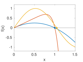
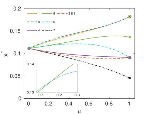
Figure 1: (a): Examples of possible reaction functions to be used in Eqs. (1): $f(x)=x-x^{2}$ in blue, $f(x)=x-x^{10}$ in red and $f(x)=\sin(3x)$ in yellow. (b) A graph of $N=9$ nodes, and (c) the fixed point $\boldsymbol{x^{*}}$ obtained when a reactive random walk model with $f(x)=x-x^{2}$ and different values of the mobility parameter $\mu$ is implemented on such a graph. The inset represents a zoom showing the inversion of $x^{*}_{5}$ and $x^{*}_{6}$ obtained by changing $\mu$.

Limiting case $\mu=0$.    Let us begin the analysis of the reactive random walk model by considering its two limits, namely $\mu=0$ and $\mu=1$. In the first limit, the mobility is completely suppressed and the dynamics of each node is independent of the others. Since we have assumed that the function $f$ is the same for each node, Eqs. (1) reduce to solve the 1-dimensional system $\dot{x}=f(x)$. In principle the reaction function $f$ can be freely chosen among all the functions $f$: $\mathbb{R}\rightarrow\mathbb{R}$. However interesting cases are found when the variable $x(t)$ is bound to converge towards a stationary point, $x^{*}$, defined by $f(x^{*})=0$. The function $f$ should then be chosen among the continuous functions and such that $0$ is included in its image. Moreover, in order to have equilibrium stability, it is necessary that $f$ is monotonically decreasing in, at least, one of the points where it vanishes, in order to ensure that there exists (at least) one stable fixed point $x^{*}$. Some possible examples of reaction functions are reported in Fig. 1.

Limiting case $\mu=1$.    In the opposite limit, when the mobility parameter takes its maximum value $\mu=1$, Eqs. (1) describe a pure random walk process.

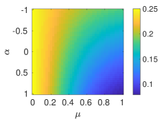
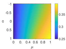
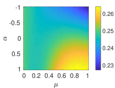
Figure 2: Stationary occupation probability of the nodes of graph in (a) is shown for a reactive random walk as a function of the mobility parameter $\mu$ and of the bias exponent $\alpha$: node 1 (b), node 2 (c), nodes 3 and 4 (d). The latter two nodes yield identical patterns (consequently displayed in just one figure), being symmetric nodes. The same reaction function as in Fig. 1 has been chosen.

The stationary distribution $\boldsymbol{x^{*}}=\{x_{1}^{*},x_{2}^{*},\ldots,x_{N}^{*}\}$ of the dynamics in this limit is obtained by $L^{\rm RW}\boldsymbol{x^{*}}=0$, which is equivalent to $\Pi\boldsymbol{x^{*}}=\boldsymbol{x^{*}}$. The Perron-Frobenius Perron07 ; Frobenius12 theorem ensures that, if the graph is connected and contains at least one odd cycle, the fixed point $\boldsymbol{x^{*}}$ always exists and is unique. In the case of degree-biased random walks we get GomezGardenesLatora08 :

$$x_{i}^{*}=\frac{c_{i}k_{i}^{\alpha}}{\sum_{l}c_{l}k_{l}^{\alpha}}\text{ with }c_{i}=\sum_{j}a_{ij}k_{j}^{\alpha}.$$ (4)

Such an expression, for $\alpha=0$, reduces to $x_{i}^{*}=k_{i}/2K$, meaning that the walker, after a long enough period of time, is found on a node $i$ with a probability linearly proportional to the node degree $k_{i}$. In this case the asymptotic distribution is completely characterized by the degree $\boldsymbol{k}$ of the graph, with better-connected nodes having a larger probability of being visited by the walker.
The general expression for the asymptotic distribution at a node $i$, when $\alpha\neq 0$, depends instead not only on the degree $k_{i}$ of node $i$, but also on the degrees of the first neighbours of node $i$, through the coefficient $c_{i}$, and such dependence can be tuned by changing the value of the exponent $\alpha$. For instance, optimal values of the bias, which depend both on the degree distribution and on the degree-degree correlations of a network, can be found to obtain maximal-entropy random walks  GomezGardenesLatora08 ; Burda09 ; SinatraGomexGardenesLambiotteNicosiaLatora11 or to induce the emergence of synchronization GomezGardenesNicosiaSinatraLatora13 .

The general case.   

The most interesting dynamics of our model emerges at intermediate values of the mobility parameter $\mu$, when interactions at nodes and random movements between nodes are entangled. In this case, the walkers move on the network jumping from node to node, so that the node occupation probability depends on the network connectivity because of the Laplacian contribution but, at the same time, it evolves at each node according to the reaction function. Reaction functions in turn depend on the occupation probability, so that we have different contributions for differently populated node. This leads to a stationary probability $\boldsymbol{x^{*}}$ reflecting the topology of the graph in a way that is non trivial and worth analysing. The stationary probability of the model can be obtained, for any value of $\mu$ in $[0,1]$, by setting $\dot{x}_{i}=0$ in Eqs. (1) and solving numerically the following recursive equations:

$$x_{i}^{*}=\sum_{j}\frac{a_{ij}}{k_{j}}x_{j}^{*}+\frac{(1-\mu)}{\mu}f(x_{i}^{*}).$$ (5)

Notice however that, when $\mu\neq 1$, the state $x_{i}(t)$ of node $i$ in Eqs. (1) is not constrained between 0 and 1. This is an effect caused by the reaction term, which behaves as a source term at each node. If we want to interpret the state of the network as an occupation probability, we need then to further impose the normalization, for instance we can consider the vector $\boldsymbol{x}/\sum_{i}x_{i}$ instead of the vector $\boldsymbol{x}$.

In the following, we will consider a series of examples so as to get a first insight on the properties of the stationary distribution $\boldsymbol{x}^{*}$ for different network structures and for different values of the two main tuning parameters of the model, namely the mobility parameter $\mu$ and the bias exponent $\alpha$.

In Fig. 1, as local interaction, we consider the logistic function $f(x)=x-x^{2}$ shown in panel (a), and we implement the model on the graph of $N=9$ nodes displayed in panel (b). Panel (c) reports the obtained values of the components of the normalized fixed point $\frac{1}{\sum_{i}x_{i}^{*}}(x_{1}^{*},x_{2}^{*},...,x_{9}^{*})$ as functions of the mobility parameter $\mu$, when $\alpha$ is fixed to zero. The numerical results are in agreement with the expected behaviours in the two limiting cases $\mu=0$ and $\mu=1$. In particular, we get $\boldsymbol{x}^{*}=\boldsymbol{k}/2K$ for $\mu=1$, and $\boldsymbol{x}^{*}=\boldsymbol{1}/N$ for $\mu=0$, where $\boldsymbol{1}$ denotes an $N$-dimensional vector with all entries being identically equal to 1. This means that all the curves in the figure start from the same point $\boldsymbol{x}^{*}$ at $\mu=0$, while for $\mu=1$ we observe four different points $\boldsymbol{x}^{*}$. The graph considered has in fact nodes with four different degrees, namely $k=1,2,3$ and 4, and curves corresponding to nodes with same number of links will converge to the same point $x^{*}$ for $\mu=1$. However, at intermediate values of $\mu$, even nodes with the same degree can exhibit different values of $x^{*}$ (with the exception of some of them, see Section V for a discussion on symmetric nodes) going from their degree class at $\mu=1$ towards $1/N$ at $\mu=0$. In particular, the various curves of $x^{*}$ as a function of $\mu$ can cluster in a different way when heading towards the limit $\mu=0$. Let us focus for instance on the behaviour of the node 6 of the graph. Such a node belongs to the degree-2 class but, following the curve of its stationary state when it goes from $\mu=1$ to $\mu=0$, we notice that it separates from the curves of the other nodes of its class, approaching the curve of node 5, $x_{5}^{*}$, although the latter node is characterized by a larger degree ($k_{5}=3$). Moreover, node 6 even overcomes node 5 for small values of $\mu$ before both curve collapse towards the homogeneous solution. The crossing between the two curves is highlighted in the inset of Fig. 1.

In the most general case, in our model it is possible to tune both the local dynamics, by choosing different reaction functions $f(x)$, and the bias in the random walk, by considering values of the exponent $\alpha\neq 0$. An illustrative example is reported in Fig. 2 in the case of a smaller graph with only four nodes. The three coloured panels show the three different values of the fixed point at the nodes of the network as functions of the mobility parameter $\mu$ and the bias exponent $\alpha$. Notice that node 3 and 4 have the same symmetry in the graph, so they reach the same fixed point (see Section V for a discussion of symmetries). In detail, while for $\mu$ and $\alpha$ equal to zero the four nodes exhibit the same value of the occupation probability, $x^{*}_{i}=0.25$ $\forall i$, when we increase the mobility parameter we observe a non-trivial behaviour of these values, which in general decrease for low-degree nodes and increase for high-degree nodes. The effect of introducing a degree-bias in the random walk by turning on and tuning the bias parameter is instead that the occupation probability of the most connected nodes (see nodes 2, 3 and 4) is enhanced for positive and decreased for negative values of $\alpha$. The opposite happens for the less connected nodes (node 1).

Our third and last numerical example is reported in Fig. 3. In this case, we have considered two different topologies, namely a scale-free network with $N=100$ nodes (first row panels) and a smaller network with $N=11$ nodes (second row panels). Again, the stationary occupation probability at the nodes of the graphs is shown for various values of $\mu$. For both networks, the size of the nodes in the graphs is proportional to $\boldsymbol{x^{*}}$, while the four different columns represent respectively the four values of the mobility parameter, $\mu=0.1,0.5,0.9,1$. While all the nodes have almost equal size for small values of $\mu$, they clearly tend to differentiate when $\mu$ increases. Notice that for $\mu=1$ the node size only reflects their degree, so that the nodes with the largest sizes are the hubs of the scale-free network in the first row. For intermediate values of the mobility parameter (see for instance $\mu=0.9$), instead the nodes with the largest occupation probability are those connecting isolated vertices to the rest of the network, irrespective of their own degree. This is evident for the second graph in the second and third rows. For this graph symmetric nodes are also highlighted in figure (see Section V for a formal definition of symmetric nodes) by adopting the same colours for pairs of nodes with the same symmetry, and reporting in gray nodes not having a symmetric counterpart.

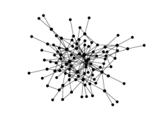
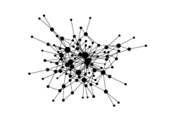
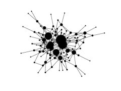
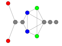
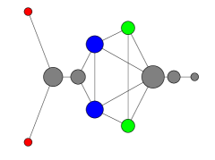
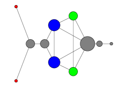
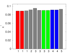
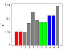
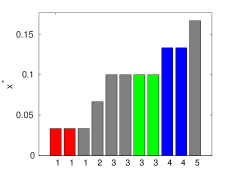
[5pt]$\mu=0.1$ [5pt]$\mu=0.5$ [5pt]$\mu=0.9$ [5pt]$\mu=1$

Figure 3: Reactive random walks on a scale-free network with $p_{k}\simeq k^{-\gamma}$ and $\gamma=2.2$, $N=100$ and mean degree $\langle k\rangle=3.6$, and on a toy graph with only 11 nodes. The four columns represent four different values of the mobility parameter: $\mu=0.1$, $\mu=0.5$, $\mu=0.9$ and $\mu=1$, where the size of the nodes is proportional to the different components of $\boldsymbol{x^{*}}$. The reaction function selected are $f(x)=x-x^{2}$ for the first network, and $f(x)=\sin(3x)$ for the second one. In the second graph, the same colour has been used for nodes with the same symmetry, while colour gray has been used for all other (non-symmetric) nodes. The histograms report the stationary occupation at each node, while the node degree is indicated on the $x$ axis.

III Analytical derivation of the stationary state

The fixed point $\boldsymbol{x}^{*}$ of the reactive random walk model in Eqs. (1) is in general not easy to obtain analytically because of the interplay between random walk dynamics and local interactions. Approximate techniques can be however employed in the low-mobility limit $\mu\simeq 0$, when the local dynamics is only slightly modified by coupling between network nodes due to the movement. In this limit, it is possible to derive a perturbative estimate for $\boldsymbol{x}^{*}$: $\boldsymbol{x}^{*}=s^{*}\boldsymbol{1}+\sum_{n=1}^{\infty}\mu^{n}\boldsymbol{\delta x}^{(n)}$, where $\boldsymbol{\delta x}^{(n)}$ stands for the $n$-th correction to the uncoupled case. The first two corrections take the explicit form:

$$\delta x_{i}^{(1)}=-\frac{s^{*}}{f^{\prime}(s^{*})}\sum_{j}l^{\rm RW}_{ij}$$ (6)

and

$$\begin{split}\delta x_{i}^{(2)}&=-\frac{(s^{*})^{2}}{2}\frac{f^{\prime\prime}(s^{*})}{f^{\prime}(s^{*})^{3}}\biggl{(}\sum_{j}l^{\rm RW}_{ij}\biggr{)}^{2}\\ &-\frac{s^{*}}{f^{\prime}(s^{*})}\sum_{j}l^{\rm RW}_{ij}+\frac{s^{*}}{f^{\prime}(s^{*})^{2}}\sum_{j}l^{\rm RW}_{ij}\sum_{k}l^{\rm RW}_{jk}=\\ &=\delta x^{(1)}_{i}-\frac{f^{\prime\prime}(s^{*})}{2f^{\prime}(s^{*})}(\delta x^{(1)}_{i})^{2}-\frac{1}{f^{\prime}(s^{*})}\sum_{j}l^{\rm RW}_{ij}\delta x^{(1)}_{j}\end{split}$$ (7)

where $s^{*}$ is the solution for $\mu=0$, $f(s^{*})=0$. In figure 4 we show that the analytical predictions are in agreement with the numerical solution. In particular, we consider reactive random walkers with a mobility parameter $\mu=0.1$ and a logistic function as local interaction term, and we implement the model on the graph of collaborations among jazz musicians jazz_net .
If $f$ is a $C^{\infty}$ function, the perturbative terms can be computed for each order $n$. In this case the hypothesis of small $\mu$ can be relaxed and the analytical solution for the fixed point can be, in principle, exactly determined. In such a case, the generic $n$-th correction can be cast in the form:

$$\begin{split}\delta x_{i}^{(n)}=&-\frac{1}{f^{\prime}(s^{*})}\Biggl{\{}\sum_{r=2}^{n}\frac{f^{(r)}}{r!}\Biggl{[}\sum_{m_{1}=1}^{n-r+1}\hskip 5.69054pt\sum_{m_{2}=1}^{n-r-m_{1}+2}\hskip 5.69054pt\sum_{m_{3}=1}^{n-r-m_{1}-m_{2}+3}...\sum_{m_{r-1}=1}^{n-\sum_{j=1}^{r-2}m_{j}-1}\delta x_{i}^{(m_{1})}\delta x_{i}^{(m_{2})}...\delta x_{i}^{(m_{r-1})}\delta x_{i}^{(n-\sum_{k=1}^{r-1}m_{k})}\Biggr{]}\\ &-\sum_{r=2}^{n-1}\frac{f^{(r)}}{r!}\Biggl{[}\sum_{m_{1}=1}^{n-r}\hskip 5.69054pt\sum_{m_{2}=1}^{n-r-m_{1}+1}\hskip 5.69054pt\sum_{m_{3}=1}^{n-r-m_{1}-m_{2}+2}...\sum_{m_{r-1}=1}^{n-\sum_{j=1}^{r-2}m_{j}-2}\delta x_{i}^{(m_{1})}\delta x_{i}^{(m_{2})}...\delta x_{i}^{(m_{r-1})}\delta x_{i}^{(n-1-\sum_{k=1}^{r-1}m_{k})}\Biggr{]}\\ &-f^{\prime}(s^{*})\delta x_{i}^{(n-1)}+\sum_{j}l^{\rm RW}_{ij}\delta x_{j}^{(n-1)}\Biggr{\}}\end{split}$$ (8)

where $f^{(r)}$ is the $r$-th derivative computed in $s^{*}$.
As expected, at different perturbative orders the local dynamics involves successive derivatives of $f$ at $s^{*}$. In particular, the first correction $\boldsymbol{\delta x}^{(1)}$ is only sensitive to the the first derivative, while in $\boldsymbol{\delta x}^{(2)}$ the second derivative appear. In general, the $n$-th correction is characterized by all the derivatives of $f$ until the $n$-th one. More interestingly it is worth noticing that $\delta x^{(1)}_{i}$ contains a term that, when the random walk is unbiased, is proportional to $\sum_{j}a_{ij}/k_{j}$, which essentially is a sum over all neighbours of node $i$ of their inverse degree. This implies that the first correction to the generic $i$-th component of the uniform fixed point depends on the inverse degree of all the nodes of the graph that are adjacent to $i$. In the second order correction, we instead find the term $\sum_{jl}a_{ij}/k_{j}a_{jl}/k_{l}$. The fixed point computed at the second order in $\mu$ thus not only depends on the inverse degree of the nearest neighbours of node $i$, but also on the inverse degree of its second-nearest neighbours. By iterating forward this reasoning, the $n$-th correction will depend on the $n$-th nearest neighbours degrees: the term $\sum_{j}l^{\rm RW}_{ij}\delta x_{j}^{(n-1)}$ in eq. (8) takes recursively into account all the nodes of the network that can be reached, in at most $n$ time steps, when starting from node $i$. Obviously, when $n$ goes to infinity all the nodes of the network contribute with their inverse degree.

It is also worth observing that the perturbative calculation can be readily extended to the general case of biased random walks. To this end one should consider the more general Laplacian form in the last term of each correction: $\sum_{j}l^{\rm RW}_{ij}\delta x_{j}^{(n-1)}$. In this case, the first correction $\delta x_{i}^{(1)}$ is not solely influenced by first neighbours of node $i$, but also depends on the second neighbours, being proportional to $k_{i}^{\alpha}\sum_{j}\frac{a_{ij}}{\sum_{l}a_{lj}k_{l}^{\alpha}}$. Analogously, for the second correction term, the biased random walks introduces a dependency on the neighbours of all nodes at distance two from each vertex, and so on. In general, considering a degree bias always has the effect of moving the set of involved nodes to further proximity level in the network, as already observed in GomezGardenesLatora08 in the case of non-reactive random walks.

In the next three sections we will explore how the occupation probability of reactive random walkers can turn useful to define novel measures of functional centrality for the nodes of a network, to detect network symmetries, or to distinguish assortative from disassortative networks.

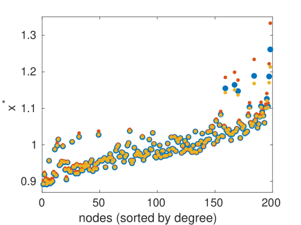
Figure 4: Comparison between analytical predictions (first order in red and second order in yellow) and numerical results (blues dots). The stationary occupation probability of different nodes (sorted by their degree) is shown for reactive random walkers with logistic growth $f(x)=x-x^{2}$ on graph of collaboration among jazz musicians jazz_net . The mobility parameter $\mu$ has been set to 0.1.

IV Measures of functional ranking

Centrality measures allow to rank the nodes according to their location in the network LatoraNicosiaRusso17book . Originally employed in social network analysis to infer the influent actors in a social system, but soon adopted in many other fields, different centrality measures have been constructed to capture different aspects which make a node important, from the number and strength of its connections to its reachability. Commonly used centrality measures are the eigenvector centrality Perron07 ; Frobenius12 , the $\alpha$-centrality Bonacich72 ; BonacichLloyd01 , the betweenness centrality Freeman77 , the closeness centrality Freeman78 and, of course the simplest one, the degree centrality. This latter corresponds to the fixed point of our model in the limit $\mu=1$. In this case, the stationary occupation probability $x^{*}_{i}$ is indeeed proportional to the degree of node $i$. However, in our model of reactive random walkers, when $\mu\neq 1$, the stationary state of the model will also depend on the choice of the local dynamics, resulting in a plethora of distinct configurations fostering different roles within the network. In other words, for a fixed value of the mobility parameter we can interpret our dynamical system as a reaction-dependent centrality measure. Moreover, we note that the form of Eq. (5) on which this centrality measure is based, is reminiscent of other existing definitions of centralities such as a generalization of the Bonacich centrality Bonacich72 known as the $\alpha$-centrality  BonacichLloyd01 , and the PageRank centrality (PRC) BrinPage98 . For instance, the PageRank centrality $x_{i}^{\rm PR}$ of a graph node $i$ is defined as  Langville04 ; Gleich15 ; Bryan06 :

$$x_{i}^{\rm PR}=d\sum_{j}\frac{a_{ij}}{k_{j}}x_{j}^{\rm PR}+\frac{1-d}{N}$$ (9)

where $d\in(0,1)$ is a parameter usually set equal to 0.85. PRC was originally proposed as a method to rank the pages of the World Wide Web. Indeed, it mimics the process of a typical user navigating through the World Wide Web as a special random walk with “teleportation” on the corresponding graph. Such a random walker with a probability $d$ performs local moves on the graph (most of the times a user surfing on the Web randomly click one of the links in the page that is currently being visited), while with a probability $1-d$ starts again the process at a node randomly chosen from the $N$ nodes of the graph (the surfer starts again from a new Web site). The latter action, the so-called “teleportation” is represented by the term $(1-d)/N$ in Eq. (9). Notice that the value of $d=0.85$ is estimated from the average frequency at which surfers recur to their browser’s bookmark feature. The introduction of the teleportation term assigns a uniform non-zero weight to each vertex, and it is particularly useful to avoid pathological cases of nodes with null centrality, in the case the graph is not connected (or strongly connected if a directed graph). In some cases however the teleportation contribution is not uniform, but can be designed to gauge an intrinsinc importance of each node. This implies enforcing a dependence on the generic node index $i$ in the second term in the right hand side of Eq. (9). The advantage of using Eq. (5) instead of Eq. (9) as a measure of centrality then consists in the possibility of freely choosing the reaction term. The adoption of function $f(x_{i})$ in Eq. (5), assigning a different contribute to each node $i$ that depends on $x_{i}$, finds a plausible justification in the fact that the importance of a node may also depend on other factors, not necessarily directly linked to the topology of the graph, such as the status or functionality of the node. In a social network, for instance, this factor could be related to the age, social status or income of an individual. Moreover, $f$ can be chosen so as to take into account the temporal evolution of some features of the nodes of the network. Let us consider again the problem of ranking Web pages. PageRank centrality in Eq. (9) can be modified by replacing the constant teleportation term with a variable contribution, due for instance to the number of visualizations of each page, which could be suitably described by a non-constant term proportional to $x_{i}(t)$, or more generally by a function $f(x_{i})$ as in Eq. (5).

As a practical example let us come back to examining the graph in Fig. 1 and focus again on node 6. According to stardard centrality measures such a node would not result as a very central one, being in a peripheral part of the graph and having just two neighbours. However, one the neighbours is node 7, which is a graph leaf and this makes node 6 its only bridge towards the rest of the graph. This consideration highlights the importance of nodes bridging other nodes of the network and, depending on which characteristics we want to focus on, could be an extremely useful feature to take into account when devising a measure of node centrality. Increasing the importance of this class of nodes can be for instance obtained by an appropriate choice of function $f(x)$ in Eq. (5). This is clearly shown in Fig. 5, where the rankings of the graph nodes obtained for different reference reaction functions and also for different choices of the mobility and bias parameters are compared. The nodes are sorted according to their degree, which is explicitly indicated on the x-axis, while the other reported numbers correspond to node labels as in Fig. 1. Node 6, which bridges node 7 to the rest of the graph, appears to be more sensitive than the others to the changes, with a large variety of ranking positions, especially if compared to the other nodes with the same degree. The magenta and green symbols respectively refer to a positive ($\alpha=1$) and a negative ($\alpha=-1$) bias with $f(x)=x-x^{2}$ and $\mu=0.85$. We observe that it is also possible to reproduce the same trend of the PRC (red symbols) by again using the logistic function with the same value of the mobility parameter, but setting the bias to zero (black symbols). A different reaction is used for the blue curve: $f(x)=x-x^{10}$ with $\mu=0.7$ and $\alpha=0$.
The same types of functional ranking as in Fig. 5 have also been adopted in Fig. 5 for the nodes of the network of collaborations among jazz musicians, and the results are reported with the same color code. A similar general trend appears, with low degree nodes enhanced by a negative degree bias and vice versa hubs enhanced by a positive bias. In addition to this, we observe some fluctuations with peaks appearing in the different ranking measures, most of them corresponding to nodes bridging one or more otherwise isolated nodes of the network.

In conclusion, the proposed measure of functional ranking can mimic other centrality measures, like PRC, in the limit of large $\mu$, where diffusion is important and it is only slightly modified by the local interactions. In general, for every value of $\mu$ between 0 and 1, our model of reactive random walkers can be thought as a new way to measure centrality which accounts for the differences between nodes at a deeper level, with the focus on different time-varying characteristics of the nodes themselves.

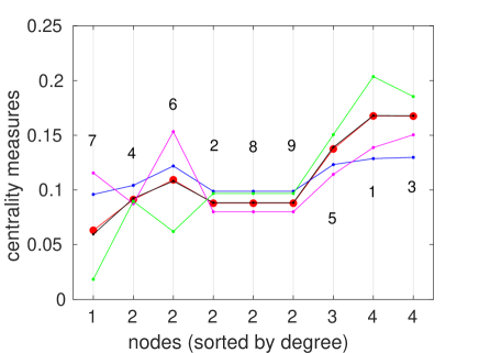
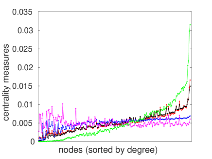
Figure 5: Measures of centrality based on Eq. (5) and on different choices of $f$ and $\alpha$ are compared to PRC (red curves) in the case of two networks, the graph of $N=9$ nodes in Fig. 1 and the graph of $N=198$ nodes representing the jazz musicians network jazz_net .

V Detecting network symmetries

Symmetries are ubiquitous in nature, and one of the main reasons by which humans have been long attempted to describe and model the world through the tools and the language of mathematics. In complex networks, despite the fact that symmetric nodes may appear as special cases, they are surprisingly numerous in real and artificial network structures SiddiquePecoraSorrentino17 .

In mathematical terms, network symmetries form a group, each element of which can be described by a permutation matrix that re-orders the nodes in a way that leaves the graph unchanged. More precisely, a graph $G$ with $N$ nodes described by the adjacency matrix $A$ has a symmetry if there exists a permutation matrix $P$, i.e. a $N\times N$ matrix with each row and each column having exactly one entry equal to 1 and all others 0, such that $P$ commutes with $A$: $PA=AP$. This is equivalent to say that $PAP^{-1}=A$, namely that $PAP^{-1}$ performs a relabeling of the nodes of the original graph which preserves the adjacency matrix $A$. Therefore, two nodes of the graph are said symmetric if their swapping preserves the adjacency relation. This implies that two symmetric nodes are necessarily characterized by the same degree, but also that their neighbours must have the same degree, so as the neighbours of their neighbours, and so on.

While network symmetries may be easy to spot in small graphs like those considered in Fig. 1 and in Fig. 3, this is typically not the case for large graphs. Different techniques to reveal symmetries in networks have been developed, both numerical and analytical Nicosia_etal13 ; PecoraSorrentino_etal14 ; SiddiquePecoraSorrentino17 ; ZhangMotterNishikawa17 . As we will show below, reactive random walkers provide another method to detect symmetric nodes by looking at the value of the stationary occupation probability at different nodes. In fact, while in the case $\mu=1$ of a pure random walk process the fixed point $\boldsymbol{x}^{*}$ is solely determined by the node degrees, when $\mu\neq 1$ the dynamics is governed by the network as a whole and the value of the stationary occupation probability at a node will depend of its degree, but also on the properties of the second, third and so on neighbours. Hence, it is plausible to conclude that only perfectly symmetric nodes can assume the same asymptotic occupation probability, and to propose to detect symmetric nodes of a graph by looking at those having the same value of $\boldsymbol{x}^{*}$ for a reactive random walker model with $\mu\neq 1$ on the graph.

An analytical argument in support of this can be obtained from the perturbative derivation of the stationary state presented in Section III. In the limit $\mu\simeq 0$, the expression for the first correction $\delta x^{(1)}_{i}$ to the uniform stationary state given in Eq. (6) contains a term proportional to $\sum_{j}a_{ij}/k_{j}$, which indicates the dependence of the stationary state on the degree of the neighbours of $i$. Analogously, the degree of the second nearest neighbours can be found in the second correction $\delta x^{(2)}_{i}$ , while the degree of the $n$-th nearest neighbours appears in the $n$-th correction. The value of $x^{*}_{i}$ of a node $i$ will consequently depend on the degrees of all the nodes in the graph. Since two symmetric nodes share the same connectivity at each level of neighbourhood, we can then find symmetric nodes as those with exactly the same value of $x^{*}$.

Let us come back to the graphs considered in Figs. 1 and 3. In the first example the three nodes labeled as 2, 8 and 9 are symmetric, as can be seen directly from figure 1 (b), given that they share the same set of neighbours. The existence of such a symmetry is also revealed by looking at the behaviour of the occupation probability of different nodes when varying $\mu$: Fig. 1(b) shows that the curves corresponding to these three nodes are indistinguishable. Another remarkable example is reported in Fig. 3, where the graph reported in the second row panels is taken as reference model to observe the variation in the occupation probability state for different values of $\mu$. Here, nodes with the same symmetries are shown with the same colour, while the remaining nodes are in grey, and correspond to exactly the same value of $\boldsymbol{x}$, as reported in the third row panels of the same figure.

A more general argument that extends the results above from $\mu\simeq 0$ to the general case $\mu\neq 1$ can be obtained by proving that Eqs. (1) are equivariant under a permutation of symmetric nodes PecoraSorrentino_etal14 . Such equations can be rewritten in vectorial notation as:

$$\boldsymbol{\dot{x}}=AK^{-1}\boldsymbol{x}-\boldsymbol{x}+\mathcal{F}(\boldsymbol{x})$$ (10)

where $K=\{k_{ij}\}$ is a diagonal matrix whose entries are defined as $k_{ij}=k_{i}\delta_{ij}$, and the functional $\mathcal{F}:\mathbb{R}^{N}\rightarrow\mathbb{R}^{N}$ is defined such that the generic $i$-th element of the image vector $[\mathcal{F}(\boldsymbol{x})]_{i}$ is equal to $f(x_{i})$. Our goal is now to prove that Eq. (10) also holds for the permuted vector $P\boldsymbol{x}$. Left-multiplying the equation by matrix $P$ we get:

$$P\boldsymbol{\dot{x}} = PAK^{-1}\boldsymbol{x}-P\boldsymbol{x}+P\mathcal{F}(\boldsymbol{x})=$$ (11)

$$= AK^{-1}P\boldsymbol{x}-P\boldsymbol{x}+P\mathcal{F}(\boldsymbol{x})$$

where in the last equality we have used the fact that $P$ commutes with $A$ and, since symmetric nodes have the same degree, it also commutes with $K$ and consequently with its inverse. Now we observe that the role of matrix $P$ is to permute symmetric nodes leaving the others unchanged. The effect of $P$ on a generic vector $\boldsymbol{v}\in\mathbb{R}^{N}$ is $[P\boldsymbol{v}]_{i}=v_{\tilde{i}}$ where $\tilde{i}$ denotes the node of the network which is the symmetric twin of $i$, if it exists, otherwise $\tilde{i}=i$. Consequently, when we apply $P$ to $\mathcal{F}(\boldsymbol{x})$ we obtain a vector whose $i$-th component is:

$$[P\mathcal{F}(\boldsymbol{x})]_{i}=[\mathcal{F}(\boldsymbol{x})]_{\tilde{i}}=f(x_{\tilde{i}})=f([P\boldsymbol{x}]_{i})=[\mathcal{F}(P\boldsymbol{x})]_{i}$$ (12)

Making use of this result, Eq. (11) becomes the equivalent of Eq. (10) evaluated for $P\boldsymbol{x}$ instead of $\boldsymbol{x}$, which is what we wanted to prove.

VI Measuring degree correlations

A distinguishing feature of many real-world networks is the presence of non-trivial patterns of degree-degree correlations  PastorSatorrasVazquezVespignani01 ; Newman02 ; Newman03 . In the case of positive degree-degree correlation the network is said to be assortative: this is often the case for social networks, where hubs have a pronounced tendency to be linked to each other. Conversely, a network is said disassortative if the correlations are negative and connections between hubs and poorly connected nodes are favored. Well-known examples of disassortative networks are the Internet, and biological networks such as protein-protein interaction networks, where high degree nodes tend to avoid each other.

One possible way to reveal the presence of degree-degree correlations in a network is to compute the average degree of neighbours of nodes of degree $k$, and to look at how this quantity depends on the value of $k$. The average degree $k_{nn,i}$ of the neighbours of node $i$ is defined as $k_{nn,i}=\frac{1}{k_{i}}\sum_{j}a_{ij}k_{j}$. To obtain the average degree of neighbours of nodes of degree $k$, we need to average the quantity $k_{nn,i}$ over all nodes $i$ of degree $k$. Let us denote as $p_{k^{\prime}|k}$ the conditional probability that a link from a node of degree $k$ is connected to a node of degree $k^{\prime}$. Now, by expressing the sum over nodes as a sum over degree classes, the average degree of the nearest neighbours of nodes with a given degree $k$ can be written as:

$$\langle k_{nn}\rangle_{k}=\sum_{k^{\prime}}k^{\prime}p_{k^{\prime}|k}.$$

The function $\langle k_{nn}\rangle_{k}$ is a good indicator of the presence of degree correlations in a network. In fact, the quantity $\langle k_{nn}\rangle_{k}$ increases with $k$ when the network has positive degree correlations, it is decreasing when the network has negative correlations, while it is constant and equal to $\langle k^{2}\rangle/\langle k\rangle$ for uncorrelated networks.
We will now show that the dynamics of the reactive random walker model of Eq. (1) is sensitive to the presence of correlations in the the underlying network, and it is therefore possible to detect and measure the assortative or disassortative nature of a network from the asymptotic node occupation probability. To this end we need to return to the perturbative approach to obtain the equilibrium occupation probability discussed in Section III. As already remarked, a full hierarchy of terms are found to appear as a byproduct of the calculation, which respectively relate to paths connecting nodes that are $1,2,3,\ldots$ steps away from any selected node. Let us focus on the first correction to the uniform state, namely the term $\delta x^{(1)}_{i}$, as specified in Eq. (6). Up to the multiplicative node-invariant factor $s^{*}/f^{\prime}(s^{*})$, $\delta x^{(1)}_{i}$ is equal to $\sum_{j}l^{\rm RW}_{ij}=\sum_{j}{a_{ij}}/{k_{j}}-1$. Therefore, at the first order, the difference between the equilibrium distribution and the uniform state is governed by the quantity:

$$w_{i}^{(1)}\equiv\sum_{j=1}^{N}\frac{a_{ij}}{k_{j}}={k_{i}}{\langle\frac{1}{k_{nn}}\rangle},$$ (13)

representing, for a generic node $i$, the sum of the inverse degrees of all its neighbours. The quantity $w_{i}^{(1)}$ is always non-negative, and it gets larger when many nodes are adjacent to node $i$ (large degree $k_{i}$, corresponding to many terms in the sum) and all such nodes display smaller degrees. In the particular case in which all the nodes connected to $i$ have exactly degree equal to $k_{i}$, we get $w_{i}^{(1)}=1$. When instead, the degree $k_{i}$ of node $i$ is smaller than the inverse of the mean inverse degree of the nodes adjacent to $i$ , then we have $0<w_{i}^{(1)}<1$. In the extreme case of low degree nodes connected to hubs $w_{i}^{(1)}$ tends to zero.

Looking at the whole network, the vector $\boldsymbol{w}$ can be turned into an effective indicator for the presence of degree-degree correlations that relies on the harmonic mean of the degrees instead that on the standard mean.

For instance, we can consider the average value of $w_{i}^{(1)}$ for all nodes $i$ of degree $k_{i}=k$. Such a quantity can be written in terms of the adjacency matrix of the graph as:

$$\langle w^{(1)}\rangle_{k}=\frac{1}{N_{k}}\sum_{i=1}^{N}\sum_{j=1}^{N}\frac{a_{ij}}{k_{j}}\delta_{k_{i},k}$$ (14)

where $N_{k}=\sum_{i=1}^{N}\delta_{k_{i},k}$ is the number of nodes of degree $k$. We can rewrite the previous equation by making use of the conditional probability $p_{k^{\prime}|k}$, so that the sum over all neighbours $j$ of $i$ becomes a sum over the degrees $k^{\prime}$ of the nodes adjacent to those of degree $k$. We finally obtain:

$$\langle w^{(1)}\rangle_{k}=k\sum_{k^{\prime}}\frac{1}{k^{\prime}}p_{k^{\prime}|k}=k\langle\frac{1}{k^{\prime}}\rangle_{k},$$ (15)

where the quantity $\langle{1}/{k^{\prime}}\rangle_{k}$ denotes the average of the inverse degree of the first neighbours of nodes of degree $k$. In absence of degree correlations the conditional probability takes the form: $p_{k^{\prime}|k}^{\rm nc}={k^{\prime}p_{k^{\prime}}}/{\langle k\rangle}$  Newman02 ; LatoraNicosiaRusso17book , where $p_{k}$ is the degree distribution of the network, $\langle k\rangle$ is the average degree, and “nc” stands for no correlations. Hence, in uncorrelated networks the quantity in Eq. (15) reduces to:

$$\langle w^{(1)}_{\rm nc}\rangle_{k}=\bigl{(}k\sum_{k^{\prime}}\frac{1}{k^{\prime}}p_{k^{\prime}|k}^{\rm nc}\bigr{)}=\frac{k}{\langle k\rangle}$$ (16)

and is a linearly increasing function of $k$ with slope equal to $1/\langle k\rangle$. Such a function represents the reference case to compare to when evaluating the quantity $\langle w^{(1)}\rangle_{k}$ for a given network.

In Fig. 6(a) we plot $\langle w^{(1)}\rangle_{k}$ as a function of $k$ for three synthetic networks, respectively with positive, negative and no degree correlations. The uncorrelated network is an Erdős-Rényi random graph with $N=1000$ nodes and $K=10000$ edges, while the other two have been generated from the uncorrelated one by using an algorithm that swaps edges according to the degree of the corresponding nodes BonaventuraNicosiaLatora14 ; XulviBrunetSokolov05 , to produce respectively a disassortative graph with correlation coefficient $r=-0.94$ and an assortative graph with $r=0.93$ and  Newman02 . The algorithm preserves not only the average degree $\langle k\rangle$, but also the entire degree distribution, which is shown in lower-right inset. Consequently, the results for the three networks, shown respectively as purple, yellow and red pluses, can be directly compared to the same analytical prediction $\langle w^{(1)}_{\rm nc}\rangle_{k}$ (straight line), which is clearly well in agreement with the randomized network. In the disassortative graph we observe that the quantity $\langle w^{(1)}\rangle_{k}$ is larger than $\langle w_{\rm nc}\rangle_{k}$ for degree values $k>\langle k\rangle$. This is because the first neighbours of the hubs are typically poorly connected, i.e. $\langle 1/k^{\prime}\rangle_{k}>1/\langle k\rangle$ when $k>\langle k\rangle$. Conversely, $\langle w^{(1)}\rangle_{k}$ is smaller than $\langle w^{(1)}_{\rm nc}\rangle_{k}$ for poorly connected nodes, i.e. for $k<\langle k\rangle$. In the assortative graph, as expected, $\langle w\rangle_{k}\simeq 1$ for most of the degree classes. Deviations from perfect assortativity only occur at the two extremes of the degree distribution, i.e. for limit values of the degree: a sample node with low (high) degree is in fact linked to nodes whose degree is in average larger (lower) than its own.

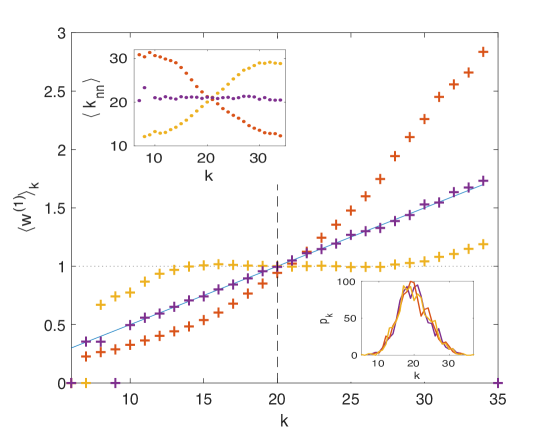
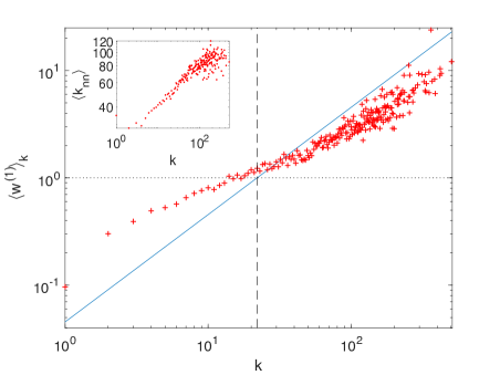
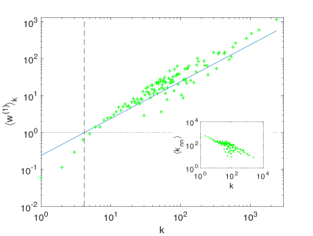
Figure 6: The quantity $\langle w^{(1)}\rangle_{k}$ is reported as a function of $k$ for (a) three synthetic graphs with the same number of nodes and links, and respectively disassortative ($r=-0.94$, red pluses), assortative ($r=0.93$, yellow pluses) and uncorrelated ($r\sim 0$, purple pluses). The vertical dashed line identifies the mean degree $\langle k\rangle$. The mean degree $\langle k_{nn}\rangle_{k}$ of the nearest neighbours of nodes of degree $k$ is displayed in the upper-left inset, while the degree distribution $p_{k}$ is shown in the lower-right inset. Same quantities as in panel (a) for two real networks: (b) the network of collaborations in astrophysics and (c) Internet AS. Double-logarithmic scales have been used.

In Fig. 6(b) and (c) we show the results obtained for two real-world networks with known mixing patterns, namely the collaboration networks of astrophysicists Newman01 and the Internet at the autonomous systems (AS) level  PastorSatorrasVazquezVespignani01 . The first network has $N=17903$, an average degree $\langle k\rangle$ equal to 22.2 and is assortative with correlation coefficient $r=0.23$, while the second one has $N=11174$, $\langle k\rangle=4.3$ and is disassortative with $r=-0.19$. A logarithmic scale has been adopted in the two plots, as both networks exhibit long-tailed degree distributions. The plots show larger fluctuations that those observed for the artificially generated graphs. The general behaviour is however preserved and allows to identify the two different types of degree-degree correlations. In particular, the inversion of the trend, which occurs around the mean degree, is clearly preserved. For the assortative network of collaborations in astrophysics $\langle w^{(1)}\rangle$ is larger than the value expected for the uncorrelated case when $k<\langle k\rangle$, while it is smaller that this for almost all the larger values of $k$. The opposite behaviour is displayed by the Internet network, which is instead disassortative. A possible way to detect the sign and, at the same time, to quantify the entity of the correlations in a network from the study of the quantity $\langle w^{(1)}\rangle_{k}$ is to extract the slope of the curve $\langle w^{(1)}\rangle_{k}$ as a function of $k$ at point $k=\langle k\rangle$, and compare it to the slope of $\langle w^{(1)}_{\rm nc}\rangle_{k}$ vs $k$ for the corresponding randomized case. For instance, we can evaluate the difference $\cal S$ between the two slopes multiplied by $\langle k\rangle$:

$${\cal S} = \langle k\rangle\frac{d}{dk}\Bigl{(}\langle w^{(1)}_{\rm nc}\rangle_{k}-\langle w^{(1)}\rangle_{k}\Bigr{)}\Big{|}_{k=\langle k\rangle}=$$ (17)

$$= 1-\langle k\rangle\frac{d}{dk}\biggl{(}k\sum_{k^{\prime}}\frac{1}{k^{\prime}}p_{k^{\prime}|k}\biggr{)}\Bigg{|}_{k=\langle k\rangle}$$

that we name slope variation. The multiplying mean degree has the role of rescaling $\cal S$, which becomes a quantity of order 1 (instead of $1/\langle k\rangle$) and consequently a comparable measure for networks with different connectivity. Such a quantity has been computed for the networks analysed in Fig. 6. Results are reported in Table 1 and compared to the standard quantities usually adopted, namely the Pearson correlation coefficient $r$ and the exponent $\nu$ governing the behaviour, $\langle k_{nn}\rangle_{k}\sim k^{\nu}$, of the average degree of first neighbours of nodes of degree $k$ as a function of $k$. We notice that positive values of the slope variation $\cal S$ are associated to assortative networks, while negative slope differences indicate disassortative ones, in agreement with the standard indicators of degree-degree correlations.

Table 1 also reports the values of $\cal S$ obtained in a sample of other artificial and real-world networks, and shows that the proposed indicator agrees not only for the sign but also for the order of magnitude with the standard measures, when evaluated for networks with strong degree-degree correlations, namely the network of collaboration in Astrophysics, Internet AS and Caida, as well as for artificial networks. The exceptional cases where the value of $\cal S$ results considerably different from $r$ and $\nu$ are those where the degree correlation does not prove to be clearly defined, corresponding to a significant error $\Delta\nu$ obtained from the fit of $k_{nn}(k)$.

In summary the value of $\cal S$ provides indication on the presence of degree-degree correlations that are in all similar to $r$ or $\nu$. However, as the $n$-th term of the expression of $\boldsymbol{x}^{*}$ in Eq. (8) takes into account the degree correlations of a node to those which are $n$ steps away, our indicator can be easily generalized and employed to detect higher order degree correlations. Let us consider for instance the second term $\delta x_{i}^{(2)}$ of the Taylor expansion in Eq.(7). A second order analogue of $w_{i}^{(1)}$ can be defined as $w_{i}^{(2)}\equiv\sum_{jl}\frac{a_{ij}}{k_{j}}\frac{a_{jl}}{k_{l}}$ to measure the inverse degree of the second neighbours of node $i$. Such a quantity represents a measure of the connectivity of node $i$ compared to that of nodes which are two steps away from it. The degree $k_{j}$ present at the denominator mitigates the impact of the number of nodes adjacent to $i$, so that the comparison only takes into account $k_{i}$ and the degree of the second neighbours. Indeed, we have $w_{i}^{(2)}=1$ when all the second neighbours $l$ of $i$ have degree $k_{l}=k_{i}$. As for the case of $w_{i}^{(1)}$, we can consider the average value of $w_{i}^{(2)}$ over all nodes $i$ of degree $k_{i}=k$. Writing this as a summation over degree classes, we have:

$$\langle w^{(2)}\rangle_{k}=\frac{1}{N_{k}}\sum_{i=1}^{N}w_{i}^{(2)}\delta_{k_{i},k}=k\sum_{k^{\prime},k^{\prime\prime}}\frac{1}{k^{\prime\prime}}p_{k^{\prime}|k}p_{k^{\prime\prime}|k^{\prime}}$$ (18)

where $k^{\prime\prime}$ represents the degree of second neighbours. It is important to notice that the above introduced quantity does not measure genuine second order degree correlations in a network but rather how the effect of first order degree correlations reflects on nodes which are at distance of two steps. The generalization to higher orders follows naturally. Assessing the efficacy of this latter quantity as compared to other possible generalization of standard degree correlation measures to higher order Allenperkins17 is left as a challenge for future investigations.

Networks	$N$	$\langle k\rangle$	$r$	$\nu\pm\Delta\nu$	${\cal S}$
Synthetic uncorrelated	1000	20	-0.003	-0.02 $\pm$ 0.01	-0.01
Synthetic assortative	1000	20	0.93	0.83 $\pm$ 0.08	1.02
	1000	20	0.71	0.61 $\pm$ 0.06	0.83
	1000	20	0.50	0.34 $\pm$ 0.05	0.59
	1000	20	0.30	0.19 $\pm$ 0.03	0.36
Synthetic disassortative	1000	20	-0.94	-0.89 $\pm$ 0.07	-0.86
	1000	20	-0.71	-0.66 $\pm$ 0.05	-0.74
	1000	20	-0.50	-0.35 $\pm$ 0.04	-0.52
	1000	20	-0.30	-0.23 $\pm$ 0.02	-0.32
Astrophysics collaboration Newman01	17903	22.01	0.23	0.22 $\pm$ 0.02	0.41
Facebook LeskovecMcauley12	4039	43.69	0.11	0.054$\pm$ 0.051	0.40
Jazz collaborationjazz_net	198	27.70	0.03	0.11$\pm$ 0.04	0.46
Email URV Guimera_etal03	1134	9.61	0.078	0.05 $\pm$ 0.03	0.03
C. elegans frontalKaiserHilgetag06	453	8.97	0.035	0.062 $\pm$ 0.050	0.28
Internet AS PastorSatorrasVazquezVespignani01	11174	4.19	-0.19	-0.52 $\pm$ 0.04	-0.33
Caida Leskovec_etal07	26475	4.03	-0.19	-0.52 $\pm$ 0.03	-0.38
US politics booksKrebs	105	8.42	-0.019	-0.13 $\pm$ 0.07	-0.045
US power grid WattsStrogatz98	4941	2.67	0.003	-0.035 $\pm$ 0.10	-0.18

Table 1: Pearson correlation coefficient $r$, exponent $\nu$ and slope variation $\cal S$ for different synthetic and real-world networks with $N$ nodes and average degree $\langle k\rangle$. The highlighted rows correspond to the three artificial networks analysed in figure 6.

VII Conclusions

Random walks have been extensively used to explore complex networks with the aim of characterizing their structural features and unveil their functional properties. In this article we have introduced a class of random walkers that is subject to node dependent reaction terms. Our model of reactive random walks is formulated in such a way that the relative contribution of the interaction term at the nodes and of the relocation term can be tuned at will, and this improves the sensitivity of the walkers to the structure of the network. In particular, the occupation probability of a given node is shaped by the non trivial interplay between the connectivity patterns and the local interaction functions. We have shown this by determining analytically the asymptotic occupation probability via a perturbative approach that takes a purely reactive dynamics as reference point. Exploiting the dependence of the occupation probabilities on the two tuning parameters of the model, namely the mobility parameter $\mu$ and the bias parameter $\alpha$, and on the shape of the local reaction functions, we have shown that reactive random walkers can turn useful in many different ways. We have first discussed how, by properly adjusting the reaction contribution, one can emphasize nodes bridging otherwise disconnected parts of the network, so that reactive random walkers can readily lead to generalized definitions of node centrality measures. Furthermore, with the help of general arguments and of a series of worked examples we have shown that, by making the random walkers reactive and inspecting their associated density distribution, one can easily detect the symmetries of a network. Finally, the specific form of the perturbative solution has inspired the introduction of a novel indicator for the presence, sign and entity of degree-degree correlations, which differently from other standard measures is based on harmonic averages. We have illustrated how reactive random walkers can distinguish assortative from disassortative networks. The approach can in principle be generalized to include next-to-leading correlations and this defines an intriguing avenue for the investigation of higher-correlation in complex networks which is left for future work.

In conclusion, we hope that this article has proven the versatility and potential of reactive random walkers and that our work will trigger further investigation of the model we have proposed and of its many possible variations.

Appendix

Random walks on networks

Random walks on networks are generally introduced as a discrete time process governed by the equations

$$x_{i}(n+1)=\sum_{j}\pi_{ij}x_{j}(n)$$ (19)

where $x_{i}(n)$ denotes the probability that node $i$ is visited at time step $n$. The stationary distribution $\boldsymbol{x}^{*}=\lim_{n\rightarrow\infty}\boldsymbol{x}(n)$ satisfies the equation $\boldsymbol{x^{*}}=\Pi\boldsymbol{x^{*}}$ and, for undirected networks $\pi_{ij}x_{j}^{*}=\pi_{ji}x_{i}^{*}$, meaning that the flow of probability in each direction must equal each other at equilibrium (detailed balance) Sethna06 . This implies that, if $\pi_{ij}=a_{ij}/k_{j}$, the stationary distribution is proportional to the degree of nodes: $x_{i}^{*}=k_{i}/2K$.
Switching from discrete to continuous time when the spatial support is discrete, as in the case of a network, is not trivial. The main point is to set the time scale which is no longer simply defined by the discrete steps. Two different types of continuous-time random walks can be defined: node-centric and edge-centric  MasudaPorterLambiotte17 . In the node-centric version we consider that a walker sitting on a node waits until the next move for a time $\tau$, where $\tau$ is a random variable. If we assume that there are independent, identical Poisson processes at each node of the graph such that the walkers jump at a constant rate, the corresponding continuous-time process is governed by:

$$\dot{x}_{i}=\sum_{j}(\pi_{ij}-\delta_{ij})x_{j}\equiv\sum_{j}l^{\rm RW}_{ij}x_{j}.$$

where $L^{\rm RW}=\{l^{\rm RW}_{ij}\}$, with $l^{\rm RW}_{ij}=\pi_{ij}-\delta_{ij}$ is the random walk Laplacian. The stationary state is then obtained by setting $\dot{x}_{i}$ equal to zero, which gives $\sum_{j}l^{\rm RW}_{ij}x_{j}^{*}=0$, so yielding the same stationary point of the discrete time version. This also corresponds to the eigenvector of matrix $L^{\rm RW}$ associated to eigenvalue $0$.
In the other type of random walk, the edge-centric, which is also generally called diffusion or fluid model  AldousFill02 ; Samukhin_etal08 ; HoffmanPorterLambiotte12 , a step occurs when the walker decides to move to another node by using one of the outbound edges of its vertex, or in other words, when an edge is activated. Clearly, the more connected is the starting node the larger the set of options that can be alternatively selected to jump away. The walker therefore leaves a node with large degree more quickly than a node with small degree, and the transition rate for a walker starting from node $i$ is equal to $k_{i}$. The occupation probability evolves in this case according to:

$$\dot{x}_{i}=\sum_{j}(a_{ij}-k_{j}\delta_{ij})x_{j}\equiv\sum_{j}l^{\rm Diff}_{ij}x_{j}$$

which defines another Laplacian operator, $L^{\rm Diff}=\{l^{\rm Diff}_{ij}\}$, with $l^{\rm Diff}_{ij}=a_{ij}-k_{j}\delta_{ij}$, associated to diffusion. The stationary distribution $\boldsymbol{x}^{*}$ is in this case homogeneous (as one would expect in a fluid model), being the normalized eigenvector of $L^{\rm Diff}$ associated to 0 an $N$-dimensional vector with all entries $1/N$.

References

- (1) M. E. J. Newman, Networks: An Introduction. Oxford: Oxford University Press, 2010.
- (2) V. Latora, V. Nicosia, and G. Russo, Complex networks: principles, methods and applications. Cambridge University Press, 2017.
- (3) A. Barrat, M. Barthelemy, and A. Vespignani, Dynamical processes on complex networks. Cambridge University Press, 2008.
- (4) X.-Q. Cheng and H.-W. Shen, “Uncovering the community structure associated with the diffusion dynamics on networks,” Journal of Statistical Mechanics: Theory and Experiment, vol. 2010, no. 04, p. P04024, 2010.
- (5) M. De Domenico, “Diffusion geometry unravels the emergence of functional clusters in collective phenomena,” Physical review letters, vol. 118, no. 16, p. 168301, 2017.
- (6) M. Asllani, T. Carletti, F. Di Patti, D. Fanelli, and F. Piazza, “Hopping in the crowd to unveil network topology,” Phys. Rev. Lett., vol. 120, p. 158301, Apr 2018.
- (7) K. Pearson, “The problem of the random walk,” Nature, vol. 72, no. 1867, p. 342, 1905.
- (8) D. Aldous and J. Fill, “Reversible markov chains and random walks on graphs,” 2002.
- (9) J. D. Noh and H. Rieger, “Random walks on complex networks,” Physical review letters, vol. 92, no. 11, p. 118701, 2004.
- (10) S.-J. Yang, “Exploring complex networks by walking on them,” Physical Review E, vol. 71, no. 1, p. 016107, 2005.
- (11) J. Gómez-Gardeñes and V. Latora, “Entropy rate of diffusion processes on complex networks,” Physical Review E, vol. 78, no. 6, p. 065102, 2008.
- (12) Y. Lin and Z. Zhang, “Mean first-passage time for maximal-entropy random walks in complex networks,” Scientific reports, vol. 4, p. 5365, 2014.
- (13) S. Brin and L. Page, “The anatomy of a large-scale hypertextual web search engine,” Computer networks and ISDN systems, vol. 30, no. 1-7, pp. 107–117, 1998.
- (14) P. Bonacich, “Factoring and weighting approaches to status scores and clique identification,” Journal of mathematical sociology, vol. 2, no. 1, pp. 113–120, 1972.
- (15) K. Klemm, M. Á. Serrano, V. M. Eguíluz, and M. San Miguel, “A measure of individual role in collective dynamics,” Scientific reports, vol. 2, p. 292, 2012.
- (16) F. Iannelli, M. S. Mariani, and I. M. Sokolov, “Network centrality based on reaction-diffusion dynamics reveals influential spreaders,” arXiv preprint arXiv:1803.01212, 2018.
- (17) M. Rosvall and C. T. Bergstrom, “Maps of random walks on complex networks reveal community structure,” Proceedings of the National Academy of Sciences, vol. 105, no. 4, pp. 1118–1123, 2008.
- (18) N. Djurdjevac, S. Bruckner, T. Conrad, and C. Schütte, “Random walks on complex modular networks,” Journal of Numerical Analysis, Industrial and Applied Mathematics, vol. 6, no. 1-2, pp. 29 – 50, 2012.
- (19) M. Sarich, N. D. Conrad, S. Bruckner, T. Conrad, and C. Schütte, “Modularity revisited: A novel dynamics-based concept for decomposing complex networks,” Journal of Computational Dynamics, vol. 1, p. 191, 2014.
- (20) L. Peel, J.-C. Delvenne, and R. Lambiotte, “Multiscale mixing patterns in networks,” Proceedings of the National Academy of Sciences, 2018.
- (21) F. Iannelli, A. Koher, D. Brockmann, P. Hövel, and I. M. Sokolov, “Effective distances for epidemics spreading on complex networks,” Physical Review E, vol. 95, no. 1, p. 012313, 2017.
- (22) E. M. Azoff, Neural network time series forecasting of financial markets. John Wiley & Sons, Inc., 1994.
- (23) X.-J. Wang, “Probabilistic decision making by slow reverberation in cortical circuits,” Neuron, vol. 36, no. 5, pp. 955–968, 2002.
- (24) J. E. Kamienkowski, H. Pashler, S. Dehaene, and M. Sigman, “Effects of practice on task architecture: Combined evidence from interference experiments and random-walk models of decision making,” Cognition, vol. 119, no. 1, pp. 81–95, 2011.
- (25) P. Schippers, J. Verboom, J. Knaapen, and R. v. Apeldoorn, “Dispersal and habitat connectivity in complex heterogeneous landscapes: an analysis with a gis-based random walk model,” Ecography, vol. 19, no. 2, pp. 97–106, 1996.
- (26) I. Iacopini, S. c. v. Milojević, and V. Latora, “Network dynamics of innovation processes,” Phys. Rev. Lett., vol. 120, p. 048301, Jan 2018.
- (27) N. D. Conrad, L. Helfmann, J. Zonker, S. Winkelmann, and C. Schütte, “Human mobility and innovation spreading in ancient times: a stochastic agent-based simulation approach,” EPJ Data Science, vol. 7, no. 1, p. 24, 2018.
- (28) R. Levins, “Some demographic and genetic consequences of environmental heterogeneity for biological control,” American Entomologist, vol. 15, no. 3, pp. 237–240, 1969.
- (29) I. Hanski, “Metapopulation dynamics,” Nature, vol. 396, no. 6706, p. 41, 1998.
- (30) O. Ovaskainen and I. Hanski, “Spatially structured metapopulation models: Global and local assessment of metapopulation capacity,” Theoretical Population Biology, vol. 60, no. 4, pp. 281 – 302, 2001.
- (31) D. Urban and T. Keitt, “Landscape connectivity: a graph-theoretic perspective,” Ecology, vol. 82, no. 5, pp. 1205–1218, 2001.
- (32) V. Nicosia, F. Bagnoli, and V. Latora, “Impact of network structure on a model of diffusion and competitive interaction,” EPL (Europhysics Letters), vol. 94, no. 6, p. 68009, 2011.
- (33) G. Cencetti, F. Bagnoli, F. Di Patti, and D. Fanelli, “The second will be first: competition on directed networks,” Scientific Reports, vol. 6, no. 27116, 2015.
- (34) M. Bonaventura, V. Nicosia, and V. Latora, “Characteristic times of biased random walks on complex networks,” Physical Review E, vol. 89, no. 1, p. 012803, 2014.
- (35) V. Zlatić, A. Gabrielli, and G. Caldarelli, “Topologically biased random walk and community finding in networks,” Physical Review E, vol. 82, no. 6, p. 066109, 2010.
- (36) S. Lee, S.-H. Yook, and Y. Kim, “Centrality measure of complex networks using biased random walks,” The European Physical Journal B, vol. 68, no. 2, pp. 277–281, 2009.
- (37) J.-C. Delvenne and A.-S. Libert, “Centrality measures and thermodynamic formalism for complex networks,” Physical Review E, vol. 83, no. 4, p. 046117, 2011.
- (38) F. Battiston, V. Nicosia, and V. Latora, “Efficient exploration of multiplex networks,” New Journal of Physics, vol. 18, no. 4, p. 043035, 2016.
- (39) A. Baronchelli and R. Pastor-Satorras, “Mean-field diffusive dynamics on weighted networks,” Physical Review E, vol. 82, no. 1, p. 011111, 2010.
- (40) Z. Burda, J. Duda, J.-M. Luck, and B. Waclaw, “Localization of the maximal entropy random walk,” Physical review letters, vol. 102, no. 16, p. 160602, 2009.
- (41) R. Sinatra, J. Gómez-Gardenes, R. Lambiotte, V. Nicosia, and V. Latora, “Maximal-entropy random walks in complex networks with limited information,” Physical Review E, vol. 83, no. 3, p. 030103, 2011.
- (42) M. H. DeGroot, “Reaching a consensus,” Journal of the American Statistical Association, vol. 69, no. 345, pp. 118–121, 1974.
- (43) J. D. Murray, “Mathematical biology i: an introduction, vol. 17 of interdisciplinary applied mathematics,” 2002.
- (44) H. G. Othmer and L. Scriven, “Instability and dynamic pattern in cellular networks,” Journal of Theoretical Biology, vol. 32, no. 3, pp. 507–537, 1971.
- (45) H. G. Othmer and L. Scriven, “Non-linear aspects of dynamic pattern in cellular networks,” Journal of Theoretical Biology, vol. 43, no. 1, pp. 83–112, 1974.
- (46) H. Nakao and A. S. Mikhailov, “Turing patterns in network-organized activator-inhibitor systems,” Nature Physics, vol. 6, no. 7, pp. 544–550, 2010.
- (47) M. Asllani, J. D. Challenger, F. S. Pavone, L. Sacconi, and D. Fanelli, “The theory of pattern formation on directed networks,” Nature Communications, vol. 5, 2014.
- (48) C. N. Angstmann, I. C. Donnelly, and B. I. Henry, “Pattern formation on networks with reactions: A continuous-time random-walk approach,” Physical Review E, vol. 87, no. 3, p. 032804, 2013.
- (49) O. Perron, “Uber matrizen,” Math. Annalen, vol. 64, pp. 248–263, 1907.
- (50) G. F. Frobenius, F. G. Frobenius, F. G. Frobenius, F. G. Frobenius, and G. Mathematician, Über Matrizen aus nicht negativen Elementen. Königliche Akademie der Wissenschaften, 1912.
- (51) J. Gómez-Gardeñes, V. Nicosia, R. Sinatra, and V. Latora, “Motion-induced synchronization in metapopulations of mobile agents,” Phys. Rev. E, vol. 87, p. 032814, Mar 2013.
- (52) P. M. Gleiser and L. Danon, “Community structure in jazz,” Advances in complex systems, vol. 6, no. 04, pp. 565–573, 2003.
- (53) P. Bonacich and P. Lloyd, “Eigenvector-like measures of centrality for asymmetric relations,” Social networks, vol. 23, no. 3, pp. 191–201, 2001.
- (54) L. C. Freeman, “A set of measures of centrality based on betweenness,” Sociometry, pp. 35–41, 1977.
- (55) L. C. Freeman, “Centrality in social networks conceptual clarification,” Social networks, vol. 1, no. 3, pp. 215–239, 1978.
- (56) A. N. Langville and C. D. Meyer, “Deeper inside pagerank,” Internet Mathematics, vol. 1, no. 3, pp. 335–380, 2004.
- (57) D. F. Gleich, “Pagerank beyond the web,” SIAM Review, vol. 57, no. 3, pp. 321–363, 2015.
- (58) K. Bryan and T. Leise, “The $25,000,000,000 eigenvector: The linear algebra behind google,” SIAM review, vol. 48, no. 3, pp. 569–581, 2006.
- (59) A. B. Siddique, L. M. Pecora, and F. Sorrentino, “Symmetries in the time-averaged dynamics of networks: reducing unnecessary complexity through minimal network models,” arXiv preprint arXiv:1710.05251, 2017.
- (60) V. Nicosia, M. Valencia, M. Chavez, A. Díaz-Guilera, and V. Latora, “Remote synchronization reveals network symmetries and functional modules,” Physical review letters, vol. 110, no. 17, p. 174102, 2013.
- (61) L. M. Pecora, F. Sorrentino, A. M. Hagerstrom, T. E. Murphy, and R. Roy, “Cluster synchronization and isolated desynchronization in complex networks with symmetries,” Nature communications, vol. 5, p. 4079, 2014.
- (62) L. Zhang, A. E. Motter, and T. Nishikawa, “Incoherence-mediated remote synchronization,” Physical review letters, vol. 118, no. 17, p. 174102, 2017.
- (63) R. Pastor-Satorras, A. Vázquez, and A. Vespignani, “Dynamical and correlation properties of the internet,” Phys. Rev. Lett., vol. 87, p. 258701, Nov 2001.
- (64) M. E. Newman, “Assortative mixing in networks,” Physical review letters, vol. 89, no. 20, p. 208701, 2002.
- (65) M. E. Newman, “Mixing patterns in networks,” Physical Review E, vol. 67, no. 2, p. 026126, 2003.
- (66) R. Xulvi-Brunet and I. M. Sokolov, “Changing correlations in networks: assortativity and dissortativity,” Acta Physica Polonica B, vol. 36, p. 1431, 2005.
- (67) M. E. Newman, “The structure of scientific collaboration networks,” Proceedings of the national academy of sciences, vol. 98, no. 2, pp. 404–409, 2001.
- (68) J. Leskovec and J. J. Mcauley, “Learning to discover social circles in ego networks,” in Advances in neural information processing systems, pp. 539–547, 2012.
- (69) R. Guimera, L. Danon, A. Diaz-Guilera, F. Giralt, and A. Arenas, “Self-similar community structure in a network of human interactions,” Physical review E, vol. 68, no. 6, p. 065103, 2003.
- (70) M. Kaiser and C. C. Hilgetag, “Nonoptimal component placement, but short processing paths, due to long-distance projections in neural systems,” PLoS computational biology, vol. 2, no. 7, p. e95, 2006.
- (71) J. Leskovec, J. Kleinberg, and C. Faloutsos, “Graph evolution: Densification and shrinking diameters,” ACM Transactions on Knowledge Discovery from Data (TKDD), vol. 1, no. 1, p. 2, 2007.
- (72) V. Krebs unpublished, http://www.orgnet.com/.
- (73) D. J. Watts and S. H. Strogatz, “Collective dynamics of small-world networks,” Nature, vol. 393, no. 6684, pp. 440–442, 1998.
- (74) A. Allen-Perkins, J. M. Pastor, and E. Estrada, “Two-walks degree assortativity in graphs and networks,” Appl. Math. Comput., vol. 311, pp. 262–271, Oct. 2017.
- (75) J. Sethna, Statistical mechanics: entropy, order parameters, and complexity, vol. 14. Oxford University Press, 2006.
- (76) N. Masuda, M. A. Porter, and R. Lambiotte, “Random walks and diffusion on networks,” Physics Reports, 2017.
- (77) A. Samukhin, S. Dorogovtsev, and J. Mendes, “Laplacian spectra of, and random walks on, complex networks: Are scale-free architectures really important?,” Physical Review E, vol. 77, no. 3, p. 036115, 2008.
- (78) T. Hoffmann, M. A. Porter, and R. Lambiotte, “Generalized master equations for non-poisson dynamics on networks,” Phys. Rev. E, vol. 86, p. 046102, Oct 2012.