Abstract

Understanding the evolution of Earth and potentially habitable Earth-like worlds is essential to fathom our origin in the universe. The search for Earth-like planets in the habitable zone and investigation of their atmospheres with climate and photochemical models is a central focus in exoplanetary science. Taking the evolution of Earth as a reference for Earth-like planets, a central scientific goal is to understand what the interactions were between atmosphere, geology and biology on Early Earth. The Great Oxidation Event in Earth’s history was certainly caused by their interplay, but the origin and controlling processes of this occurrence are not well understood, the study of which will require interdisciplinary, coupled models. In this work, we present results from our newly developed Coupled Atmosphere Biogeochemistry model in which atmospheric O₂ concentrations are fixed to values inferred by geological evidence.

Applying a unique tool (Pathway Analysis Program), ours is the first quantitative analysis of catalytic cycles that governed O₂ in early Earth’s atmosphere near the Great Oxidation Event. Complicated oxidation pathways play a key role in destroying O₂, whereas in the upper atmosphere, most O₂ is formed abiotically via CO₂ photolysis.

The O₂ bistability found by Goldblatt et al. (2006) is not observed in our calculations likely due to our detailed CH₄ oxidation scheme. We calculate increased CH₄ with increasing O₂ during the Great Oxidation Event. For a given atmospheric surface flux, different atmospheric states are possible; however, the net primary productivity of the biosphere that produces O₂ is unique. Mixing, CH₄ fluxes, ocean solubility, and mantle/crust properties strongly affect net primary productivity and surface O₂ fluxes.

Regarding exoplanets, different ”states” of O₂ could exist for similar biomass output. Strong geological activity could lead to false negatives for life (since our analysis suggests that reducing gases remove O₂ that masks its biosphere over a wide range of conditions).

Key words: Early Earth – Proterozoic – Archean – Oxygen – Atmosphere – Biogeochemistry – Photochemistry – Biosignatures – Earth-like planets

1 Introduction

In recent years more and more extrasolar terrestrial planets (mostly so-called Super-Earths with masses in the range of 1-10 Earth masses) have been detected (e.g. Léger et al. 2009; Mayor et al. 2009; Charbonneau et al. 2009). Currently, we have very little knowledge about the evolutionary stages of such planets because the age of planetary systems and their host stars are not well known. Therefore, our understanding of the evolution of Earth and its biosphere-atmosphere-surface interactions is fundamental to characterize the impact of the biosphere on such atmospheres and, hence, the resulting biosignatures.

Numerous processes - including, for example biology, radiative transfer and photochemistry, but also interactions with the surface - have a strong impact on the abundance of atmospheric molecular oxygen (O₂). Oxygen-bearing molecules play a direct role in Earth’s geological, geochemical, and geobiological systems. Furthermore, O₂ plays an indirect role in making Earth ”habitable” because it leads to the formation of the biosignature molecule ozone (O₃), which is formed from O + O₂ + M $\rightarrow$ O₃ + M (where ”M” denotes a background gas which removes excess vibrational energy) in the stratosphere. O₃ efficiently absorbs ultraviolet (UV) radiation which is harmful to many forms of life. Next to other important greenhouse gases, such as water vapor (H₂O) and carbon dioxide (CO₂), O₃ is important for Earth’s energy balance because O₃ (besides being radiatively active itself) and other products of O₂ photochemistry determine the lifetimes of atmospheric greenhouse gases, such as methane (CH₄), but also other trace gases such as carbon monoxide (CO) and hydrogen sulfide (H₂S). Hence, the evolution of O₂ on Earth is one of the fundamental aspects that have determined the evolution of Earth’s surface environment, climate, and biosphere.

1.1 O₂ in the Modern Earth’s Atmosphere

The present-day atmosphere contains about $1.2\cdot 10^{21}$ g $=3.75\cdot 10^{19}$ mol of O₂ (Lasaga and Ohmoto 2002). Its abundance is regulated by the established sources and sinks of the oxygen cycle. About 99% of photosynthetically produced organic carbon is approximately in balance with the reverse process, namely, respiration (Prentice et al. 2001), which results in an NPP of about 45 Petagrams (Pg ($10^{15}$ g)) C per year (yr) (Prentice et al. 2001). A small amount of the remaining organic carbon (about 0.2%, Prentice et al. 2001) escapes oxidation during aerobic respiration via sedimental burial at the ocean floor, and the O₂ that remains is then liberated into the atmosphere (1 mol of organic carbon corresponds to 1 mol of O₂). This process constitutes the major source of atmospheric O₂. There is an additional source from the burial of other redox-sensitive chemical compounds like pyrite (FeS₂) and ferrous iron (FeO), whereas the burial of sulfate minerals in sediments removes a small portion of O₂. Sedimental burial is estimated to account for 0.3-0.8 Pg O₂/yr (Holland 2002); this process would require 1.5 - 4 millions of years to produce the present mass of atmospheric O₂. There also exists a much smaller modern-day source of $\sim 0.4\cdot 10^{-3}$ Pg/yr (Jacob 1999), which arises via H₂O photolysis followed by escape of atomic hydrogen from the atmosphere. Although this is only a minor source in the modern atmosphere, it might have been much faster for the early Earth (Kasting and Catling 2003). The main O₂ atmospheric modern-day sinks include the following: (1) weathering, estimated to remove $\sim 0.5$ Pg/yr (Holland 2002); (2) metamorphic reactions that occur on hot volcanic rock, estimated to account for $\sim 0.08$ Pg/yr (Catling and Claire 2005) and (3) reactions with reduced gases in the atmosphere, estimated to remove about $0.03-0.06$ Pg/yr, although this value is highly uncertain (Catling and Claire 2005).

1.2 Atmospheric O₂ in Earth’s History

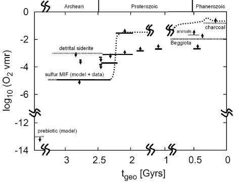
Fig. 3: A possible evolutionary path of O₂ in the atmosphere (thick dashed) which satisfies biogeochemical data. For further details: see text. Data are taken and modified from Catling and Claire (2005).

The O₂ concentration has risen from its prebiotic abundance of less than $10^{-13}$ Present Atmospheric Level (PAL) (Kasting and Donahue 1981) during the Archean eon, up to about 1% PAL by about 2.3 Gyrs ago and may have exceeded 15% PAL by about 2.1 Gyrs (e.g., Knoll and Holland 1995; Holland and Yang 2001) (see Fig. 3). Realizing the nature of the Great Oxidation Event (GOE) is central to understand the development of life on Earth and, hence, atmospheric biosignatures on Earth-like, potentially habitable extrasolar planets. Geological indices that imply an anoxic Archean atmosphere include the Mass-Independent Fractionation (MIF) of sulphur isotopes (e.g., Farquhar et al. 2000; Pavlov and Kasting 2002) and the existence of Banded Iron Formations (BIFs) (e.g., Cloud 1968; Holland 1984; Isley and Abbott 1999). On the other hand, an oxidized Archean scenario was proposed, for example, by Ohmoto (1997) based on paoleosol data. Although cyanobacteria were already present on the Earth by about 2.5 Gyrs (Summons et al. 1999), for reasons not clear the recorded rise in O₂ took place at least 200 million years later. The O₂ rise may also have changed the Earth’s climate, triggering a so-called snowball Earth (Kopp et al. 2005) possibly due to responses in the photochemistry and/or negative impacts on methanogenic bacteria leading to a decrease in the warming due to CH₄ (e.g., Zahnle et al. 2006). Note, however, that there are additional possible cooling mechanisms, for example, a change in volcanic gases (see e.g., Catling and Claire 2005). Canfield (2005) and Holland (2006) reviewed the geological evidence and current understanding of oxidative transitions in the Earth’s atmosphere. Typically, Earth system box-models (without detailed atmospheric photochemistry and climate calculations) are applied to investigate the rise in O₂. For example, Kump et al. (2001) suggested that oxidation events in the Paleoproterozoic corresponded to a mantle overturning event, where previously oxidized mantle was brought to the surface. This would lead to less-reduced gases being emitted by volcanoes and allow atmospheric O₂ to rise. Lasaga and Ohmoto (2002) applied a box model to investigate negative feedbacks of atmospheric O₂, which may account for its reasonably constant abundance since the Phanerozoic era. For example, lowering O₂, according to their results, would (1) strongly lower the weathering rate and (2) increase oceanic anoxicity and, hence, increase organic carbon burial, via less oxidation of organic carbon in the ocean column. Effects (1) and (2) are both negative feedbacks that would stabilize O₂ in the atmosphere. Holland (2003), however, questioned their model assumptions, for example, in deriving the dependence of burial rates on oxygen abundance in seawater. Catling and Claire (2005) summarized the various theories proposed to account for the rise in O₂. Briefly, these include (1) an increase in the burial rate of organic carbon and other redox-sensitive compounds, (2) an increased supply of nutrients that stimulate photosynthesis, (3) a change in volcanic gas composition or (4) a higher hydrogen escape rate from the top of the atmosphere. Claire et al. (2006) applied a zero-dimensional (0D) box-model to calculate the GOE and suggested a lowering in CH₄ as O₂ increases, whereas Goldblatt et al. (2006) suggested a bistable state (oxic and non-oxic) of the atmosphere whereby O₂ abundances would respond very strongly to small changes in surface fluxes of O₂. To explain this behavior, they proposed a positive feedback mechanism in which an initial increase in O₂ abundances leads to more O₃ and, hence, stronger UV shielding that reduces the O₂ photolytic sink and allows O₂ to build up.

1.3 Contribution of this Work

Until now, 0D box models were used to model Earth’s atmospheric O₂ evolution by evaluating the important biogeochemical processes. In these studies, the atmosphere was included in a simplified way in order to investigate CH₄ oxidation as in the works of, for example, Claire et al. (2006) and Goldblatt et al. (2006). On the contrary, there are numerical studies in which the atmospheres of early Earth and Earth-like extrasolar planets have been assessed at different time epochs by applying both one-dimensional (1D) global mean atmospheric column models as well as three-dimensional (3D) general circulation models (see e.g., Kienert et al. 2012; Charnay et al. 2013; Wolf and Toon 2013; Leconte et al. 2013; Kunze et al. 2014; Wolf and Toon 2014; Wordsworth et al. 2011).

In the case of the 1D global mean atmospheric column models investigations were performed by using either climate (see e.g., Kasting et al. 1993; von Paris et al. 2008; Goldblatt et al. 2009; Kitzmann et al. 2010; Wordsworth et al. 2010; Kitzmann et al. 2011a, b; Wordsworth and Pierrehumbert 2013) or photochemistry (see e.g., Kasting et al. 1997; Zahnle et al. 2006; Segura et al. 2007; Haqq-Misra et al. 2011) or coupled climate-photochemistry calculations (see e.g., Kasting et al. 1984; Pavlov et al. 2001, 2003; Segura et al. 2003, 2005; Grenfell et al. 2007a, b; Kaltenegger and Sasselov 2010; Rauer et al. 2011; Grenfell et al. 2011; Roberson et al. 2011; Grenfell et al. 2012) thereby neglecting biogeochemical cycles. However, since biogeochemical processes strongly influence the abundance of atmospheric constituents such as O₂ and CO₂, it is important to add these processes. Additionally, performing time-dependent integrations is a central scientific goal. However, this is currently only achievable for box-model studies (e.g., Claire et al. 2006; Goldblatt et al. 2006). Unfortunately, performing long integrations over millenia with state-of-the-art column models such as our scheme is not possible.

In this study, we have therefore developed a Coupled Atmosphere Biogeochemical (CAB) model with detailed photochemistry and climate calculations as well as biogeochemical surface processes that have an impact on atmospheric O₂. Therefore, the approach in our paper, which is similar to other atmospheric model studies (e.g., Kaltenegger and Sasselov 2010; Roberson et al. 2011), is to ”insert” Earth’s evolution, for example, via O₂ surface concentrations from proxy data and via solar luminosity changes - as a boundary condition in the CAB model. Our main motivation thereby is to focus on understanding the associated atmospheric climatological, chemical, and biological responses. Thus, we model the atmosphere and biosphere of early Earth analog planets consistently by including the effect of the fainter Sun, increased volcanic and metamorphic outgassing, and the impact of the biosphere on the atmosphere. The photochemistry atmosphere module calculates atmospheric O₂, CO₂, and molecular nitrogen (N₂) abundances self-consistently by accounting for their in situ atmospheric sources and sinks. For the early Earth analog planetary atmosphere scenarios, we apply a snap-shot-like procedure by using the Earth system as a reference. We are able to reproduce the modern Earth atmospheric composition and temperature structure. We further calculate atmospheric surface fluxes required to maintain specified O₂, CO₂, and N₂ abundances in the modern day atmosphere. For these surface fluxes we calculate with the biogeochemical module the corresponding NPP of the biospheres, which are needed to maintain the specified O₂ surface volume vmrs.

As a case study, we investigated atmospheric chemical responses of O₂ in an early Earth analog atmosphere at $10^{-6}$ PAL O₂ by applying the Pathways Analysis Program (PAP) developed by Lehmann (2004).

In the following sections, the CAB model (Section 2) and the PAP algorithm (Section 3) are decribed in detail. The CAB model is validated in Section 4. Section 5 gives an overview of the simulated early-Earth analog planet scenarios whereas in Section 6 the results are presented and discussed. Section 7 gives an overview of the sensitivity studies performed with the CAB model. We present our main conclusions in Section 8.

2 Coupled Atmosphere Biogeochemical (CAB) Model

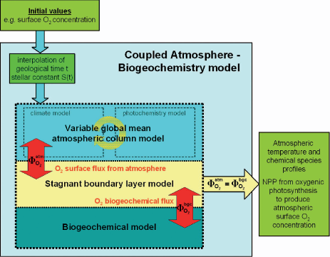
Fig. 1: Outline of the CAB model.

To study how the atmospheric, geological, chemical, and biotic systems interact, we have developed a Coupled Atmosphere Biogeochemical (CAB) model. It is composed of two submodules: 1. atmospheric climate and chemistry and 2. biogeochemistry. Both submodules are coupled via the stagnant boundary layer model (Liss and Slater 1974; Kharecha et al. 2005). The overall outline of the CAB model is given in Fig. 1. In the following sections, each submodule and their coupling will be briefly described.

2.1 Atmosphere Module Description

The ”variable” 1D global mean cloud-free, steady state atmospheric column module is based on the 1D model, which was described in detail by Kasting et al. (1984); Segura et al. (2003); Grenfell et al. (2007b, a); Rauer et al. (2011) and Grenfell et al. (2011).

The climate module calculates temperature and water profiles from the planetary surface up to the lower mesosphere by solving the radiative transfer equation. Convective adjustment is applied as a common procedure (see e.g. Manabe and Wetherald (1967); Kasting (1988); Pavlov et al. (2000); Mischna et al. (2000)) if necessary. That is, the radiative temperature gradient,$\left|\frac{dT}{dr}\right|_{rad}$, is compared to the adiabatic temperature gradient,$\left|\frac{dT}{dr}\right|_{ad}$, by calculating the convective temperature; and if the Schwarzschild criterion is fulfilled, that is, $\left|\frac{dT}{dr}\right|_{rad}>\left|\frac{dT}{dr}\right|_{ad}$, then the calculated convective temperature replaces the radiative temperature. In the troposphere a wet adiabat is calculated. The tropopause is defined as the height where both temperature profiles intersect. For the determination of the water vapor, a relative humidity distribution observed for the modern Earth from the work of Manabe and Wetherald (1967) is assumed. The radiative part of the climate module uses a longwave radiation scheme based on the work of Mlawer et al. (1997) (Rapid Radiative Transfer Model - RRTM) and a shortwave code (quadrature-$\delta$-2-stream approximation) based on the work of Toon et al. (1989). To account for the heating and cooling effects of clouds, the model’s surface albedo ($A_{\rm{surf}}$) was adjusted to 0.21 so that the converged surface temperature, $T_{\rm{surf}}$, reaches 288.15 K.

The chemistry module features more than 200 chemical reactions and calculates concentration profiles for 54 chemical species including the hydrogen- (HO_x), nitrogen- NO_x, and chlorine-oxide (ClO_x) families and sulfur-containing species, and it solves the chemical reaction network as a coupled set of continuity equations by using the backward Euler method to calculate the concentration profiles of chemical species. Below the tropopause, H₂O is given by the climate module, whereas above it is calculated self-consistently by the chemistry module according to its in situ atmospheric sources and sinks. The chemistry module accounts for wet deposition of chemical species as an atmospheric sink in the lower atmosphere by using solubility constants given by Giorgi and Chameides (1985). In the newly developed CAB model, CO₂ is also removed via rainout by introducing an effective Henry’s law constant of $3\cdot 10^{-2}$ M atm^-1 (Jacob 1999). At the model boundaries, several different boundary conditions are applied. Natural biogenic and source gas emissions of CH₄, chloromethane (CH₃Cl), CO, and nitrous oxide (N₂O) are included at the lower boundary of the model, whereas for all other species (except O₂, CO₂, and N₂, see below) dry deposition is applied. At the upper boundary an effusion flux for O and CO is used. In the CAB model, the concentrations of O₂, CO₂, and N₂ are now treated as altitude dependent,that is, similar to all other chemical species and are calculated throughout the atmosphere according to their in situ chemical sources and sinks. For all scenarios, the surface volume mixing ratio (vmr) of these chemical species is held fixed, and their corresponding atmospheric surface fluxes, $\Phi_{\rm{i}}^{\rm{atm}}$, are calculated. In this work, material surface fluxes are reported as globally averaged emission rates in g/yr. After consistent calculations of gasphase chemical vertical profiles for O₂, CO₂, and N₂ throughout the atmosphere, these profiles are transferred to the climate part where they are interpolated to the climate grid as is already done for O₃, CH₄, H₂O, and N₂O. In the new variable model version, the steady-state assumption is now applied for only two chemical species, namely atomic nitrogen (N) and excited methylene (¹CH₂), unlike previous chemistry versions of the model, which assumed steady-state for sixteen species. These two species have extremely short lifetimes, so they require the steady-state assumption in order to avoid numerical problems.

We have introduced further boundary conditions and input parameters that will be described in more detail in the following sections.

2.1.1 Volcanic and Metamorphic Outgassing

In addition to the already existing volcanic production rates from SO₂ and H₂S in the chemistry module, we have implemented volcanic outgassing rates of the chemical species H₂, CH₄, CO, and CO₂. The present-day fluxes of these chemical species are summarized in Tab. LABEL:tab1. Since the input of volcanic gases might have been higher in the past, for example, due to larger interior thermal gradients (Sleep and Windley 1982; Christensen 1985) we have introduced a heat flow parameterization, $Q(t_{\rm{geo}})$, as given by Claire et al. (2006) such that the production rate from volcanic outgassing equals

$$P_{\rm{volc,i}}=Q(t_{\rm{geo}})\cdot P_{\rm{volc,i}}^{\rm{now}}\;\;.$$ (1)

Here $P_{\rm{volc,i}}^{\rm{now}}$ is the present volcanic input flux for species i (given in Tab. LABEL:tab1). The heat flow $Q(t_{\rm{geo}})$ is a dimensionless analytical approximation depending on the geological time $t_{\rm{geo}}$ based on heat flow models that were derived from radioactive decay

$$Q(t_{\rm{geo}})=(4.5/(4.5-t_{\rm{geo}}))^{\eta}$$ (2)

where $\eta=0.7$ according to Sleep and Zahnle (2001). $t_{\rm{geo}}=0$ represents the present day.

The additional outgassing from metamorphic processes in the crust was introduced for H₂ and CH₄ based on the work of Claire et al. (2006) and taking the crustal mineral redox buffer into account. In the photochemistry module, the metamorphic production rate is implemented for H₂ as

$$P_{\rm{meta,H_{2}}}=Q(t_{\rm{geo}})\frac{\chi_{\rm{H}_{2}}P_{\rm{meta,C}}^{\rm{now}}}{1+\chi_{\rm{CH}_{4}}}$$ (3)

and for CH₄ as

$$P_{\rm{meta,CH_{4}}}=Q(t_{\rm{geo}})\frac{\chi_{\rm{CH}_{4}}P_{\rm{meta,C}}^{\rm{now}}}{1+\chi_{\rm{CH}_{4}}}$$ (4)

where $P_{\rm{meta,C}}^{\rm{now}}\sim 748$ Tg/yr is the present total flux of metamorphic CO₂ through the crust (Mörner and Etiope 2002). The parameter $\chi_{\rm{H}_{2}}$ is the metamorphic H₂/CO₂ speciation ratio and $\chi_{\rm{CH}_{4}}$ is the (CH₄+CO)/CO₂ ratio. Both values are implemented as presented in Tab. 1 in the work of Claire et al. (2006) assuming equal contributions from metamorphism of graphite saturated rocks and rocks with low graphite activity. Additionally, they depend on the oxygen fugacity, $f_{\rm{O}_{2}}$, relative to the present quartz-fayalite-magnetite (QFM) mineral redox buffer, $\Delta f_{\rm{O}_{2}}=0$, for a given crustal $p$ and $T$ conditions specified by Ohmoto and Kerrick (1977). The oxygen fugacity is usually defined as the thermodynamic activity of oxygen in equilibrium with the rock (Frost 1991). Note that for simplicity, we use the QFM buffer as our standard on going back in time although the mineral assemblage might have been more reducing in the past. Nevertheless, we have also performed sensitivity runs with a more/less reducing mineral redox buffer (see Section 7).

2.1.2 Hydrogen Escape

In the photochemical module, we have implemented the loss of H₂ due to diffusion-limited escape at the upper model boundary by introducing an effusion flux for H₂ following Walker (1977) as

$$\phi_{\rm{H}_{2}}\cong 2.5\cdot 10^{13}f_{\rm{total}}\;\;,$$ (5)

where $f_{\rm{total}}=f_{\rm{H}_{2}\rm{O}}+f_{\rm{H}_{2}}+2f_{\rm{CH}_{4}}+...$ is the sum of the vmr of all hydrogen-bearing gases above the troposphere weighted by the number of hydrogen molecules they contain. The proportionality constant, $2.5\cdot 10^{13}$, is assumed to be insensitive to differences in temperature structure and composition between a primitive and modern atmosphere. It depends on the binary diffusion parameter between the escaping species and the background atmosphere, as well as the scale height of the background atmosphere.

2.1.3 Young Sun Analog Star $\beta$ Com

The stellar input spectrum for the young sun analog G0V-dwarf star $\beta$ Com (Ribas et al. 2005) was introduced. The spectrum was derived from observations in the UV from the International Ultraviolet Explorer (IUE) satellite archive (http://archive.stsci.edu/iue), and the synthetic NextGen model spectrum at visible and near-IR wavelengths is from the work of (Hauschildt et al., 1999), who already utilized this spectrum in their general circulation model investigating the early Earth faint young sun paradox (for further details, see e.g. Kunze et al., 2014). As for Rauer et al. (2011), the spectrum was normalized to the present solar constant of 1366 W m^-2 so that the modeled planet receives the same amount of net energy at the top-of-the-atmospere (TOA) from $\beta$ Com as the Earth from the Sun. The resulting spectrum is then scaled for the different geological times following the work of Gough (1981).

2.2 Biogeochemical Module Description

The biogeochemical module applied here is based on the approach of Goldblatt et al. (2006). Therefore, we only briefly describe the main components and processes considered. Goldblatt et al. (2006) considered the atmosphere to be part of the atmosphere-ocean system and did not perform climate and photochemistry calculations. Regarding atmospheric processes, they took into account hydrogen escape and a parameterization of CH₄ oxidation. All atmospheric processes in their work are treated without a temperature dependance as atmospheric temperature is not calculated. Since CH₄ oxidation and hydrogen escape are already included in our 1D global mean atmospheric column module described in Section 2.1 they are explicitly excluded from the biogeochemical modeling described here. We furthermore split the atmosphere-ocean system used by Goldblatt et al. (2006) into the atmosphere and the ocean system. In addition to our detailed atmosphere module, described in Section 2.1, we focus on the marine environment in our biogeochemical module. This constitutes the strongest long-term source for atmospheric O₂ due to the burial of organic carbon in the ocean (continental biomass contributes only on the short-term scale and therefore, can be neglected for long-term processes).

For the biogeochemical module, we consider two reservoirs, namely, molecular oxygen ([O₂]) and buried organic carbon ([C^org]). The reservoirs are quantified in units of moles. The exchange of material fluxes between theses reservoirs are given in mol/yr and represent sources ($F_{\rm{sources}}$) or sinks ($F_{\rm{sinks}}$) for the respective reservoirs. The summation of those fluxes yields a differential equation for each reservoir according to

$$\frac{d[C_{i}]}{dt}=F_{i}^{\rm{sources}}-F_{i}^{\rm{sinks}}$$ (6)

where $[C_{i}]$ represents the considered reservoir (or chemical species).

Several biological and non-biological processes have an effect on the O₂ reservoir, and these are described in the following text. The biological processes are summarized in Tab. LABEL:biospheretab. In our model, there are two types of photosynthesis - oxygenic and anoxygenic whereby organic carbon is produced without the production of oxygen. Overall, the main context is as follows: Organic carbon produced from the different types of photosynthesis descends through the ocean column, and thereby different processes remove different fractions of the descending carbon that is finally incorporated into the ocean floor. The above is the theoretical foundation upon which the equations of Goldblatt et al. (2006) are based, and this can be described in more detail as follows: The net primary productivity (NPP) of the biosphere is described by the NPP from oxygenic photosynthesis, $N$ [mol O₂/yr], plus the additional input of inorganic reductants for anoxygenic photosynthesis, $r$ [mol O₂ equivalent/yr], which is represented by ferrous iron, Fe²⁺. Therefore, the rate of total organic carbon produced by oxygenic and anoxygenic photosynthesizers in the ocean system is $(N+r)$ (see Tab. LABEL:biospheretab). From the available organic carbon an assumed amount $\beta=0.002$ (Prentice et al. 2001; Betts and Holland 1991) is buried in sediments at the ocean floor, namely, $\beta\cdot(N+r)$ where $\beta$ is the burial efficiency. Heterotrophic aerobic respirers then use a fraction of organic carbon remaining, namely $\gamma=[\rm{O}_{2}]/(d_{\gamma}+[\rm{O}_{2}])$ (where $d_{\gamma}=3.7\cdot 10^{17}\mbox{ mol}$ corresponding to the inhibition of aerobic respiration at the Pasteur point, $\sim 0.01$ PAL (Engelhardt 1974)). Afterwards, the remaining organic carbon is used by fermenters and acetotrophic methanogens that produce CH₄ and CO₂. From the CH₄ produced, a certain fraction, namely $\delta=[\rm{O}_{2}]/(d_{\delta}+[\rm{O}_{2}])$, is oxidized by methanotrophs depending on the available O₂ concentration where $\delta_{\delta}=2.7\cdot 10^{17}\mbox{ mol, which}$ is equivalent to $[\rm{O}_{2}]=2$ $\mu$M (Ren et al. 1997). M is equivalent to mol per liter. Below the critical dissolved O₂ concentration of 2 $\mu$M, the rate of methane oxidation is inhibited.

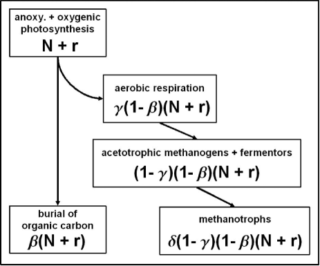
Fig. 2: Processes in the marine biosphere after Goldblatt et al. (2006). $N$ [mol O₂/yr] is the net primary productivity from oxygenic photosynthesis, $r$ [mol O₂ equivalent/yr] represents the input from anoxygenic photosynthesis. $\beta$ is the fraction of buried organic carbon. $\gamma$ resembles the fraction of aerobically respired organic carbon. $\delta$ depicts the fraction of CH₄ which is oxidized by methanotrophs.

In summary, Fig. 2 shows the total effect of the biosphere on the O₂ concentration which can be written as

$$\frac{d}{dt}[\rm{O}_{2}]^{\rm{Bio}}=\Omega([\rm{O}_{2}])N-(1-\Omega([\rm{O}_{2})])r+\beta(1-\Omega([\rm{O}_{2}]))(N+r)$$ (7)

where $\Omega([\rm{O}_{2}])=(1-\gamma)(1-\delta)=(1-\frac{[\rm{O}_{2}]}{(d_{\gamma}+[\rm{O}_{2}])})(1-\frac{[\rm{O}_{2}]}{(d_{\delta}+[\rm{O}_{2}])})$ is the fraction of the organic carbon available to decomposers. For a complete derivation of this equation, we refer the reader to the work by Goldblatt et al. (2006).

Buried organic carbon is assumed to be weathered at a rate which is determined by the rate of mechanical uplift and weathering. As in the work by Goldblatt et al. (2006), it is assumed that all organic carbon exposed by weathering is consumed by decomposers described above. The rate of weathering [C^org] is $w$[C^org]. The total effect of weathering of organic carbon for [O₂] is given according to Goldblatt et al. (2006) by

$$\frac{d}{dt}[\rm{O}_{2}]^{\rm{Cw}}=-(1-\Omega([\rm{O}_{2}]))w[\rm{C}^{\rm{org}}]\;\;.$$ (8)

For the evolution of the O₂ reservoir in the surface ocean, Eq. 7 and 8 are summed up to yield

$$\frac{d}{dt}[\rm{O}_{2}]=\Omega([\rm{O}_{2}])N-(1-\Omega([\rm{O}_{2}]))r+(1-\Omega([\rm{O}_{2}]))(\beta(N+r)-w[\rm{C}^{org}])\;\;.$$ (9)

In the same manner, we can find a differential equation for the buried organic carbon resevoir

$$\frac{d}{dt}[\rm{C}^{\rm{org}}]=\beta(N+r)-w[\rm{C}^{\rm{org}}]\;\;.$$ (10)

If we now considers steady-state conditions for the atmosphere module, then the left-hand side of Eqs. 9 and 10 are set to zero yielding a more simplified equation, namely,

$$0=\Omega([\rm{O}_{2}])N-(1-\Omega([\rm{O}_{2}]))r\;\;.$$ (11)

This equation is then solved for [O₂] using the Van Wijngaarden - Dekker - Brent root search method (Brent 1971; Press et al. 1993) (also called Brent’s method) yielding the number of moles of O₂ depending on the input from oxygenic and anoxygenic photosynthesis $N$ and $r$ (see Section 2.3). This method combines linear interpolation and inverse quadratic interpolation with bisection in order to obtain the root of Eq. 11 efficiently. To derive the aqueous O₂ concentration, we calculate according to (Goldblatt et al. 2006)

$$[\rm{O}_{2}]^{\rm{aq}}=\frac{H_{[\rm{O}_{2}]}}{\mu}[\rm{O}_{2}]$$ (12)

where $\mu=1.773\cdot 10^{20}$ mol is the number of moles in the present atmosphere (Goldblatt et al. 2006) and $H_{\rm{O}_{2}}=0.0013$ M/atm (Lide 1995) is the solubility constant of O₂ (in H₂O).

Note that since we set Eqs. 9 and 10 to zero, the burial and weathering of buried organic carbon drops out of the calculations presented. To address these processes and their impact, however, the carbon cycle also has to be implemented, which will be part of future work.

2.3 Coupling of the Atmosphere and Biogeochemical Module

The atmosphere and biogeochemistry modules are coupled via a so-called stagnant boundary layer model (Liss and Slater 1974; Kharecha et al. 2005). It calculates the biogeochemical O₂ flux, $\Phi_{\rm{O}_{2}}^{\rm{bgc}}$, defined by the different processes in Section 2.2 from

$$\Phi_{\rm{O}_{2}}^{\rm{bgc}}=\rm{v}_{p}(\rm{O}_{2})([\rm{O}_{2}]^{\rm{aq}}-H_{\rm{O}_{2}}p_{\rm{O}_{2}})C$$ (13)

where $\rm{v}_{p}(\rm{O}_{2})$ is the piston velocity of O₂, $p_{\rm{O}_{2}}$ is the atmospheric partial pressure of O₂, and $C=6.02\cdot 10^{20}$ molecules cm^-3/mol l^-1 is a units conversion factor. The piston velocity is a measure of the diffusitivity of a certain chemical species through a stagnant layer. For a chemical species i it is defined as $\rm{v}_{p}(i)=K_{\rm{diff}}(i)/z_{\rm{film}}$ with the thermal diffusivity, $K_{\rm{diff}}(i)$ and the thickness of the stagnant layer, $z_{\rm{film}}$ (here $\approx 40$ $\mu$m as in the work of Kharecha et al. (2005)). For O₂, $\rm{v}_{p}(\rm{O}_{2})$ is derived according to Wilke and Chang (1955) resulting in a value of $\rm{v}_{p}(\rm{O}_{2})\approx 5.7\cdot 10^{-3}$ cm s^-1 at 25 ^∘C.

A solution of the whole CAB model is found if

$$\Phi_{\rm{O}_{2}}^{\rm{atm}}-\Phi_{\rm{O}_{2}}^{\rm{bgc}}=0$$ (14)

where $\Phi_{\rm{O}_{2}}^{\rm{atm}}$ is calculated by the atmosphere module for a given surface vmr. Eq. 14 is also solved by applying the Van Wijngaarden - Dekker - Brent root search method. In this work, $r$ is held constant at the modern-day input of reductants into the ocean, and $N$ is varied stepwise according to the applied root search method between $N_{low}=1$ mol O₂/yr and $N_{up}=1\cdot 10^{25}$ mol O₂/yr in order to determine the input from oxygenic photosynthesis $N$ into the atmosphere that is required to maintain the prescribed atmospheric conditions.

3 Pathways Analysis Program

The Pathway Analysis Program (PAP) was developed by Lehmann (2004) to automatically identify chemical pathways in arbitrary chemical reaction networks and to quantify their efficiencies by assigning rates. PAP was applied by, for example, Grenfell et al. (2006); Verronen et al. (2011); Stock et al. (2012a, b); Grenfell et al. (2013) and Verronen and Lehmann (2013). The algorithm yields a list of all dominant pathways that produce, destroy, or recycle a chemical species of interest. PAP requires as input a complete list of chemical species and their concentrations, as well as their concentration changes caused by chemical reactions during a specified time interval. Furthermore, a complete list of reactions and their corresponding rates is required. Starting with individual reactions as initial pathways, longer pathways are formed step-by-step. For this, shorter pathways that have already been found are connected at so-called ”branching point” species, whereby each pathway that forms a branching point species is connected with each pathway that destroys it. Branching point species are chosen based on increasing lifetime with respect to the pathways constructed so far. In this work, all chemical species with a chemical lifetime shorter than that of O₂ are treated as branching point species. Since, in general, the chemical lifetime of a chemical species varies with altitude, the choice of branching point species adapts to the local chemical and physical conditions.

For the analysis of large and complex reaction networks, chemical pathways with a rate below a user-defined threshold rate $f_{\rm{min}}$ are deleted to avoid long computational time. In the present study, $f_{\rm{min}}=10^{-13}$ parts per billion by volume per second (ppbv/s)) was chosen, which is sufficient for finding all dominant pathways producing or consuming atmospheric O₂. A PAP analysis was performed for each of the 64 vertical atmospheric column module chemistry layers. The resulting production and destruction rates of O₂ from each individual pathway are integrated over the atmospheric module vertical grid and are expressed as a percentage of the total column-integrated production and destruction rate from pathways found by PAP.

4 CAB Model Validation

4.1 Atmosphere Module

The CAB model was applied to modern Earth conditions to compare the modified atmosphere module presented in this work to the previous atmosphere model version discussed byRauer et al. (2011) (denoted as RG2011), which was validated against modern Earth. Results suggest that over the calculated pressure (altitude) range a maximum relative change of the temperature profile against RG2011 between -0.5% to 0.1% is observed. The surface temperatures deviate by 0.02 K. Hence, an overall good agreement of the temperature profiles between both models was obtained.

Tab. LABEL:table:2 shows the maximum relative change in the atmosphere of relevant chemical species vmr profiles against RG2011 over altitude for O₃, H₂O, CH₄, N₂O, CH₃Cl, CO₂. For O₂ and N₂ only small deviations are obtained. Due to the introduced hydrogen escape at the upper boundary, a maximum relative change of -90% for H₂ is found (not shown) at the TOA, whereas below 40 km the change is negligible. Quite strong changes occur for sulfur-bearing species, for example, H₂S (-64%), SO₂ (-73%), SO (-72%) (not shown), because updated volcanic SO₂ and H₂S emissions were implemented, and furthermore, new volcanic emissions for H₂, CO, CH₄, and CO₂ were introduced into the CAB model (see Tab. LABEL:tab1). Despite these changes, the biosignature species, O₃ and N₂O, and biosignature related compounds, CH₄ and H₂O, compare very well with the previous global atmospheric column model used by RG2011, which is shown in Tab. LABEL:table:3.

4.2 Biogeochemical Module

For modern Earth conditions and the present input of inorganic reductants (Fe²⁺) into the ocean of $r=r_{0}=3\cdot 10^{11}$ mol Fe/yr (Holland 2006), which is equal to $r_{0}=7.5\cdot 10^{10}$ mol O₂ equivalents/yr, the CAB model calculates a global net primary productivity from oxygenic photosynthesis of $N=1.05$ Petamoles (Pmol ($10^{15}$)) O₂/yr, which is of the same magnitude as the present observed value of $N_{0}\approx 3.75$ Pmol O₂/yr (Prentice et al. 2001). The range of observed oceanic NPP varies from 2.067 - 4.167 Pmol/yr (Woodwell et al. 1978; Antoine et al. 1996; Longhurst et al. 1995), hence the lower value matches our model value within a factor of 2. The burial rate of organic carbon, $\beta(N+r)$ (see Fig. 2), calculated by the CAB model is 2.1 Tmol/yr. This value is in the range of the observed value of $10\pm 3.3$ Tmol/yr (Holland 1978). Global mean burial rates, are not well known, being based on measurements at individual sites. It is particularly challenging to estimate associated uncertainties,for example, the proxy data is severely limited in time and space and, hence, difficult to estimate in a global model.

5 Application to Early Earth Analog Atmospheres

The CAB model is applied to early Earth analog atmosphere scenarios before, during, and after the GOE at about 2.3 billion years ago. For all runs belonging to the control scenario, we assume:

• solar input spectrum (Gueymard 2004),

• surface pressure $p_{\rm{surf}}=1$ bar (as suggested by, e.g., Som et al. 2012),

• gravity acceleration $g=981$ cm s^-2,

• biogenic surface fluxes of CH₄ (474 Tg/yr), CO (1796 Tg/yr), N₂O (13.5 Tg/yr), CH₃Cl (3.4 Tg/yr) (these values are set to modern Earth conditions due to missing data), H₂ deposition velocity ($v_{\rm{dep}}=2.6\cdot 10^{-3}$ cm s^-1), and deposition velocities of other chemical compounds as in RG2011,

• crustal mineral redox buffer is set to QFM ($\Delta f_{\rm{O}_{2}}=0$),

• surface vmr of CO₂ of 355 ppm (e.g., Rosing et al. 2010, suggested only a moderate CO₂ increase of up to 3 PAL CO₂).

We use the evolutionary path of O₂ by Catling and Claire (2005) as an input parameter for the O₂ surface vmr (see Tab. LABEL:runtable), which is shown in Fig. 3 as a thick dashed line. It is constrained from upper and lower biogeochemical limits (for further details see the work of Catling and Claire 2005). Dotted horizontal lines with upper bounds (downward arrows) and lower bounds (upward arrows) show biogeochemical constraints on the O₂ partial pressure ($p_{\rm{O}_{2}}$). The existence of paleosols (Rye and Holland 1998) are indicated by unlabeled solid horizontal lines. O₂ concentrations in the prebiotic atmosphere at 4.4 Gyrs are based on numerical calculations by Kasting (1993). From the observations of MIFs in pre-2.4 Gyrs sulfur isotopes, photochemical model results of Pavlov and Kasting (2002) constrain the O₂ vmrs before 2.3 Gyrs. A lower limit for $p_{\rm{O}_{2}}$ is suggested based on the O₂ requirements of: (1) Beggiatoa emerging after 0.8 Gyrs (Canfield and Teske 1996); (2) animals appearing after 0.59 Gyrs (Runnegar 1991); and (3) charcoal production occuring after 0.35 Gyrs before present (Chaloner 1989). The high O₂ concentration around 300 Ma is based on calculations by Berner et al. (2000). We then interpolate the corresponding geological time $t_{\rm{geo}}$ given in Gyrs for a given O₂ concentration and the stellar constant $S(t_{\rm{geo}})$ is then derived from the work of Gough (1981) according to $t_{\rm{geo}}$.

The following boundary conditions are additionally varied according to the geological time $t_{\rm{geo}}$:

• volcanic emissions of H₂, H₂S, SO₂, CO, CH₄, and CO₂ and metamorphic emissions of H₂ and CH₄ (following Section 2.1.1).

6 Results

6.1 Atmosphere Modeling

6.1.1 Climate Responses

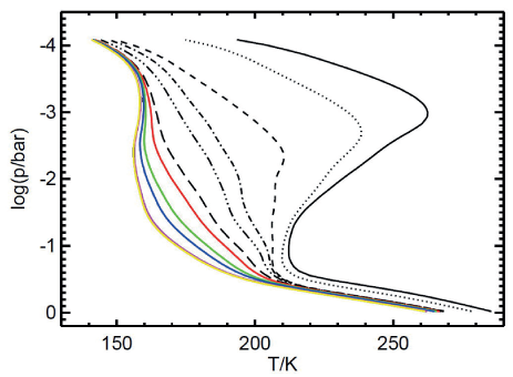
Fig. 4: Selected p-T profiles of early Earth analog atmosphere control scenario runs calculated by the CAB model. Notation: solid black: 1 PAL O₂ (modern Earth), dotted: $2.5\cdot 10^{-1}$ PAL ($t_{\rm{geo}}=0.82$ Gyrs), short dashed: $10^{-1}$ PAL ($t_{\rm{geo}}=2.18$ Gyrs), dash-dot: $2.5\cdot 10^{-2}$ PAL ($t_{\rm{geo}}=2.22$ Gyrs), dash-dot-dot-dot: $10^{-2}$ PAL ($t_{\rm{geo}}=2.22$ Gyrs), long dashed: $2.5\cdot 10^{-3}$ PAL ($t_{\rm{geo}}=2.23$ Gyrs), red: $10^{-3}$ PAL ($t_{\rm{geo}}=2.24$ Gyrs), green: $2.5\cdot 10^{-4}$ PAL ($t_{\rm{geo}}=2.25$ Gyrs), blue: $10^{-4}$ PAL ($t_{\rm{geo}}=2.28$ Gyrs), magenta: $10^{-5}$ PAL ($t_{\rm{geo}}=2.59$ Gyrs), yellow: $10^{-6}$ PAL ($t_{\rm{geo}}=2.69$ Gyrs).

Fig. 4 shows the temperature profiles of a selected number of calculated early Earth analog atmosphere runs in comparison to the modern Earth profile calculated by the CAB model. For the modern Earth p-T profile ($t_{\rm{geo}}=0$ Gyrs, solid black) the temperature decreases with decreasing pressure from $T_{\rm{surf}}=288$ K at the surface to about $T\approx 212$ K at the tropopause at $p\approx 0.1$ bar. The distinct temperature maximum at the stratopause is caused by radiative heating due to the absorption of UV radiation by O₃. At the stratopause with a pressure of $p\approx 10^{-3}$ bar a maximum temperature of $T\approx 262$ K is reached.

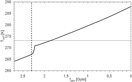
Fig. 5: Surface temperature for calculated Earth-in-time atmosphere runs. Additionally indicated as a horizontal line is the freezing temperature of H₂O of $T=273.15$ K. The beginning of the GOE at $t_{\rm{geo}}=2.3$ Gyrs is indicated as a vertical dashed line.

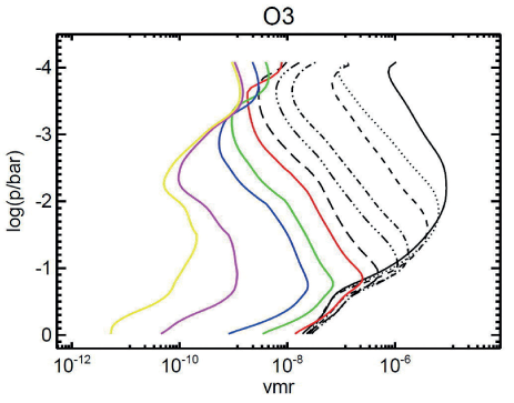
Fig. 7: O₃ profiles of Earth-in-time atmosphere runs calculated by the CAB model. Notation as in Fig. 4.

Going forwards in geological time $t_{\rm{geo}}$, the O₂ content, thereby also O₃, and the solar radiation input at the TOA increase. For the $10^{-6}$ PAL O₂ atmosphere run at $t_{\rm{geo}}=2.689$ Gyrs ago, the solar flux incident at the TOA was decreased to about 81% of the modern Earth value (”faint young Sun”). Furthermore in the low O₂ atmosphere the incoming radiation is less absorbed by molecules such as O₃ (total column: 15.8% of downwards shortwave radiation is absorbed compared to 25.5% for modern Earth) due to smaller atmospheric chemical abundances of O₃ (see Fig. 7) and other greenhouse gases. A diminishing of the temperature inversion is observed for the low O₂ atmosphere runs as a result of the low O₃ concentrations (see Fig. 7). Altogether, this leads to an increase in surface temperature (see Fig. 5) by 24 K (2.689 Gyrs ago at $10^{-6}$ PAL O₂: $T_{\rm{surf}}=264$ K, today at 1 PAL O₂: $T_{\rm{surf}}=288$ K). Note that in the case of the low O₂ atmosphere runs before 1.85 Gyrs ago, global surface temperatures are below 0^∘C implying no habitable surface conditions. Results in Fig. 4 are only applicable for modern Earth CO₂ concentrations since we have kept CO₂ at modern Earth concentrations in order to analyze the atmospheric responses on reducing surface O₂ concentrations firstly. However, see also sensitivity run G in Section 7 with 5 PAL CO₂. Further note, however, that it was recently shown by 3D general circulation models used to investigate the early Earth, for example, in the works of Wolf and Toon (2013); Kunze et al. (2014), that, even with global mean surface temperatures below the freezing point of water, areas with liquid surface ocean water could still exist, which implies habitable conditions.

Since the thermal radiation scheme RRTM is only valid for atmospheres that are quite close to modern Earth conditions (see e.g., Segura et al. 2003; von Paris et al. 2008; Rauer et al. 2011), we have compared the thermal fluxes of RRTM with thermal fluxes computed by the line-by-line radiative transfer code SQuIRRL (Schwarzschild Quadrature InfraRed Radiation Line-by-line, Schreier and Schimpf 2001; Schreier and Böttger 2003). For all runs considered the maximum relative change of net TOA fluxes calculated by RRTM vs. SQuIRRL amounted to a maximum value of -1.4 %.

6.1.2 Photochemistry Responses

UV environment

To a large extent, atmospheric chemistry is driven by the incoming TOA UV fluxes. Too understand the absorbing nature of the atmosphere, UVA (315-400 nm), UVB (280-315 nm) and UVC (176-280 nm) radiation was calculated at the surface for reduced O₂ concentration and incoming TOA solar flux. UVA and UVB wavelength ranges are taken from the International Standard (ISO 21348) 2007. Note that in the photochemistry module the term ”surface” denotes the lowermost layer at a height of about 500 m for modern Earth. In the case of the 10^-6 PAL O₂ atmosphere, the lowermost layer sinks to a height of $z_{1}=375$ m. UVA radiation at the surface stays more or less constant for atmospheres before 2.18 Gyrs. It increases from about 75 W m^-2 at $t_{\rm{geo}}=2.18$ Gyrs ago (0.1 PAL O₂) to about 90 W m^-2 for modern Earth. For the considered runs, a steady decrease from more than 12 W m^-2 to 2.3 W m^-2 is observed for surface UVB radiation before the GOE and after the GOE, respectively. The modern Earth control run exhibits a surface UVB radiation of 2.3 W m^-2, which is broadly similar to the observed value for cloud-free conditions of 1.4 W m^-2 (Wang et al. 2000). Going forward in geological time, UVC radiation decreases from 2.8 W m^-2 before 2.7 Gyrs to virtually zero $t_{\rm{geo}}=2.25$ Gyrs ago. This behavior is due to increasing O₂ and, hence, O₃ and H₂O concentrations that result in more absorption of photons in the atmosphere and more shielding of the surface from UV radiation. The impact on UVC is directly correlated with the increase in O₃, whereas UVB is affected by O₃ and H₂O together.

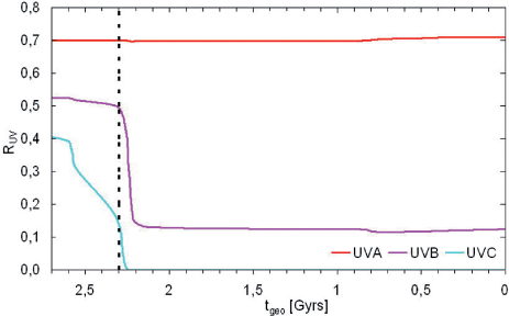
Fig. 6: Ratio (surface/TOA) radiation fluxes, $R_{\rm{UV}}$, for UVA (red), UVB (magenta) and UVC (cyan) as a function of geological time $t_{\rm{geo}}$. The beginning of the GOE at $t_{\rm{geo}}=2.3$ Gyrs is indicated as a vertical dashed line.

Fig. 6 shows the ratio surface/TOA radiation, $R_{\rm{UV}}$, as a measure of the radiation shielding efficiency of an atmosphere for UVA, UVB, and UVC radiation on going forward in geological time. For high $R_{\rm{UV}}$ values, the radiation passes efficiently through the atmosphere, whereas for $R_{\rm{UV}}=0$ it is totally blocked. UVA radiation passes efficiently through the atmosphere for all calculated runs. With the beginning of the GOE, UVB radiation is blocked rather strongly by the atmosphere, whereas UVC radiation is already starting to be blocked 2.6 Ga ago. After the GOE the atmosphere is totally opaque for UVC radiation. Possible negative impacts on organisms in the marine environment before the GOE might have been reduced due to the Urey effect (Urey 1959) where a small quantity of O₂ produced during photosynthesis of H₂O absorbs a considerable amount of UV radiation. For modern Earth, UVB radiation is almost totally blocked by the atmosphere.

In the following photochemical analysis, we only focus on the impact on important atmospheric constituents such as biosignatures (O₃, N₂O, O₂) and related bioindicators (CH₄, H₂O) as well as CO₂. ”Bioindicators” are indicative of biological processes but can also be produced abiotically.

Ozone - O₃

O₃ is suggested to be a biosignature because it is formed in the stratosphere mainly from molecular oxygen via the Chapman mechanism (Chapman 1930), which is initiated by the photolysis of mostly biogenic O₂. In the troposphere O₃ is produced via the smog mechanism (Haagen-Smit 1952), which requires O₂, volatile organic compounds, nitrogen oxides, and UV radiation. The destruction of O₃ in the stratosphere proceeds via catalytic cycles that involve, for example, HO_x, NO_x, or ClO_x (e.g., Bates and Nicolet 1950; Crutzen 1970), which are stored in reservoir species and can be activated by changes in, for example, temperature or UV radiation. In the troposphere, O₃ is removed via wet/ dry deposition, photolysis, or reactions with NO_x, HO_x and unsaturated hydrocarbons.

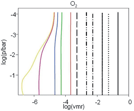
Fig. 16: O₂ profiles of Earth-in-time atmosphere runs calculated by the CAB model. Notation as in Fig. 4.

Fig. 7 shows the O₃ vmr profiles for reduced O₂ content of the atmosphere. Modern Earth’s O₃ layer (solid black) exhibits a distinct maximum at about 0.01 bar due to the mechanisms decribed above. Fig. 7 suggests that, for reduced O₂ concentrations, the O₃ layer moves to higher pressures (lower altitudes), for example, for 10^-5 PAL to 0.2 bar, because in consequence of a lower O₂ concentration, less O₃ is produced at the same altitude. This results in increased UV radiation in atmospheric layers directly below, which stimulates the Chapman mechanism and produces more O₃, and hence the peak of the O₃ layer moves to lower altitudes. However, if O₂ concentrations fall below those of CO₂ ($=3.6\cdot 10^{-4}$, left of the green line), results are consistent with CO₂ photolysis now being the major source for atomic oxygen (O) and, hence, O₃. The O₃ peak moves upwards where CO₂ is photolyzed more easily. Additionally, in the upper atmosphere a second O₃ maximum becomes visible, which is related to an increase in O₂ vmr toward lower pressures (see Fig. 16). Note that for modern Earth this secondary O₃ maximum lies in the vicinity of the mesopause (see e.g., Evans et al. 1968; Hays and Roble 1973; Smith and Marsh 2005) and arises due to the interplay between active-hydrogen and active-oxygen chemistry, relatively low temperatures, and a local maximum of O (Allen et al. 1984; Smith and Marsh 2005).

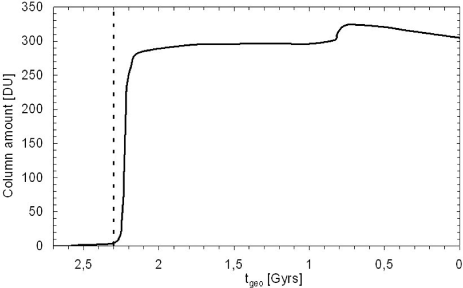
Fig. 8: O₃ column [DU] amount as a function of geological time $t_{\rm{geo}}$ for considered Earth-in-time atmosphere runs. The beginning of the GOE at $t_{\rm{geo}}=2.3$ Gyrs is indicated as a vertical dashed line.

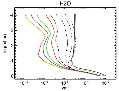
Fig. 9: H₂O profiles of Earth-in-time atmosphere runs calculated by the CAB model. Notation as in Fig. 4.

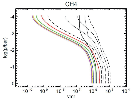
Fig. 13: CH₄ profiles of Earth-in-time atmosphere runs calculated by the CAB model. Notation as in Fig. 4.

The change in overall O₃ column amount on going forwards in geological time is shown in Fig. 8. It increases from zero before the GOE to 296 DU after the GOE. At about 0.8 Gyrs ago, a Second Oxidation Event (SOE) occured resulting in an increase of the O₃ column amount to 325 DU. Afterward, it decreases to the modern Earth value of 305 DU. To illustrate this decrease in O₃, we have included Fig. 9, in which it can be seen that the troposphere becomes damper (going forward in time) due to evaporation because of increasing surface temperatures. However, in the stratosphere this is not always the case (compare the solid black line with the short-dashed and dotted line). A dryer stratosphere leads to less HO_x and, hence, enhanced NO_x resulting in an increase in catalytic O₃ loss. The dryer stratosphere is a result of a decrease in CH₄ (see Fig. 13) that is driven by OH, which has a complex photochemistry. Berkner and Marshall (1965) estimated that effective UV shielding would be provided by a column amount of 200 DU, which is reached in this work at $t_{\rm{geo}}=2.22$ Gyrs ago (0.025 PAL O₂), whereas Ratner and Walker (1972) adopted a more stringent lower limit on the O₃ column amount of 259 DU (reached in this work at $t_{\rm{geo}}=2.19$ Gyrs ago (0.1 PAL O₂)).

Water - H₂O

In the case of modern Earth, the water vapor vmr in the troposphere is chemically inert and subject to the hydrological cycle. Above the tropopause, however, the H₂O vapor concentration is determined by its chemical sources (here, CH₄ oxidation) and sinks as well as transport from the troposphere and approaches an isoprofile for the modern Earth.

Fig. 9 shows the H₂O vapor vmr profiles on decreasing ground level O₂ concentrations on going back in time. The solar flux incident at the TOA decreases, which results in a decrease in surface temperature and, hence, condensation of H₂O in the troposphere. The atmosphere becomes dryer due to decreasing surface temperatures. The stratospheric H₂O profile deviates from the isoprofile (found for modern Earth), and a distinct maximum develops in the early Earth analog runs. In this region, H₂O is primarily produced from O₂ (which increases in this region - see later) via the net reaction CH₄ + O₂ $\rightarrow$ H₂O + H₂ + CO which is initiated by the photolysis of CH₄. Furthermore, H₂O is predominantly destroyed via photolysis in the low O₂ atmosphere due to enhanced UV radiation resulting in the formation of H₂ and CO₂.

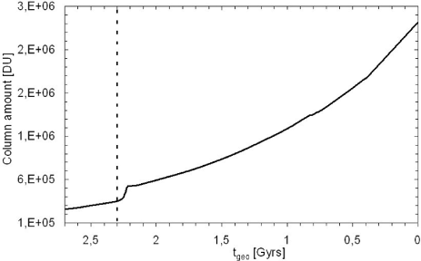
Fig. 10: H₂O column amount [DU] as a function of geological time $t_{\rm{geo}}$ for Earth-in-time atmosphere runs considered. The beginning of the GOE at $t_{\rm{geo}}=2.3$ Gyrs is indicated as a vertical dashed line.

The overall H₂O column amount increases on going forwards in geological time as shown in Fig. 10 which can be attributed directly to the temperature behavior shown in Fig. 5. There is a caveat, however, that there could be deviations in our temperature behavior in comparison to the geological record.

Nitrous oxide - N₂O

N₂O is an important biosignature. For modern Earth, it is almost exclusively produced by bacteria as part of the (de)nitrifying cycle (IPCC 2001). It is destroyed mainly in the stratosphere via photolysis or via the reaction with excited oxygen (O(¹D)).

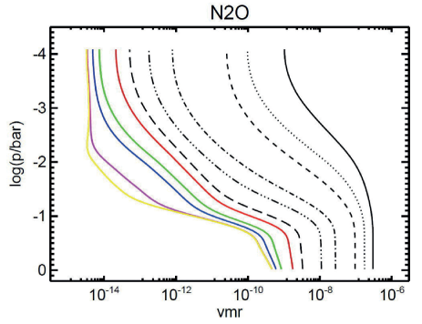
Fig. 11: N₂O profiles of Earth-in-time atmosphere runs calculated by the CAB model. Notation as in Fig. 4.

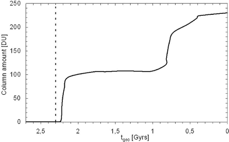
Fig. 12: N₂O column amount [DU] as a function of geological time $t_{\rm{geo}}$ for Earth-in-time atmosphere runs considered. The beginning of the GOE at $t_{\rm{geo}}=2.3$ Gyrs is indicated as a vertical dashed line.

Fig. 11 shows the N₂O vmr profiles for decreased ground level O₂ concentrations. N₂O destruction via photolysis becomes more efficient in the atmosphere due to increased UV radiation for atmospheres with lower O₂ surface vmrs. This results in decreased N₂O concentrations and, hence, lower column amounts (shown in Fig. 12) in the geological past. In situ inorganic production of N₂O is negligibly small.

Methane - CH₄

Atmospheric CH₄ is a bioindicator since in addition to biogenic sources some geological sources exist. CH₄ is destroyed in the atmosphere mainly by the reaction with hydroxyl (OH) and in the upper stratosphere by photolysis.

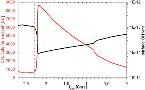
Fig. 14: CH₄ column amount [DU] (red) and surface OH vmr (black) as a function of geological time $t_{\rm{geo}}$ for Earth-in-time atmosphere runs considered. The beginning of the GOE at $t_{\rm{geo}}=2.3$ Gyrs is indicated as a vertical dashed line.

Fig. 13 shows the CH₄ profiles for reduced ground level O₂ concentration. Note, however, that we fixed the biological surface flux for all scenarios considered. But see also sensitivity run H in Section 7, which considers a doubled flux. For increasing O₂ concentrations, CH₄ increases as well, reaches a maximum at 0.1 PAL O₂, and then decreases toward higher O₂ values. The corresponding column amounts are given in Fig. 14. The maximum in CH₄ column amount at $t_{\rm{geo}}=2.18$ Gyrs (0.1 PAL O₂ vmr) is directly linked with a minimum concentration of OH and, hence, minimum destruction of CH₄, at the same geological time. For modern Earth, standard OH sources are, for example, H₂O + O(¹D) $\rightarrow$ OH + OH (where O(¹D) arises mainly from O₃ photolysis) and sinks, for example, CO + OH $\rightarrow$ CO₂ + H and OH + HO₂ $\rightarrow$ H₂O + O₂. Note that the first sink reaction allegedly destroys OH. Most of the H atoms formed react quickely via the reaction H + O₂ + M $\rightarrow$ HO₂ + M followed by, for example, HO₂ + O₃ $\rightarrow$ OH + 2O₂, which reforms OH, and thus the reaction between CO and OH does not lead to an efficient OH loss. The second loss reaction is a more permanent sink for OH. The main source of OH switches to H₂O + h$\nu$ $\rightarrow$ H + OH for the low O₂ atmospheric run due to higher UV.

Fig. 14 illustrates an important result of our work, that is, we calculate an increase in CH₄ concentration with increasing O₂ vmrs at the GOE. Previous works (e.g., Claire et al. 2006; Zahnle et al. 2006) with much simpler chemical schemes, however, suggest the opposite effect, namely, that increasing O₂ (more oxidizing conditions) would lead to stronger CH₄ oxidation (into CO₂ and H₂O) and, hence, a reduction in CH₄. This behavior is hypothesized by the authors to lead to a Snowball Earth. CH₄-oxidation is a complex multireaction process that usually begins by attacking OH on CH₄. OH is photolytically produced, which (generally) means high OH abundances in high UV atmospheres, all else being equal. In our study, an increase in O₂ leads to an increase in O₃, which blocks UV. This leads to less OH and, hence, more CH₄. Our work suggests that more investigations are required in the chemical feedbacks between CH₄ and O₂ on the early Earth. After the GOE, O₂ further increases and CH₄ is more and more destroyed via the reaction with OH, which then increases because of higher production via, for example, H₂O + O(¹D) $\rightarrow$ 2OH (since H₂O increases as discussed). Note that in our study we assume a constant biogenic input of CH₄ of 474 Tg/yr at the surface for every run considered. This value could be rather weak for the early Earth (see Claire et al. 2006). Also, due to the toxic nature of O₂ to CH₄ producing microorganisms, the rise in O₂ likely had a severe impact on the biological activity and produced atmospheric CH₄, therefore, resulting in a dramatic decrease in biotic CH₄ production. This mechanism is not included in the CAB model, and is beyond the scope of this paper.

Carbon dioxide - CO₂

CO₂ is an important greenhouse gas that is generally well mixed in the modern Earth atmosphere.

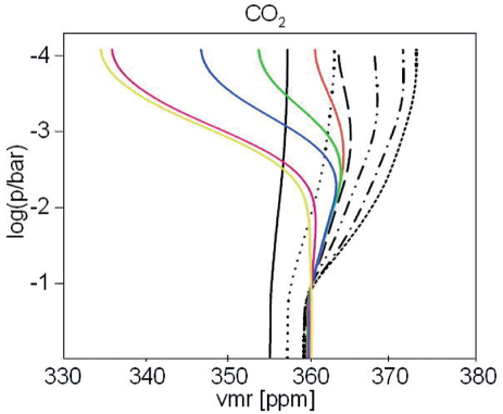
Fig. 15: CO₂ profiles of Earth-in-time atmosphere runs calculated by the CAB model. Notation as in Fig. 4.

Fig. 15 shows how the CO₂ vmr profiles change on decreasing the ground level O₂ concentrations. For decreases down to 0.1 PAL O₂, CO₂ increases in the stratosphere mainly due to the HO_x catalyzed net reaction O₃ + 3CO $\rightarrow$ 3CO₂, which is initialized by the catalyzed photolysis of O₃ and O₂. For further decreases in O₂, stronger photolysis of CO₂ leads to decreased vmrs in the stratosphere. This implies that CO₂ does not exhibit an isoprofile throughout the atmosphere for low O₂ concentrations. In the case of 10^-6 PAL O₂, the TOA vmr of CO₂ is 334 ppm in comparison to the surface vmr of 355 ppm. There is a caveat, however: CO₂ profiles could depend on the rather unconstrained value of the eddy diffusion profile $K(z)$.

Molecular oxygen - O₂

Fig. 16 shows that O₂ exhibits an isoprofile behavior for atmosphere runs with ground level O₂ concentrations above $10^{-4}$ PAL O₂, which implies that its concentration is dominated by transport processes rather than chemical production ($P$) and destruction ($L$). For the atmosphere runs with surface O₂ concentrations below $10^{-4}$ PAL O₂, an anti-correlation between the vertical CO₂ and O₂ profiles becomes visible implying that the destruction of CO₂ provides a source of atmospheric O₂ in the upper stratosphere. A detailed chemical analysis will be presented in Section 6.1.3 to gain detailed insight into the rather complex production (and destruction) processes for O₂.

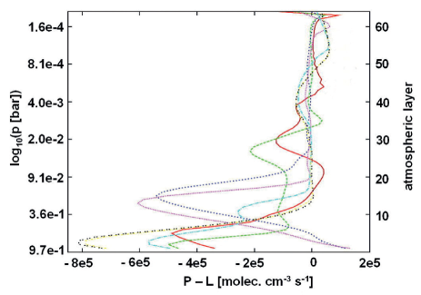
Fig. 17: Atmospheric net $(P-L)$ chemical change of O₂ calculated by the CAB model for modern Earth and low O₂ atmospheres. Notation: solid red: 1 PAL O₂ (modern Earth), dashed green: $10^{-1}$ PAL ($t_{\rm{geo}}=2.18$ Gyrs), dotted dark blue: $10^{-2}$ PAL ($t_{\rm{geo}}=2.22$ Gyrs), dotted purple: $10^{-3}$ PAL ($t_{\rm{geo}}=2.24$ Gyrs), dot-dashed cyan: $10^{-4}$ PAL ($t_{\rm{geo}}=2.28$ Gyrs), dot-dashed yellow: $10^{-5}$ PAL ($t_{\rm{geo}}=2.59$ Gyrs), dot-dot black: $10^{-6}$ PAL ($t_{\rm{geo}}=2.69$ Gyrs).

Fig. 17 compares the net chemical change

$$(\Delta n_{i})_{\rm{chem}}=P_{i}-L_{i}$$ (15)

of $i=\rm{O}_{2}$ in the atmosphere for modern Earth and low O₂ atmospheres. Thereby, $n_{i}$ is the number density of the chemical compound $i$. For modern Earth O₂ is only produced immediately below and above the O₃ layer maximum in the stratosphere. In general, O₂ is mostly destroyed in the atmosphere except for the lowermost atmospheric layers of atmospheres with ground level concentrations between 10^-2 and 10^-3 PAL. For very low O₂ atmospheres there is a net production at the uppermost layers which is a result of increased CO₂ photolysis as mentioned above.

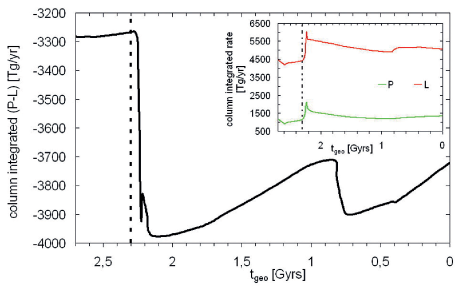
Fig. 18: Column integrated net $(P-L)$ chemical change of atmospheric O₂ calculated by the CAB model as a function of geological time $t_{\rm{geo}}$ for Earth-in-time atmosphere runs considered. The beginning of the GOE at $t_{\rm{geo}}=2.3$ Gyrs is indicated as a vertical dashed line. In the upper right panel the column-integrated P (green) and L (red) rates are given as a function of geological time $t_{\rm{geo}}$ for comparison.

Fig. 18 depicts the net column integrated (global mean) $(P-L)$ chemical change of O₂ calculated by the CAB model on going forward in geological time. Addidionally, in the upper right of Fig. 18 the column-integrated production and destruction rates of O₂ are shown for comparison. This illustrates that O₂ is generally destroyed within the atmosphere for all runs considered. Hence, this indicates that a positive O₂ flux of the same amount into the atmosphere is required in order to achieve steady-state and maintain O₂ levels above zero. It is striking that although the surface O₂ concentration varies by several orders of magnitude, the associated O₂ surface flux, $\Phi^{\rm{atm}}_{\rm{O}_{2}}$, into the atmosphere varies between about 3300 and 4000 Tg/yr by only about 20%. Before the GOE it exhibits an almost constant behavior. In this atmosphere regime, small changes in the O₂ surface flux can support a wide range of different surface O₂ vmrs (not shown). Then, $\Phi^{\rm{atm}}_{\rm{O}_{2}}$ increases sharply during the GOE as surface O₂ concentrations increase strongly. After the GOE, $\Phi^{\rm{atm}}_{\rm{O}_{2}}$ decreases, followed by a sharp increases at the SOE at 0.8 Gyrs ago and then decreases again. Generally, one recognizes that the mathematical solution is not unique, that is, for one atmospheric O₂ surface flux there are multiple surface O₂ vmrs regarding the different boundary conditions. This means that the same magnitude of O₂ surface flux (which is a measure of the strength of the chemical production and destruction of O₂ in the whole atmosphere) can support either (a) an anoxic atmosphere or (b) a rather oxic atmosphere (which in turn depends on other established factors known to affect O₂(g) such as irradiation and volcanic/ metamorphic outgassing). The biosphere productivity that corresponds to the O₂ surface flux at different ground level O₂ concentrations is investigated in Section 6.2.

Comparison to previous work

Generally, it is not easy to compare results with those of previous works in the literature regarding the early Earth since either, for example, only stand-alone photochemical models (i.e., without coupled climate calculations) have been presented (e.g. Kasting and Donahue 1980; Kasting 1982; Kasting et al. 1985; Zahnle et al. 2006) or coupled climate-chemistry calculations performed using an isoprofile assumption for O₂, CO₂ and N₂ (e.g. Segura et al. 2003). Furthermore, previous workers have assumed increased CO₂ vmrs (see e.g., Kasting et al. 1984) and CH₄ surface fluxes (see e.g., Pavlov et al. 2003) to be present in the early Earth atmosphere.

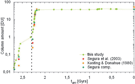
Fig. 19: Column amount of atmospheric O₃ in DU as a function of geological time $t_{\rm{geo}}$ for Earth-in-time atmosphere runs considered in comparison to previous work. The beginning of the GOE at $t_{\rm{geo}}=2.3$ Gyrs is indicated as a vertical dashed line.

Some key chemical reactions resulting in the production and destruction of O₂ have, however, also been identified, for example, in Kasting et al. (1984) although calculated O₂ profiles differ from this work. Focusing on atmospheric O₃, Fig. 19 shows a comparison of the O₃ column depth calculated by this study with those of Segura et al. (2003) and Kasting and Donahue (1980). To compare with the work of Segura et al. (2003), additional runs were performed with the CAB model (”Segura comp.” shown in dark green) with the initial atmospheric conditions as in the Segura et al. (2003) study. A further important result of this work is shown in Fig. 19, where it can be seen that, due to our atmosphere model improvements, we calculate a consistently enhanced O₃ column amount compared to previous works in the literature. This difference calculated in O₃ occurs, for example, due to an increased photolytic destruction of CO₂ in the runs of this work leading to production of O₂ and, hence, O₃. Comparing results of the Segura comp. runs with the results of Segura et al. (2003) suggests, for example, a maximum relative change in the O₃ column amount of 82% at $t_{\rm{geo}}=2.28$ Gyrs ($10^{-4}$ PAL O₂). For H₂O, N₂O and CH₄ qualitatively similar results were found.

6.1.3 Pathway Analysis with respect to O₂

For the early Earth analog runs, model calculations generally predict an increase of the O₂ vmr with increasing atmospheric height, which implies an in situ atmospheric source of O₂ (see Fig. 16). Furthermore, it can be seen that the CO₂ profile is anti-correlated with the O₂ profile in the low O₂ Earth-in-time atmosphere runs (see Fig. 15). This might imply that CO₂ serves as a source species for O₂. Our goal is to identify how O₂ is produced from CO₂ in the presence of highly reactive radicals such as OH. We further focus on the O₂ destruction pathways to identify the dominant reduced chemical species that are responsible for the consumption of O₂. Therefore, the Pathway Analysis Program (PAP) (for details see Section 3) is applied for an atmosphere with a surface O₂ vmr of $10^{-6}$ PAL O₂ ($t_{\rm{geo}}=2.688$ Gyrs). Our study represents the first application of PAP in the context of the early Earth. We consider only pathways with an individual contribution larger than 1.5% of the total production (or destruction) of O₂.

In the analysis, we firstly considered all chemical species with an in situ chemical lifetime smaller than that of O₂ as a branching point as described in Section 3. It turned out that CO is part of the net reactions of the dominant O₂ production and destruction pathways, respectively. This indicates, that for the rates of O₂ production and destruction pathways, it is relevant whether CO is treated as a branching point or not (if it is, all CO production and destruction pathways will be combined as far as possible to yield null cycles, i.e., pathways which do not have a net effect on CO; if it is not, CO production and destruction pathways are not combined). For about 40% of the atmospheric layers considered, CO was used as a branching point. To ensure a consistent treatment of all O₂ production and destruction pathways at every atmospheric height, we repeated the analysis by excluding CO as a branching point.

Production pathways and their altitude dependence

Tab. LABEL:proPAPpathstab summarizes the major column-integrated chemical production pathways, P1 - P7, found by PAP and their percentage contributions to the total column-integrated O₂ production rate for an atmosphere with a surface O₂ vmr of $10^{-6}$ PAL O₂.

The major column-integrated chemical production pathways presented in Tab. LABEL:proPAPpathstab can be categorized into 2 classes as follows:

• class PA:
  O₂ is produced by pathways with the net reaction
  2CO₂ $\rightarrow$ O₂ + 2CO

  • subclass PA1 (P1, P2, P7): catalyzed by HO_x species,

  • subclass PA2 (P3, P4): without the presence of HO_x,

• class PB:
  O₂ is formed by pathways with the net reaction 2O $\rightarrow$ O₂

  • subclass PB1 (P6): catalyzed by HO_x species,

  • subclass PB2 (P5): without the presence of HO_x.

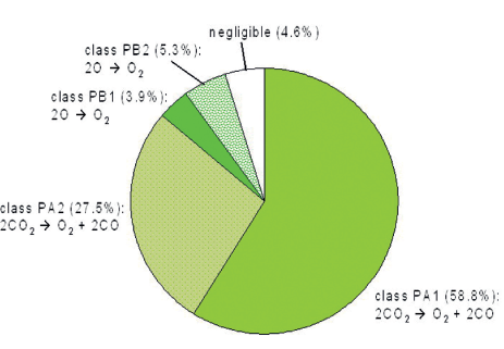
Fig. 20: O₂ production classes (see Tab. LABEL:proPAPpathstab) and their contributions to the total column-integrated O₂ production rate via pathways calculated by PAP for an Earth-like atmosphere with a surface O₂ vmr of $10^{-6}$ PAL O₂.

The relative contributions of the pathways mentioned above to the total column-integrated production rate are given in Fig. 20. Pathways of subclass PA1 and PA2 are initiated by the photolysis of CO₂, whereas class PB pathways require overall the presence of atomic oxygen. The main source for O originates from the photolysis of CO₂ in the upper stratosphere producing O(¹D) and, hence, O, which is then transported downwards by eddy diffusion, contributing to enhanced O₂ vmrs in the upper stratosphere. Note that at the upper boundary of the photochemistry part of the atmosphere module an effusion flux for O and CO is implemented to simulate this effect from atmospheric layers above the module TOA. Pathway P2 was found by Yung and DeMore (1999) in the context of a pure CO₂ dominated atmosphere.

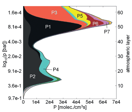
Fig. 21: Altitude dependence of O₂ production pathways P1 to P7 (see Tab. LABEL:proPAPpathstab) for an Earth-like atmosphere with a ground level O₂ concentration of 10^-6 PAL.

Fig. 21 shows the altitude dependence of the production pathways of O₂ for an Earth-like atmosphere with a surface O₂ vmr of $10^{-6}$ PAL O₂, which indicates that the production of O₂ in the atmosphere is strongest in the upper stratosphere. The total production rate due to chemical pathways calculated by PAP is also shown (solid black line). About 98.7% of the total column-integrated O₂ production rate are explicable via pathways found by PAP with individual contributions above 1.5%. The dominant production pathways P1 and P3 (as well as P7), which produce excited oxygen (O(¹D)) from CO₂ photolysis, act in the upper stratosphere where UV radiation is strongest. As the UV radiation passes through the atmosphere, it is absorbed and, hence, the second dominant pathway P2 (and also P4), which involves ground-state oxygen (O) instead of O(¹D), has its maximum rate at lower altitudes. Due to the enhanced O abundance in the upper stratosphere, which is provided from CO₂ photolysis that produces O(¹D) and is transported downward to the analyzed atmospheric layers, the pathways P5 and P6 have their maximum rate in the upper stratosphere. Note that, except for the photolysis of CO₂, pathways P5 and P6 are equal to P4 and P2.

Destruction pathways and their altitude dependence

Tab. LABEL:lossPAPpathstab summarizes the major column-integrated chemical destruction pathways and their percentage contributions to the total column-integrated O₂ destruction rate found by PAP for an atmosphere with a surface O₂ vmr of $10^{-6}$ PAL O₂.

These pathways can be categorized into 4 classes:

• class LA:
  O₂ is destroyed by pathways with the net reaction O₂ + 2CO $\rightarrow$ 2CO₂ (CO-oxidation) which are catalyzed by HO_x and NO_x species

  • subclass LA1 (L1, L2, L6, L8): initialized by the oxidation of H,

  • subclass LA2 (L3, L5): initiated by the photolysis of O₂,

• class LB:
  O₂ is consumed by CH₄-oxidation pathways

  • subclass LB1 (L4, L7): net reaction 3O₂ + 2CH₄ $\rightarrow$ 4H₂O + 2CO,

  • subclass LB2 (L10): net reaction O₂ + CH₄ $\rightarrow$ H₂O + H₂ + CO,

• class LC (L9):
  O₂ is consumed by pathways with the net reaction O₂ + 2H₂ $\rightarrow$ 2H₂O (H₂-oxidation),

• class LD (L11):
  O₂ is consumed by pathways with the net reaction O₂ + H₂O + CO $\rightarrow$ H₂O₂ + CO₂.

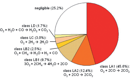
Fig. 22: As for Fig. 20 but for destruction (see also Tab. LABEL:lossPAPpathstab).

Their relative contributions to the total destruction rate via pathways are given in Fig. 22. Generally, O₂ is consumed forming CO₂, CO, H₂, H₂O, and H₂O₂. Pathways of class LA lead to the oxidation of CO mainly via HO_x. Thereby, in the subclass LA2 pathways are initiated by the photolysis of O₂. The complex pathways of the subclasses LB1 and LB2 destroy O₂ via the oxidation of CH₄, whereas class LC leads to the oxidation of H₂. Furthermore, there is a small contribution from class LD that leads to the formation of H₂O₂ via oxidation of CO and H₂O. This is rather surprising since H₂O₂ is a highly reactive (oxidizing) tropospheric species (produced by self-reaction of HO₂ and removed via photolysis and fast surface deposition). H₂O₂ features a lifetime of typically a few hours and is therefore set to be a branching point species throughout the troposphere (see Section 3). Nevertheless, L11 suggests a pathway in which H₂O₂ is overall produced. We interpret this result as follows: PAP was supplied with input from rate data for chemical reactions that occur only (in situ) in the atmosphere. It was not supplied with rates for other processes such as dry and wet deposition. Since H₂O₂ features a rapid depositional surface sink, and therefore to attain an equilibrium concentration for this species in the atmospheric model, there must exist a pathway in the atmosphere that overall forms a net source of H₂O₂, to balance the strong surface depositional sink. It is this net source that PAP has found in the form of L11.

Several pathways shown in Tab. LABEL:lossPAPpathstab have also been found by previous workers in the context of the martian atmospheric chemistry, for example, L1 by Parkinson and Hunten (1973) and Yung and DeMore (1999), L2 by Stock et al. (2012a), L3 by McElroy and Donahue (1972), L6 by Nair et al. (1994) and Yung and DeMore (1999), and L8 by Sonnemann et al. (2006). This implies that pathways that are important for the CO₂-dominated martian atmosphere may also play a key role in an Earth-like atmosphere with low O₂ and 1 PAL CO₂ abundances.

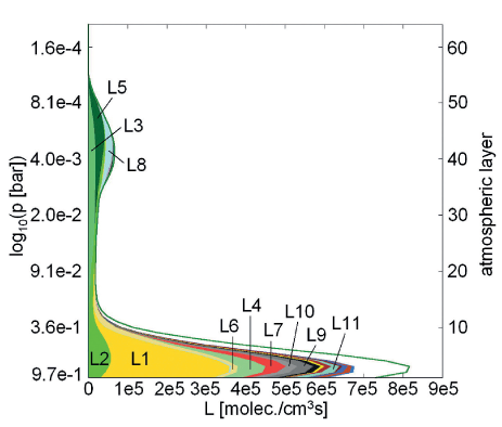
Fig. 23: As for Fig. 21 but for destruction (see also Tab. LABEL:lossPAPpathstab).

Fig. 23 shows the altitude dependence of the O₂-consumption pathways for an Earth-like atmosphere with a surface O₂ vmr of $10^{-6}$ PAL O₂. The total destruction rate due to chemical pathways calculated by PAP is also shown (solid green line). About 84.1% of the total column-integrated O₂ destruction rate is due to pathways with individual contributions above 1.5%. Especially, in the troposphere the destruction of O₂ is composed of a large number of pathways, which individually contribute less than 1.5% to the total column-integrated destruction rate. Fig. 23 suggests two regimes for the destruction of O₂ in the atmosphere as follows:

• The main consumption of O₂ in the troposphere occurs via the oxidation of reduced gases such as CO, CH₄, and H₂ (but only to a very small amount ($<1.5$%) by reduced sulfur such as H₂S) and is composed of a large number of different pathways. The dominant pathway L1 leads to CO-oxidation catalyzed by HO_x (CO is provided by diffusion from the upper atmosphere where it is strongly produced from CO₂ photolysis), whereas the complex CH₄ oxidation pathways L4, L7, and L10 have smaller contributions. Note that our results may change depending of the CH₄ concentration and, hence, biological CH₄ flux inserted at the surface. The minor pathway L9 results in the oxidation of H₂, which is delivered by volcanic emissions from the surface and via diffusion from the upper atmosphere. H₂ is destroyed in situ in the lower atmosphere. There is an additional small contribution from pathway 11 that results in the oxidation of CO in the presence of H₂O.

• A minor contribution (L3, L5, and L8) to the destruction pathways originates in the stratosphere. At these altitudes O₂ consumption during CO oxidation is most efficient due to a maximum in HO₂ abundance (not shown), whereby pathways L3 and L5 are initiated by the photolysis of O₂.

In summary, for an Earth-like atmosphere with low surface O₂ concentrations ($10^{-6}$ PAL O₂) atmospheric O₂ is produced in the upper stratosphere mainly from the in situ photolytic destruction of CO₂ (whereas a small contribution relies on the delivery of O by atmospheric diffusion). O₂ is mainly destroyed in the lower atmosphere by complex pathways resulting mainly in the formation of H₂O and CO₂ via the oxidation of CO, CH₄, and H₂. Thereby, there is a minor contribution from pathways resulting in the formation of H₂ and H₂O₂. In both the production and destruction of O₂, CO plays a key role. Note that the abiotic in situ production rate of O₂ in the atmosphere from CO₂ photolysis as well as the O₂ destruction rate are comparatively smaller than the O₂ flux originating from the surface biosphere.

6.2 Biogeochemical Modeling

The CAB model calculates how much input from oxygenic photosynthesis, $N$ (NPP), is needed to maintain the surface flux $\Phi^{atm}_{\rm{O}_{2}}$ calculated by the atmospheric chemistry module for a given surface vmr of O₂.

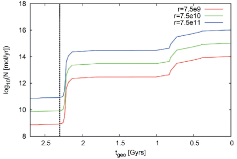
Fig. 24: Calculated input from oxygenic photosynthesis, $N$, in mol O₂ per year for a constant value of anoxygenic photosynthesis, $r$, as a function of geological time $t_{\rm{geo}}$: $r=7.5\cdot 10^{10}$ mol O₂ equiv./yr is the present value (Holland 2006) (green), $r=7.5\cdot 10^{11}$ mol O₂ equiv./yr is an upper limit for the Archean (Holland 2006) (blue) and for comparison calculations were performed for a constant value of $r=7.5\cdot 10^{9}$ mol O₂ equiv./yr (red). The beginning of the GOE at $t_{\rm{geo}}=2.3$ Gyrs is indicated as a vertical dashed line.

Assuming three constant inputs from anoxygenic photosynthesis ($r=7.5\cdot 10^{9}$, $7.5\cdot 10^{10}$ (present value, Holland 2006), and $7.5\cdot 10^{11}$ mol O₂ equiv./yr (Archean upper limit, Holland 2006)), Fig. 24 shows the resulting $N$ as a function of geological time $t_{\rm{geo}}$.

Before the GOE at about 2.3 Gyrs $N$ exhibits an almost constant behavior, although O₂ concentrations vary over two orders of magnitude (see Tab. LABEL:runtable). After the GOE, it increases modestly with increasing O₂ concentrations and does not reflect the sometimes oscillating behavior found for the atmospheric O₂ surface flux (see $(P-L)$ chemical change behavior in Section 6.1.2 for comparison). On inserting Eq. 13 into Eq. 14 one obtains

$$\Phi_{\rm{O}_{2}}^{\rm{atm}}=\rm{v}_{p}(\rm{O}_{2})([\rm{O}_{2}]^{\rm{aq}}-H_{\rm{O}_{2}}p_{\rm{O}_{2}})C\;\;.$$ (16)

Eq. 16 can now be rearranged for $[\rm{O}_{2}]^{\rm{aq}}$, which is calculated by the biogeochemical module (see Eq. 11 and 12) and directly depends on $N$. For $N$, two regimes can then be identified as follows:

• Regime I (low O₂ regime before the GOE): $H_{\rm{O}_{2}}p_{\rm{O}_{2}}\ll\frac{\Phi_{\rm{O}_{2}}^{\rm{atm}}}{C\rm{v}_{p}(\rm{O}_{2})}$:
  Eq. 16 simplifies to $[\rm{O}_{2}]^{\rm{aq}}\simeq\frac{\Phi_{\rm{O}_{2}}^{\rm{atm}}}{C\rm{v}_{p}(\rm{O}_{2})}$. Since in this regime $\Phi_{\rm{O}_{2}}^{\rm{atm}}\approx$ const. $[\rm{O}_{2}]^{\rm{aq}}$ is also approximately constant and, hence, $N$ (which determines $[\rm{O}_{2}]^{\rm{aq}}$) exhibits a constant behavior as well.

• Regime II (high O₂ regime after the GOE): $H_{\rm{O}_{2}}p_{\rm{O}_{2}}\gg\frac{\Phi_{\rm{O}_{2}}^{\rm{atm}}}{C\rm{v}_{p}(\rm{O}_{2})}$:
  The effect of changes in the O₂ surface flux, $\Phi_{\rm{O}_{2}}^{\rm{atm}}$, calculated by the atmospheric chemistry module upon $N$, is small compared to the effect of the O₂ partial pressure, $p_{\rm{O}_{2}}$. On increasing the ground level O₂ concentration the O₂ partial pressure (but also the total surface pressure which is determined by the evaporation of H₂O and, hence, surface temperatures, not shown) increases resulting in higher values for $[\rm{O}_{2}]^{\rm{aq}}$; hence $N$ increases as well in order to satisfy Eq. 16. This implies that the input from oxygenic photosynthesis is not sensitive to atmospheric chemistry which governs $\Phi_{\rm{O}_{2}}^{\rm{atm}}$ needed to maintain a certain atmospheric O₂ surface vmr.

The switch between both regimes can be found where $H_{\rm{O}_{2}}p_{\rm{O}_{2}}=\frac{\Phi_{\rm{O}_{2}}^{\rm{atm}}}{C\rm{v}_{p}(\rm{O}_{2})}$ and occurs at about $4\cdot 10^{-4}$ PAL O₂ which corresponds to about $t_{\rm{geo}}=2.25$ Gyrs ago..

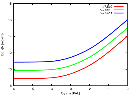
Fig. 25: As for Fig. 24 but over O₂ vmr instead of geological time $t_{\rm{geo}}$.

Results in Fig. 24 can also be plotted over O₂ mixing ratio, see Fig. 25 suggesting that one level of net primary productivity from oxygenic photosynthesis, $N$, supports only one specific O₂ surface vmr. Please note, that the y-axis in Fig. 25 is logarithmic and in the case of low O₂ atmospheres, changes in $N$ are very small but monotonically increasing.

6.2.1 Modern Earth

Regarding the NPP from oxygenic photosynthesis, $N$, the CAB model calculates $N_{\rm{CAB}}=1.1$ Pmol O₂/yr for modern Earth at 1 PAL O₂, which is within a factor of 4 of the rather uncertain observed present value ($N_{\rm{obs}}=3.75$ Pmol O₂/yr) (see red curve in Fig. 24). The calculated organic carbon burial rate of $2.1$ Tmol O₂/yr is in the range of the rather uncertain observed value of 10 Tmol O₂/yr (Holland 1978), whereas the calculated organic carbon reservoir of $3.5\cdot 10^{20}$ mol is somewhat less than the present observed value of $1.66\cdot 10^{21}$ mol (Holland 1978). Since our study assumes steady-state, the organic carbon burial rate, $\beta(N+r)$, is equal to the weathering rate of organic carbon $wC^{\rm{org}}$.

6.2.2 Archean Earth

Modern-day oceanic NPP mostly originates at the coastlines on continental shelves because the abundances of nutrients are strongly increased due to river input. However, due to the lack of knowledge about the length of the continental boundary over time, we used the continental area instead to estimate the Archean NPP, although this assumption might be crude. If we assume that the continental area was reduced (see Taylor and McLennan (1991) for evolution models of the continental crust over Earth’s history) and the burial efficiency was probably higher in the past, then the NPP would have been reduced to 1% of the modern-day value. This estimate is calculated by assuming the following:

• only 3% of the surface of the Earth was covered by continents at 2.45 Gyrs ago (before the GOE) (Pesonen et al. 2003; Taylor and McLennan 1991) which equals about 10% of today’s continental coverage. If one assumes that the NPP is proportional to the continental area then this leads to a reduction of NPP by a factor of 10.

• the absolute organic carbon burial rate of about 10 Tmol/yr is rather constant over time because the fraction of volcanic carbon that is buried as organic carbon (about 20%) has not changed strongly since at least 3.0 Gyrs (see Schidlowski et al. (1983) but also Shields and Veizer (2002) for carbon isotope data from the Precambrian). Modern burial effciency of organic carbon in the ocean is about 0.2% (Berner 1982; Betts and Holland 1991) resulting in modern NPP of 5 Pmol/yr. Since the Archean burial efficiency was likely similar to that of the modern, euxinic Black Sea of about 2% (Arthur et al. 1994), the NPP should have been further decreased by a factor of 10.

For the time of the Fe deposition found from the Hamersley BIF (2.69 - 2.44 Gyr ago), the blue curve in Fig. 24 has to be considered, yielding a value of $N_{\rm{CAB}}=8.4\cdot 10^{10}$ mol O₂/yr which is less than the estimated value of $N_{\rm{archean}}=0.01\cdot N_{\rm{obs}}=3.75\cdot 10^{13}$ mol O₂/yr that was derived for the discussion points above. This large discrepancy is likely related to uncertainties, for example, in ocean circulation, length of continental shelves, etc. Unfortunately, along with these uncertainties, burial efficiency is highly indeterminate for the Archean. Furthermore, note that there exist differences between our model output and the proxy data. In the case of the O₂ concentrations, we use the upper limits (for sulfur MIF, detrital siderite) or the lower limits (for beggiota, animals, charcoal). Some initial test runs (not shown) varying the O₂ concentration in the Archean by a factor of 10 to 100 affected the NPP by only about 10%.

6.2.3 Comparison to Previous Work

It is difficult to compare the results of this study to previous box-model work by, for example, Claire et al. (2006) and Goldblatt et al. (2006), because they do not consider a full coupled atmospheric column model with climate and photochemistry. In Claire et al. (2006) and in the transient runs by Goldblatt et al. (2006), the rise of atmospheric O₂ is accompanied by a collapse in atmospheric CH₄ due to the O₂-CH₄ feedback as already described in Section 6.1.2.

Furthermore, Goldblatt et al. (2006) found a bistability in atmospheric O₂ as a result of the non-linear behavior of their CH₄ oxidation paramerization. In their Fig. 2b, a certain range in input from oxygenic photosynthesis for a constant $r$ can support two different atmospheric O₂ concentrations, for example, a low oxygen state (before the GOE) and a high oxygen state (after the GOE) due to the O₂-O₃-UV feedback. However, such bistability behavior is not observed in our work since we treat the oxidation of CH₄ as part of the atmosphere modeling, which is decoupled from the biogeochemical modeling. It was shown (see Figs. 24 and 25) that, for atmospheres before $t_{\rm{geo}}=2.25$ Gyrs ago (with surface O₂ concentrations below $10^{-4}$ PAL), rather small changes in $N$ result in different O₂ vmrs, and hence the atmosphere-surface system is very sensitive to changes in input from oxygenic photosynthesis.

7 Sensitivity Results

Sensitivity studies were performed to derive the key parameters and boundary conditions that have the strongest impact upon the behavior of the O₂ surface flux calculated by the atmospheric module of the CAB model and the corresponding biosphere response. The following scenarios were considered:

• Scenario A: here the assumed evolutionary path of O₂ is set to be constant to 10^-5 O₂ vmr before 2.5 Gyrs ago. $S(t)$ and volcanic and metamorphic outgassing remain as for the control scenario;

• crustal mineral redox buffer:

  • Scenario B: more reduced: $\Delta f_{\rm{O}_{2}}=-1$ (QFM-1),

  • Scenario C: more oxidized: $\Delta f_{\rm{O}_{2}}=+1$ (QFM+1);

• heat flow:

  • Scenario D: $2Q$,

  • Scenario E: $0.5Q$;

• Scenario F: eddy diffusion profile is set constant to $K(z)=10^{5}$ cm² $s^{-1}$ (Kuhn and Atreya 1979) (control run: $K(z)$ from Massie and Hunten 1981);

• Scenario G: surface CO₂ concentration: 5 PAL CO₂ (sediment data place an upper limit of 10-100 PAL, see Rye et al. 1995; Sheldon 2006; Hessler et al. 2004 but see also Rosing et al. 2010 for a more conservative limit);

• Scenario H: doubled CH₄ surface flux (control scenario: 474 Tg CH₄/yr)

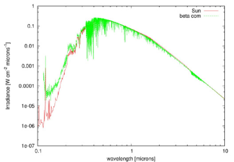
Fig. 26: Normalized stellar spectrum of $\beta$ Com (green) in comparison to the spectrum of the Sun (red) by Gueymard (2004).

• Scenario I: incident stellar radiation: young sun analog star $\beta$ Com (see Fig. 26 for comparison of stellar spectra of $\beta$ Com and the Sun)

• Scenario J: Pasteur point: lowered to $10^{-5}$ PAL O₂ (Stolper et al. 2010);

• Scenario K: solubility of O₂ in ocean water:
  Henry’s law constant $H_{\rm{O}_{2}}=9.8\cdot 10^{-4}$ M/atm (Broecker and Peng, 1982) at 25^∘C, from the diffusion coefficient $K_{\rm{diffusion,O_{2}}}=2.26\cdot 10^{-5}$ cm²/s at 25^∘C (Broecker and Peng, 1974) one can calculate a piston velocity as $\rm{v}_{p}(\rm{O}_{2})=5.65\cdot 10^{-3}$ cm s^-1.

In the case of Scenario A (not shown), only a minor increase in O₂ surface flux before 2.5 Gyrs ago compared to the control scenario (with a maximum relative change of 0.6%) is found. Hence atmospheric chemistry is not strongly affected compared to the scenario discussed in the previous sections (control run). The effect upon the biosphere response is a little larger. To maintain a constant O₂ vmr of $10^{-5}$ at the surface, $N$ increases by about 12 % compared to the control scenario because of the slightly enhanced O₂ surface flux.

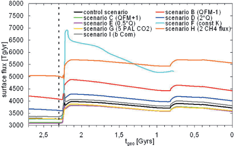
Fig. 27: Calculated atmospheric O₂ surface flux as a function of geological time $t_{\rm{geo}}$ for a number of different parameter studies compared to the control scenario described in Section 5: scenario B (QFM-1), scenario C (QFM+1), scenario D ($2Q$), scenario E ($0.5Q$), scenario F (const. $K(z)$), scenario G (5 PAL CO₂), scenario H (2 CH₄ flux) and scenario I ($\beta$ Com). The parameter studies concerning the Pasteur point (scenario J) and the ocean solubility (scenario K) have the same atmospheric O₂ surface flux as the control scenario. The beginning of the GOE at $t_{\rm{geo}}=2.3$ Gyrs is indicated as a vertical dashed line.

Fig. 27 shows how the atmospheric O₂ surface flux responds for the other sensitivity runs. A larger O₂ surface flux is needed to maintain the O₂ surface vmr in the cases of scenario B (QFM-1), scenario D ($2Q$), and scenario H (doubled CH₄ flux) because of the increased amount of reduced gases emitted at the surface.

In the case of scenario F (const. eddy diffusion), the constant $K(z)$-profile leads to a stronger O₃ layer (not shown) with an O₃ column amount of about 430 DU at $t_{\rm{geo}}=2.18$ Gyrs ago (0.1 PAL O₂ - cf. 263 DU for control run). Furthermore, the O₃ surface vmr of $1.2\cdot 10^{-7}$ is higher than that in the control scenario ($2.61\cdot 10^{-8}$) (not shown). At 0.1 PAL O₂, eddy diffusion is greatly increased compared to modern Earth above 10 km, which leads to a more efficient transport of chemical species toward lower pressure, and hence species such as CH₄ and N₂O are more quickly removed. HO_x and NO_x are weaker, resulting in enhanced O₃ abundances. Hence, the overall increased O₃ abundances result in increased O₂ surface fluxes after the GOE because the production of O₃ is an effective sink for O₂. In the case of scenario I ($\beta$ Com), a slightly increased O₂ surface flux is calculated, which is also a direct consequence of the increased O₃ abundance in such an atmosphere. Due to enhanced UV radiation emitted by the star below about 300 nm, the production of O₃ via the Chapman mechanism, which represents a loss process for O₂, is stimulated. The O₂ surface flux is generally lower for scenario C (QFM+1) and scenario E ($0.5Q$) because less reduced chemical species are emitted into the atmosphere. In the case of scenario G (5 PAL CO₂,) the O₂ fluxes at the surface are less than that in the control scenario after the GOE, which implies that increased CO₂ concentrations lead to higher production of O₂ in the atmosphere because CO₂ photolysis is a source for O and O(¹D) and, hence, O₂. Before the GOE, O₂ fluxes are equal to the control scenario.

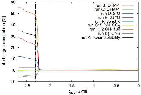
Fig. 28: Calculated relative change in % of the input from oxygenic photosynthesis, $N$, for the different parameter changes compared to the control scenario as a function of geological time $t_{\rm{geo}}$. Scenario J is not shown in this figure. The beginning of the GOE at $t_{\rm{geo}}=2.3$ Gyrs is indicated as a vertical dashed line.

The effect upon the biosphere is shown in Fig. 28. For the different scenarios we find:

• Scenario B (QFM-1, red): Due to the overall, more reduced atmospheric conditions and the associated destruction of O₂, a higher O₂ surface flux is required, and hence a higher $N$ is needed, which results in a rel. change of about 29% at 2.7 Gyrs ago;

• Scenario C (QFM+1, green dashed): More oxidized conditions due to less reduced gases emitted at the surface lead to a maximum decrease of 5 % in $N$;

• Scenario D ($2Q$, blue dotted): A doubled heat flow results in more reduced gases and, hence, an overall increase in $N$ by 12 %;

• Scenario E ($0.5Q$, magenta): A smaller heat flow yields a decrease in $N$ by about 6%;

• Scenario F (const. $K(z)$, cyan): There are only minor relative changes with a maximum of 2-3% at 2.22 Gyrs ago;

• Scenario G (5 PAL CO₂, yellow): Minor relative changes are observed with a minimum value of 2% at 2.24 Gyrs; after the GOE, the relative change increases to 1-2%, which reflects the higher surface pressures and temperatures compared to the control run;

• Scenario H (2 CH₄ flux, orange): A doubled CH₄ flux at the surface has a strong effect on the biosphere response and results in a maximum relative change of 55 % in $N$;

• Scenario I ($\beta$ Com, grey): A higher UV radiation below 300 nm results in a larger O₃ column and, hence, a higher O₂ surface flux and therefore an increase in $N$ by about 4%;

• Scenario K: (ocean solubility, green): To maintain the same O₂ flux as for the control run, the aqueous concentration $[\rm{O}_{2}]^{\rm{aq}}$ and, hence, $N$ must increase because the solubility constant and piston velocity of O₂ are lower (see Eq. 13), a maximum increase of 35% is observed;

• Scenario J (Pasteur point, not shown in Fig. 28): In the case of the reduction of the Pasteur point, O₂ can be consumed by aerobic respiration down to lower aqueous O₂ concentrations which results in a stronger O₂ loss, and therefore the input from oxygenic photosynthesis must increase by several orders of magnitude (10³). Hence, better knowledge of the Pasteur point is important.

Generally speaking, relative changes in $N$ (except for the Pasteur point run) are very small after the GOE, although the corresponding O₂ surface fluxes calculated by the atmospheric chemistry module are increased or decreased in comparison to the control scenario (see Fig. 27). This is because, in the regime after the GOE, it is the partial pressure of O₂, and hence surface conditions ($p_{\rm{surf}}$, $T_{\rm{surf}}$), rather than the O₂ surface flux reflecting the chemical behavior of O₂ in the atmosphere (as discussed in Section 6.2) which is responsible for the biosphere response.

8 Conclusion

This is the first study to our knowledge that includes the coupling between geological, biological, and (detailed) atmospheric climate and photochemistry processes. By applying our unique global-mean atmospheric column module with interactive O₂, CO₂, and N₂ (CAB model) which can respond to detailed atmospheric chemistry and radiative transfer, our study investigated consistently chemical and biological sources and sinks that controll the evolution of atmospheric O₂ on Earth and potentially on Earth-like extrasolar planets. Our new model reasonably reproduces observations of the modern Earth for both atmospheric data (atmospheric chemical species, climate) and biological-geological data (net primary productivity and burial). Our results suggest that, in the atmosphere, CO₂ (we assume modern-day surface values) is not an isoprofile (as is commonly assumed in the literature) in the middle atmosphere for all early Earth analog runs, and O₂ is no longer an isoprofile for runs with less than $10^{-4}$ O₂ surface vmrs.

The O₂ bistability found by Goldblatt et al. (2006) is not observed in our calculations due to our consistent atmospheric treatment of CH₄ oxidation. Furthermore, we calculate an increase in CH₄ concentration with increasing O₂ vmrs during the GOE in contrast to previous works (e.g., Claire et al. 2006; Zahnle et al. 2006) with much simpler chemical schemes, which have suggested the opposite effect. Important caveats, however, include uncertainties, for example, in the modeled temperature evolution due to lacking knowledge about the evolution of greenhouse gas evolution (CO₂, CH₄, N₂O) as well as missing processes in the model, for example, the response of methanogen activity to changing atmospheric O₂(g) and temperature.

For the first time, we applied the Pathway Analysis Program for O₂ in the early Earth analog atmosphere and found that photolysis of CO₂ is an important abiotic source of O₂ (and CO) in the upper atmosphere. However, this process is not able to change the overall atmospheric O₂ content on early Earth analog planets. In the early reducing atmosphere, O₂ is mainly destroyed via oxidation of CO, CH₄, and H₂ in the lower atmosphere. It was found that CO is a crucial chemical species in chemical pathways that produce and destroy O₂.

On applying the CAB model to the early Earth analog atmospheres, we calculated O₂ surface fluxes over the geological timescales. An important result was that different types of atmospheres, that is, with different oxidizing natures, could be supported by one O₂ surface flux respectively. More work is required to understand the nature of the oxidizing-reducing feedbacks in the early Earth analog atmospheres. But due to the coupling of biogeochemical processes to the atmosphere we found that there is only one net primary productivity from oxygenic photosynthesis that is needed to maintain the O₂ surface vmr for every type of atmosphere considered. The atmospheric O₂ surface flux is most sensitive to changes in the biogenic CH₄ surface emission and a crustal chemical redox buffer that emits more reduced than oxidized gases (QFM-1), but also to the assumed eddy diffusion profile. Atmospheres with enhanced CO₂ concentrations lead to a decrease in the required atmospheric O₂ surface flux. The net primary productivity of the biosphere is strongly influenced by changes in the Pasteur point, biogenic CH₄ surface emission, ocean solubility, and crustal chemical redox buffers that emit more reduced gases (QFM-1), and hence resolving the uncertainties in these quantities are crucial for a better understanding of early Earth analog atmospheres.

Although our main focus was on early Earth analog planets it is nevertheless instructive to briefly discuss our results in an Earth-like exoplanetary context. Clearly this discussion remains hypothetical and requires future work. Regarding Earth-like extrasolar planets, results suggest that different atmospheric ”states” of O₂ could exist even for similar biomass output. The PAP analysis suggests that atmospheres where volatile organic compounds build up atmospheric O₂ are disfavored due to oxidation reactions. Furthermore, extrasolar Earth-like planets with strong interior outgassing of reducing gases can lead to so-called false negatives for O₂ (e.g., PAP results show that CO and/or CH₄ containing pathways destroy O₂ and, hence, mask the existence of O₂ producing biospheres). Since all O₂ destruction pathways found feature HO_x, steamy high UV exoatmospheres could also lead to similar false negatives in O₂. Extrasolar Earth-like planets with strong mixing (e.g. due to a weak temperature inversion) have a potentially strong positive effect on atmospheric O₃. Varying key parameters (e.g., interior outgassing) in low O₂ containing exoatmospheres ($<1\%$ PAL) significantly impacts the net productivity of a potential biosphere for a given surface O₂ concentration.

Acknowledgments:
This research was supported by the Helmholtz Gemeinschaft through the research alliance ”Planetary Evolution and Life”.

This study has received financial support from the French State in the frame of the ”Investments for the future” Programme IdEx Bordeaux, reference ANR-10-IDEX-03-02.

M. Godolt acknowledges funding by the Helmholtz Foundation via the Helmholtz Postdoc Project ”Atmospheric dynamics and photochemistry of Super-Earth planets”.

This work was partially funded by grant AyA 2012 32237 awarded by the Spanish Ministerio 353 de Economia y Competitividad.

The authors thank the unknown referee for his/her valuable comments.

Author Disclosure Statement:
No competing financial interests exist.

Tab. 1: Present-day fluxes of volcanic gases considered in the photochemistry module. Fluxes are given in Teragrams (Tg ($10^{12}$ g))/yr.

species i	flux $P_{\rm{volc,i}}^{\rm{now}}$ [Tg/yr]	reference
H2	9.6	Holland (2002)
H2S	1.4	Halmer (2002)
SO2	15	Halmer (2002)
CO	1.5	Zahnle et al. (2006)
CH4	4	Kvenvolden and Rogers (2005)
CO2	367	Mörner and Etiope (2002)

Tab. 2: Processes of the marine biosphere after Goldblatt et al. (2006). Organic carbon is represented by CH₂O.

Process name	Reaction
anoxygenic	4Fe2+ + CO2 + 11H2 + h$\nu$ $\rightarrow$
photosynthesis	4Fe(OH)3 + CH2O + 8H+
oxygenic photosynthesis	CO2 +H2O + h$\nu$ $\rightarrow$ CH2O + O2
aerobic respiration	CH2O + O2 $\rightarrow$ CO2 + H2O
acetotrophic methanogenic	2CH2O $\rightarrow$ CH3COOH
fermentation	CH3COOH $\rightarrow$ CH4 + CO2
methanotrophic	CH4 + 2 O2 $\rightarrow$ CO2 + 2H2O
anaerobic respiration

Tab. 3: Relative change of relevant chemical species profiles against RG2011 over altitude.

species	relative change $X$ [%]
O3	-0.7 to 3.5
H2O	-2.2 to 0.3
CH4	0.3 to 1.2
N2O	-1.7 to 0.2
CH3Cl	0.0 to 2.7
CO2	0.0 to 0.6

Tab. 4: Column amount [DU] (Dobson unit, $2.69\cdot 10^{16}$ molecules cm^-2) of selected chemical species for modern Earth calculated by the CAB model and RG2011.

species	CAB model	RG2011	relative change $X$ [%]
O3	305.0	304.7	0.1
H2O	$2.418\cdot 10^{6}$	$2.428\cdot 10^{6}$	-0.4
CH4	1237	1233	0.3
N2O	230.5	231.3	-0.3
CH3Cl	0.358	0.358	0.0

Tab. 5: Assumed O₂ evolution in this work for early Earth analog atmospheres. The surface O₂ concentration is derived from the possible evolutionary path of O₂ by Catling and Claire (2005) (see Fig. 3). The geological time $t_{\rm{geo}}$ is interpolated from O${}_{2}(t_{\rm{geo}})$.

eon	$t_{\rm{geo}}$ [Gyrs]	surface O2 [PAL]
Phanerozoic	0.0	1.0
	0.39	$9.05\cdot 10^{-1}$
	0.41	$8.50\cdot 10^{-1}$
	0.52	$7.14\cdot 10^{-1}$
Paleozoic	0.73	$5.50\cdot 10^{-1}$
	0.78	$4.10\cdot 10^{-1}$
	0.81	$3.00\cdot 10^{-1}$
	0.82	$2.50\cdot 10^{-1}$
	0.83	$2.00\cdot 10^{-1}$
	1.01	$1.64\cdot 10^{-1}$
	1.21	$1.64\cdot 10^{-1}$
	1.41	$1.64\cdot 10^{-1}$
	1.63	$1.64\cdot 10^{-1}$
	1.80	$1.64\cdot 10^{-1}$
	2.13	$1.43\cdot 10^{-1}$
	2.18	$1.00\cdot 10^{-1}$
	2.21	$5.50\cdot 10^{-2}$
	2.22	$2.50\cdot 10^{-2}$
	2.22	$1.43\cdot 10^{-2}$
	2.22	$1.00\cdot 10^{-2}$
	2.23	$5.50\cdot 10^{-3}$
	2.23	$2.50\cdot 10^{-3}$
	2.24	$1.43\cdot 10^{-3}$
	2.24	$1.00\cdot 10^{-3}$
	2.25	$5.50\cdot 10^{-4}$
	2.25	$2.50\cdot 10^{-4}$
	2.27	$1.43\cdot 10^{-4}$
	2.28	$1.00\cdot 10^{-4}$
	2.32	$5.50\cdot 10^{-5}$
Archean	2.55	$2.50\cdot 10^{-5}$
	2.58	$1.43\cdot 10^{-5}$
	2.59	$1.00\cdot 10^{-5}$
	2.60	$5.50\cdot 10^{-6}$
	2.65	$2.50\cdot 10^{-6}$
	2.68	$1.43\cdot 10^{-6}$
	2.69	$1.00\cdot 10^{-6}$
	2.70	$5.50\cdot 10^{-7}$
	2.75	$2.50\cdot 10^{-7}$

Tab. 6: Summary of dominant chemical production (P) pathways of O₂ found by PAP and their percentage contribution to the total column-integrated O₂ production rate for an Earth-like atmosphere with a surface O₂ vmr of $10^{-6}$ PAL O₂. Only pathways that contribute $>1.5$% of the total column-integrated production rate are shown. For explanation of classes and subclasses see text.

class	subclass	pathway number	contribution $[\%]$	pathway
PA	PA1	P1	28.4	2$\cdot$(CO2 + h$\nu$ $\rightarrow$ CO + O(1D))
				2$\cdot$(O(1D) + N2 $\rightarrow$ O + N2)
				HO2 + O $\rightarrow$ OH + O2
				OH + O $\rightarrow$ H + O2
				H + O2 + M $\rightarrow$ HO2 + M
				net: 2CO2 $\rightarrow$ O2 + 2CO
	PA1	P2	28.1	2$\cdot$(CO2 + h$\nu$ $\rightarrow$ CO + O)
				HO2 + O $\rightarrow$ OH + O2
				OH + O $\rightarrow$ H + O2
				H + O2 + M $\rightarrow$ HO2 + M
				net: 2CO2 $\rightarrow$ O2 + 2CO
	PA1	P7	2.3	2$\cdot$(CO2 + h$\nu$ $\rightarrow$ CO + O(1D))
				2$\cdot$(O(1D) + N2 $\rightarrow$ O + N2)
				O + O2 + M $\rightarrow$ O3 + M
				OH + O $\rightarrow$ H + O2
				H + O3 $\rightarrow$ OH + O2
				net: 2CO2 $\rightarrow$ O2 + 2CO
	PA2	P3	20.7	2$\cdot$(CO2 + h$\nu$ $\rightarrow$ CO + O(1D))
				2$\cdot$(O(1D) + N2 $\rightarrow$ O + N2)
				O + O + M $\rightarrow$ O2 + M
				net: 2CO2 $\rightarrow$ O2 + 2CO
	PA2	P4	6.8	2$\cdot$(CO2 + h$\nu$ $\rightarrow$ CO + O)
				O + O + M $\rightarrow$ O2 + M
				net: 2CO2 $\rightarrow$ O2 + 2CO
PB	PB1	P6	3.9	OH + O $\rightarrow$ H + O2
				H + O2 + M $\rightarrow$ HO2 + M
				HO2 + O $\rightarrow$ OH + O2
				net: 2O $\rightarrow$ O2
	PB2	P5	5.3	O + O + M $\rightarrow$ O2 + M
				net: 2O $\rightarrow$ O2

Tab. 7: As for Tab. LABEL:proPAPpathstab but for O₂ destruction (L) pathways.

class	subclass	pathway number	contribution $[\%]$	pathway
LA	LA1	L1	28.5	2$\cdot$(H + O2 + M $\rightarrow$ HO2 + M)
				HO2 + HO2 $\rightarrow$ H2O2 + O2
				H2O2 + h$\nu$ $\rightarrow$ OH + OH
				2$\cdot$(CO + OH $\rightarrow$ CO2 + H)
				net: O2 + 2CO $\rightarrow$ 2CO2
	LA1	L2	9.4	2$\cdot$(H + O2 + M $\rightarrow$ HO2 + M)
				HO2 + O $\rightarrow$ OH + O2
				HO2 + h$\nu$ $\rightarrow$ OH + O
				2$\cdot$(CO + OH $\rightarrow$ CO2 + H)
				net: O2 + 2CO $\rightarrow$ 2CO2
	LA1	L6	4.4	2$\cdot$(H + O2 + M $\rightarrow$ HO2 + M)
				HO2 + O $\rightarrow$ OH + O2
				NO + HO2 $\rightarrow$ NO2 + OH
				2$\cdot$(CO + OH $\rightarrow$ CO2 + H)
				NO2 + h$\nu$ $\rightarrow$ NO + O
				net: O2 + 2CO $\rightarrow$ 2CO2
	LA1	L8	3.4	H + O2 + M $\rightarrow$ HO2 + M
				H + HO2 $\rightarrow$ OH + OH
				2$\cdot$(CO + OH $\rightarrow$ CO2 + H)
				net: O2 + 2CO $\rightarrow$ 2CO2
	LA2	L3	7.4	O2 + h$\nu$ $\rightarrow$ O + O
				2$\cdot$(HO2 + O $\rightarrow$ OH + O2)
				2$\cdot$(CO + OH $\rightarrow$ CO2 + H)
				2$\cdot$(H + O2 + M $\rightarrow$ HO2 + M)
				net: O2 + 2CO $\rightarrow$ 2CO2
	LA2	L5	5.0	O2 + h$\nu$ $\rightarrow$ O + O(1D)
				O(1D) + N2 $\rightarrow$ O + N2
				2$\cdot$(HO2 + O $\rightarrow$ OH + O2)
				2$\cdot$(CO + OH $\rightarrow$ CO2 + H)
				2$\cdot$(H + O2 + M $\rightarrow$ HO2 + M)
				net: O2 + 2CO $\rightarrow$ 2CO2
LB	LB1	L4	5.4	H2O2 + h$\nu$ $\rightarrow$ OH + OH
				2$\cdot$(CH4 + OH $\rightarrow$ CH3 + H2O)
				2$\cdot$(CH3 + O2 + M $\rightarrow$ CH3O2 + M)
				2$\cdot$(CH3O2 + HO2 $\rightarrow$ CH3OOH + O2)
				2$\cdot$(CH3OOH + h$\nu$ $\rightarrow$ H3CO + OH)
				2$\cdot$(H2CO + OH $\rightarrow$ H2O + HCO)
				2$\cdot$(HCO + O2 $\rightarrow$ HO2 + CO)
				HO2 + HO2 $\rightarrow$ H2O2 + O2
				2$\cdot$(H3CO + O2 $\rightarrow$ H2CO + HO2)
				net: 3O2 + 2CH4 $\rightarrow$ 4H2O + 2CO
	LB1	L7	4.3	2$\cdot$(H2CO + OH $\rightarrow$ H2O + HCO)
				2$\cdot$(HCO + O2 $\rightarrow$ HO2 + CO)
				3$\cdot$(HO2 + HO2 $\rightarrow$ H2O2 + O2)
				3$\cdot$(H2O2 + h$\nu$ $\rightarrow$ OH + OH)
				2$\cdot$(CH4 + OH $\rightarrow$ CH3 + H2O)
				2$\cdot$(CH3 + O2 + M $\rightarrow$ CH3O2 + M)
				2$\cdot$(CH3O2 + OH $\rightarrow$ H3CO + HO2)
				2$\cdot$(H3CO + O2 $\rightarrow$ H2CO + HO2)
				net: 3O2 + 2CH4 $\rightarrow$ 4H2O + 2CO
	LB2	L10	2.5	CH3OOH + h$\nu$ $\rightarrow$ H3CO + OH
				CH4 + OH $\rightarrow$ CH3 + H2O
				CH3 + O2 + M $\rightarrow$ CH3O2 + M
				CH3O2 + HO2 $\rightarrow$ CH3OOH + O2
				H3CO + O2 $\rightarrow$ H2CO + HO2
				H2CO + h$\nu$ $\rightarrow$ H2 + CO
				net: O2 + CH4 $\rightarrow$ H2O + H2 + CO
LC		L9	3.0	2$\cdot$(H + O2 + M $\rightarrow$ HO2 + M)
				HO2 + HO2 $\rightarrow$ H2O2 + O2
				H2O2 + h$\nu$ $\rightarrow$ OH + OH
				2$\cdot$(H2 + OH $\rightarrow$ H2O + H)
				net: O2 + 2H2 $\rightarrow$ 2H2O
LD		L11	1.7	CO + OH $\rightarrow$ CO2 + H
				H2O + h$\nu$ $\rightarrow$ H + OH
				2$\cdot$(H + O2 + M $\rightarrow$ HO2 + M)
				HO2 + HO2 $\rightarrow$ H2O2 + O2
				net: O2 + H2O + CO $\rightarrow$ H2O2 + CO2

References

- Allen et al. (1984) Allen, M., J. I. Lunine, and Y. L. Yung (1984), The vertical distribution of ozone in the mesosphere and lower thermosphere, Journal of Geophysical Research: Atmospheres, 89(D3), 4841–4872.
- Antoine et al. (1996) Antoine, D., J.-M. André, and A. Morel (1996), Oceanic primary production: 2. estimation at global scale from satellite (coastal zone color scanner) chlorophyll, Global Biogeochemical Cycles, 10(1), 57–69, doi:10.1029/95GB02832.
- Arthur et al. (1994) Arthur, M. A., W. E. Dean, E. D. Neff, B. J. Hay, J. King, and G. Jones (1994), Varve calibrated records of carbonate and organic carbon accumulation over the last 2000 years in the black sea, Global Biogeochemical Cycles, 8(2), 195–217.
- Bates and Nicolet (1950) Bates, D. R., and M. Nicolet (1950), The photochemistry of atmospheric water vapor, Journal of Geophysical Research, 55(3), 301–327.
- Berkner and Marshall (1965) Berkner, L. V., and L. C. Marshall (1965), On the Origin and Rise of Oxygen Concentration in the Earth’s Atmosphere., Journal of Atmospheric Sciences, 22, 225–261.
- Berner (1982) Berner, R. A. (1982), Burial of organic carbon and pyrite sulfur in the modern ocean; its geochemical and environmental significance, American Journal of Science, 282(4), 451–473.
- Berner et al. (2000) Berner, R. A., S. T. Petsch, J. A. Lake, D. J. Beerling, B. N. Popp, R. S. Lane, E. A. Laws, M. B. Westley, N. Cassar, F. I. Woodward, and W. P. Quick (2000), Isotope Fractionation and Atmospheric Oxygen: Implications for Phanerozoic O2 Evolution, Science, 287, 1630–1633.
- Betts and Holland (1991) Betts, J. N., and H. D. Holland (1991), The oxygen content of ocean bottom waters, the burial efficiency of organic carbon, and the regulation of atmospheric oxygen, Global and Planetary Change, 5(1-2), 5 – 18, atmospheric Oxygen Variation Through Geologic Time.
- Brent (1971) Brent, R. P. (1971), An algorithm with guaranteed convergence for finding a zero of a function, The Computer Journal, 14(4), 422–425.
- Canfield (2005) Canfield, D. E. (2005), THE EARLY HISTORY OF ATMOSPHERIC OXYGEN: Homage to Robert M. Garrels, Annual Review of Earth and Planetary Sciences, 33, 1–36.
- Canfield and Teske (1996) Canfield, D. E., and A. Teske (1996), Late Proterozoic rise in atmospheric oxygen concentration inferred from phylogenetic and sulphur-isotope studies, Nature, 382, 127–132.
- Catling and Claire (2005) Catling, D. C., and M. W. Claire (2005), How Earth’s atmosphere evolved to an oxic state: A status report, Earth and Planetary Science Letters, 237, 1–20.
- Chaloner (1989) Chaloner, W. G. (1989), Fossil charcoal as an indicator of palaeoatmospheric oxygen level, Journal of the Geological Society, 146(1), 171–174.
- Chapman (1930) Chapman, S. (1930), A Theory of Upper-Atmospheric Ozone, Memoirs of the Royal Meteorological Society, 3, 103–125.
- Charbonneau et al. (2009) Charbonneau, D., Z. K. Berta, J. Irwin, C. J. Burke, P. Nutzman, L. A. Buchhave, C. Lovis, X. Bonfils, D. W. Latham, S. Udry, R. A. Murray-Clay, M. J. Holman, E. E. Falco, J. N. Winn, D. Queloz, F. Pepe, M. Mayor, X. Delfosse, and T. Forveille (2009), A super-Earth transiting a nearby low-mass star, Nature, 462, 891–894.
- Charnay et al. (2013) Charnay, B., F. Forget, R. Wordsworth, J. Leconte, E. Millour, F. Codron, and A. Spiga (2013), Exploring the faint young Sun problem and the possible climates of the Archean Earth with a 3-D GCM, Journal of Geophysical Research (Atmospheres), 118, 10,414.
- Christensen (1985) Christensen, U. R. (1985), Thermal evolution models for the earth, Journal of Geophysical Research: Solid Earth, 90(B4), 2995–3007.
- Claire et al. (2006) Claire, M. W., D. C. Catling, and K. J. Zahnle (2006), Biogeochemical modelling of the rise in atmospheric oxygen, Geobiology, 4(4), 239–269.
- Cloud (1968) Cloud, P. E., Jr. (1968), Atmospheric and Hydrospheric Evolution on the Primitive Earth, Science, 160, 729–736.
- Crutzen (1970) Crutzen, P. J. (1970), The influence of nitrogen oxides on the atmospheric ozone content, Quarterly Journal of the Royal Meteorological Society, 96(408), 320–325.
- Engelhardt (1974) Engelhardt, W. (1974), On the dual role of respiration, Molecular and Cellular Biochemistry, 5(1-2), 25–33, doi:10.1007/BF01874169.
- Evans et al. (1968) Evans, W. F. J., D. M. Hunten, E. J. Llewellyn, and A. V. Jones (1968), Altitude profile of the infrared atmospheric system of oxygen in the dayglow, Journal of Geophysical Research, 73(9), 2885–2896.
- Farquhar et al. (2000) Farquhar, J., J. Savarino, T. L. Jackson, and M. H. Thiemens (2000), Evidence of atmospheric sulphur in the martian regolith from sulphur isotopes in meteorites, Nature, 404, 50–52.
- Frost (1991) Frost, B. R. (1991), Introduction to oxygen fugacity and its petrologic importance, Reviews in Mineralogy and Geochemistry, 25(1), 1–9.
- Giorgi and Chameides (1985) Giorgi, F., and W. L. Chameides (1985), The rainout parameterization in a photochemical model, J. Geophys. Res., 90, 7872–7880.
- Goldblatt et al. (2006) Goldblatt, C., T. M. Lenton, and A. J. Watson (2006), Bistability of atmospheric oxygen and the Great Oxidation, Nature, 443, 683–686.
- Goldblatt et al. (2009) Goldblatt, C., M. W. Claire, T. M. Lenton, A. J. Matthews, A. J. Watson, and K. J. Zahnle (2009), Nitrogen-enhanced greenhouse warming on early Earth, Nature Geoscience, 2, 891–896.
- Gough (1981) Gough, D. O. (1981), Solar interior structure and luminosity variations, Solar Physics, 74, 21–34.
- Grenfell et al. (2006) Grenfell, J. L., R. Lehmann, P. Mieth, U. Langematz, and B. Steil (2006), Chemical reaction pathways affecting stratospheric and mesospheric ozone, Journal of Geophysical Research (Atmospheres), 111, D17311.
- Grenfell et al. (2007a) Grenfell, J. L., B. Stracke, P. von Paris, B. Patzer, R. Titz, A. Segura, and H. Rauer (2007a), The response of atmospheric chemistry on earthlike planets around F, G and K Stars to small variations in orbital distance, Planet. Space Science, 55, 661–671.
- Grenfell et al. (2007b) Grenfell, J. L., J.-M. Grießmeier, B. Patzer, H. Rauer, A. Segura, A. Stadelmann, B. Stracke, R. Titz, and P. Von Paris (2007b), Biomarker Response to Galactic Cosmic Ray-Induced NOx And The Methane Greenhouse Effect in The Atmosphere of An Earth-Like Planet Orbiting An M Dwarf Star, Astrobiology, 7, 208–221.
- Grenfell et al. (2011) Grenfell, J. L., S. Gebauer, P. von Paris, M. Godolt, P. Hedelt, A. B. C. Patzer, B. Stracke, and H. Rauer (2011), Sensitivity of biomarkers to changes in chemical emissions in the Earths Proterozoic atmosphere, Icarus, 211, 81–88.
- Grenfell et al. (2012) Grenfell, J. L., J.-M. Grießmeier, P. von Paris, A. B. C. Patzer, H. Lammer, B. Stracke, S. Gebauer, F. Schreier, and H. Rauer (2012), Response of Atmospheric Biomarkers to NOx-Induced Photochemistry Generated by Stellar Cosmic Rays for Earth-like Planets in the Habitable Zone of M Dwarf Stars, Astrobiology, 12, 1109–1122.
- Grenfell et al. (2013) Grenfell, J. L., S. Gebauer, M. Godolt, K. Palczynski, H. Rauer, J. Stock, P. von Paris, R. Lehmann, and F. Selsis (2013), Potential Biosignatures in Super-Earth Atmospheres II. Photochemical Responses, Astrobiology, 13, 415–438.
- Gueymard (2004) Gueymard, C. A. (2004), The sun’s total and spectral irradiance for solar energy applications and solar radiation models, Solar Energy, 76(4), 423–453.
- Haagen-Smit (1952) Haagen-Smit, A. J. (1952), Chemistry and Physiology of Los Angeles Smog, Ind. Eng. Chem., 44(6), 1342–1346.
- Halmer (2002) Halmer, M. (2002), The annual volcanic gas input into the atmosphere, in particular into the stratosphere: a global data set for the past 100 years, Journal of Volcanology and Geothermal Research, 115, 511–528.
- Haqq-Misra et al. (2011) Haqq-Misra, J., J. F. Kasting, and S. Lee (2011), Availability of O2 and H2O2 on Pre-Photosynthetic Earth, Astrobiology, 11, 293–302.
- Hays and Roble (1973) Hays, P., and R. Roble (1973), Observation of mesospheric ozone at low latitudes, Planetary and Space Science, 21(2), 273 – 279.
- Hessler et al. (2004) Hessler, A. M., D. R. Lowe, R. L. Jones, and D. K. Bird (2004), A lower limit for atmospheric carbon dioxide levels 3.2 billion years ago, Nature, 428, 736–738.
- Holland (1978) Holland, H. D. (1978), The chemistry of the atmosphere and oceans / Heinrich D. Holland, xiv, 351 p. : pp., Wiley, New York :.
- Holland (1984) Holland, H. D. (1984), The chemical evolution of the atmosphere and oceans.
- Holland (2002) Holland, H. D. (2002), Volcanic gases, black smokers, and the great oxidation event, Geochimica et Cosmochimica Acta, 66, 3811–3826.
- Holland (2003) Holland, H. D. (2003), Discussion of the article by a. c. lasaga and h. ohmoto on the oxygen geochemical cycle: Dynamics and stability, geochim. cosmochim. acta 66, 361 381, 2002, Geochim. Cosmochim. Acta, 67(4), 787 – 789.
- Holland (2006) Holland, H. D. (2006), The oxygenation of the atmosphere and oceans, Philosophical Transactions of the Royal Society B: Biological Sciences, 361(1470), 903–915.
- Holland and Yang (2001) Holland, H. D., and W. Yang (2001), Toward an Explanation for the Great Oxidation Event Between ca. 2.3 and 2.0, in Eleventh Annual V. M. Goldschmidt Conference, p. 3094.
- IPCC (2001) IPCC (Ed.) (2001), Climate change 2001:The Scientific Basis: Contribution of Working Group I to the third assessment report of the Intergovernmental Panel on Climate Change, Cambridge University Press, Cambridge and , New York.
- Isley and Abbott (1999) Isley, A. E., and D. H. Abbott (1999), Plume-related mafic volcanism and the deposition of banded iron formation, J. Geophys. Res., 104, 15,461–15,477.
- Jacob (1999) Jacob, D. J. (1999), Introduction to Atmospheric Chemistry, Princeton Univ., Princeton, NJ.
- Kaltenegger and Sasselov (2010) Kaltenegger, L., and D. Sasselov (2010), Detecting Planetary Geochemical Cycles on Exoplanets: Atmospheric Signatures and the Case of SO2, Astrophys. J., 708, 1162–1167.
- Kasting (1993) Kasting, J. (1993), Earth’s early atmosphere, Science, 259(5097), 920–926.
- Kasting (1982) Kasting, J. F. (1982), Stability of ammonia in the primitive terrestrial atmosphere, J. Geophys. Res., 87, 3091–3098.
- Kasting (1988) Kasting, J. F. (1988), Runaway and moist greenhouse atmospheres and the evolution of earth and venus, Icarus, 74(3), 472 – 494.
- Kasting and Catling (2003) Kasting, J. F., and D. Catling (2003), Evolution of a habitable planet, Annual Review of Astronomy and Astrophysics, 41(1), 429–463.
- Kasting and Donahue (1980) Kasting, J. F., and T. M. Donahue (1980), The evolution of atmospheric ozone, J. Geophys. Res., 85, 3255–3263.
- Kasting and Donahue (1981) Kasting, J. F., and T. M. Donahue (1981), Evolution of Oxygen and Ozone in Earths Atmosphere, in Life in the Universe, edited by J. Billingham, p. 149.
- Kasting et al. (1984) Kasting, J. F., J. B. Pollack, and D. Crisp (1984), Effects of high CO2 levels on surface temperature and atmospheric oxidation state of the early earth, Journal of Atmospheric Chemistry, pp. 403–428.
- Kasting et al. (1985) Kasting, J. F., H. D. Holland, and J. P. Pinto (1985), Oxidant abundances in rainwater and the evolution of atmospheric oxygen, J. Geophys. Res., 901, 10,497–+.
- Kasting et al. (1993) Kasting, J. F., D. P. Whitmire, and R. T. Reynolds (1993), Habitable Zones around Main Sequence Stars, Icarus, 101, 108–128.
- Kasting et al. (1997) Kasting, J. F., D. C. B. Whittet, and W. R. Sheldon (1997), Ultraviolet radiation from F and K stars and implications for planetary habitability, Origins of Life and Evolution of the Biosphere, 27, 413–420.
- Kharecha et al. (2005) Kharecha, P., J. KASTING, and J. SIEFERT (2005), A coupled atmosphereecosystem model of the early archean earth, Geobiology, 3(2), 53–76.
- Kienert et al. (2012) Kienert, H., G. Feulner, and V. Petoukhov (2012), Faint young Sun problem more severe due to ice-albedo feedback and higher rotation rate of the early Earth, Geophys. Res. Letters, 39, L23710.
- Kitzmann et al. (2010) Kitzmann, D., A. B. C. Patzer, P. von Paris, M. Godolt, B. Stracke, S. Gebauer, J. L. Grenfell, and H. Rauer (2010), Clouds in the atmospheres of extrasolar planets. I. Climatic effects of multi-layered clouds for Earth-like planets and implications for habitable zones, Astronomy & Astrophysics, 511, A66+.
- Kitzmann et al. (2011a) Kitzmann, D., A. B. C. Patzer, P. von Paris, M. Godolt, and H. Rauer (2011a), Clouds in the atmospheres of extrasolar planets. II. Thermal emission spectra of Earth-like planets influenced by low and high-level clouds, Astronomy & Astrophysics, 531, A62+.
- Kitzmann et al. (2011b) Kitzmann, D., A. B. C. Patzer, P. von Paris, M. Godolt, and H. Rauer (2011b), Clouds in the atmospheres of extrasolar planets. III. Impact of low and high-level clouds on the reflection spectra of Earth-like planets, Astronomy & Astrophysics, 534, A63.
- Knoll and Holland (1995) Knoll, A. H., and H. D. Holland (1995), Oxygen and proterozoic evolution: an update, Effects of Past Global Change on Life, pp. 21–33.
- Kopp et al. (2005) Kopp, R. E., J. L. Kirschvink, I. A. Hilburn, and C. Z. Nash (2005), The paleoproterozoic snowball earth: A climate disaster triggered by the evolution of oxygenic photosynthesis, Proceedings of the National Academy of Sciences of the United States of America, 102(32), 11,131–11,136.
- Kuhn and Atreya (1979) Kuhn, W. R., and S. K. Atreya (1979), Ammonia photolysis and the greenhouse effect in the primordial atmosphere of the earth, Icarus, 37, 207–213.
- Kump et al. (2001) Kump, L. R., J. F. Kasting, and M. E. Barley (2001), Rise of atmospheric oxygen and the ”upside-down” Archean mantle, Geochem. Geophys. Geosyst., 2.
- Kunze et al. (2014) Kunze, M., M. Godolt, U. Langematz, J. Grenfell, A. Hamann-Reinus, and H. Rauer (2014), Investigating the early earth faint young sun problem with a general circulation model, Planetary and Space Science, 98(0), 77 – 92, planetary evolution and life.
- Kvenvolden and Rogers (2005) Kvenvolden, K. A., and B. W. Rogers (2005), Gaia’s breath - global methane exhalations, Marine and Petroleum Geology, 22(4), 579 – 590, near-Surface Hydrocarbon Migration: Mechanisms and Seepage Rates.
- Lasaga and Ohmoto (2002) Lasaga, A. C., and H. Ohmoto (2002), The oxygen geochemical cycle: dynamics and stability, Geochimica et Cosmochimica Acta, 66, 361–381.
- Leconte et al. (2013) Leconte, J., F. Forget, B. Charnay, R. Wordsworth, and A. Pottier (2013), Increased insolation threshold for runaway greenhouse processes on Earth-like planets, Nature, 504, 268–271.
- Léger et al. (2009) Léger, A., D. Rouan, J. Schneider, P. Barge, M. Fridlund, B. Samuel, M. Ollivier, E. Guenther, M. Deleuil, H. J. Deeg, M. Auvergne, R. Alonso, S. Aigrain, A. Alapini, J. M. Almenara, A. Baglin, M. Barbieri, H. Bruntt, P. Bordé, F. Bouchy, J. Cabrera, C. Catala, L. Carone, S. Carpano, S. Csizmadia, R. Dvorak, A. Erikson, S. Ferraz-Mello, B. Foing, F. Fressin, D. Gandolfi, M. Gillon, P. Gondoin, O. Grasset, T. Guillot, A. Hatzes, G. Hébrard, L. Jorda, H. Lammer, A. Llebaria, B. Loeillet, M. Mayor, T. Mazeh, C. Moutou, M. Pätzold, F. Pont, D. Queloz, H. Rauer, S. Renner, R. Samadi, A. Shporer, C. Sotin, B. Tingley, G. Wuchterl, M. Adda, P. Agogu, T. Appourchaux, H. Ballans, P. Baron, T. Beaufort, R. Bellenger, R. Berlin, P. Bernardi, D. Blouin, F. Baudin, P. Bodin, L. Boisnard, L. Boit, F. Bonneau, S. Borzeix, R. Briet, J. Buey, B. Butler, D. Cailleau, R. Cautain, P. Chabaud, S. Chaintreuil, F. Chiavassa, V. Costes, V. Cuna Parrho, F. de Oliveira Fialho, M. Decaudin, J. Defise, S. Djalal, G. Epstein, G. Exil, C. Fauré, T. Fenouillet, A. Gaboriaud, A. Gallic, P. Gamet, P. Gavalda, E. Grolleau, R. Gruneisen, L. Gueguen, V. Guis, V. Guivarc’h, P. Guterman, D. Hallouard, J. Hasiba, F. Heuripeau, G. Huntzinger, H. Hustaix, C. Imad, C. Imbert, B. Johlander, M. Jouret, P. Journoud, F. Karioty, L. Kerjean, V. Lafaille, L. Lafond, T. Lam-Trong, P. Landiech, V. Lapeyrere, T. Larqué, P. Laudet, N. Lautier, H. Lecann, L. Lefevre, B. Leruyet, P. Levacher, A. Magnan, E. Mazy, F. Mertens, J. Mesnager, J. Meunier, J. Michel, W. Monjoin, D. Naudet, K. Nguyen-Kim, J. Orcesi, H. Ottacher, R. Perez, G. Peter, P. Plasson, J. Plesseria, B. Pontet, A. Pradines, C. Quentin, J. Reynaud, G. Rolland, F. Rollenhagen, R. Romagnan, N. Russ, R. Schmidt, N. Schwartz, I. Sebbag, G. Sedes, H. Smit, M. B. Steller, W. Sunter, C. Surace, M. Tello, D. Tiphène, P. Toulouse, B. Ulmer, O. Vandermarcq, E. Vergnault, A. Vuillemin, and P. Zanatta (2009), Transiting exoplanets from the CoRoT space mission. VIII. CoRoT-7b: the first super-Earth with measured radius, Astronomy & Astrophysics, 506, 287–302.
- Lehmann (2004) Lehmann, R. (2004), An algorithm for the determination of all significant pathways in chemical reaction systems, Journal of Atmospheric Chemistry, 47, 45–78, 10.1023/B:JOCH.0000012284.28801.b1.
- Lide (1995) Lide, D. R. (1995), CRC Handbook of chemistry and physics. A ready-reference book of chemical and physical data.
- Liss and Slater (1974) Liss, P. S., and P. G. Slater (1974), Flux of Gases across the Air-Sea Interface, Nature, 247, 181–184.
- Longhurst et al. (1995) Longhurst, A., S. Sathyendranath, T. Platt, and C. Caverhill (1995), An estimate of global primary production in the ocean from satellite radiometer data, Journal of Plankton Research, 17(6), 1245–1271, doi:10.1093/plankt/17.6.1245.
- Manabe and Wetherald (1967) Manabe, S., and R. T. Wetherald (1967), Thermal Equilibrium of the Atmosphere with a Given Distribution of Relative Humidity., Journal of Atmospheric Sciences, 24, 241–259.
- Massie and Hunten (1981) Massie, S. T., and D. M. Hunten (1981), Stratospheric eddy diffusion coefficients from tracer data, Journal of Geophysical Research: Oceans, 86(C10), 9859–9868.
- Mayor et al. (2009) Mayor, M., S. Udry, C. Lovis, F. Pepe, D. Queloz, W. Benz, J.-L. Bertaux, F. Bouchy, C. Mordasini, and D. Segransan (2009), The HARPS search for southern extra-solar planets: XVIII. An Earth-mass planet in the GJ 581 planetary system, acc. in Astronomy & Astrophysics.
- McElroy and Donahue (1972) McElroy, M. B., and T. M. Donahue (1972), Stability of the Martian Atmosphere, Science, 177, 986–988.
- Mischna et al. (2000) Mischna, M. A., J. F. Kasting, A. Pavlov, and R. Freedman (2000), Influence of carbon dioxide clouds on early martian climate, Icarus, 145(2), 546 – 554.
- Mlawer et al. (1997) Mlawer, E. J., S. J. Taubman, P. D. Brown, M. J. Iacono, and S. A. Clough (1997), Radiative transfer for inhomogeneous atmospheres: RRTM, a validated correlated-k model for the longwave, J. Geophys. Res., 102, 16,663–16,682.
- Mörner and Etiope (2002) Mörner, N.-A., and G. Etiope (2002), Carbon degassing from the lithosphere, Global and Planetary Change, 33(12), 185 – 203, the global carbon cycle and its changes over glacial-interglacial cycles.
- Nair et al. (1994) Nair, H., M. Allen, A. D. Anbar, Y. L. Yung, and R. T. Clancy (1994), A photochemical model of the martian atmosphere, Icarus, 111, 124–150.
- Ohmoto (1997) Ohmoto, H. (1997), When did the Earths atmosphere become oxic?, The Geochemical News.
- Ohmoto and Kerrick (1977) Ohmoto, H., and D. M. Kerrick (1977), Devolatilization equilibria in graphitic systems, American Journal of Science, 277(8), 1013–1044.
- Parkinson and Hunten (1973) Parkinson, T. D., and D. M. Hunten (1973), Spectroscopy and aeronomy of O2 on Mars., Journal of Atmospheric Sciences, 29, 1380–1390.
- Pavlov and Kasting (2002) Pavlov, A. A., and J. F. Kasting (2002), Mass-Independent Fractionation of Sulfur Isotopes in Archean Sediments: Strong Evidence for an Anoxic Archean Atmosphere, Astrobiology, 2, 27–41.
- Pavlov et al. (2000) Pavlov, A. A., J. F. Kasting, L. L. Brown, K. A. Rages, and R. Freedman (2000), Greenhouse warming by CH4 in the atmosphere of early Earth, J. Geophys. Res., 105, 11,981–11,990.
- Pavlov et al. (2001) Pavlov, A. A., L. L. Brown, and J. F. Kasting (2001), UV shielding of NH3 and O2 by organic hazes in the Archean atmosphere, J. Geophys. Res., 106, 23,267–23,288.
- Pavlov et al. (2003) Pavlov, A. A., M. T. Hurtgen, J. F. Kasting, and M. A. Arthur (2003), Methane-rich Proterozoic atmosphere?, Geology, 31, 87–+.
- Pesonen et al. (2003) Pesonen, L., S.-. Elming, S. Mertanen, S. Pisarevsky, M. D’Agrella-Filho, J. Meert, P. Schmidt, N. Abrahamsen, and G. Bylund (2003), Palaeomagnetic configuration of continents during the proterozoic, Tectonophysics, 375(14), 289 – 324.
- Prentice et al. (2001) Prentice, I., G. Farquhar, M. Fasham, M. Goulden, M. Heimann, V. Jaramillo, H. Kheshgi, C. LeQuéré, R. Scholes, and D. W. Wallace (2001), The carbon cycle and atmospheric carbon dioxide, in Climate Change 2001: the Scientific Basis. Contributions of Working Group I to the Third Assessment Report of the Intergovernmental Panel on Climate Change, edited by J. Houghton, Y. Ding, D. Griggs, M. Noguer, P. van der Linden, X. Dai, K. Maskell, and C. Johnson, pp. 185–237, Cambridge University Press, Cambridge, UK.
- Press et al. (1993) Press, W. H., S. A. Teukolsky, W. T. Vetterling, and B. P. Flannery (1993), Numerical Recipes in FORTRAN; The Art of Scientific Computing, 2nd ed., Cambridge University Press, New York, NY, USA.
- Ratner and Walker (1972) Ratner, M. I., and J. C. G. Walker (1972), Atmospheric Ozone and the History of Life., Journal of Atmospheric Sciences, 29, 803–808.
- Rauer et al. (2011) Rauer, H., S. Gebauer, P. von Paris, J. Cabrera, M. Godolt, J. L. Grenfell, A. Belu, F. Selsis, P. Hedelt, and F. Schreier (2011), Potential biosignatures in super-Earth atmospheres. I. Spectral appearance of super-Earths around M dwarfs, Astronomy & Astrophysics, 529, A8+.
- Ren et al. (1997) Ren, T., J. A. Amaral, and R. Knowles (1997), The response of methane consumption by pure cultures of methanotrophic bacteria to oxygen, Canadian Journal of Microbiology, 43(10), 925–928.
- Ribas et al. (2005) Ribas, I., E. F. Guinan, M. Güdel, and M. Audard (2005), Evolution of the Solar Activity over Time and Effects on Planetary Atmospheres. I. High-Energy Irradiances (1-1700 Å), Astrophys. J., 622, 680–694.
- Roberson et al. (2011) Roberson, A. L., J. Roadt, I. Halevy, and J. F. Kasting (2011), Greenhouse warming by nitrous oxide and methane in the proterozoic eon, Geobiology, 9(4), 313–320.
- Rosing et al. (2010) Rosing, M. T., D. K. Bird, N. H. Sleep, and C. J. Bjerrum (2010), No climate paradox under the faint early Sun, Nature, 464, 744–747.
- Runnegar (1991) Runnegar, B. (1991), Precambrian oxygen levels estimated from the biochemistry and physiology of early eukaryotes, Global and Planetary Change, 5, 97–111.
- Rye and Holland (1998) Rye, R., and H. D. Holland (1998), Paleosols and the evolution of atmospheric oxygen; a critical review, American Journal of Science, 298(8), 621–672.
- Rye et al. (1995) Rye, R., P. H. Kuo, and H. D. Holland (1995), Atmospheric carbon dioxide concentrations before 2.2 billion years ago, Nature, 378, 603–605.
- Schidlowski et al. (1983) Schidlowski, M., J. Hayes, and I. Kaplan (1983), Isotopic inferences of ancient biochemistries- carbon, sulfur, hydrogen, and nitrogen, Earth’s earliest biosphere: Its origin and evolution(A 84-43051 21-51). Princeton, NJ, Princeton University Press, 1983,, pp. 149–186.
- Schreier and Böttger (2003) Schreier, F., and U. Böttger (2003), MIRART, a line-by-line code for infrared atmospheric radiation computations including derivatives, Atmospheric and Oceanic Optics, 16, 262–268.
- Schreier and Schimpf (2001) Schreier, F., and B. Schimpf (2001), A new efficient line-by-line code for high resolution atmospheric radiation computations incl. derivatives, in IRS 2000: Current Problems in Atmospheric Radiation, A. Deepak.
- Segura et al. (2003) Segura, A., K. Krelove, J. F. Kasting, D. Sommerlatt, V. Meadows, D. Crisp, M. Cohen, and E. Mlawer (2003), Ozone Concentrations and Ultraviolet Fluxes on Earth-Like Planets Around Other Stars, Astrobiology, 3, 689–708.
- Segura et al. (2005) Segura, A., J. F. Kasting, V. Meadows, M. Cohen, J. Scalo, D. Crisp, R. A. H. Butler, and G. Tinetti (2005), Biosignatures from Earth-Like Planets Around M Dwarfs, Astrobiology, 5, 706–725.
- Segura et al. (2007) Segura, A., V. S. Meadows, J. F. Kasting, D. Crisp, and M. Cohen (2007), Abiotic formation of O2 and O3 in high-CO2 terrestrial atmospheres, Astronomy & Astrophysics, 472, 665–679.
- Sheldon (2006) Sheldon, N. D. (2006), Precambrian paleosols and atmospheric co2 levels, Precambrian Research, 147(12), 148 – 155.
- Shields and Veizer (2002) Shields, G., and J. Veizer (2002), Precambrian marine carbonate isotope database: Version 1.1, Geochemistry, Geophysics, Geosystems, 1031.
- Sleep and Windley (1982) Sleep, N. H., and B. F. Windley (1982), Archean Plate Tectonics: Constraints and Inferences, Journal of Geology, 90, 363–379.
- Sleep and Zahnle (2001) Sleep, N. H., and K. Zahnle (2001), Carbon dioxide cycling and implications for climate on ancient Earth, J. Geophys. Res., 106, 1373–1400.
- Smith and Marsh (2005) Smith, A. K., and D. R. Marsh (2005), Processes that account for the ozone maximum at the mesopause, Journal of Geophysical Research: Atmospheres, 110(D23), n/a–n/a.
- Som et al. (2012) Som, S. M., D. C. Catling, J. P. Harnmeijer, P. M. Polivka, and R. Buick (2012), Air density 2.7 billion years ago limited to less than twice modern levels by fossil raindrop imprints., Nature, 484(7394), 359–362.
- Sonnemann et al. (2006) Sonnemann, G. R., P. Hartogh, A. S. Medvedev, M. Grygalashvyly, and U. Berger (2006), A new coupled 3D-model of the dynamics and chemistry of the martian atmosphere and some problems of the chemical modeling, in Mars Atmosphere Modelling and Observations, edited by F. Forget, M. A. Lopez-Valverde, M. C. Desjean, J. P. Huot, F. Lefevre, S. Lebonnois, S. R. Lewis, E. Millour, P. L. Read, and R. J. Wilson, p. 516.
- Stock et al. (2012a) Stock, J. W., C. S. Boxe, R. Lehmann, J. L. Grenfell, A. B. C. Patzer, H. Rauer, and Y. L. Yung (2012a), Chemical pathway analysis of the Martian atmosphere: CO2-formation pathways, Icarus, 219, 13–24.
- Stock et al. (2012b) Stock, J. W., J. L. Grenfell, R. Lehmann, A. B. C. Patzer, and H. Rauer (2012b), Chemical pathway analysis of the lower Martian atmosphere: The CO2 stability problem, Planet. Space Science, 68, 18–24.
- Stolper et al. (2010) Stolper, D. A., N. P. Revsbech, and D. E. Canfield (2010), Aerobic growth at nanomolar oxygen concentrations, Proceedings of the National Academy of Sciences, 107(44), 18,755–18,760.
- Summons et al. (1999) Summons, R. E., L. L. Jahnke, J. M. Hope, and G. A. Logan (1999), 2-Methylhopanoids as biomarkers for cyanobacterial oxygenic photosynthesis, Nature, 400, 554–557.
- Taylor and McLennan (1991) Taylor, S., and S. McLennan (1991), The Continental Crust, Geoscience Texts, John Wiley & Sons.
- Toon et al. (1989) Toon, O. B., C. P. McKay, T. P. Ackerman, and K. Santhanam (1989), Rapid calculation of radiative heating rates and photodissociation rates in inhomogeneous multiple scattering atmospheres, J. Geophys. Res., 94, 16,287–16,301.
- Urey (1959) Urey, H. C. (1959), The atmospheres of the planets, in Astrophysics III: The Solar System / Astrophysik III: Das Sonnensystem, Encyclopedia of Physics / Handbuch der Physik, vol. 11 / 52, edited by S. Flgge, pp. 363–418, Springer Berlin Heidelberg.
- Verronen and Lehmann (2013) Verronen, P. T., and R. Lehmann (2013), Analysis and parameterisation of ionic reactions affecting middle atmospheric hox and noy during solar proton events, Annales Geophysicae, 31(5), 909–956.
- Verronen et al. (2011) Verronen, P. T., M. L. Santee, G. L. Manney, R. Lehmann, S.-M. Salmi, and A. Seppl (2011), Nitric acid enhancements in the mesosphere during the january 2005 and december 2006 solar proton events, Journal of Geophysical Research: Atmospheres, 116(D17), n/a–n/a, doi:10.1029/2011JD016075.
- von Paris et al. (2008) von Paris, P., H. Rauer, J. L. Grenfell, B. Patzer, P. Hedelt, B. Stracke, T. Trautmann, and F. Schreier (2008), Warming the early Earth - CO2 reconsidered, Planet. Space Science, 56, 1244–1259.
- Walker (1977) Walker, J. C. G. (1977), Evolution of the atmosphere.
- Wang et al. (2000) Wang, P., Z. Li, J. Cihlar, D. I. Wardle, and J. Kerr (2000), Validation of an uv inversion algorithm using satellite and surface measurements, Journal of Geophysical Research: Atmospheres, 105(D4), 5037–5048.
- Wilke and Chang (1955) Wilke, C. R., and P. Chang (1955), Correlation of diffusion coefficients in dilute solutions, AIChE Journal, 1(2), 264–270.
- Wolf and Toon (2013) Wolf, E. T., and O. B. Toon (2013), Hospitable Archean Climates Simulated by a General Circulation Model, Astrobiology, 13, 656–673.
- Wolf and Toon (2014) Wolf, E. T., and O. B. Toon (2014), Controls on the Archean Climate System Investigated with a Global Climate Model, Astrobiology, 14, 241–253.
- Woodwell et al. (1978) Woodwell, G. M., R. H. Whittaker, W. A. Reiners, G. E. Likens, C. C. Delwiche, and D. B. Botkin (1978), The biota and the world carbon budget, Science, 199(4325), 141–146, doi:10.1126/science.199.4325.141.
- Wordsworth and Pierrehumbert (2013) Wordsworth, R. D., and R. T. Pierrehumbert (2013), Water Loss from Terrestrial Planets with CO2-rich Atmospheres, Astrophys. J., 778, 154.
- Wordsworth et al. (2010) Wordsworth, R. D., F. Forget, F. Selsis, J.-B. Madeleine, E. Millour, and V. Eymet (2010), Is Gliese 581d habitable? Some constraints from radiative-convective climate modeling, Astronomy & Astrophysics, 522, A22.
- Wordsworth et al. (2011) Wordsworth, R. D., F. Forget, F. Selsis, E. Millour, B. Charnay, and J.-B. Madeleine (2011), Gliese 581d is the First Discovered Terrestrial-mass Exoplanet in the Habitable Zone, Astrophys. J. Letters, 733, L48.
- Yung and DeMore (1999) Yung, Y. L., and W. B. DeMore (1999), Photochemistry of Planetary Atmospheres, Oxford Univ. Press, New York, NY.
- Zahnle et al. (2006) Zahnle, K., M. Claire, and D. Catling (2006), The loss of mass-independent fractionation in sulfur due to a palaeoproterozoic collapse of atmospheric methane, Geobiology, 4(4), 271–283.