A theoretical tool for the study of radial velocities in the atmospheres of roAp stars

Abstract

Over the last decade significant amounts of high-spectral and time-resolution spectroscopic data have been acquired for a number of rapidly oscillating Ap stars. Progress in the understanding of the information held by these data requires the development of theoretical models that can be directly compared with them. In this work we present a theoretical model for the radial velocities of roAp stars that takes full account of the coupling between the pulsations and the magnetic field. We explore the impact on the radial velocities of changing the position of the observer, the mode frequency and angular degree, as well as of changing the region of the disk where the elements are concentrated. We find that for integrations over the full disc, in the outermost layers the radial velocity is generally dominated by the acoustic waves, showing a rapid increase in amplitude. The most significant depth-variations in the radial velocity phase are seen for observers directed towards the equator and for even degree modes with frequencies close to, or above the acoustic cutoff. Comparison between the radial velocities obtained for spots of elements located around the magnetic poles and around the magnetic equator, shows that these present distinct amplitude-phase relations, resembling some of the differences seen in the observations. Finally, we discuss the conditions under which one may expect to find false nodes in the pulsation radial velocity of roAp stars.

1 Introduction

The rapidly oscillating Ap stars (roAp) are main-sequence classical pulsators, with oscillations that can have periods between 6 and 24 min (Kurtz, 1982; Alentiev et al., 2012). They are a subclass of chemically peculiar stars, and have strong magnetic fields, with mean magnitudes of a few kG (Mathys, 2017). Up to this day 61 pulsators of this type have been found (Smalley et al., 2015). The pulsations are high-order p-modes that are modified in the surface layers by the magnetic field. They are usually aligned with the magnetic field, and, in turn, inclined with respect to the rotation axis of the star, which makes the roAp stars oblique pulsators (Kurtz, 1982).

Since the first detection of radial velocity variations in roAp stars (Matthews et al., 1988), many high-resolution spectroscopic studies have made possible the extraction of large amounts of information about the pulsations through the inspection of these radial velocities. A distinguishing feature of roAp pulsations demonstrated by these studies is an unusually large difference in pulsation amplitudes and phases observed in spectral lines of different chemical elements and even different ions of the same element. That is due to the stratification of metals, in particular rare-earth elements (REE), in the atmosphere of peculiar stars, which gives us the opportunity of observing different heights in the atmosphere of the star. Moreover, the fact that some of these elements are not uniformly distributed, but rather concentrated in spots, means that through high-resolution spectroscopy one can probe different areas on the stellar disk.

Through fitting the observed radial velocity to a function of the type $A\cos(\omega t+\phi)$, where $A$ is an amplitude, $\phi$ a phase, $\omega$ the pulsation angular frequency and $t$ the time, these observational studies provide information on amplitude and phase variations throughout the atmospheric layers of the stars. Examples of this are provided in the works by Kochukhov & Ryabchikova (2001); Mkrtichian et al. (2003) and Ryabchikova et al. (2007a). In some other cases, radial velocity amplitude and phase shifts are derived from the bisector analysis of the spectral lines (Baldry et al., 1998; Kurtz et al., 2006).

A number of different theoretical non-perturbative analyses have been developed over the years to address the coupling between the magnetic field and pulsations in roAp stars (Dziembowski & Goode, 1996; Bigot et al., 2000; Cunha & Gough, 2000; Saio & Gautschy, 2004; Cunha, 2006; Sousa & Cunha, 2008a; Khomenko & Kochukhov, 2009; Sousa & Cunha, 2011). Among these, the models by Cunha (2006) and by Saio & Gautschy (2004) are particularly relevant to the current study, as they consider a realist equilibrium model, full coupling between the interior and atmosphere and allow the probing of frequencies beyond the acoustic cutoff. Both models show that the eigenfunctions are strongly distorted in the outer layers by the presence of the magnetic field, which not only changes the amplitude of the perturbations, but also adds a significant angular component to the displacement. This type of distortion has been detected also in observations by Kochukhov (2004).

The theoretical models also predict shifts in the frequencies that increase smoothly due to the effect of the magnetic field up to a point when they decrease suddenly, starting to increase again for frequencies still larger. These sudden jumps repeat periodically as the frequency increases, every time the coupling between the oscillations and the magnetic field is optimal. In both works it was found that around these frequency jumps the eigenfunctions are most strongly perturbed, and their modeling becomes increasingly difficult. In this work we use the code developed by Cunha (2006) to compute the radial velocities for roAp stars and compare the results with the typical amplitude and phase variations derived from observational data. Due to the difficulty in modelling the eigenfunctions close to the frequency jumps mentioned before, in the present work we will not consider such frequencies.

In Section 2 we describe the equilibrium model of the star and the pulsation model, as well as the physical properties of the solutions. We also describe the method to obtain the radial velocities in the atmosphere of the star. In Section 3 we discuss seven different cases illustrating different results. Finally, in section 4 we discuss our results in the light of the observational data and conclude.

2 The Model

2.1 Equilibrium model

To model the radial velocities in the outer layers of the stars, we consider small perturbations to an equilibrium model with global properties within the range observed for this class of pulsators (see in Table 1). The parameters of this model also sets it within the region where the excitation mechanism of roAp stars can be theoretically understood (Balmforth et al., 2001; Cunha, 2002; Saio, 2005; Cunha et al., 2013).

As we are particularly interested in studying the pulsation properties in the atmosphere of the star, the equilibrium model, computed with the CESAM code (Code d’Evolution Stellaire Adaptatif et Modulaire) (Morel, 1997), has had the atmosphere extended. In addition, we added an isothermal atmosphere on the top of the model in order to allow us to reach lower densities such as those found in the self consistent models of peculiar stars’ atmospheres (Shulyak et al., 2009). In the isothermal atmosphere the pressure and density have the form: $p=p_{s}e^{-\eta/H}$ and $\rho=\rho_{s}e^{-\eta/H}$, respectively, were $\eta$ is the height measured from the bottom of the isothermal atmosphere, $p_{s}$ and $\rho_{s}$ are the pressure and density at the top of the CESAM model with values of $2\times 10^{3}$ Ba and $4\times 10^{-9}$ g cm^-3 respectively, and $H$ is the pressure scale height.

The atmospheric structure of roAp stars is very complex, showing horizontal and vertical variations of chemical elements and possible gradients of the magnetic field intensity. These properties have been studied in a number of works (Nesvacil et al., 2004; Shulyak et al., 2009; Kochukhov et al., 2009; Shulyak et al., 2010; Kudryavtsev & Romanyuk, 2012; Nesvacil et al., 2013). In general, these studies showed that, although the atmospheric structure deviates systematically from that of normal stars, it is not particularly anomalous in the sense that it can still be approximated by a steep temperature decline followed by roughly isothermal upper layers. That justifies the model adopted here. The exception is a small temperature inversion associated with the high-lying REE cloud (see illustrations in Shulyak et al. (2009); Nesvacil et al. (2013)), which we have not considered in our model and that may have implications to the reflection of the waves. This will be referred in section 4.2.

Furthermore, we assume that the magnetic field is force-free, and neglect the effect of rotation both on the equilibrium structure and on the pulsations. In practice we will consider in this work a dipolar magnetic field with a polar magnitude $B_{p}$.

Table 1: Parameters of the stellar model considered in this work. Mass, radius, effective temperature, temperature of the isothermal atmosphere, and acoustic cut-off frequency.

Mass	Radius	$T_{\mathrm{eff}}$	$T_{\mathrm{iso}}$	$f_{\mathrm{cut-off}}$
$1.8$M⊙	$1.57$R⊙	$8363$K	$6822$K	$2.458$mHz

In Fig. 1 we illustrate the magnetic field in the equilibrium. The magnetic field axis is along the Z direction in the Cartesian coordinate system $(X,Y,Z)$, while $(r,\theta,\phi)$ are the spherical coordinates. We show the magnetic field $\vec{B}$ at the co-latitude $\theta$ and define the angle between the position vector $\vec{r}$ and the magnetic field $\vec{B}$ as $\alpha_{B}$.

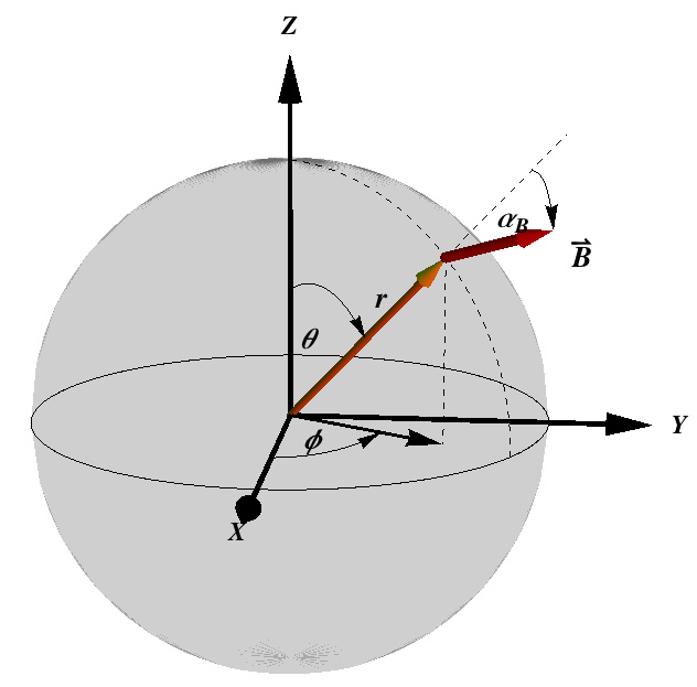
Figure 1: Illustration of the star, permeated by a dipolar magnetic field with identification of the Cartesian coordinates ($X,Y,Z$), and the spherical coordinates ($r,\theta,\phi$). Shown is also the vector magnetic field, $\vec{B}$, at a co-latitude $\theta$ and the angle $\alpha_{B}$ between the radial direction and the direction of the local magnetic field.

2.2 Pulsation model

The pulsation model is based on that adopted for the MAPPA code (MAgnetic Perturbations to Pulsations in Ap stars) (Cunha, 2006). In that model two regions are considered, namely, the interior of the star where the magnetic pressure is neglected and the outer layers, named by the author the magnetic boundary layer, where the magnetic pressure is comparable or larger than the gas pressure. In the interior, the standard oscillation model is used to describe the p-modes. In the Magnetic boundary layer, with a characteristic depth of only a few % of the radius, the author considers the direct effect of the magnetic field on the pulsations, and describes them by the following system of magnetohydrodynamic equations:

$$\dfrac{\partial\vec{B}}{\partial t}=\triangledown\times(\vec{v}\times\vec{B}),$$ (1)

$$\dfrac{D\rho}{Dt}+\rho\triangledown\cdot\vec{v}=0,$$ (2)

$$\rho\dfrac{D\vec{v}}{Dt}=-\triangledown p+\vec{j}\times\vec{B}+\rho\vec{g},$$ (3)

$$\dfrac{Dp}{Dt}=\frac{\gamma p}{\rho}\dfrac{D\rho}{Dt},$$ (4)

where the current density is $\vec{j}=1/\mu_{0}\,\nabla\times\vec{B}$, $\mu_{0}$ is the permeability in the vacuum, $\rho$ is the density of the gas, $p$ is the pressure, $\vec{g}$ is the gravitational field, $\vec{\xi}$ is the displacement vector and $\vec{v}=\partial\vec{\xi}/\partial t$ is the velocity. The system represents adiabatic motions, in the limit of perfect conductivity and is solved for small perturbations to the equilibrium structure and under the Cowling approximation.

Since the magnetic boundary layer is thin and the magnetic field varies on large scales only, the equations in this region of the star are solved by performing a plane-parallel approximation and assuming a local constant magnetic field, at each latitude. Consequently, at each latitude a local-coordinate system $(x,y,z)$ is defined with the $z$ component pointing outwards of the star, and such that the magnetic field is zero in the $y$ direction. The local magnetic field at a given co-latitude $\theta$, is then given by,

$$\vec{B}=\left(\frac{B_{p}}{2}\sin(\theta),0,B_{p}\cos(\theta)\right),$$ (5)

where $B_{p}$ is assumed to be constant, which is a good approximation given that the layer is thin.

Furthermore, since the system is solved under a linear approximation it does not inform about the amplitude of the displacement.

In what follows we will consider only solutions corresponding to the azimuthal order $m=0$, thus, the solution for the displacement at each latitude, in the local coordinate system, will be written as $\vec{\xi}=(\xi_{x},0,\xi_{z})$. Moreover, a second coordinate system will be used in the local approximation, namely, one that has axes parallel and perpendicular to the magnetic field. The latter coordinate system is obtained from the first through a rotation of $\alpha_{B}$ around the $y$ axis. We denote it by $(u_{\parallel},y,u_{\perp})$. In the second coordinate system the solutions are written in the form $\vec{\xi}=(\xi_{\parallel},0,\xi_{\bot})$.

In order to understand the solutions given by the MAPPA code (Cunha, 2006) we need to consider separately the two different regions mentioned before, namely the magnetic boundary layer of the star, and the interior. In the latter, dominated by the pressure of the gas, we find two decoupled solutions, an acoustic wave, that is displacing the gas in the radial direction, and a transverse Alfvén wave that is displacing the gas in a local horizontal direction (Cunha & Gough, 2000; Dziembowski & Goode, 1996). Moreover, in the magnetic boundary layer the solutions can be best understood by further dividing this layer into two different regions (Cunha, 2007), namely, the region where the pressure of the gas is of the same order of magnitude as the magnetic pressure and the outermost layers, where the magnetic pressure dominates. In the former, we have magnetoacoustic waves, while in the latter the waves decouple once again in the form of acoustic waves that are displacing the gas in the direction parallel of the magnetic field, and of compressional Alfvén waves, that are displacing the gas in the direction perpendicular to the magnetic field (Sousa & Cunha, 2008b).

2.3 Decoupling of the waves

The system of equation (1)-(4) is solved up to a normalizing constant by applying adequate boundary conditions. At the surface the magnetic field is matched continuously onto a vacuum field. The remaining boundary conditions are obtained by matching the numerical solutions to approximate analytical solutions in the regions where the magnetic and acoustic waves are decoupled, as described below.

In the interior of the star the acoustic component corresponds to the solution obtained when $\vec{B}=0$ and the magnetic component is assumed to be a wave that dissipates inside the star. Then, there the numerical solution for the magnetic component is matched onto an analytical asymptotic solution for an Alfvén wave propagating towards the interior of the star (see Cunha & Gough (2000) for details).

The final boundary condition consists in matching the numerical solution for the parallel component of the displacement to its analytical counterpart in the isothermal atmosphere. In the isothermal atmosphere the analytical solutions are those derived in the work of Sousa & Cunha (2011). There the magnetoacoustic waves are already decoupled into a (slow) acoustic wave and a (fast) compressional Alfvén wave that move in the directions parallel and perpendicular to the magnetic field, respectively, and have the form,

$$\xi_{\parallel}=\frac{|A_{s}|}{p^{1/2}}\exp{i(\pm k_{\parallel}\eta+\omega t+\phi_{s})},$$ (6)

$$\xi_{\bot}=|A_{f}|J_{0}(2\sqrt{\chi\rho})\exp{i(\omega t+\phi_{f})},$$ (7)

where $\omega$ is the angular oscillation frequency, $A_{s}$,$\phi_{s}$,$A_{f}$,$\phi_{f}$ are the amplitudes (A) and phases ($\phi$) of the acoustic and magnetic waves respectively, at the bottom of the isothermal atmosphere, that depend on the latitude, $J_{0}$ is the Bessel function and $\chi$ is a constant $\chi=H^{2}\omega^{2}\mu_{0}/B_{p}^{2}$. Moreover, the parallel component of the wavenumber is defined by:

$$k_{\parallel}=\sqrt{\frac{\omega^{2}\rho}{\gamma p\cos^{2}\alpha_{B}}-\frac{1}{4H^{2}}},$$ (8)

where $\gamma$ is the fist adiabatic exponent. $k_{\parallel}$ can be real or imaginary. In the former case the parallel component of the solution (acoustic wave) is oscillatory, while in the latter case it is exponential.

Inspecting the parallel component of the wave number $k_{\parallel}$, we can see that it depends on latitude through the angle $\alpha_{B}$. Therefore, even when the frequency of the oscillation is below the acoustic cut-off frequency for a non-magnetic star, in the presence of a magnetic field $k_{\parallel}$ will become real and the solutions will become oscillatory when the co-latitude is larger than a given critical value. The critical frequency,

$$\omega_{c}=\sqrt{\frac{\gamma p\cos^{2}\alpha_{B}}{4H^{2}\rho}},$$ (9)

defines the co-latitude at which the parallel component of the solution changes its behavior from exponential to oscillatory in the presence of the magnetic field. We shall call that co-latitude the critical angle, $\alpha_{cr}$

For a dipolar magnetic field, the critical frequency has its maximum value at the magnetic pole, corresponding to the the critical frequency in the absence of a magnetic field, (i.e. to the acoustic cut-off frequency). But it decreases as the magnetic equator is approached. As a consequence, even if the oscillation frequency is below the acoustic cut-off frequency, it will always be above the local critical frequency for co-latitudes larger than a critical value and, thus, there will always going to be wave energy losses in the equatorial zone when the magnetic field is considered.

2.4 Displacement solutions

Due to the structure of the magnetic field, at each latitude the distortion of the oscillation is different. In particular, the magnitude and direction of the magnetic field is different at different latitudes, affecting differently both the amplitude and characteristic scale of the displacement. To illustrate this, we discuss below a particular case, at two different latitudes.

The displacement as a function of the radius at two different latitudes is shown for a cyclic frequency ($f=\omega/2\pi$) of $1.7$ mHz and a magnetic field, $B_{p}$, of $2$ kG, in Figs. 2 and 3. On the left panels we show the components of the solution in the innermost part of the magnetic boundary layer, using the local coordinate system (x,y,z), and on the right panels the local parallel and perpendicular components of the solution in the outermost part of the magnetic boundary layer, using the coordinate system $(u_{\parallel},y,u_{\perp})$.

In Fig. 2 the displacement is shown for a co-latitude of $37^{\circ}$. At this latitude the frequency is below the critical frequency and, thus, in the isothermal atmosphere, marked by the yellow-shaded region on the right panels, the acoustic wave (component of the displacement parallel to the magnetic field) shows a standing behavior as does the compressional Alfvén wave (perpendicular component), which shows, in addition, a constant amplitude in that part of the atmosphere, as expected from eq. (7).

In the inner layers shown on the left panels, the acoustic wave (vertical component $\xi_{z}$ in these layers), also presents an almost standing behavior while the Alfvén wave (the horizontal component $\xi_{x}$) has a clear running behavior, dissipating towards the interior of the star as expected from the boundary conditions.

Figure 3 illustrates a case of a co-latitude of $87^{\circ}$. As expected, closer to the equator, where the frequency of the wave is larger than the critical frequency, the acoustic wave will, instead, have a running behavior in the atmosphere. As a consequence, at this co-latitude the exponential growth of the wave amplitude is larger than at the co-latitude of $37^{\circ}$. Because the energy carried by the acoustic wave is conserved, the wave amplitude thus increases as the inverse of the root square of the density (or, equivalently in these layers, of the root square of the pressure- cf eq. (6)). We note, for comparison, that for the co-latitude of $37^{\circ}$, the exponential term in eq. (6) partially compensates the exponential increase associated with the decrease of the pressure, leading to a smaller increasing rate of the amplitude, consistent with a decrease in the energy content of the acoustic wave.

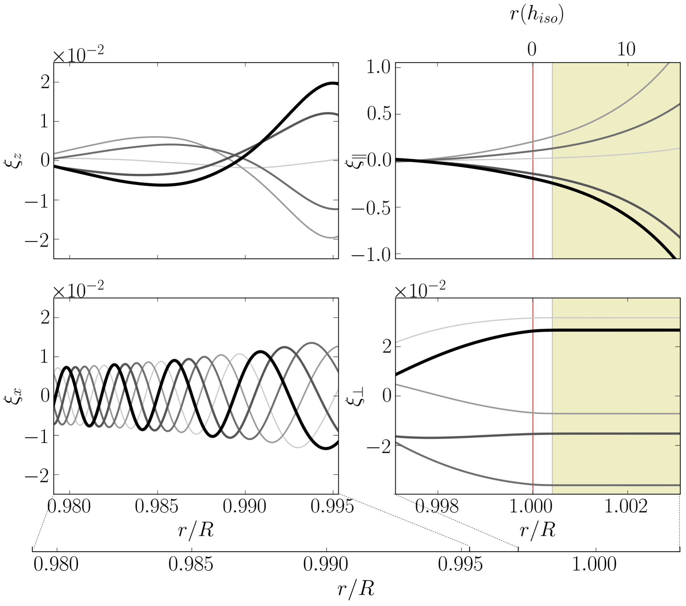
Figure 2: Dimensionless displacement $\vec{\xi}$ at the co-latitude of $37^{\circ}$, as a function of the normalized radius (bottom x axis) in the outer $2\%$ of the stellar model, for a frequency $1.7$ mHz with a magnetic field of $2$ kG. The left panels show the components of the displacement in the local vertical (top) and local horizontal (bottom) directions. The right panels show the displacement in the direction parallel to the magnetic field (top), and perpendicular to the magnetic field (bottom). The different curves represent different times, the yellow shadow marks the isothermal atmosphere, and the red vertical line represents the bottom of the photosphere of the star. The top x axis indicates the atmospheric height measured from the bottom of the photosphere in units of the (constant) pressure scale height of the isothermal atmosphere.

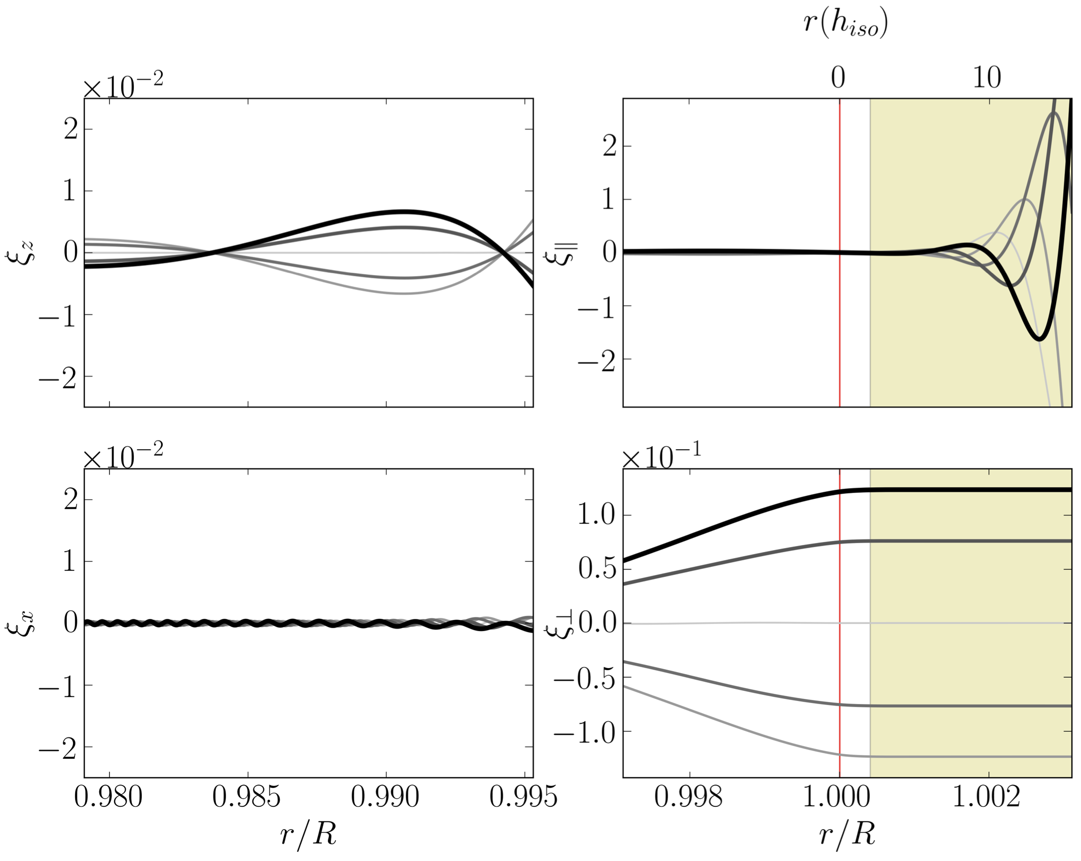
Figure 3: The same as in figure 2 but for a co-latitude of $87^{\circ}$.

2.5 Radial velocities

To obtain the radial velocity as a function of the radius in the outer layers of a roAp star we need to integrate the velocity field at each specific radius over the area of interest, which may be the full visible disc, or a sub-section of it, when the elements contributing to the radial velocity measurement are concentrated in a particular region only. We compute the integrated velocity field, considering a liner limb-darkening law, using the expression (Dziembowski, 1977),

$$V_{int}=\int\limits_{\varphi^{\prime}_{i}}^{\varphi^{\prime}_{f}}\int\limits_{\theta^{\prime}_{i}}^{\theta^{\prime}_{f}}\left[v_{r}X_{r}+v_{\theta}X_{\theta}\right]\times C_{n}^{-1}(1-a(1-\cos{\theta^{\prime}}))\cos{\theta^{\prime}}\sin{\theta^{\prime}}d\theta^{\prime}d\varphi^{\prime},$$ (10)

where $(r,\theta,\phi)$ is the spherical coordinate system, described in Fig. 1, $(r,\theta^{\prime},\phi^{\prime})$ is a spherical coordinate system with the polar axis, here named $Z^{\prime}$, aligned with the direction of the observer, $a$ is the limb-darkening coefficient, for which we adopt a value of 0.46 (Claret & Hauschildt, 2003), and $C_{n}$ is a normalization constant from the integration of the limb-darkening in the visible disc. $\varphi^{\prime}_{i}$, $\varphi^{\prime}_{f}$ and $\theta^{\prime}_{i}$, $\theta^{\prime}_{f}$, are the integration limits, that represent a given area of the visible disk. $X_{r}$ and $X_{\theta}$ are the projections of the unit vector along the radial direction $\widehat{r}$ and along the polar direction, $\widehat{\theta}$ onto the direction of the observer $\widehat{z}^{\prime}$, respectively. Moreover, $v_{r}$ and $v_{\theta}$ are the velocity components derived from the displacement, $\vec{v}=\dfrac{d}{dt}\delta\vec{r}$, where,

$$\delta\vec{r}=\left(\xi_{r}(r,\theta)Y_{l}^{0}\,\,\widehat{r}+\xi_{\theta}(r,\theta)Y_{l}^{0}\,\,\widehat{\theta}\right)\emph{e}^{\textit{i}\omega t}.$$ (11)

Here $\xi_{r}$ and $\xi_{\theta}$ are obtained by combining the local solutions $\xi_{z}$ and $\xi_{x}$, respectively, at each latitude. Their $\theta$ dependence is a consequence of the presence of the magnetic field which, as discussed before, influences the eigenfunction differently at different latitudes distorting the eigenfunctions from the pure spherical harmonic solutions obtained in the non-magnetic case. Moreover, since the system loses energy both from the running magnetic waves at the bottom of the magnetic boundary layer and from the acoustic running waves in the atmosphere, the eigenfrequencies and eigenfunctions are complex.

When considering the integration only in a certain region of the disk, corresponding to a chemical overabundance spot, the spot can be studied from different viewing angles, as illustrated in Fig. 4. We can, thus, study the changes in the radial velocity associated to a spot throughout the rotation of the star.

We also computed the integral for the radial velocity considering, instead, the limb-darkening and line-weighting proposed by (Landstreet & Mathys, 2000). However, using their main values for the coefficients proposed, we did not find a significant difference when comparing to the results obtained with eq (10).

To facilitate the physical interpretation of the radial velocity $V_{int}$, the code allows us to separate the contributions to $V_{int}$ of the different components of the velocity perturbation. This is done by performing an integral that is in all equal to that defined in Eq. (10), except that the total velocity projected in the direction of the observer that enters that integral is substituted by the projection of a single component of the velocity. This facilitates the physical interpretation because in the outer atmospheric layers the acoustic waves correspond to displacements parallel to the magnetic field while the magnetic waves correspond to displacements perpendicular to the magnetic field. When the velocity field component aligned with the magnetic field alone is considered in that integral, we denominate the result of that integral $V_{\parallel}$. Similarly, when the integral is based on the velocity field component perpendicular to the magnetic field alone, we denominate the result of the integral by $V_{\perp}$. Moreover, we compute similar integrals considering the radial and polar components of the velocity denominating the results by $V_{r}$ and $V_{\theta}$, respectively.

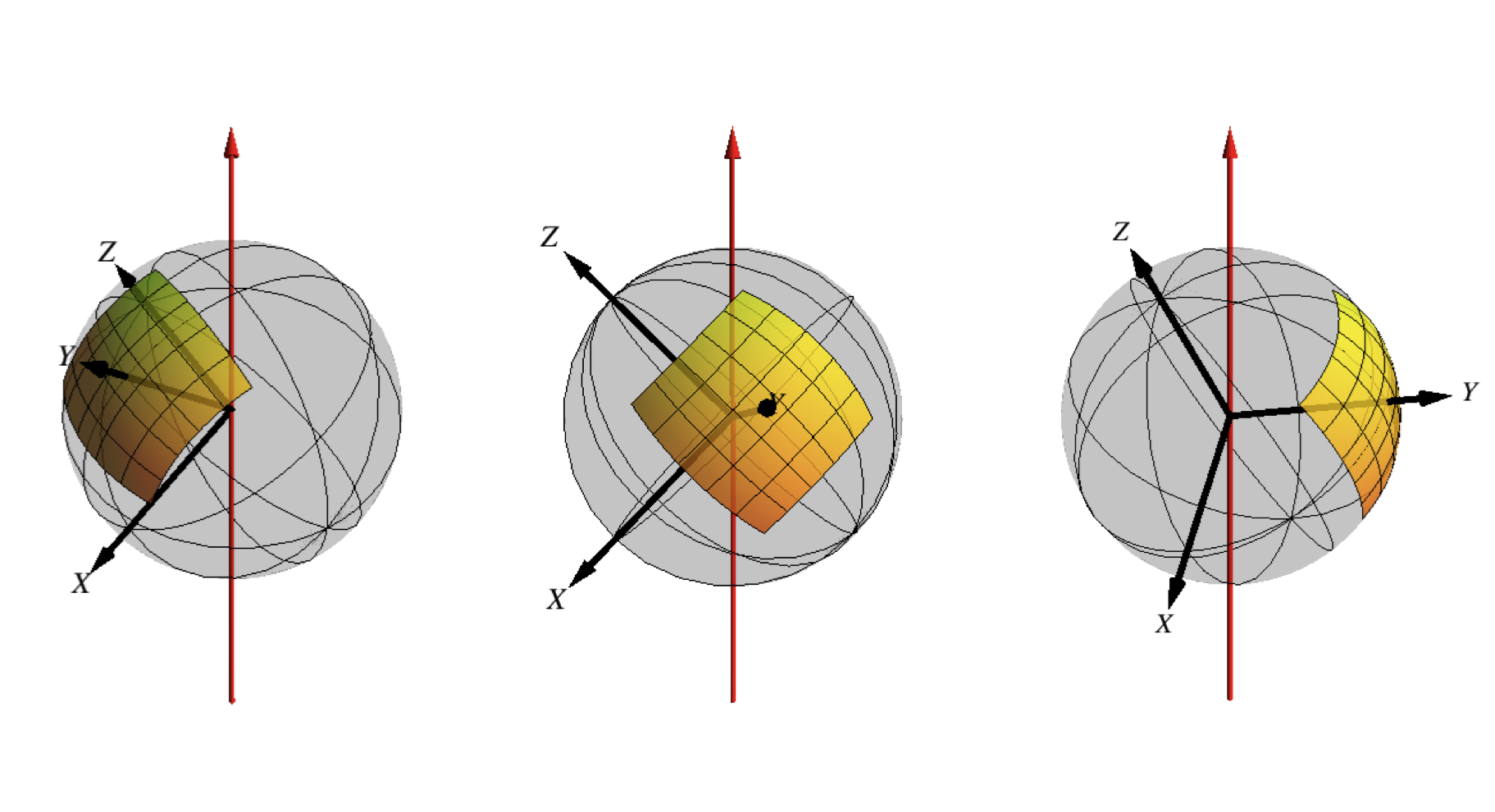
Figure 4: Representation of a spot in the code to calculate the radial velocity, considering the star at different rotational phases.

In summary, the code allows us to compute the radial velocity associated to the stellar pulsations, either for the full visible disk or for part of it. Being able to define any area in the surface of the sphere, that can represent a spot or a belt of elements in the atmosphere of the star, and redefining the limits of integration, $\varphi^{\prime}_{i}$, $\varphi^{\prime}_{f}$, $\theta^{\prime}_{i}$ and $\theta^{\prime}_{f}$, so that these always remain in the visible disk, the code makes it possible to study the pulsations for different positions of the observer, for a single spot or the full visible disk. In addition, it allows us to study the contributions to the radial velocity of the different components of the velocity field.

3 Results

To analyze different possible solutions, we fix the magnetic field in $2$ kG and explore 3 different pulsation frequencies. For the first three cases we consider that the observer is pole-on and that the mode degree is $l=1$. In addition, we analyze three cases in which the observer’s position is equator-on and the mode degree is $l=0$. In doing so, in particular by fixing the frequencies, we intentionally ignore the difference in frequency that would result from solving the eigenvalue problem for modes of different degrees. We note that we did not consider an odd degree mode for the equator-on view because of the strong cancellation effect that would be present when performing the disk integration. These cases correspond to the first 6 entries in Table 2.

Table 2: Properties and parameters of the cases explored in this work. The columns are: frequency, $f$; polar magnetic field, $B_{p}$; observer’s view; integration area, that can be of the full visible disk (F. V. D.), or of a belt in the equatorial zone (E. Z.); and the critical angle, $\alpha_{cr}$.

	$f$	$B_{p}$	Obs.	l	Int.	$\alpha_{cr}$
	mHz	kG	from		area
Case 1	1.7	2.0	pole	1	F. V. D.	$50^{\circ}$
Case 2	2.2	2.0	pole	1	F. V. D.	$33^{\circ}$
Case 3	2.7	2.0	pole	1	F. V. D.	$0^{\circ}$
Case 4	1.7	2.0	equator	0	F. V. D.	$50^{\circ}$
Case 5	2.2	2.0	equator	0	F. V. D.	$33^{\circ}$
Case 6	2.7	2.0	equator	0	F. V. D.	$0^{\circ}$
Case 7	2.7	2.0	pole	0	E. Z.	$0^{\circ}$

For a $2$ kG magnetic field, the magnetoacoustic region in our stellar model is placed fully in the interior of the star. This is illustrated in Fig. 5 where the gas and magnetic pressures are compared. This means that in the atmospheric region the acoustic and magnetic waves are completely decoupled and, as noted in the section 2, the acoustic waves move in the direction of the local magnetic field, and the magnetic waves move perpendicularly to it.

In addition, we consider a case in which an apparent node in the isothermal atmosphere can be seen. This corresponds to the last entry in Table 2.

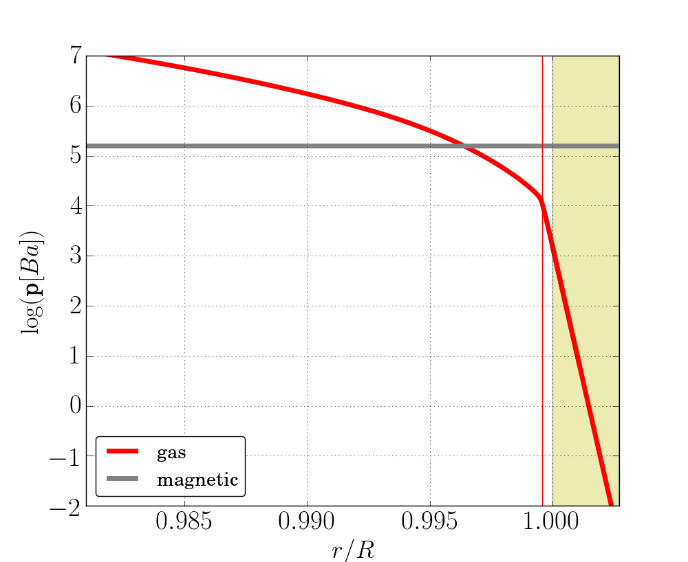
Figure 5: Comparison between the gas pressure (thick red line) and the magnetic pressure (grey line) in the outer 2% of the star for a magnetic field of 2 kG. The thin vertical red line marks the bottom of the photosphere.

To compare the amplitude, $A_{r}$, and phase, $\phi_{r}$, variations of the theoretical radial velocity with those derived from observations (e.g. Ryabchikova et al. (2007a)), we match the numerical solutions in the atmosphere to a function of the type,

$$V_{int}=A_{r}\cos(\omega t+\phi_{r}).$$ (12)

3.1 Case 1

The first case we discuss, is one in which the phase is found to be nearly constant. To find a solution with a constant phase it is necessary to choose a frequency well below the acoustic cut-off. Here we take a frequency of $1.7$ mHz. As we mentioned earlier, we fix the magnetic field at $B_{p}=2$ kG, and consider a mode of degree $l=1$ with an observer pole-on. At this particular frequency, the acoustic waves change from having a standing character to having a running character at a critical angle $\alpha_{cr}=50^{\circ}$ (see Table 2), meaning that for co-latitudes larger than this angle the local critical frequency is smaller than $1.7$ mHz. The radial velocity is shown in the left panel of Fig. 6. The contributions of the components of the velocity parallel and perpendicular to the magnetic field to the integral that defines the radial velocity (eq. (10)) are presented in the top- and bottom-right panels, respectively. In each panel the vertical red line indicates the bottom of the photosphere of the star and the shaded-yellow area represents the isothermal atmosphere. The same notation is used for all other cases.

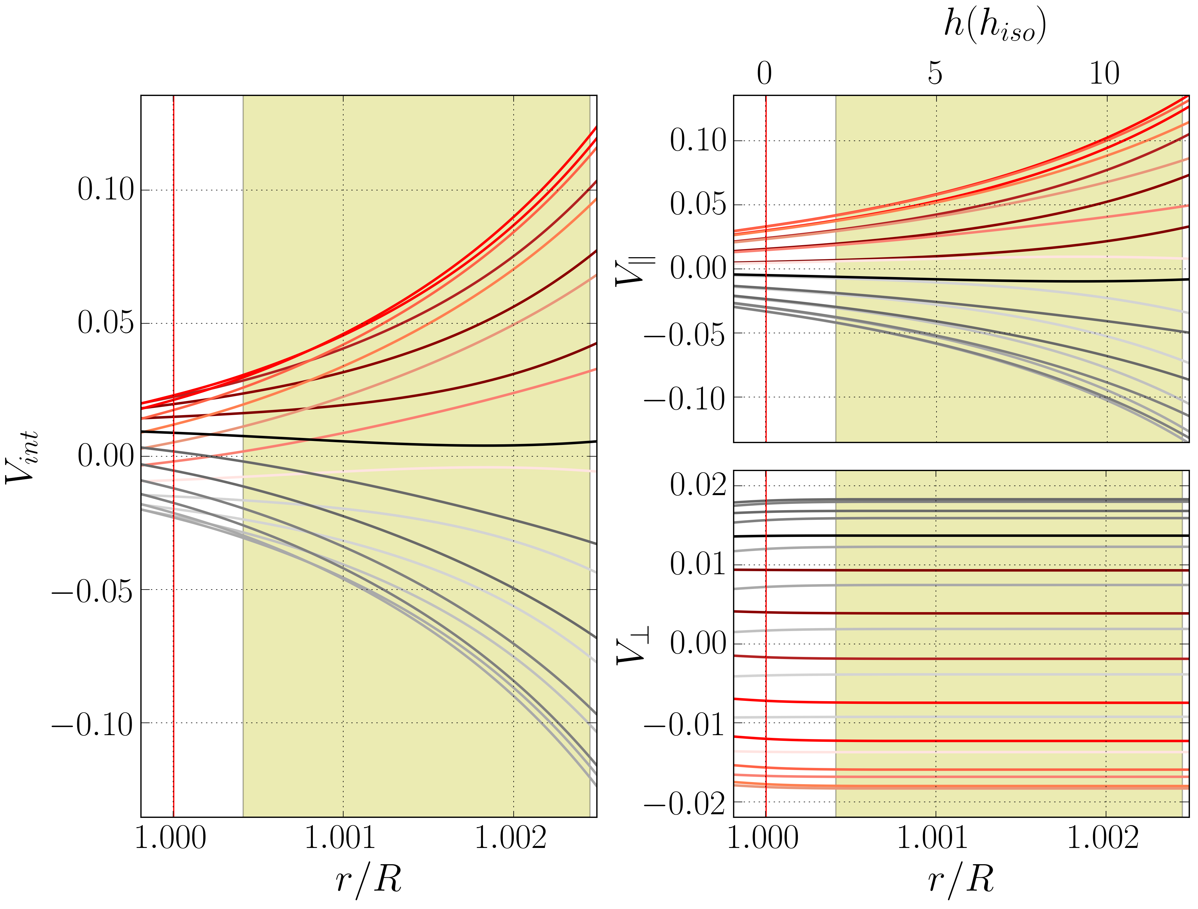
Figure 6: Dimensionless and normalized radial velocity. This case is for integration over the visible disc, a magnetic field of $2$ kG, a mode of frequency $1.7$ mHz and degree $l=1$, and an observer pole-on. Shown in the left panel is the radial velocity as a function of the radius, at different times within the oscillatory period represented by curves of different colors. The upper right panel shows the contribution to the radial velocity of the velocity component parallel to the magnetic field. The bottom right panel shows the contribution to the radial velocity of the velocity component perpendicular to the magnetic field. The labels on the top horizontal axes show the height measured from the bottom of the photosphere in units of the (constant) pressure scale height of the isothermal atmosphere. The red vertical line represents the bottom of the photosphere and the yellow shadow region represents the isothermal atmosphere.

Looking at the contribution of the parallel and perpendicular velocity components in the atmosphere of the star, we can verify that the acoustic and magnetic waves are already decoupled, since, as predicted analytically by eqs. (6)-(7), we see an exponential behavior for the parallel component, and a constant behavior for the perpendicular component. Their contribution to the radial velocity integral is of similar magnitude, although the acoustic waves become progressively dominant with increasing atmospheric height.

The amplitude and phase of the radial velocity for this case are shown in Fig. 7. The left panel shows the amplitude variation during one period of the oscillation at different heights in the atmosphere. We recall that the amplitude of the oscillation is only known up to a normalizing constant. In this particular plot (and in similar plots for the other cases) we chose that constant in such a way as to make the oscillation visible to the reader. The right hand-side panels show the amplitude (top panel) and phase (bottom panel) of the radial velocity as a function of the height in the atmosphere.

As we can see from the top-right panel, the total amplitude (i.e., the amplitude derived from fitting the radial velocity - black line) follows the behavior of the parallel amplitude, derived from the fitting of $V_{\parallel}$ and related to the contribution of acoustic waves (red line). It is, however, always smaller than the parallel amplitude because of the contribution from the magnetic waves, whose amplitude is derived from the fitting of $V_{\perp}$ (gray line). In the bottom-right panel, we see that the total phase (black line) follows relatively closely the parallel (acoustic) phase (red line) in the outermost layers, but diverges from it in the lower atmospheric region due to the increasing impact of the perpendicular (magnetic) phase. Despite this, the phase variation across the whole atmosphere is small. The left panel of Fig. 7 gives us also an idea of the behavior of the phase. In the present case we can confirm the small variation of the phase with height, seen in the slight shift of the zeros to the right, as we move towards higher atmospheric layers.

This is a clear case in which the phase variation in the radial velocity results from the competition between the acoustic and magnetic components that enter the integral, rather than from an actual phase variation in either of them. The perpendicular phase is always constant, due to the standing nature of the magnetic waves, while the parallel phase, related with the acoustic component, is constant due to the pole-on view, that favours the area where the standing waves are located, and the low value of the frequency that guarantees that the standing acoustic waves occupy a larger area in the visible disk of the star than the acoustic running waves.

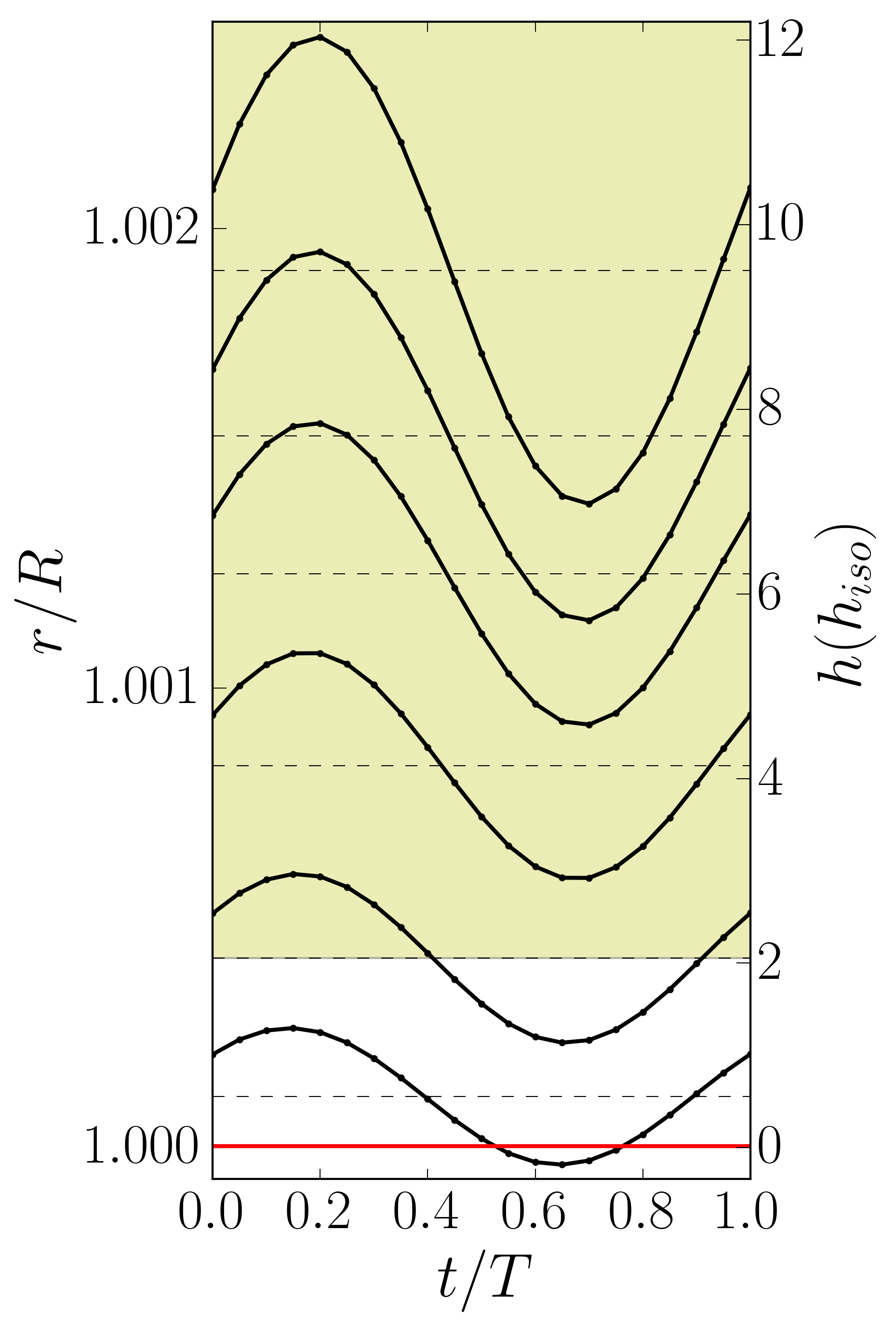
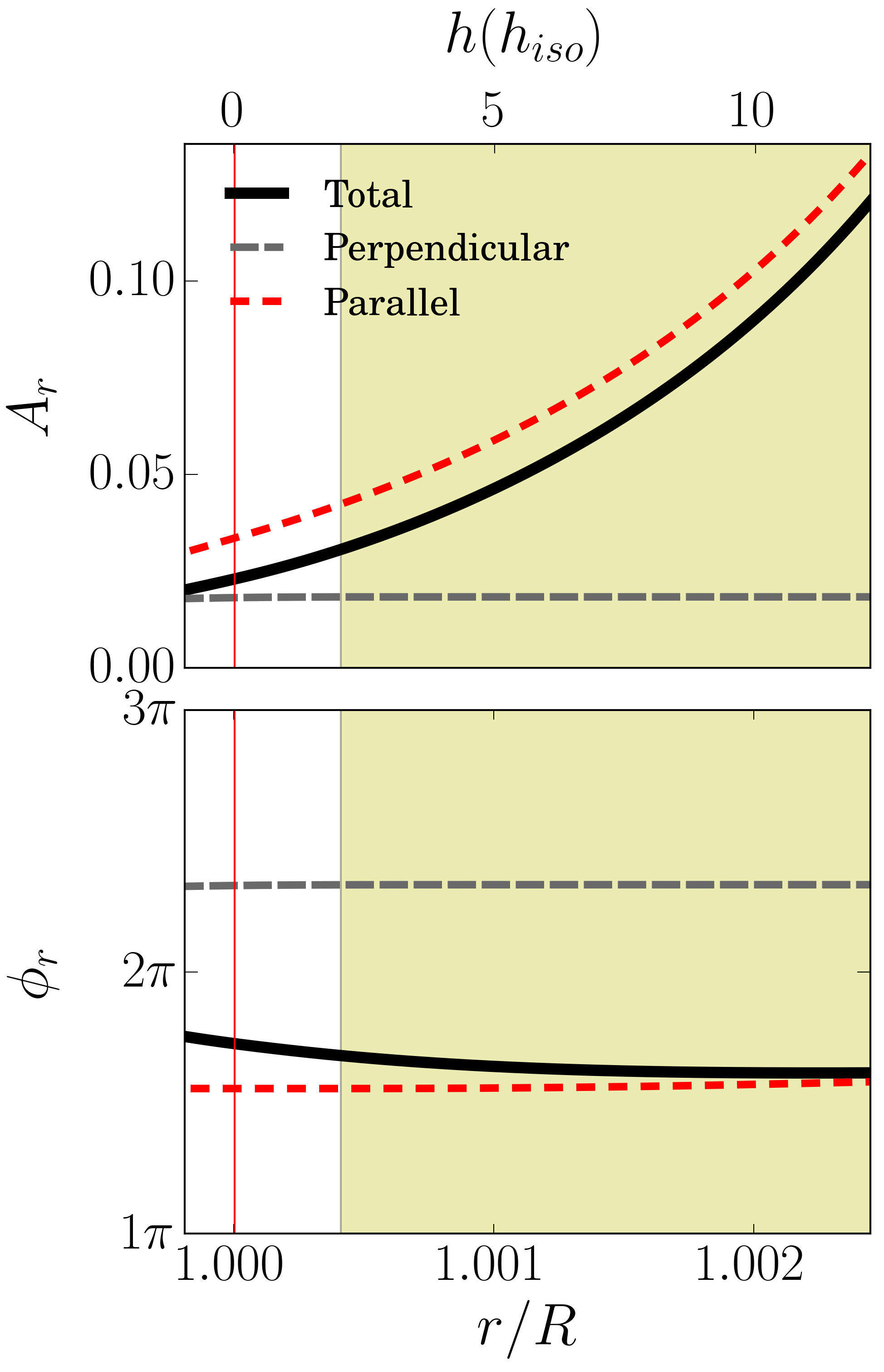
Figure 7: The left panel shows the amplitude of the radial velocity at different heights in the atmosphere, as a function of the fraction of time within an oscillation period T. The right panels show the amplitude (top) and the phase (bottom) of the radial velocity fitted to the function given by eq. (12). The radial velocity amplitude and phase are in black, the amplitude and phase derived from $V_{\parallel}$ in red, and the amplitude and phase derived from $V_{\perp}$ in grey. The horizontal red line on the left panel and the vertical red line on the right panel mark the bottom of the photosphere.

3.2 Case 2

For the second case we consider a frequency bellow the acoustic cut-of, but close to it. We have chosen a mode with a frequency of $2.2$ mHz, degree $l=1$, and an observer pole-on. The angle at which the critical frequency becomes smaller than $2.2$ mHz is $\alpha_{cr}=33^{\circ}$ (cf. Table 2). The radial velocity is shown on the left panel of Fig. 8, and the contributions to it from the components of the velocity parallel and perpendicular to the magnetic field are shown on the right panels, in the same way as for the previous case. We see, from the right panels, the exponential behavior of the acoustic wave’s contribution (top) in the atmosphere of the star, and the constant amplitude of the magnetic wave’s contribution (bottom), but this time the amplitudes of the two contributions differ more significantly in the high atmosphere. This is because in the present case the fraction of the visible disk covered with acoustic running waves is larger than in case 1. Since the amplitude of the displacement, hence also of the velocity, increases faster with height for running acoustic waves than for standing acoustic waves (as discussed in section 2.4), in the present case the acoustic contribution to the integral of the radial velocity becomes more dominant in the high atmosphere.

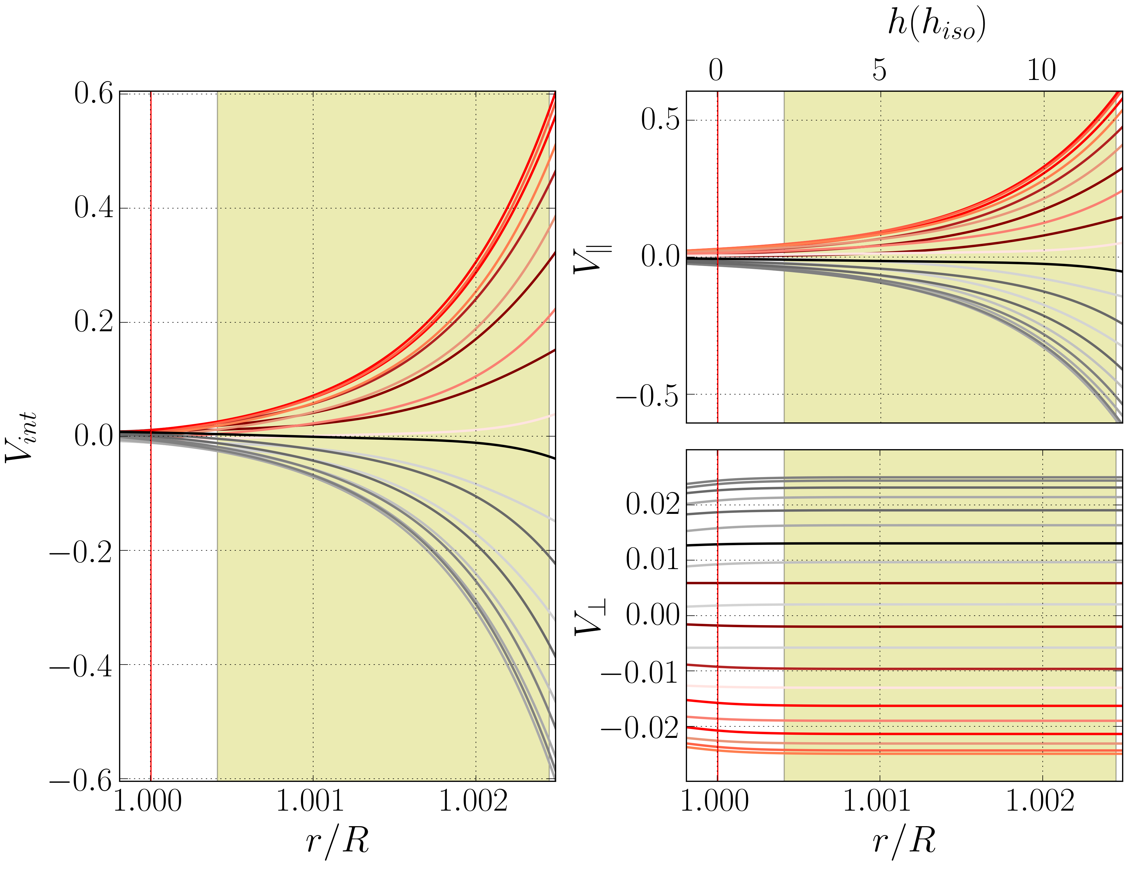
Figure 8: The same as Fig. 6 but for a mode of frequency $2.2$ mHz and degree $l=1$, a magnetic field of $2$ kG, and an observer pole-on.

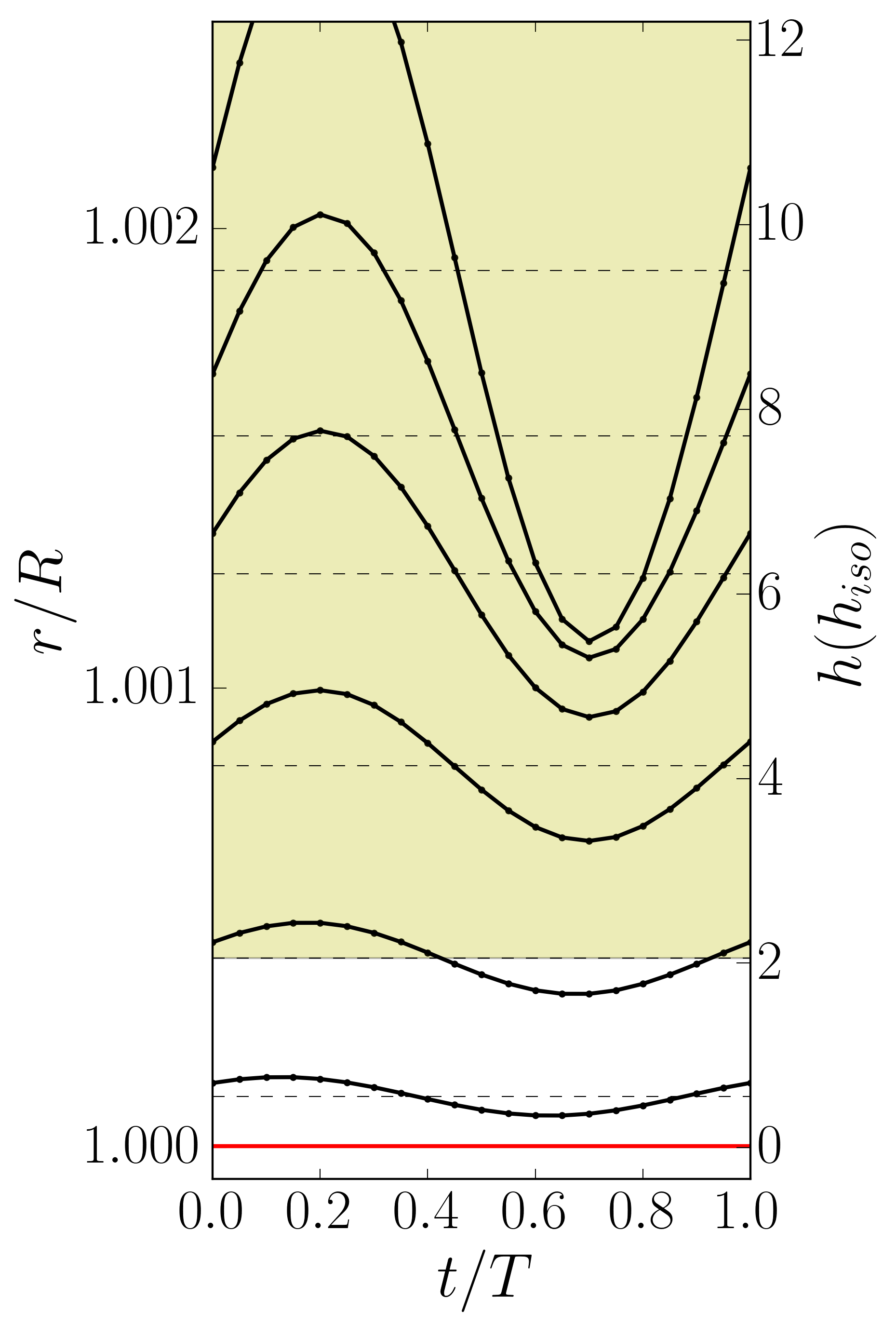
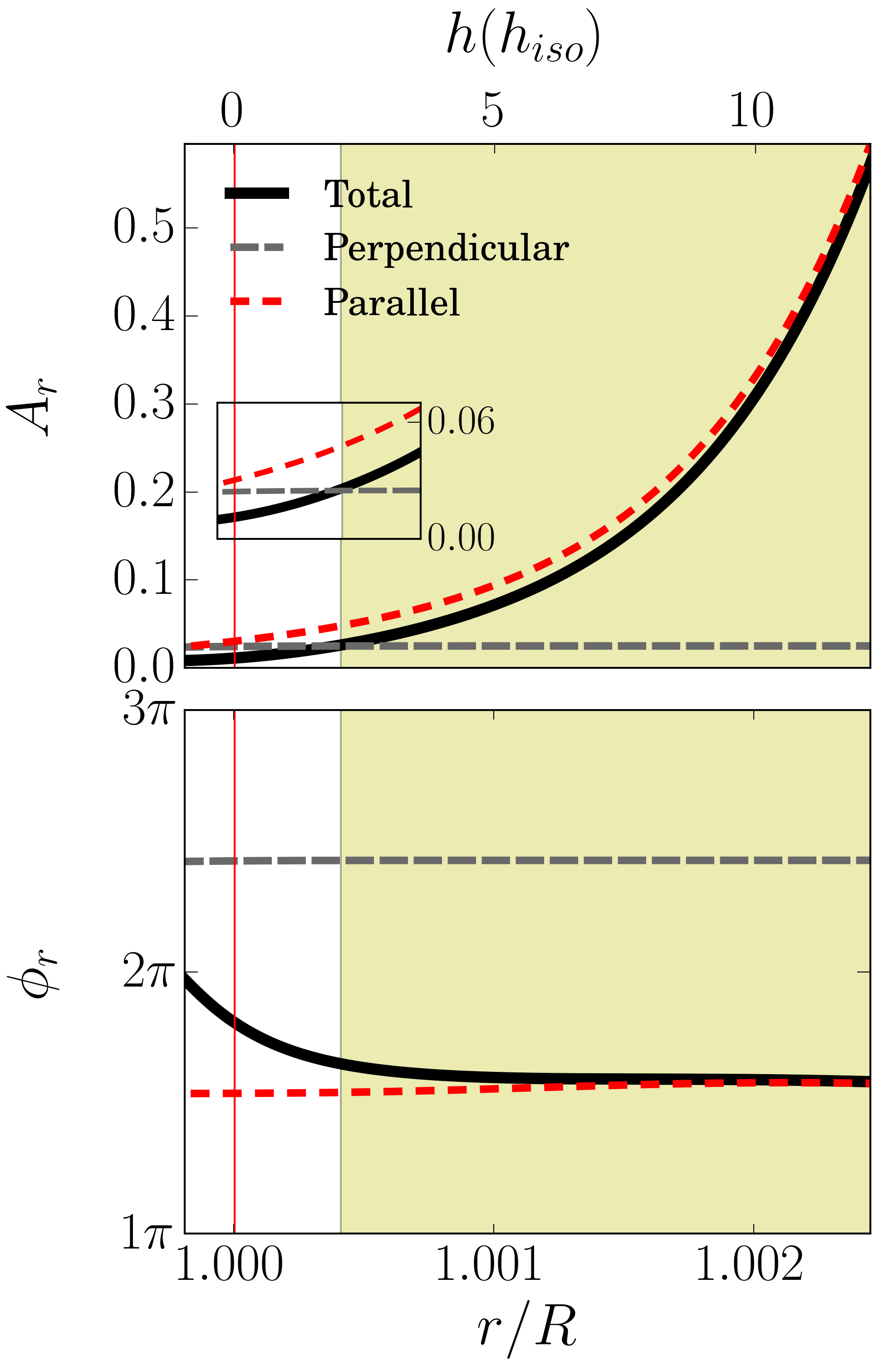
Figure 9: The same as Fig. 7 but for a mode of frequency $2.2$ mHz and degree $l=1$, a magnetic field of $2$ kG, and an observer pole-on. The close-up shows the behaviour of the amplitudes near the photosphere.

The amplitude and phase of the radial velocity are shown in Fig. 9, in the same manner as in the previous case. In the outermost layers the total amplitude (black line, top-right panel) follows the acoustic wave’s contribution (red line), but, when moving towards lower atmospheric layers the magnetic wave’s contribution (gray line) becomes increasingly important. This behavior can be seen also in the phase (bottom-right panel), as the total phase (black line) follows the phase from the acoustic wave’s contribution (red line) in the outer layers, but approaches the phase of the magnetic wave’s (gray line) contribution deeper in. Unlike in the previous case, here we can see a very small variation in the phase of the acoustic contribution (red line) which is due to the higher frequency of the mode considered that results in a more significant contribution of acoustic running waves to the integral of the parallel component. Nevertheless, the dominant phase variation in the radial velocity (black line) results from the competition between the contributions to the radial velocity integral of the parallel (acoustic) and perpendicular (magnetic) velocity components, as in the previous case.

Due to the small variations in the phase, a small shift in the zeros can also bee seen in Fig. 9, left panel, when looking at different atmospheric heights.

3.3 Case 3

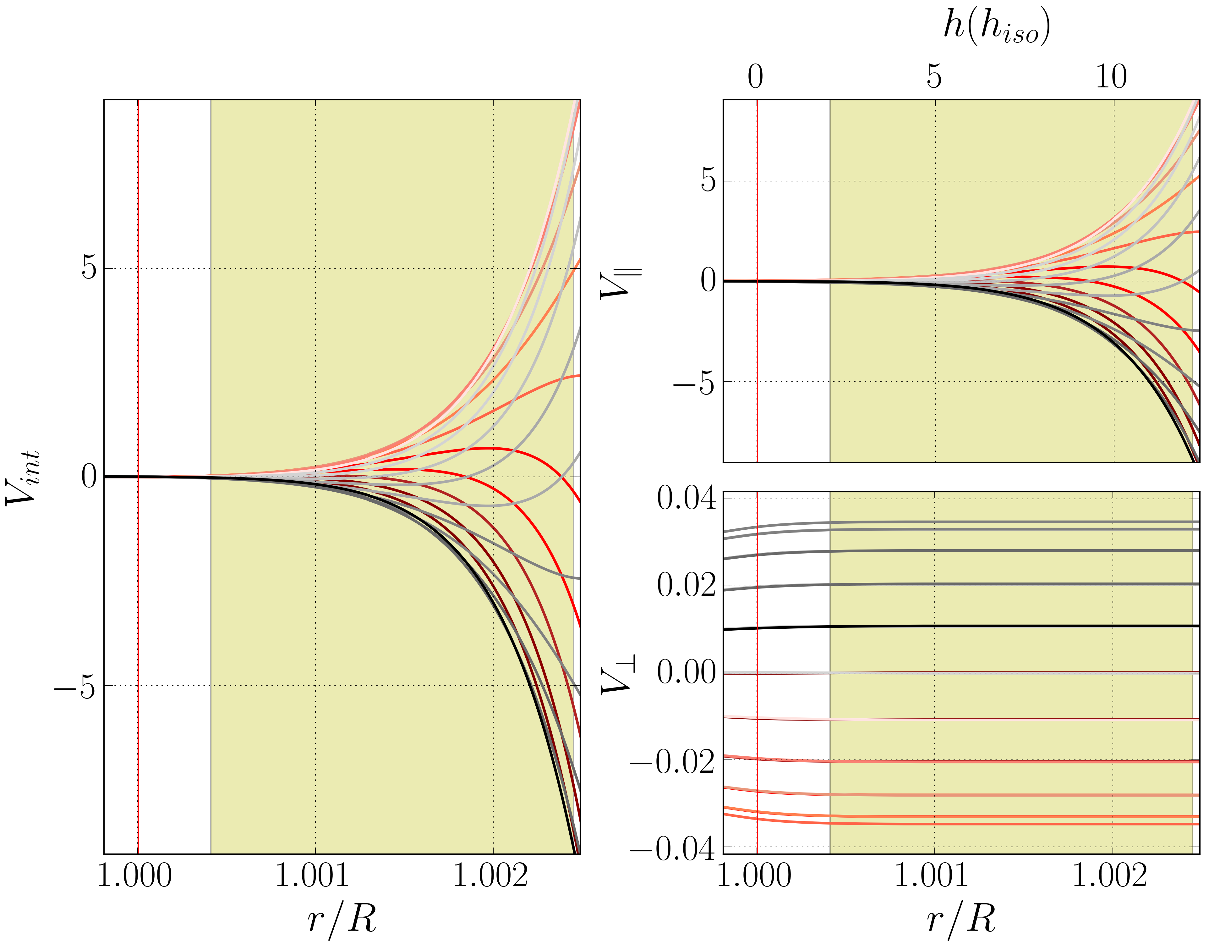
Figure 10: The same as Fig. 6 but for a mode of frequency $2.7$ mHz and degree $l=1$, a magnetic field of $2$ kG, and an observer pole-on.

The third case is one in which the phase is found to be more significantly variable. It is the last one we present with a pole-on observer and it concerns a mode with a frequency of 2.7 mHz, which is above the acoustic cut-off (cut-off frequency of the star in Table 1), and a degree of $l=1$ (Table 2). The radial velocity for this case is shown in Fig. 10, left panel. Since the mode frequency is above the acoustic cut-off, the acoustic running waves are present in the full visible disk. Due to the faster increase with height of acoustic running waves, the amplitudes of the acoustic wave’s contribution (top-right panel) and magnetic wave’s contribution (bottom-right panel) differ by 2 orders of magnitude in the outermost layers, leading to a total dominance of the acoustic waves in that part of the atmosphere.

The variations in the amplitude and phase for this case are shown in Fig. 11, top- and bottom-right panels, respectively. The variations in the total amplitude and the total phase (black lines) show the dominance of the acoustic wave’s contribution (red line) throughout the isothermal atmosphere. In that region we can see a significant variation of the parallel phase caused by the running acoustic waves. In the inner atmosphere, where the magnetic and acoustic contributions have the same order of magnitude, we can identify a crossing between the acoustic (red line) and the magnetic wave’s contributions (gray line). Together with the abrupt variation in the total phase (black line) this marks the transition between the dominance of the two types of waves in the radial velocity integral. Because they are out of phase, this crossing generates an apparent node in the inner atmosphere.

Looking at Fig. 11, left panel, the variation in the phase can be clearly seen, as a shift in the zeros of the oscillations when comparing different atmospheric heights.

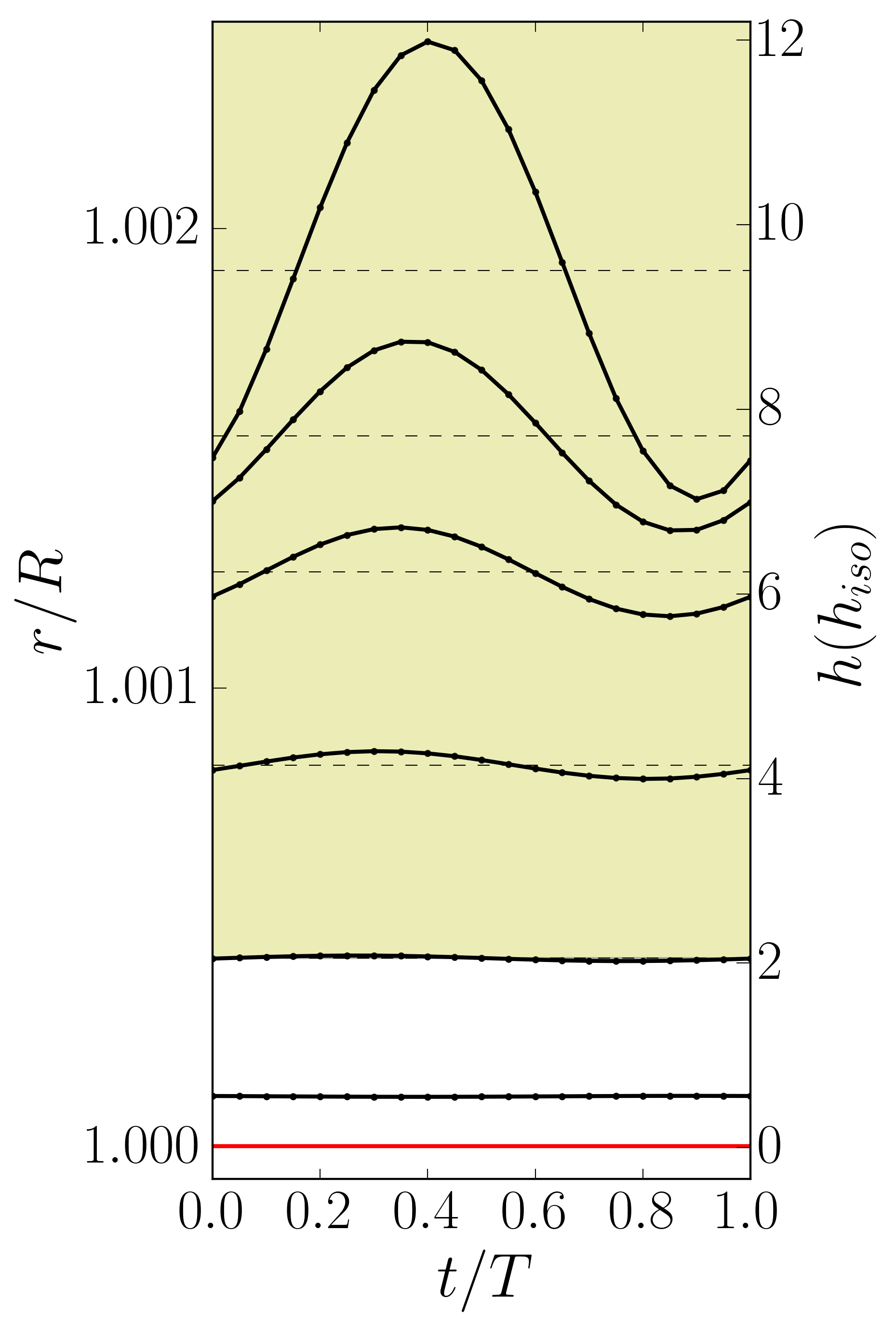
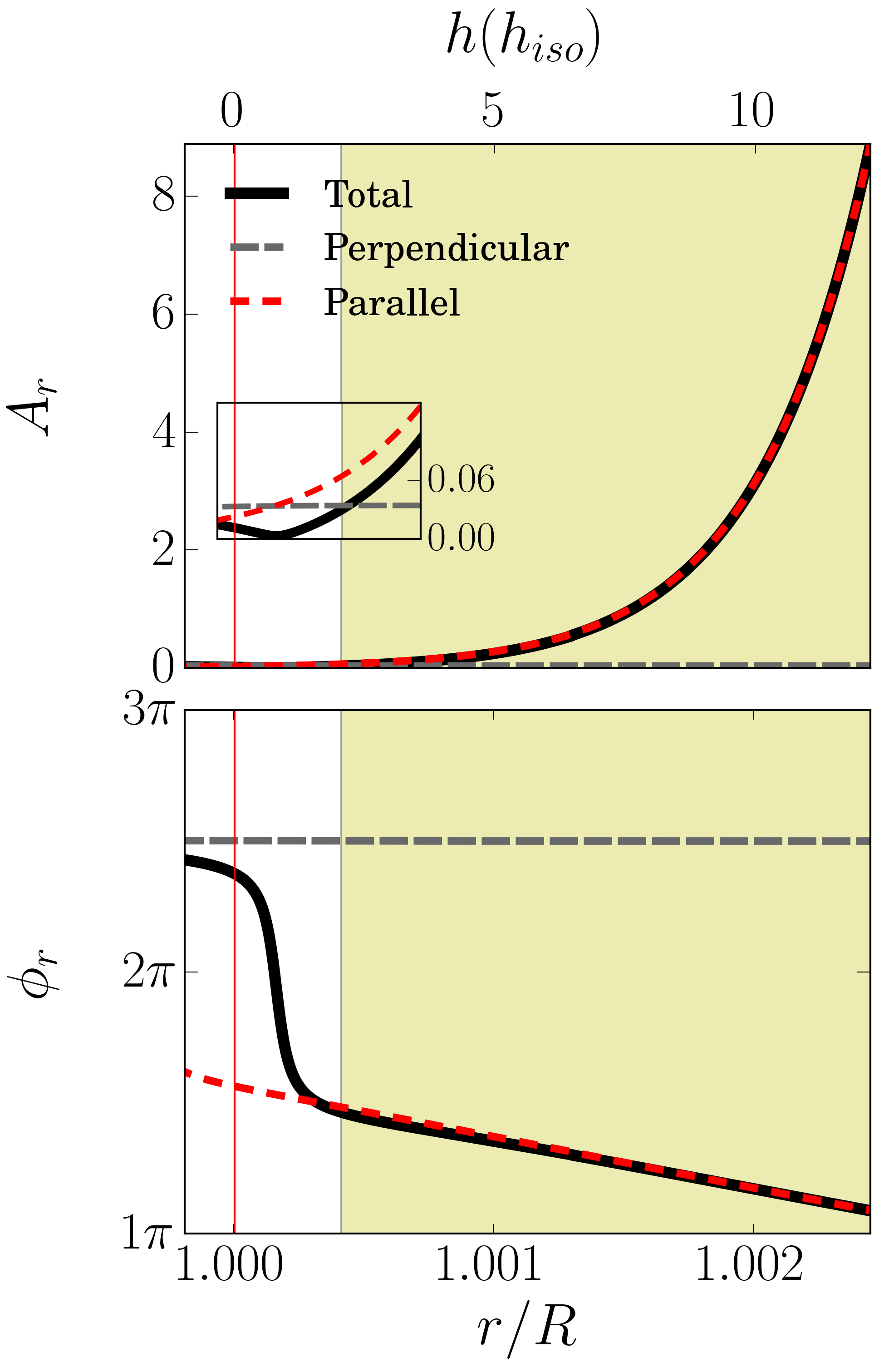
Figure 11: The same as figure 7 but for a mode of frequency $2.7$ mHz and degree $l=1$, a magnetic field of $2$ kG, and an observer pole-on. The close-up shows the behaviour of the amplitudes near the photosphere.

3.4 Case 4

The case 4 corresponds to an observer located equator-on and a mode with a frequency of $1.7$ mHz and degree $l=0$ (Table 2). The radial velocity for this case is shown in Fig. 12, left panel. The amplitudes of the acoustic and magnetic waves’ contributions (Fig. 12, right panels) are of the same order of magnitude in the lower part of the atmosphere, just as was found for case 1, although here the two contributions become comparable near the photosphere, as seen from Figure 13, right upper panel. But the main difference with respect to case 1 is the behavior of the phase.

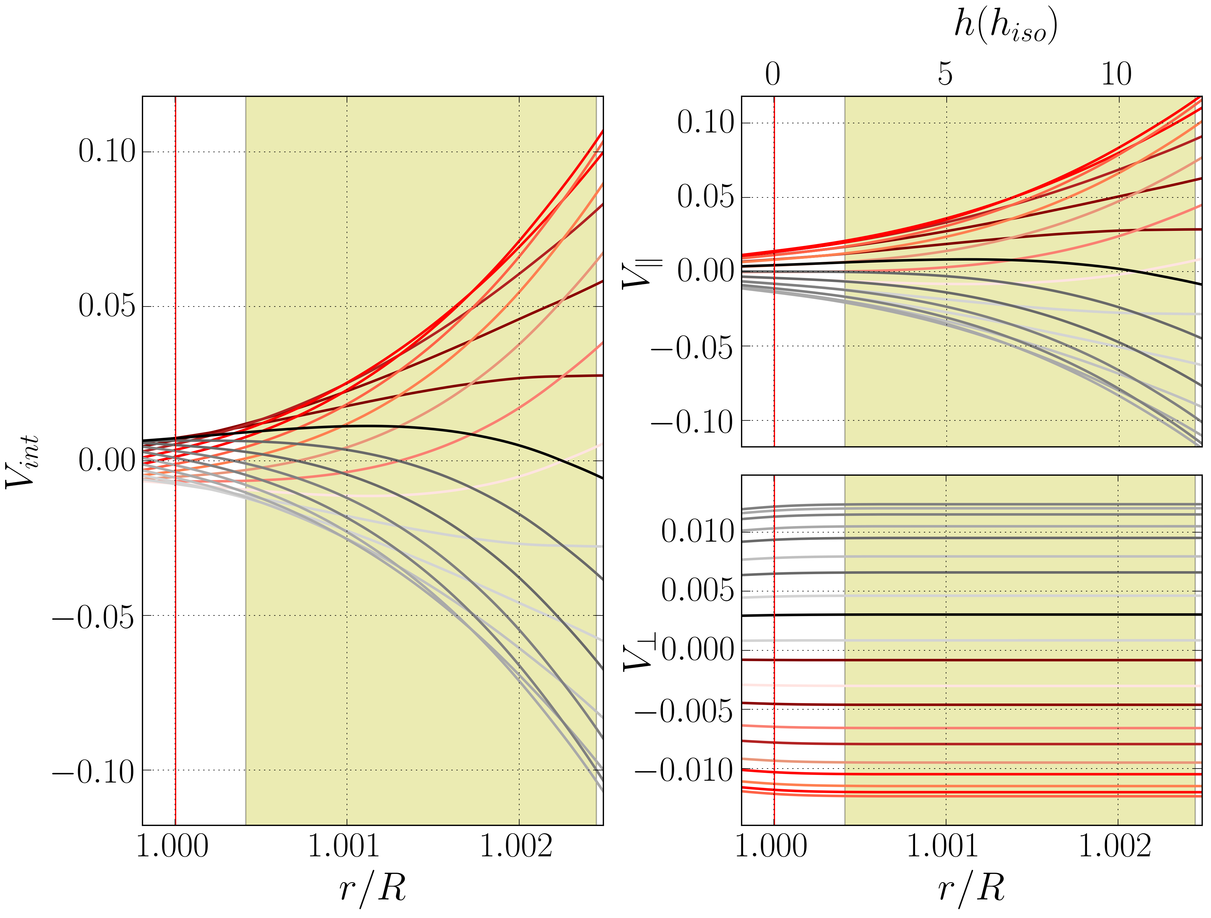
Figure 12: The same as Fig. 6 but for a mode of frequency $1.7$ mHz and degree $l=0$, a magnetic field of $2$ kG, and an observer equator-on.

Looking at Fig. 13, lower right panel, we see that similarly to case 1 the total phase (black line) follows the parallel phase (red line) in the outermost layers, and diverges from it as one approaches deeper regions of the atmosphere, due to the influence of the magnetic waves. However, contrary to case 1, the parallel phase (red line) now varies with depth, due to the contribution of the acoustic running waves that are concentrated towards the equator, where the observer is positioned. As a result, the total phase varies also in the outer atmospheric region. The phase variation can be seen also in the left panel of Fig. 13.

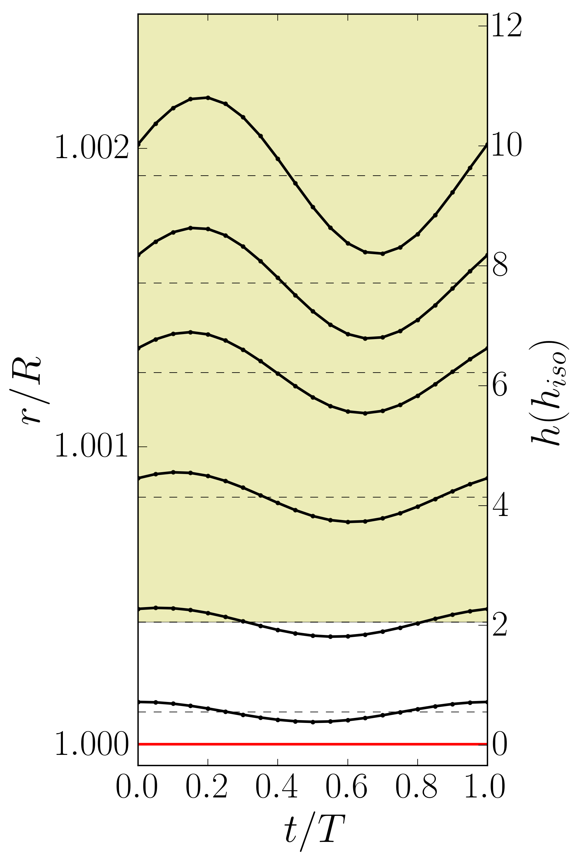
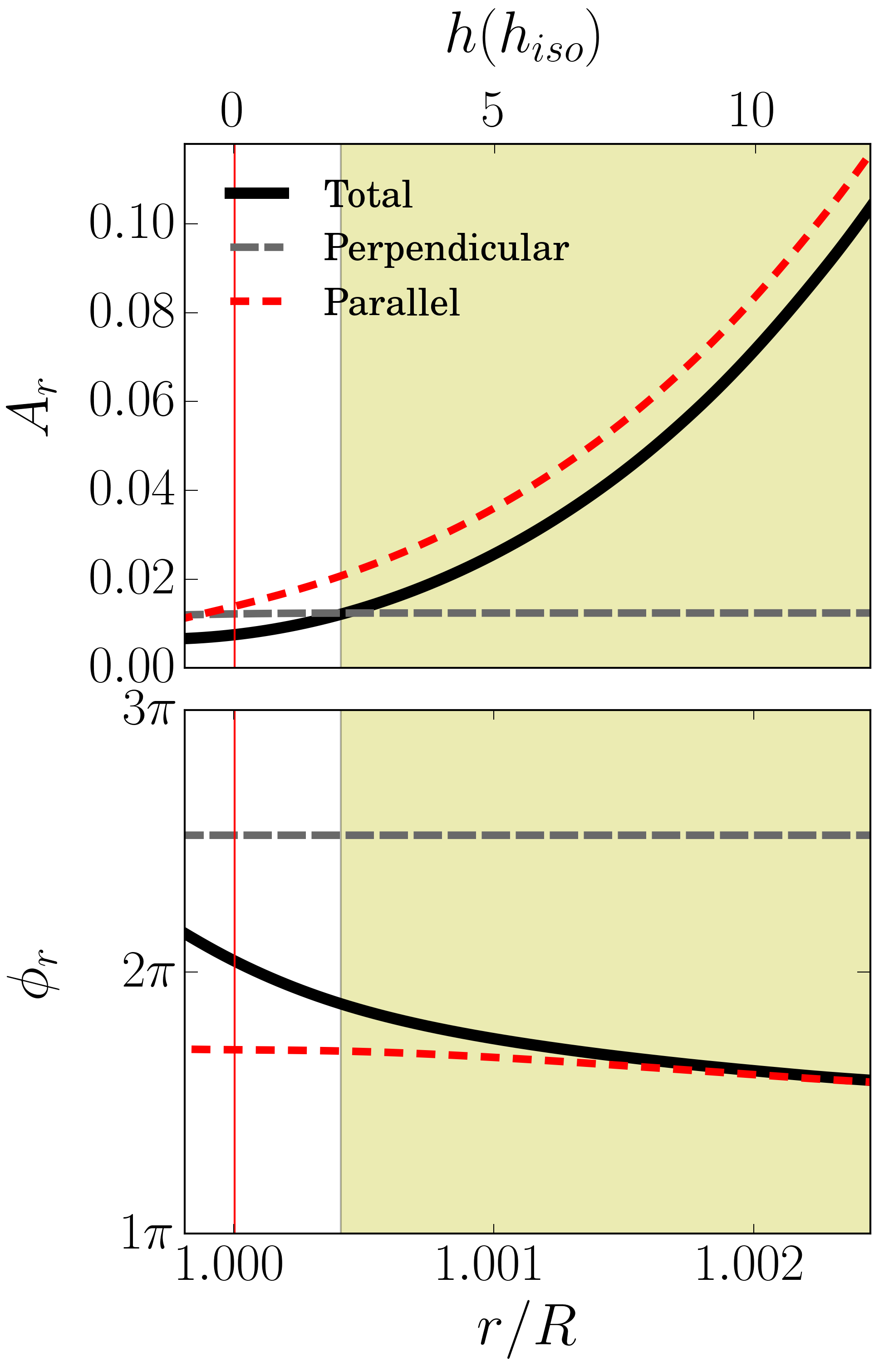
Figure 13: The same as Fig. 7 but for a mode of frequency $1.7$ mHz and degree $l=0$, a magnetic field of $2$ kG, and an observer equator-on.

3.5 Case 5

The second case with an observer equator-on is for a mode with a frequency of $2.2$ mHz and degree $l=0$ (cf. Table 2).

The radial velocity is shown in Fig. 14, left panel, and the acoustic and magnetic waves’ contributions are shown in Fig. 14, top- and bottom-right panels, respectively. In the outer atmospheric layers, the two contributions differ by 1 order of magnitude, just as in case 2, with the same frequency but a pole-on observer. Thus, the acoustic waves are dominant in those layers. While this is similar to case 2, here we can see a modulation with height of the exponential behavior in the atmosphere. This is due to the fact that in this case the observer is looking more directly at the acoustic running waves.

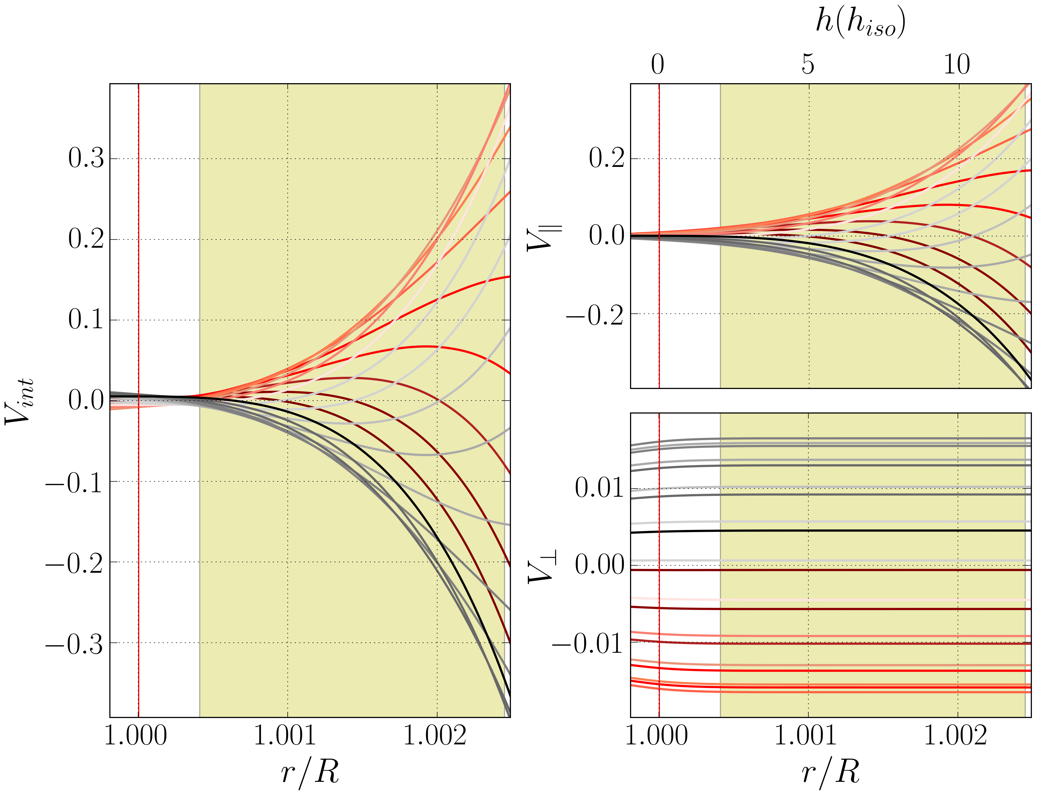
Figure 14: The same as Fig. 6 but for a mode of frequency $2.2$ mHz and degree $l=0$, a magnetic field of $2$ kG, and an observer equator-on.

The amplitude and phase variations of the radial velocity are shown in Fig. 15, right panels, where again we have the total amplitude (black line, top panel) dominated by the amplitude derived from the acoustic wave’s contribution (red line, same panel) in the high atmosphere, and a total phase (black line, bottom panel) that changes from following the phase derived from the acoustic wave’s contribution in the high atmosphere (red line, same panel) to following the phase derived from the magnetic wave’s contribution (gray line, same panel) in the inner layers of the atmosphere.

Considering Fig. 15, left panel, the change in the phase is evident and much greater than the phase variation seen in the case 2. This is again because with the pole-on view the observer is looking directly at the acoustic standing waves at the pole, but with the equator-on view the observer is looking directly at the acoustic running waves in the equator.

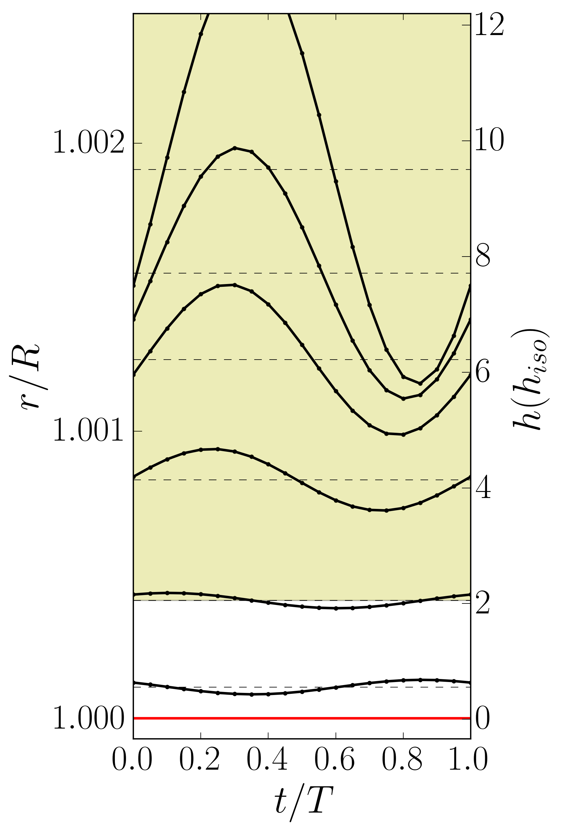
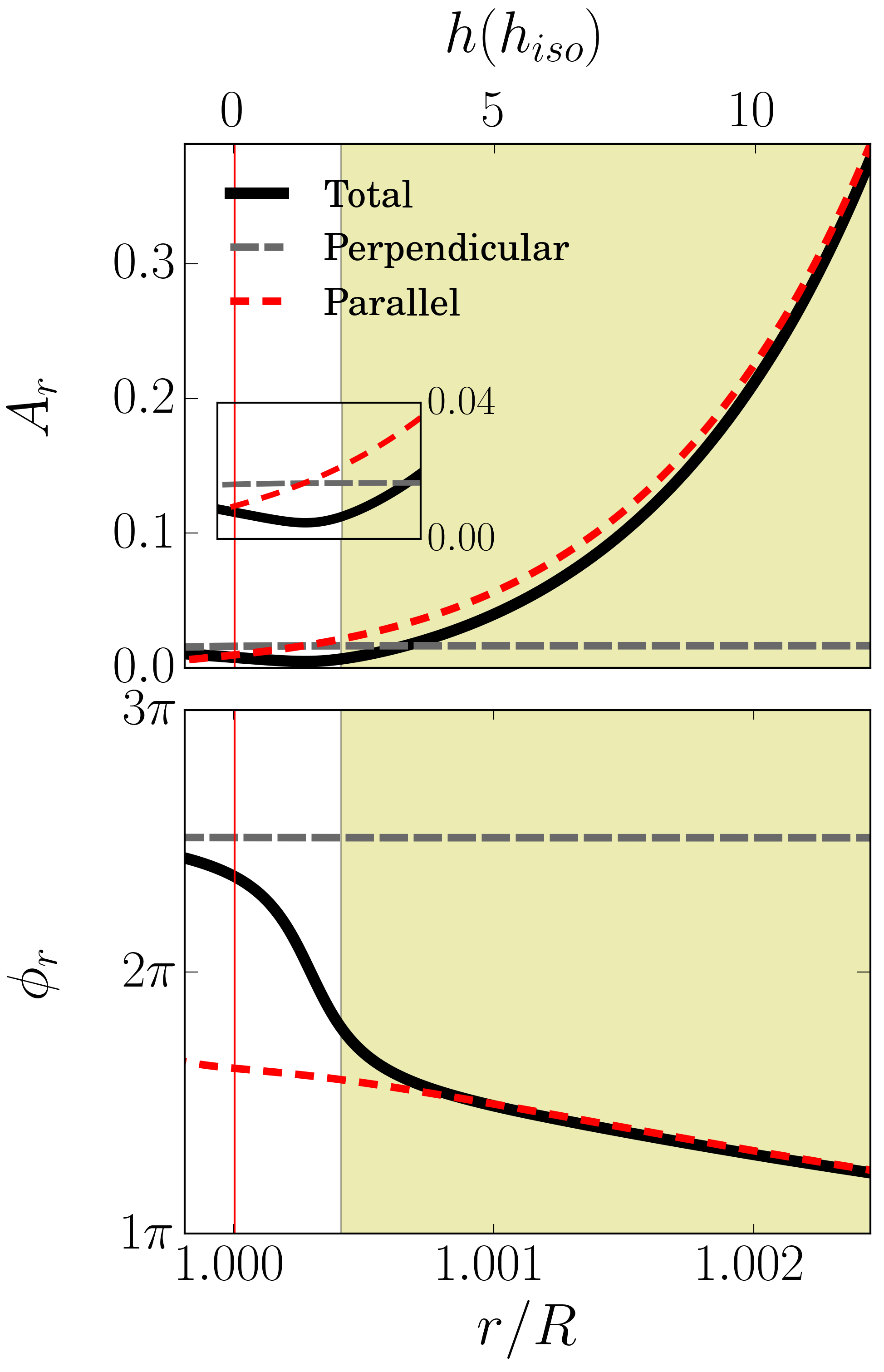
Figure 15: The same as Fig. 7 but for a mode of frequency $2.2$ mHz and degree $l=0$, a magnetic field of $2$ kG, and an observer equator-on. The close-up shows the behaviour of the amplitudes near the photosphere.

3.6 Case 6

This case is for a mode with a frequency of $2.7$ mHz, above the acoustic cut-off, and a degree $l=0$, and an equator-on observer (cf. Table 2). The radial velocity, seen in Fig. 16, left panel, shows a fast exponential growth, which is modulated with height, since the acoustic running waves are present in the full visible disk. From inspection of Fig. 16, right panels, we can see, as in the previous cases, that the contribution from the acoustic wave to the radial velocity dominates throughout most of the atmosphere, with the exception of the innermost layers.

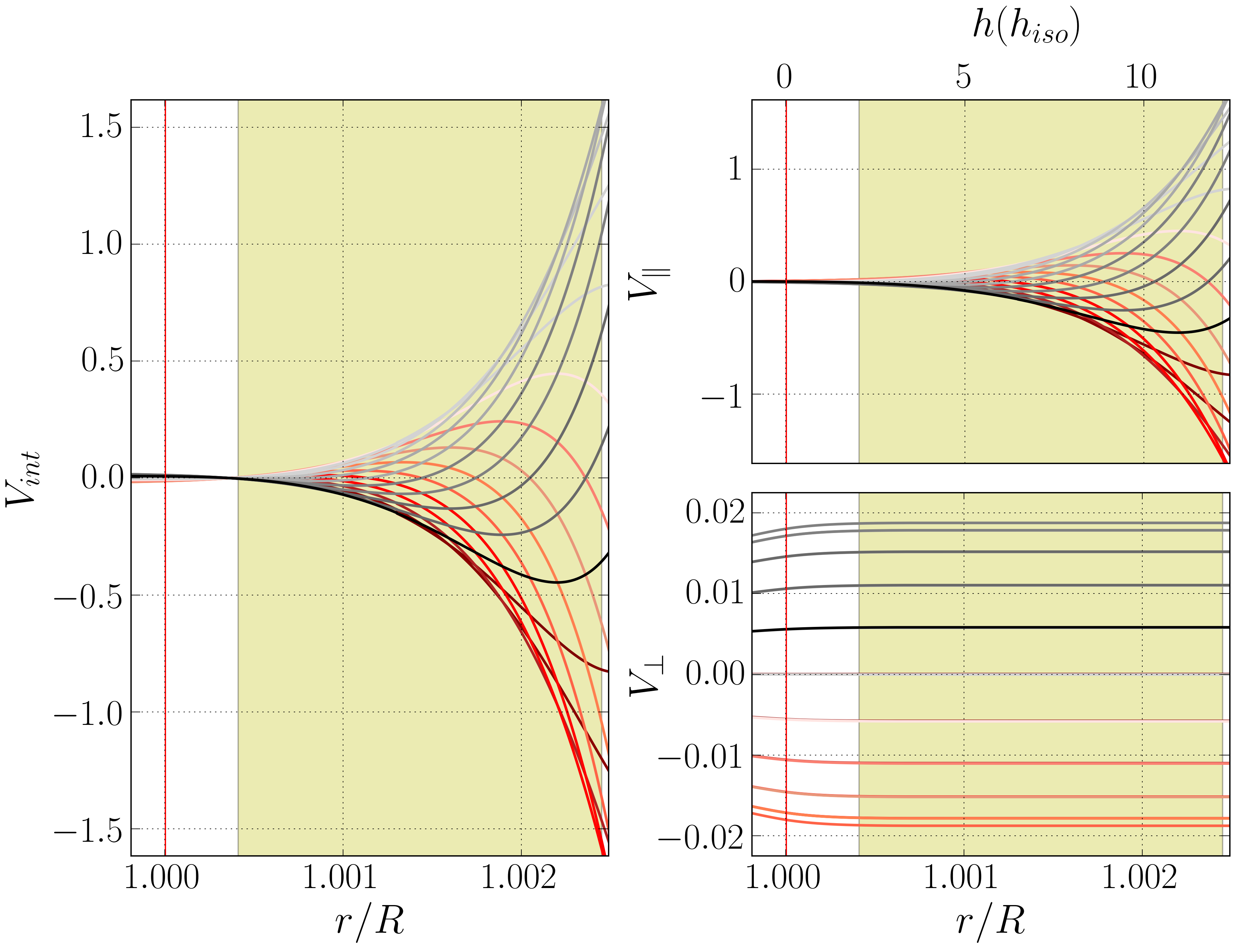
Figure 16: The same as Fig. 6 but for a mode of frequency $2.7$ mHz and degree $l=0$, a magnetic field of $2$ kG, and an observer equator-on.

Figure 17, right panels, shows the amplitude and phase variations for this case. We see a very significant phase variation (black line, bottom panel) in the isothermal atmosphere, which is mainly due to the contribution of the acoustic running waves (red line, same panel). A significant phase variation was already seen in case 3, for the same frequency, with a pole-on observer, but it is even more significant here. This is because, the acoustic running waves near the equator are propagating almost perpendicularly to the equator-on observer. Therefore, their wavenumber projection into the line-of-sight direction is very large, resulting in rapid height-variations in the center of the visible disk, which contribute significantly to the radial velocity integral. As before, in these layers the total amplitude (black line, top panel) is dominated by the acoustic wave’s contribution (red line, same panel). In the inner atmosphere we can identify a jump of $\pi$, caused by the change in the dominant contribution, from acoustic in the outer layers to magnetic in the inner layers. A phase jump had already been seen in case 3, but in this case the change is sharper. This is because here the magnetic and acoustic contributions are completely out of phase.

Although we do not illustrate it here, we have verified that this particular apparent node for a mode of this frequency and degree l=0 can be seen from any observation angle, although its exact position changes with the observer’s view.

The variation in the phase in the upper atmosphere is also very clear in Fig. 17 (left panel).

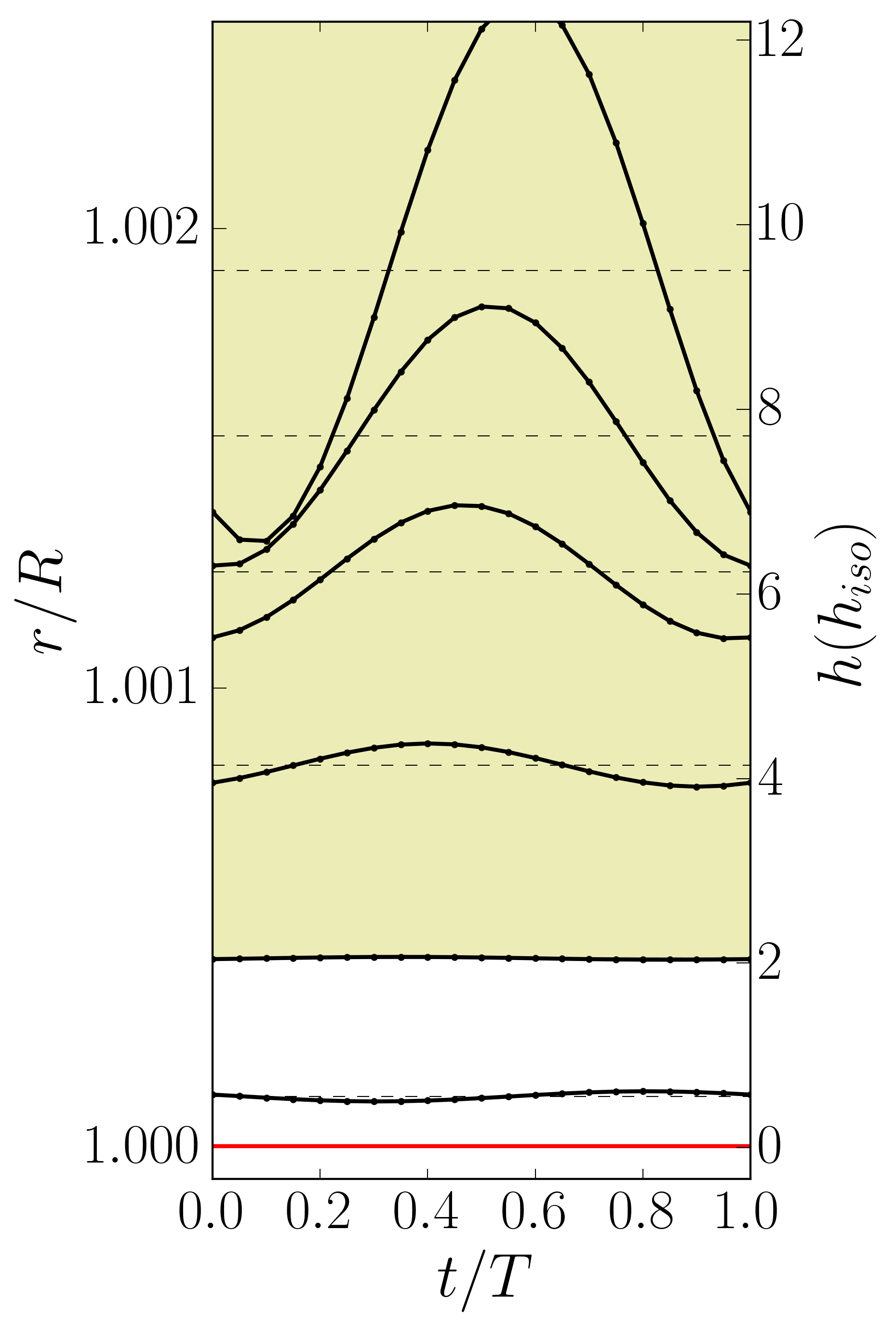
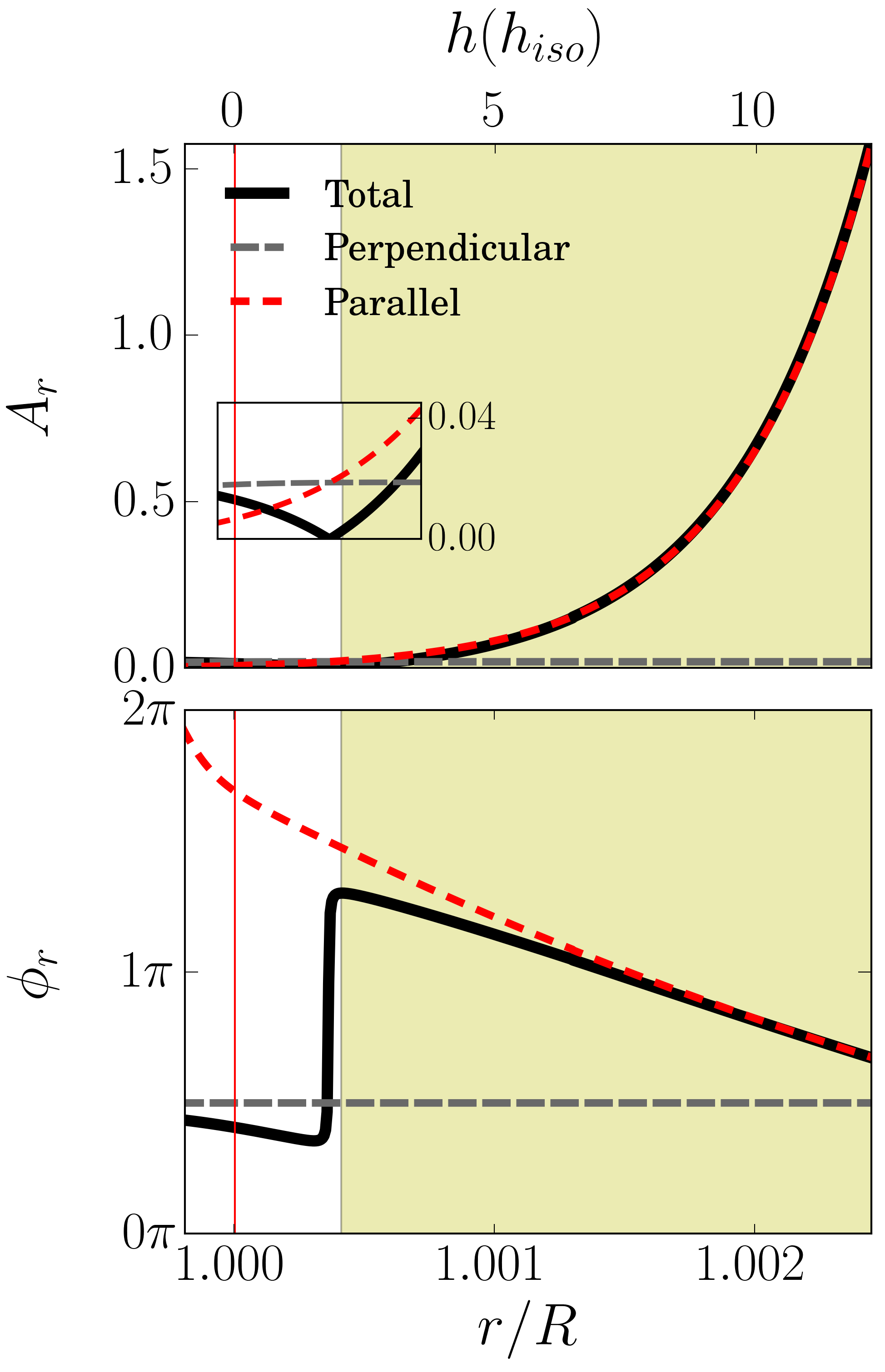
Figure 17: The same as Fig. 7 but for a mode of frequency $2.7$ mHz and degree $l=0$, a magnetic field of $2$ kG, and an observer equator-on. The close-up shows the behaviour of the amplitudes near the photosphere.

3.7 Case 7

The last case that we will consider is selected to illustrate an apparent node in the middle of the isothermal atmosphere, as first discussed by Sousa & Cunha (2011) for a toy model of a full isothermal atmosphere. This case considers a mode with a frequency of $2.7$ mHz, that is above the acoustic cut-off, and degree $l=0$, and a magnetic field of $B_{p}=2$ kG (cf. Table 2). Moreover, the observer is pole-on, and we assume the elements are concentrated around the equator, in the region defined by $53^{o}<\theta<127^{o}$, which are, thus, considered as limit angles, $\theta_{i}$ and $\theta_{f}$, for the integration in eq. (10).

The radial velocity for this case is shown in Fig. 18, left panel. In the middle of the isothermal atmosphere we can see a sudden change in the radial velocity which looks somewhat similar to what one would expect in the presence of a node.

From the inspection of the right panels of the same figure, we notice that in this case the acoustic and magnetic waves’ contributions are overall of the same order of magnitude. Thus, we can recognize in the radial velocity shown in the left panel, the exponential behavior of the acoustic waves in the upper atmosphere, but also, the constant behavior of the magnetic waves in the inner atmosphere. And like in case 6, we can see that the acoustic and magnetic waves’ contributions are out of phase, as seen by the fact that for a given time (given color line in the right panels), the acoustic (top panel) and magnetic (bottom panel) contributions have opposite sign. This leads again to a cancellation in the integral defining the radial velocity and is the cause of the apparent node.

For the stellar model used in this paper, we find this type of apparent nodes in the higher atmospheric layers when considering elements distributed around the equator. They are seen from any position, and, more commonly, for even-degree l modes.

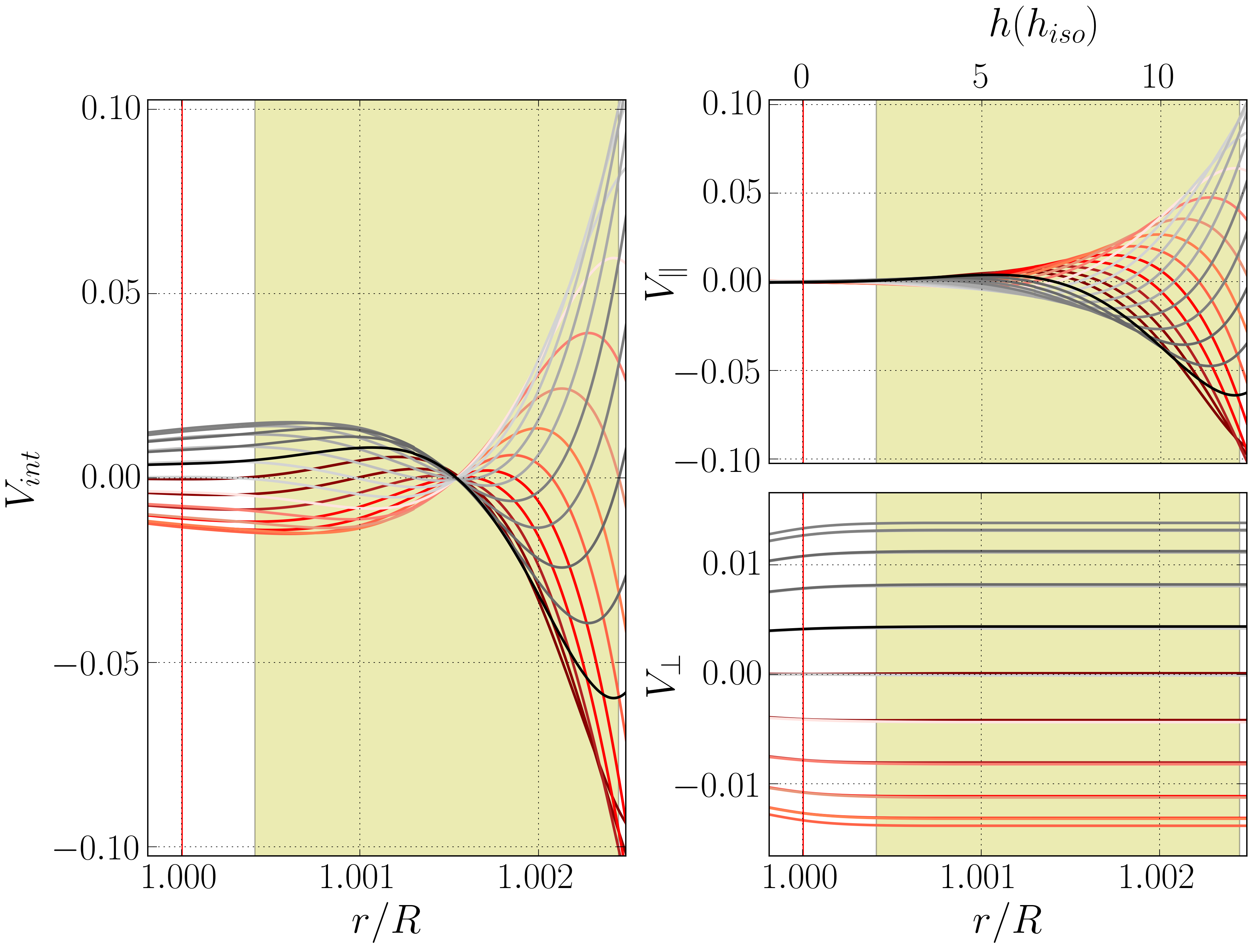
Figure 18: The same as Fig. 6 but for a mode of frequency $2.7$ mHz and degree $l=0$, a magnetic field of $2$ kG, and an observer equator-on. The integration, for this case only, is in the region defined by $53^{o}<\theta<127^{o}$.

The amplitude and phase variations are shown in Fig. 19, right panels. We see the total amplitude (black line, top panel) changing from behaving similarly to the amplitude of the acoustic wave’s contribution (red line, same panel) in the upper atmosphere to behaving like the amplitude of the magnetic wave’s contribution (gray line, same panel) in the inner atmosphere. Moreover, because the magnetic and acoustic waves’ contributions are similar in magnitude but with opposite sign, at some point in the isothermal atmosphere the total amplitude decreases, going through a local minimum. At the same location we see the total phase varying by $\pi$ (black line, bottom panel). These variations in amplitude and phase, as well as those found in cases 3 and 6 in the inner atmospheric layers, would, in an observational context, be interpreted as a presence of a node. However, this behavior is not caused by a node in a standing wave. It’s simply a visual cancellation effect between the acoustic and magnetic contributions to the radial velocity.

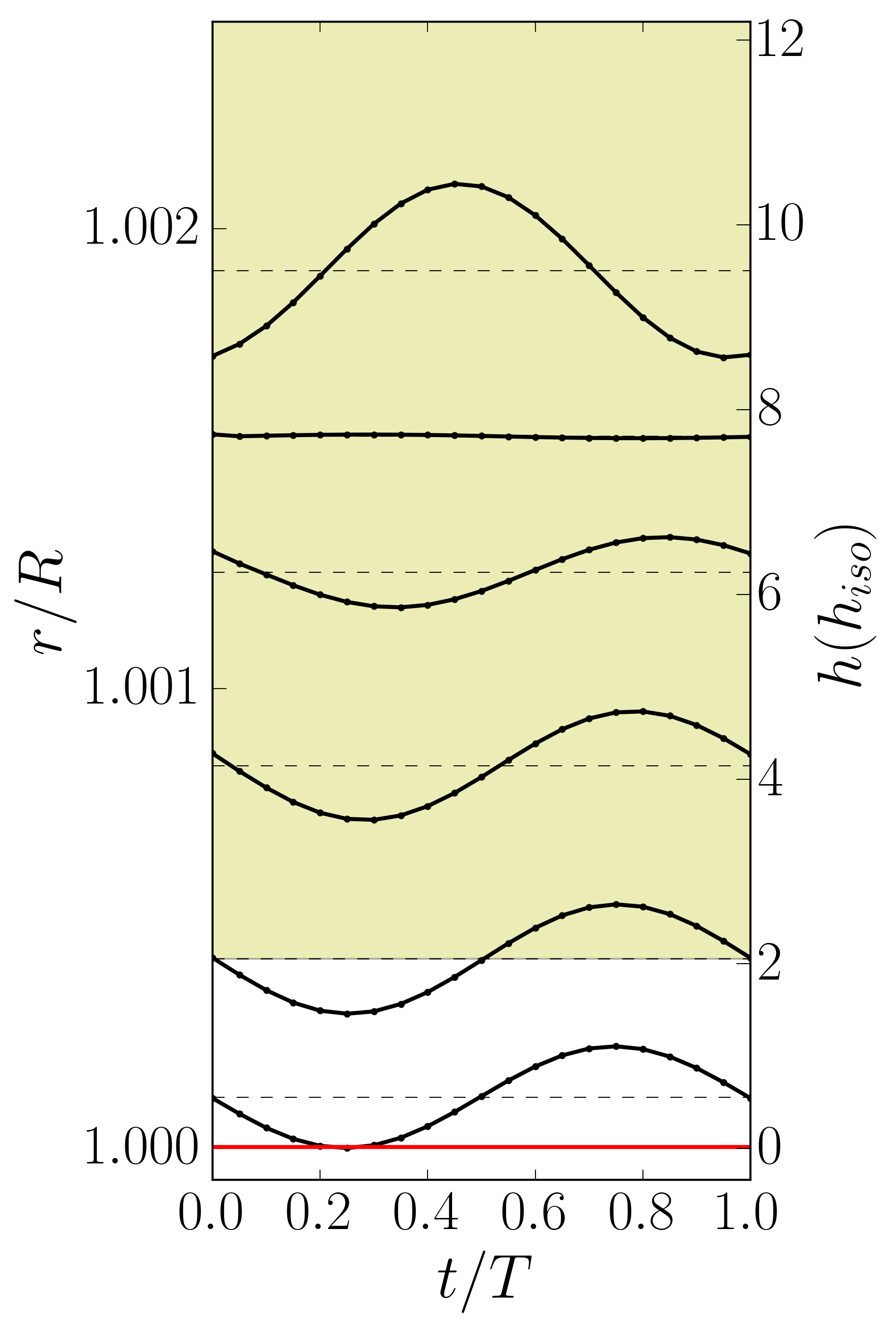
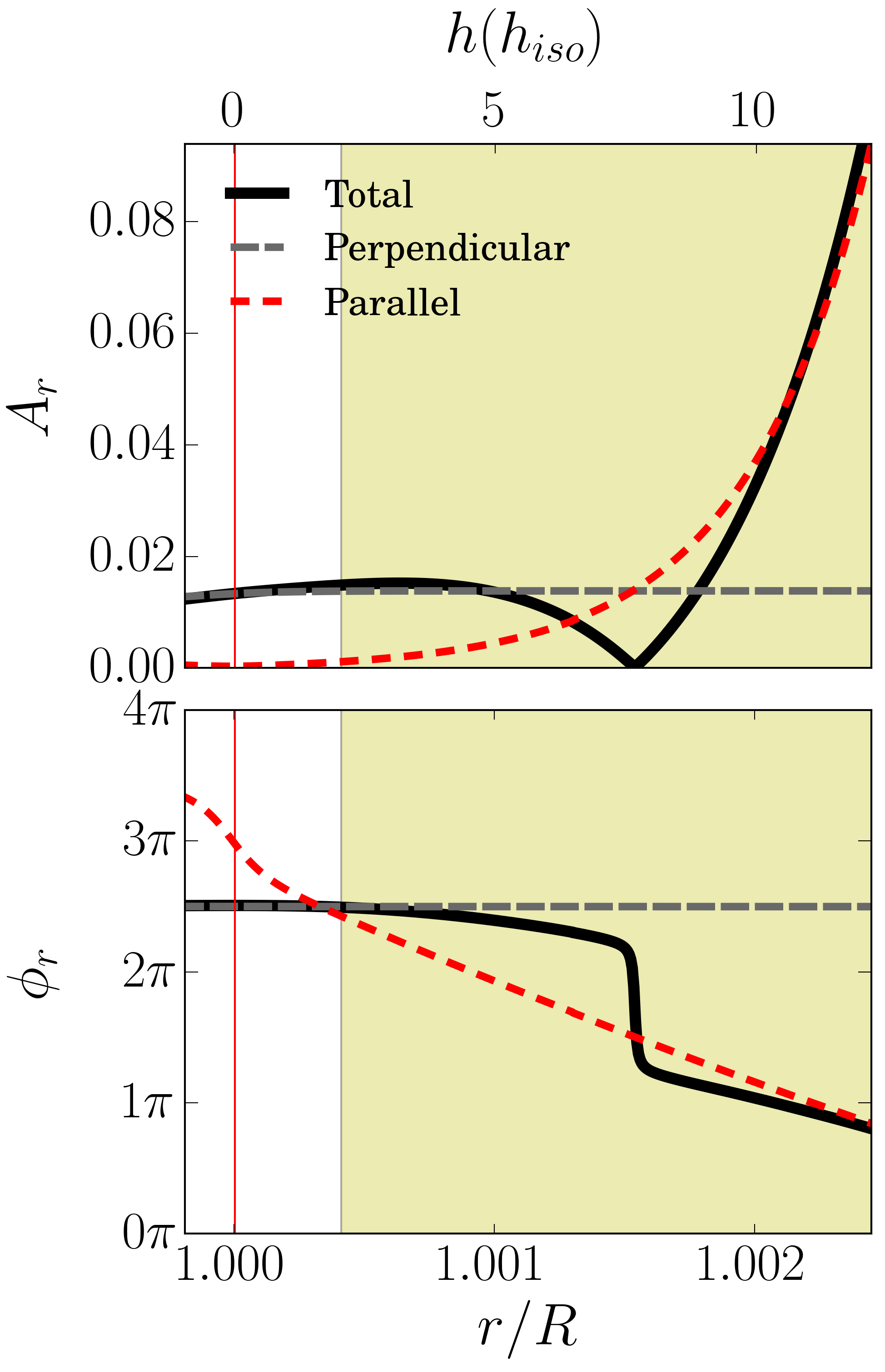
Figure 19: The same as Fig. 7 but for a mode of frequency $2.7$ mHz and degree $l=0$, a magnetic field of $2$ kG, and an observer pole-on. The integration, for this case only, is in the region defined by $53^{o}<\theta<127^{o}$.

4 Discussion and Conclusion

4.1 General behavior of the amplitude and phase

Our results show that in general the amplitude increases rapidly with height, due to the rapid increase of the amplitude of the acoustic component. How significant the increase is depends also on the frequency. As larger frequencies are considered, the radial velocity can reach greater amplitudes due to the increased presence of acoustic running waves in the atmosphere of the star. As for the phase behaviour, for frequencies below the acoustic cut-off the phase may vary due to a change in the type of waves that dominate the radial velocity integral. Moreover, depending on the position of the observer, the contribution of the acoustic waves in regions where the frequency is above the critical frequency, $\omega_{c}$, may become dominant, resulting in a change of the phase due to the running acoustic waves. When the frequency is above the acoustic cut-off, the phase is found to vary regardless of the position of the observer. Finally, we note that the position of the observer influences the phase behaviour not only because it determines the fraction of observed area where running waves are present, but also because the direction of the magnetic field around the equator makes the sound waves travel inclined to an observer that has an equator-on view, making the projection of that component of the velocity field in the direction of the observer vary on short scales.

Concerning the contributions from the acoustic and magnetic components of the wave where these are decoupled, after inspecting the six cases with integration of the entire visible disk we can note that the acoustic waves dominate the behavior of the radial velocity in the upper atmosphere for most of the cases. This is explained by the difference in the amplitude behavior of the acoustic and magnetic waves. While the first has an exponential behavior in the atmosphere, the second has a constant behavior, making the acoustic waves’ contributions dominant in the outer layers of the atmosphere.

In the inner layers of the atmosphere we see a different scenario, as the magnetic waves start to have an influence, changing the amplitude and the total phase of the radial velocity. This is the region where the change of dominance from acoustic to magnetic waves’ contribution occurs in our model, giving rise to a phase variation that in some cases may be abrupt enough to form an apparent node. The position of this node, found when integrating the whole visible disk, is expected to depend on the place where the magnetic and acoustic waves decouple (illustrated in Fig. 5 for the current model), since that decoupling determines the relative amplitude of the two components, which beyond that point have a different dependence on atmospheric height. For that reason, it is expected that the position of the node will be different for models with different global properties (e..g, different temperature).

Finally, we find that apparent nodes in the higher atmospheric layers appear often for spots or belts of elements in the equatorial area, when acoustic running waves are present. Exploring several frequencies and mode degrees we found that this phenomena can occur for any position of the observer. Also, for the node discussed in case 7 we have explored further configurations, changing the width of the belt and also the symmetry of the limits of integration, and found that the apparent node remains present, showing only slight changes either in the minimum amplitude, or in the atmospheric height position. However, it disappears when the interval over which the integration is performed is greater than $49^{o}<\theta<139^{o}$.

4.2 Comparison with the observations

Our model shows that the radial velocity amplitude increases significantly (can reach one to two orders of magnitude) throughout the atmosphere. This increase is a direct consequence of the decrease in the density, as discussed in Sousa & Cunha (2011), and it is most significant when the integral defining the radial velocity is dominated by the running acoustic waves. This is in agreement with the behaviour of the radial velocity amplitudes inferred from the observations, derived from absorption lines that are formed at different depths in the atmosphere (Ryabchikova et al., 2007a; Ryabchikova et al., 2007b; Kochukhov et al., 2008; Freyhammer et al., 2009).

In addition, our model shows that the phase variations throughout the atmosphere can take a variety of forms, that depend critically on the position of the observer and on the frequency of the modes. While in most cases the phase varies smoothly with height in the atmosphere, in some cases the variations are sharper, taking place over relatively short distances. These sharper variations can be found both in the low and high atmospheric regions, in our model, depending on the conditions. The latter case (e.g., Fig. 18 and 19, with sharp phase variations seen at densities between $\approx 10^{-9}$ and $10^{-11}$ gcm^-3), is of particular interest when comparing with the observations. Smooth, as well as sharp radial velocity phase variations are also commonly inferred from the spectroscopic time-series of roAp stars, particularly in the strongest pulsating lines that form high in the atmosphere, between optical depths of about log tau=-4 and -6 (Saio et al., 2010; Saio et al., 2012), corresponding to regions of low densities similar to that mentioned above.

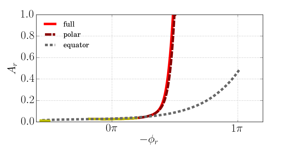
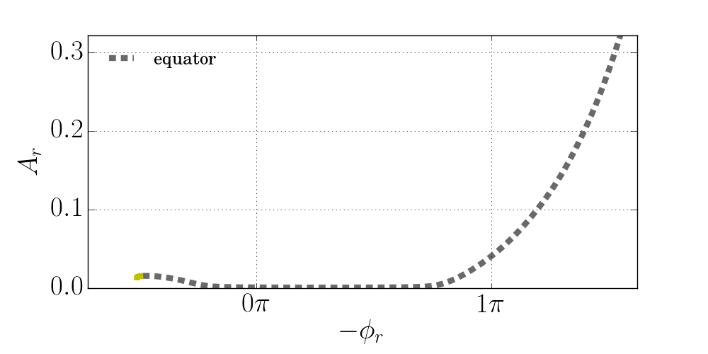
Figure 20: Amplitude versus phase variation for a magnetic field of $2$ kG. Top panel, for a mode with a frequency of $2.5$ mHz and a degree $l=0$, and an observer pole-on. Bottom panel, for a mode with a frequency of $2.7$ mHz and a degree $l=0$, and an observer pole-on. The solid red line shows the amplitude-phase variation for integration over the full visible disk, while the long dashed dark-red line shows the result for a spot around the pole and the short dashed grey line the result for an equatorial belt. The yellow part of the curves marks the region from the bottom of the photosphere to the bottom of the isothermal atmosphere. We use the negative of $\phi_{r}$ in this figure to facilitate the comparison with the observational works (e.g. Ryabchikova et al. (2007b) ), where the fit is often done to a function of the form $A_{r}\cos(\omega t-\phi_{r})$, rather than the one used in our definition (cf. eq. 12).

A common way found in the literature to analyze the observations is to combine the amplitude and phase variations in an amplitude-phase diagram. Here we perform a similar diagram based on the model results, for a chemical spot in the pole and a chemical spot in the equator. For simplicity, we shall consider that the chemical contrast is maximum, i.e., that only the regions inside the spot of a given element contribute to the radial velocity measured from that element. As we can see in Fig. 20, top panel, in the poles the variation in phase is smaller than in the equator, and also the amplitude can reach higher values. This difference between the polar spot and the equatorial spot can be seen also in the observations. As an example, in the case of the element Yttrium, Y, that is found to be more significantly shifted from the magnetic pole than, e.g., Nd and Pr (Lüftinger et al., 2010), the radial velocities are found to have a small amplitude but to show a greater variation in phase (Ryabchikova et al., 2007b), following the same behavior as the equator spot in Fig. 20. That is in contrast with the behavior found for other elements, concentrated in the polar regions, whose amplitude-phase variation behaves more like the polar spot in the same figure.

A claim found in several observational papers is that a node can sometimes be seen in the outer parts of the atmosphere of roAp stars. Based on physical grounds, in a model atmosphere like the one adopted here we do not expect a node anywhere in the outer atmosphere of the star. Even for relatively low magnetic fields, the magnetic and acoustic waves are decoupled throughout most of the atmosphere. The amplitude of the magnetic waves is constant and has a characteristic scale that is larger than the atmosphere, thus, it cannot show a node. Moreover, the amplitude of the acoustic waves, with an exponential growth, is either non-oscillatory, when the frequency is below the critical cut-off frequency $\omega_{c}$, or has an oscillatory behavior that changes with time, when the frequency is above $\omega_{c}$. Therefore, in such a model, any node detected in the outer atmosphere must be only apparent, resulting from the projection and integration of the velocity field over the visible disk or part of it. We have shown an example of how that observational illusion can occur, in the case 7. In Fig. 20, bottom panel, we can see the amplitude versus phase variation diagram for this case. The node is evident in the grey dashed line, as we can see that the amplitude first decreases, then goes through a minimum of almost a pi long over a short variation of radius, and grows back again. This kind of behavior can be seen in the amplitude versus phases diagram of 33 Lib and 10 Aql (Ryabchikova et al., 2007b; Sachkov et al., 2008).

On the other hand, true node-like features may be physically expected if sharp structural variations, capable of reflecting partially the acoustic waves, are present in the atmosphere. That kind of phenomena has been discussed in different contexts, including in the transition between the chromosphere and corona in the sun (Balmforth & Gough, 1990) and has been found in models of roAp stars presented by Saio et al. (2010); Saio et al. (2012). In the latter, the authors compare the phase and amplitude variations of models that best fit two particular roAp stars. Of particular relevance, in the first of these studies the authors discuss the impact on the phase and amplitude variations of using different atmospheric models, by comparing the results obtained with a standard Ap atmosphere, adopted from Shibahashi & Saio (1985), with those obtained with a model atmosphere that accounts for the stratification of chemical elements observed in roAp stars, adopted from Shulyak et al. (2009). The authors show that the latter model, characterized by a temperature inversion around the atmospheric layers where Nd and Pr accumulate, provides a better agreement with the observations, emphasizing the importance of using an empirical, self-consistent model atmosphere, derived specifically for the star under consideration, when attempting to perform detailed modelling of a given star. We invite the reader to have a look at the interesting discussion presented by these authors for further details.

Evidence for non-standard temperature gradients, including temperature inversions, has been found in a number of Ap stars. These abnormal temperature gradients are linked to a chemical stratification of elements, in particular a significant accumulation of REEs in the outer atmospheric layers (e.g. Shulyak et al., 2009, 2010). Moreover, possible vertical magnetic field gradients have been investigated by several studies (e.g. Nesvacil et al., 2004; Kudryavtsev & Romanyuk, 2012; Rusomarov et al., 2013; Hubrig et al., 2018). The complexity of the element distribution in the atmospheres of Ap stars and the simultaneous radial and horizontal inhomogeneities, however, render some difficulty to the interpretation of the detected magnetic field variation with height, leading, at times, to contradictory statements. For example, the presence of a radial magnetic field gradient has been corroborated by a recent study of the strongly peculiar roAp star HD 101065 (Przybylski’s star) Hubrig et al. (2018). However, no such gradient was found for another roAp star HD 24712 (Rusomarov et al., 2013). In any case, the main impact on pulsations of this complexity of the Ap stars’ atmospheric structure is expected to come from the possible sharp temperature gradients, which, as mentioned above, will induce partial reflection of the acoustic waves. In particular, that partial reflection is likely in the origin of the quasi-nodes discussed in Saio’s work.

Two stars have been argued to show a node in the atmosphere, 33 Lib and $10$ Aql (Mkrtichian et al., 2003; Elkin et al., 2008; Sachkov et al., 2008). These two stars have a main frequency above the acoustic cut-off frequency and very long rotational periods. Because of the latter the magnetic field structure and the surface distribution of elements cannot be derived making it difficult a direct comparison with our model. Nevertheless, in the light of the understanding of the problem provided by the present work we can confidently conclude that either we are in the presence of an apparent node, resulting from the cancellation effect of the acoustic and magnetic waves’ contributions to the integral, or sharp variations in the atmospheric structure of these roAp stars are capable of significantly reflecting the acoustic waves. Checking the latter possibility requires adopting a more realistic atmospheric model, which we will do in a future work.

In conclusion, we find that the behaviour of the radial velocity in our magnetic model resembles that inferred from high-resolution spectroscopic time-series of roAp stars, both in what concerns the amplitude and phase variations throughout the atmosphere. Quantitative comparisons and further test to the model shall be carried out in a follow up work directed at the modelling of particular stars, in which the atmospheric structure to adopt will be one derived from empirical self-consistent modeling of the stellar spectra.

References

- Alentiev et al. (2012) Alentiev D., Kochukhov O., Ryabchikova T., Cunha M., Tsymbal V., Weiss W., 2012, Monthly Notices of the Royal Astronomical Society: Letters, 421, L82
- Baldry et al. (1998) Baldry I., Bedding T., Viskum M., Kjeldsen H., Frandsen S., 1998, Monthly Notices of the Royal Astronomical Society, 295, 33
- Balmforth & Gough (1990) Balmforth N., Gough D., 1990, Solar Physics, 128, 161
- Balmforth et al. (2001) Balmforth N., Cunha M., Dolez N., Gough D., Vauclair S., 2001, Monthly Notices of the Royal Astronomical Society, 323, 362
- Bigot et al. (2000) Bigot L., Provost J., Berthomieu G., Dziembowski W., Goode P., 2000, Astronomy and Astrophysics, 356, 218
- Claret & Hauschildt (2003) Claret A., Hauschildt P., 2003, Astronomy & Astrophysics, 412, 241
- Cunha (2002) Cunha M. S., 2002, Monthly Notices of the Royal Astronomical Society, 333, 47
- Cunha (2006) Cunha M., 2006, Monthly Notices of the Royal Astronomical Society, 365, 153
- Cunha (2007) Cunha M., 2007, Communications in Asteroseismology, 150, 48
- Cunha & Gough (2000) Cunha M. S., Gough D., 2000, Monthly Notices of the Royal Astronomical Society, 319, 1020
- Cunha et al. (2013) Cunha M., Alentiev D., Brandão I., Perraut K., 2013, Monthly Notices of the Royal Astronomical Society, 436, 1639
- Dziembowski (1977) Dziembowski W., 1977, Acta Astronomica, 27, 203
- Dziembowski & Goode (1996) Dziembowski W., Goode P. R., 1996, The Astrophysical Journal, 458, 338
- Elkin et al. (2008) Elkin V., Kurtz D., Mathys G., 2008, Monthly Notices of the Royal Astronomical Society, 386, 481
- Freyhammer et al. (2009) Freyhammer L., Kurtz D., Elkin V., Mathys G., Savanov I., Zima W., Shibahashi H., Sekiguchi K., 2009, Monthly Notices of the Royal Astronomical Society, 396, 325
- Hubrig et al. (2018) Hubrig S., Järvinen S., Madej J., Bychkov V., Ilyin I., Schöller M., Bychkova L., 2018, Monthly Notices of the Royal Astronomical Society, 477, 3791
- Khomenko & Kochukhov (2009) Khomenko E., Kochukhov O., 2009, The Astrophysical Journal, 704, 1218
- Kochukhov (2004) Kochukhov O., 2004, The Astrophysical Journal Letters, 615, L149
- Kochukhov & Ryabchikova (2001) Kochukhov O., Ryabchikova T., 2001, Astronomy & Astrophysics, 374, 615
- Kochukhov et al. (2008) Kochukhov O., Ryabchikova T., Bagnulo S., Curto G. L., 2008, Astronomy & Astrophysics, 479, L29
- Kochukhov et al. (2009) Kochukhov O., Shulyak D., Ryabchikova T., 2009, Astronomy & Astrophysics, 499, 851
- Kudryavtsev & Romanyuk (2012) Kudryavtsev D., Romanyuk I., 2012, Astronomische Nachrichten, 333, 41
- Kurtz (1982) Kurtz D., 1982, Monthly Notices of the Royal Astronomical Society, 200, 807
- Kurtz et al. (2006) Kurtz D., Elkin V., Cunha M., Mathys G., Hubrig S., Wolff B., Savanov I., 2006, Monthly Notices of the Royal Astronomical Society, 372, 286
- Landstreet & Mathys (2000) Landstreet J., Mathys G., 2000, Astronomy and Astrophysics, 359, 213
- Lüftinger et al. (2010) Lüftinger T., Kochukhov O., Ryabchikova T., Piskunov N., Weiss W., Ilyin I., 2010, Astronomy & Astrophysics, 509, A71
- Mathys (2017) Mathys G., 2017, Astronomy & Astrophysics, 601, A14
- Matthews et al. (1988) Matthews J. M., Wehlau W. H., Walker G. A., Yang S., 1988, The Astrophysical Journal, 324, 1099
- Mkrtichian et al. (2003) Mkrtichian D. E., Hatzes A. P., Kanaan A., 2003, Monthly Notices of the Royal Astronomical Society, 345, 781
- Morel (1997) Morel P., 1997, Astronomy and Astrophysics-Supplement Series, 124, 597
- Nesvacil et al. (2004) Nesvacil N., Hubrig S., Jehin E., 2004, Astronomy & Astrophysics, 422, L51
- Nesvacil et al. (2013) Nesvacil N., Shulyak D., Ryabchikova T. A., Kochukhov O., Akberov A., Weiss W., 2013, Astronomy & Astrophysics, 552, A28
- Rusomarov et al. (2013) Rusomarov N., et al., 2013, Astronomy & Astrophysics, 558, A8
- Ryabchikova et al. (2007a) Ryabchikova T., et al., 2007a, Astronomy & Astrophysics, 462, 1103
- Ryabchikova et al. (2007b) Ryabchikova T., Sachkov M., Kochukhov O., Lyashko D., 2007b, Astronomy & Astrophysics, 473, 907
- Sachkov et al. (2008) Sachkov M., Kochukhov O., Ryabchikova T., Huber D., Leone F., Bagnulo S., Weiss W., 2008, Monthly Notices of the Royal Astronomical Society, 389, 903
- Saio (2005) Saio H., 2005, Monthly Notices of the Royal Astronomical Society, 360, 1022
- Saio & Gautschy (2004) Saio H., Gautschy A., 2004, Monthly Notices of the Royal Astronomical Society, 350, 485
- Saio et al. (2010) Saio H., Ryabchikova T., Sachkov M., 2010, Monthly Notices of the Royal Astronomical Society, 403, 1729
- Saio et al. (2012) Saio H., Gruberbauer M., Weiss W., Matthews J., Ryabchikova T., 2012, Monthly Notices of the Royal Astronomical Society, 420, 283
- Shibahashi & Saio (1985) Shibahashi H., Saio H., 1985, PASJ, 37, 245
- Shulyak et al. (2009) Shulyak D., Ryabchikova T., Mashonkina L., Kochukhov O., 2009, Astronomy & Astrophysics, 499, 879
- Shulyak et al. (2010) Shulyak D., Ryabchikova T., Kildiyarova R., Kochukhov O., 2010, Astronomy & Astrophysics, 520, A88
- Smalley et al. (2015) Smalley B., et al., 2015, Monthly Notices of the Royal Astronomical Society, 452, 3334
- Sousa & Cunha (2008a) Sousa J., Cunha M., 2008a, Contributions of the Astronomical Observatory Skalnaté Pleso, 38, 453
- Sousa & Cunha (2008b) Sousa S., Cunha M., 2008b, Monthly Notices of the Royal Astronomical Society, 386, 531
- Sousa & Cunha (2011) Sousa J., Cunha M., 2011, Monthly Notices of the Royal Astronomical Society, 414, 2576