Delay Minimization for NOMA-MEC Offloading

Abstract

This paper considers the minimization of the offloading delay for non-orthogonal multiple access assisted mobile edge computing (NOMA-MEC). By transforming the delay minimization problem into a form of fractional programming, two iterative algorithms based on Dinkelbach’s method and Newton’s method are proposed. The optimality of both methods is proved and their convergence is compared. Furthermore, criteria for choosing between three possible modes, namely orthogonal multiple access (OMA), pure NOMA, and hybrid NOMA, for MEC offloading are established.

I Introduction

The application of non-orthogonal multiple access (NOMA) to mobile edge computing (MEC) has received considerable attention recently [1, 2, 3, 4]. In particular, the superior performance of NOMA-MEC with fixed resource allocation was illustrated in [1]. In [2], a weighted sum-energy minimization problem was investigated in a multi-user NOMA-MEC system. In [3], the energy consumption of NOMA-MEC networks was minimized assuming that each user has access to multiple bandwidth resource blocks. In [4], joint power and time allocation was designed for NOMA-MEC, again with the objective to minimize the offloading energy consumption. To the best of the authors’ knowledge, the minimization of the offloading delay for NOMA-MEC has not yet been studied.

The aim of this letter is to study delay minimization for NOMA-MEC offloading. Compared to the energy minimization problems studied in [2, 3, 4], minimizing the offloading delay is more challenging, since the delay is the ratio of two rate-related functions. We first transform the formulated delay minimization problem into a form of fractional programming. However, the transformed problem is fundamentally different from the original fractional programming problem in [5]. To this end, two algorithms based on Dinkelbach’s method and Newton’s method are proposed, and their optimality is rigorously proved. While for conventional fractional programming, the two methods are equivalent, as for the problem considered in this paper, Newton’s method is proved to converge faster than Dinkelbach’s method. In addition, criteria for choosing between three possible modes, namely OMA, pure NOMA, and hybrid NOMA (H-NOMA), for MEC offloading are established. Interestingly, we find that pure NOMA can outperform H-NOMA when there is sufficient energy for MEC offloading, whereas H-NOMA always outperforms pure NOMA if the objective is to reduce the energy consumption as shown in [4].

II System Model

Consider an MEC offloading scenario, in which two users, denoted by user $m$ and user $n$, offload their computation tasks to an MEC server. Without loss of generality, assume that the two users’ tasks contain the same number of nats, denoted by $N$, and user $m$’s computation deadline, denoted by $D_{m}$ seconds, is shorter than user $n$’s, denoted by $D_{n}$ seconds, i.e., $D_{m}\leq D_{n}$.

In this work, as user $m$ has a more stringent delay requirement than user $n$, user $n$ will be served in an opportunistic manner as described in the following. In particular, user $m$’s transmit power, denoted by $P_{m}$, is set the same as in OMA, i.e., $P_{m}$ satisfies $D_{m}\ln(1+P_{m}|h_{m}|^{2})=N$, where $h_{k}$ denotes user $k$’s channel gain, $k\in\{m,n\}$. User $n$ is allowed to access the time slot of $D_{m}$ seconds allocated to user $m$, under the condition that user $m$ experiences the same rate as for OMA. As shown in [4], this can be realized if user $m$’s message is decoded after user $n$’s at the MEC server and user $n$’s data rate, denoted by $R_{n}$, during $D_{m}$ is set as follows:

$$R_{n}=\ln\left(1+\frac{P_{n,1}|h_{n}|^{2}}{P_{m}|h_{m}|^{2}+1}\right),$$ (1)

where $P_{n,1}$ denotes the power used by user $n$ during $D_{m}$. If user $n$ cannot finish its offloading within $D_{m}$, a dedicated time slot, denoted by $T_{n}$, is allocated to user $n$, and the user’s transmit power during $T_{n}$ is denoted by $P_{n,2}$. Note that the three cases with $\{P_{n,1}=0,P_{n,2}\neq 0\}$, $\{P_{n,1}\neq 0,P_{n,2}=0\}$, and $\{P_{n,1}\neq 0,P_{n,2}\neq 0\}$, correspond to OMA, pure NOMA, and H-NOMA, respectively. We note that both OMA and pure NOMA can be viewed as special cases of H-NOMA. However, in this paper, the three modes are considered separately and H-NOMA is restricted to the case with $\{P_{n,1}\neq 0,P_{n,2}\neq 0\}$. Similar to [2, 3, 4], the time and energy costs for the users to download the computation outcomes from the MEC server are omitted, as they are negligibly small compared to the considered uploading costs.

III NOMA-Assisted MEC Offloading

The considered opportunistic strategy can guarantee that user $m$’s delay performance in NOMA is the same as that in OMA, and the problem for minimizing user $n$’ delay can be formulated as follows:

$$\underset{P_{n,1},P_{n,2}}{\text{ minimize}}\quad D_{m}+T_{n}$$ (2a)

s.t. $$\left\{P_{n,1}P_{n,2}\right\}\in\mathcal{S},$$ (2b)

where $T_{n}=\frac{N-D_{m}\ln\left(1+\frac{P_{n,1}|h_{n}|^{2}}{P_{m}|h_{m}|^{2}+1}\right)}{\ln\left(1+|h_{n}|^{2}P_{n,2}\right)}$,

$$\mathcal{S}=\{D_{m}P_{n,1}+T_{n}P_{n,2}\leq E,P_{n,1}\geq 0,P_{n,2}\geq 0,T_{n}\geq 0\},$$ (3)

and $E$ is user $n$’s energy constraint. We note that $T_{n}$ is zero if pure NOMA is used, and the constraint in Eq. (2b) implies that user $n$’s power during $D_{m}$ needs to ensure that user $m$ experiences the same rate as in OMA. Define $E_{1}=D_{m}\left(e^{\frac{N}{D_{m}}}-1\right)|h_{n}|^{-2}$ and $E_{2}=D_{m}\left(e^{\frac{N}{D_{m}}}-1\right)e^{\frac{N}{D_{m}}}|h_{n}|^{-2}$. The optimal power allocation policy depends on how much energy is available as shown in the following subsections.

III-A Case $E\geq E_{2}$

This corresponds to the case with sufficient energy at user $n$ for MEC offloading, and the minimal $D_{m}$ can be achieved by using pure NOMA, i.e., $P_{n,2}=0$. The condition for adopting pure NOMA is shown in the following. Since $P_{n,2}=0$, all the energy is consumed during the NOMA phase to minimize the delay, which means $P_{n,1}=\frac{E}{D_{m}}$. Hence, user $n$ is able to offload its task within $D_{m}$ if

$$N\leq D_{m}\ln\left(1+\frac{P_{n,1}|h_{n}|^{2}}{P_{m}|h_{m}|^{2}+1}\right)$$

$$\overset{(a)}{=} D_{m}\ln\left(1+e^{-\frac{N}{D_{m}}}\frac{E}{D_{m}}|h_{n}|^{2}\right),$$ (4)

where step (a) is obtained by assuming that user $m$’s power, $P_{m}$, satisfies the constraint $D_{m}\ln\left(P_{m}|h_{m}|^{2}+1\right)=N$. By solving the inequality in (4), the condition $E\geq E_{2}$ can be obtained.

The performance gain of NOMA-MEC over OMA-MEC is obvious in this case since user $n$’s delay in OMA is $D_{m}+\frac{N}{\ln\left(1+|h_{n}|^{2}P_{n,2}\right)}$ which is strictly larger than $D_{m}$. However, the comparison between OMA and NOMA becomes more complicated for the energy-constrained cases.

III-B Case $E_{1}<E<E_{2}$

This corresponds to the case, where there is not sufficient energy at user $n$ to support pure NOMA. Note that both H-NOMA and OMA are still applicable. Due to the space limit, we focus on H-NOMA ($P_{n,i}\neq 0$, $i\in\{1,2\}$), as the OMA solution can be obtained in a straightforward manner.

Note that $T_{n}$ is the ratio of two functions of $P_{n,1}$ and $P_{n,2}$, respectively, which motivates the use of fractional programming. However, compared to conventional fractional programming in [5], the problem in (2) is more challenging since the fractional function $T_{n}$ does not only appear in the objective function but also in the constraint. Two iterative algorithms will be developed based on the following Dinkelbach’s auxiliary function parameterized by $\mu$:

$$F(\mu)= \underset{P_{n,1},P_{n,2}}{\text{maxmize}}\quad\ln\left(1+|h_{n}|^{2}P_{n,2}\right)$$ (5)

$$-\mu\left(N-D_{m}\ln\left(1+e^{-\frac{N}{D_{m}}}P_{n,1}|h_{n}|^{2}\right)\right),$$

where $\left\{P_{n,1},P_{n,2}\right\}\in\tilde{\mathcal{S}}(\mu)$ and

$$\tilde{\mathcal{S}}(\mu)=\left\{D_{m}P_{n,1}+\mu^{-1}P_{n,2}\leq E,P_{n,1}\geq 0,P_{n,2}\geq 0\right\}.$$ (6)

Different from the original form in [5], the constraint set $\tilde{\mathcal{S}}(\mu)$ for the auxiliary function is also a function of $\mu$ and $F(\mu)$ might have more than one root.

For a fixed $\mu$, the following lemma provides the optimal H-NOMA solution for problem (5).

$\mathbf{Lemma}$ 1.

For a fixed $\mu$, the optimal H-NOMA power allocation policy for problem (5) is given by

$$\left\{\begin{array}[]{rl}P_{n,1}^{*}(\mu)&=\frac{E-\mu^{-1}\left(e^{\frac{N}{D_{m}}}-1\right)|h_{n}|^{-2}}{D_{m}+\mu^{-1}}\\ P_{n,2}^{*}(\mu)&=\frac{E+D_{m}\left(e^{\frac{N}{D_{m}}}-1\right)|h_{n}|^{-2}}{D_{m}+\mu^{-1}}\end{array}\right..$$ (9)

Proof.

Due to the space limit, only a sketch of the proof is provided. It is straightforward to show that problem (5) is convex for a fixed $\mu$. Hence the Karush-Kuhn-Tucker (KKT) can be applied to find the optimal solution as follows: [6]

$$\left\{\begin{array}[]{rl}-\frac{\mu D_{m}e^{-\frac{N}{D_{m}}}|h_{n}|^{2}}{1+e^{-\frac{N}{D_{m}}}P_{n,1}|h_{n}|^{2}}+\lambda_{1}D_{m}-\lambda_{2}-\lambda_{3}&=0\\ -\frac{|h_{n}|^{2}}{1+|h_{n}|^{2}P_{n,2}}+\lambda_{1}\mu^{-1}-\lambda_{2}-\lambda_{3}&=0\\ D_{m}P_{n,1}+\mu^{-1}P_{n,2}&\leq E\\ \lambda_{1}\left(D_{m}P_{n,1}+\mu^{-1}P_{n,2}-E\right)&=0\\ P_{n,i}&\geq 0,\forall i\in\{1,2\}\\ \lambda_{i}P_{n,i}&=0,\forall i\in\{2,3\}\\ \lambda_{i}&\geq 0,\forall i\in\{1,2,3\}\end{array}\right.,$$ (17)

where $\lambda_{i}$ are Lagrange multipliers. For the H-NOMA case, $P_{n,1}>0$ and $P_{n,2}>0$, and hence $\lambda_{2}=0$ and $\lambda_{3}=0$ due to constraints $\lambda_{i}P_{n,i}=0,\forall i\in\{2,3\}$. Therefore, the KKT conditions can be simplified as follows:

$$\left\{\begin{array}[]{rl}-\frac{\mu D_{m}e^{-\frac{N}{D_{m}}}|h_{n}|^{2}}{1+e^{-\frac{N}{D_{m}}}P_{n,1}|h_{n}|^{2}}+\lambda_{1}D_{m}&=0\\ -\frac{|h_{n}|^{2}}{1+|h_{n}|^{2}P_{n,2}}+\lambda_{1}\mu^{-1}&=0\\ D_{m}P_{n,1}+\mu^{-1}P_{n,2}&\leq E\\ \lambda_{1}\left(D_{m}P_{n,1}+\mu^{-1}P_{n,2}-E\right)&=0\\ P_{n,i}&\geq 0,\forall i\in\{1,2\}\\ \lambda_{1}&\geq 0\end{array}\right..$$ (24)

Due to constraint $-\frac{|h_{n}|^{2}}{1+|h_{n}|^{2}P_{n,2}}+\lambda_{1}\mu^{-1}=0$, we have $\lambda_{1}\neq 0$ for the optimal solution, otherwise $\frac{|h_{n}|^{2}}{1+|h_{n}|^{2}P_{n,2}}=0$ which cannot be true. Since $\lambda_{1}\neq 0$ and $\lambda_{1}\left(D_{m}P_{n,1}+\mu^{-1}P_{n,2}-E\right)=0$, we have $D_{m}P_{n,1}+\mu^{-1}P_{n,2}-E=0$. With some algebraic manipulations, the lemma can be proved. ∎

Remark 1: By substituting $P_{n,1}^{*}(\mu)$ and $P_{n,2}^{*}(\mu)$ into (5), $F(\mu)$ can be expressed as an explicit function of $\mu$. Unlike [5], $F(\mu)$ is not convex and may have multiple roots, which result in fundamental changes to the proof of convergence of Dinkelbach’s method.

Although $F(\mu)$ is different from the form in [5], a modified Dinkelbach’s method can still be developed as shown in Algorithm 1. In Algorithm 1, $\delta$ denotes a small positive threshold. In addition, a Newton’s method-based iterative algorithm can also be developed as in Algorithm 2, where $F^{\prime}(\mu)$ denotes the first order derivative of $F(\mu)$.

Algorithm 1 Dinkelbach’s Method Based Algorithm

1:Set $t=0$, $\mu_{0}=+\infty$ , $\delta\rightarrow 0$.

2:while  $F(\mu_{t})<-\delta$  do

3:     $t=t+1$.

4:     Update $P_{n,1}^{t}$ and $P_{n,2}^{t}$ by using $\mu_{t-1}$ and (9).

5:     Update $F(\mu_{t})$ by using $P_{n,1}^{t}$ and $P_{n,2}^{t}$.

6:     Update $\mu_{t}$ as $\mu_{t}=\frac{\ln\left(1+|h_{n}|^{2}P^{t}_{n,2}\right)}{N-D_{m}\ln\left(1+e^{-\frac{N}{D_{m}}}P_{n,1}^{t}|h_{n}|^{2}\right)}$

7:end

8:$P_{n,1}^{*}=P_{n,1}^{t}$ and $P_{n,2}^{*}=P_{n,2}^{t}$.

Algorithm 2 Newton’s Method Based Algorithm

1:Set $t=0$, $\mu_{0}=+\infty$, $\delta\rightarrow 0$.

2:while  $F(\mu_{t})<-\delta$  do

3:     $t=t+1$.

4:     Update $\mu_{t+1}=\mu_{t}-\frac{F(\mu_{t})}{F^{\prime}(\mu_{t})}$.

5:end

6:$P_{n,1}^{*,N}$ and $P_{n,2}^{*,N}$ are obtained by using $\mu_{t}$ and (9).

The following theorem confirms the optimality of the two developed algorithms.

Theorem 1.

The two iterative algorithms shown in Algorithms 1 and 2 converge to the same optimal solution of problem (2).

Proof.

We start the proof by first studying the roots of the function in (5) which can potentially be the optimal solution. We note that the steps provided in [5] cannot be straightforwardly applied to prove the optimality of the modified Dinkelbach’s method since $F(\mu)$ may have multiple roots.

Step 1 of the proof is to show the existence and uniqueness of the root of $F(\mu)$, for $\left(e^{\frac{N}{D_{m}}}-1\right)|h_{n}|^{-2}E^{-1}<\mu<\infty$. To prove this, it is sufficient to show that 1): $F(\mu)$ is strictly concave, 2): $F(\mu)=-\infty$ for $\mu\rightarrow+\infty$ and 3): $F(\mu)>0$ for $\mu\rightarrow\left(e^{\frac{N}{D_{m}}}-1\right)|h_{n}|^{-2}E^{-1}$.

The first order derivative of $F(\mu)$ is given by

$$F^{\prime}(\mu)= \left.\frac{|h_{n}|^{2}E+D_{m}\left(e^{\frac{N}{D_{m}}}-1\right)}{e^{\frac{N}{D_{m}}}D_{m}\mu+|h_{n}|^{2}E\mu+1}-\right[N-D_{m}$$ (25)

$$\left.\times\ln\left(1+e^{-\frac{N}{D_{m}}}|h_{n}|^{2}\frac{E-\frac{\left(e^{\frac{N}{D_{m}}}-1\right)|h_{n}|^{-2}}{\mu}}{D_{m}+\frac{1}{\mu}}\right)\right].$$

Unlike [5], $F^{\prime}(\mu)$ is neither strictly negative nor positive. The second order derivative of $F(\mu)$ is given by

$$F^{\prime\prime}(\mu)= \frac{\left(D_{m}^{2}-\left(e^{\frac{N}{D_{m}}}D_{m}+|h_{n}|^{2}E\right)^{2}\right)}{\left(e^{\frac{N}{D_{m}}}D_{m}\mu+|h_{n}|^{2}E\mu+1\right)^{2}(\mu D_{m}+1)}.$$ (26)

Since $e^{\frac{N}{D_{m}}}>1$ and $|h_{n}|^{2}E>0$, we have

$$F^{\prime\prime}(\mu)<0,$$ (27)

which means that $F(\mu)$ is a strictly concave function of $\mu$.

When $\mu\rightarrow\left(e^{\frac{N}{D_{m}}}-1\right)|h_{n}|^{-2}E^{-1}$, the H-NOMA solution approaches $P_{n,1}^{*}(\mu)\rightarrow 0$ and $P_{n,2}^{*}(\mu)\rightarrow\left(e^{\frac{N}{D_{m}}}-1\right)|h_{n}|^{-2}$. Consequently, $F(\mu)$ can be approximated as follows:

$$F(\mu)\rightarrow \ln\left(1+|h_{n}|^{2}\frac{E\mu+\mu D_{m}\left(e^{\frac{N}{D_{m}}}-1\right)|h_{n}|^{-2}}{D_{m}\mu+1}\right)$$

$$-\mu N$$

$$\rightarrow \frac{N}{D_{m}}-\frac{N\left(e^{\frac{N}{D_{m}}}-1\right)|h_{n}|^{-2}}{E}.$$ (28)

As suggested by the title of Section III-B, it is assumed that $E>E_{1}$, which means

$$F(\mu)>0,$$ (29)

for $\mu\rightarrow\left(e^{\frac{N}{D_{m}}}-1\right)|h_{n}|^{-2}E^{-1}$.

When $\mu\rightarrow\infty$, $F(\mu)$ can be approximated as follows:

$$F(\mu)\rightarrow \ln\left(1+|h_{n}|^{2}\frac{E+D_{m}\left(e^{\frac{N}{D_{m}}}-1\right)|h_{n}|^{-2}}{D_{m}}\right)$$ (30)

$$- \mu\left(N-D_{m}\ln\left(1+e^{-\frac{N}{D_{m}}}|h_{n}|^{2}\frac{E}{D_{m}}\right)\right)\rightarrow-\infty,$$

where the last step is obtained since for H-NOMA $\left(N-D_{m}\ln\left(1+e^{-\frac{N}{D_{m}}}|h_{n}|^{2}\frac{E}{D_{m}}\right)\right)>0$. Combining (27), (29), and (30), the proof for the first step is complete. The unique root of $F(\mu)$ for $\mu>\left(e^{\frac{N}{D_{m}}}-1\right)|h_{n}|^{-2}E^{-1}$ is denoted by $\mu^{*}$, where $\mu^{*}>\left(e^{\frac{N}{D_{m}}}-1\right)|h_{n}|^{-2}E^{-1}$.

Step 2 is to show that $T_{n}^{*}\triangleq\frac{1}{\mu^{*}}$ is the optimal solution of problem (2). This step can be proved by using contradiction. Assume that the optimal solution of problem (2) is smaller than $T_{n}^{*}$, denoted by $\bar{T}_{n}^{*}$. Denote $\bar{\mu}^{*}=\frac{1}{\bar{T}_{n}^{*}}$ and hence $\bar{\mu}^{*}>\mu^{*}$. Following steps similar to those in [5], we have $F(\bar{\mu}^{*})=0$, i.e., $\bar{\mu}^{*}$ is also a root of $F(\mu)$ and $\bar{\mu}^{*}>\mu^{*}>\left(e^{\frac{N}{D_{m}}}-1\right)|h_{n}|^{-2}E^{-1}$, which contradicts the uniqueness of the root of $F(\mu)$. Step 2 means that finding the optimal solution of problem (2) is equivalent to finding the largest root of $F(\mu)$. Therefore, the optimality of Newton’s method can be straightforwardly shown, and in the following, we only focus on the modified Dinkelbach’s method.

Step 3 is to show $F(\mu)$ is a strictly decreasing function of $\mu$, for $\mu^{*}\leq\mu\leq\infty$, which can be proved by using the facts that $\mu^{*}$ is the unique root of $F(\mu)$ for $\mu>\left(e^{\frac{N}{D_{m}}}-1\right)|h_{n}|^{-2}E^{-1}$, and $F(\mu)$ is concave.

Step 4 is to show $F(\mu_{t+1})<0$ if $F(\mu_{t})<0$ for the modified Dinkelbach’s method. Since $F(\mu_{t})<0$ and $F(\mu)$ is a strictly decreasing function for $\mu\geq\mu^{*}$, we have $\mu_{t}>\mu^{*}$. The convergence analysis for Newton’s method is provided first to facilitate that of Dinkelbach’s method. The quadratic convergence analysis for Newton’s method yields the following [7]

$$\mu^{*}-\mu_{t+1}=-\frac{F^{\prime\prime}(\mu_{\xi})}{2F^{\prime}(\mu_{t})}(\mu^{*}-\mu_{t})^{2},$$ (31)

where $\mu^{*}\leq\mu_{\xi}\leq\mu_{t}$. Note that $F^{\prime}(\mu_{t})<0$ and $F^{\prime\prime}(\mu_{\xi})<0$. Therefore, we have

$$\mu^{*}-\mu_{t+1}<0,$$ (32)

which means $F(\mu_{t+1})<0$ for Newton’s method.

For Dinkelbach’s method, $F(\mu)$ is first expressed as $F(\mu)=A(\mu)-\mu B(\mu)$, which means that $\mu$ is updated as follows:

$$\mu_{t+1}=\frac{A(\mu_{t})}{B(\mu_{t})}=\mu_{t}+\frac{F(\mu_{t})}{B(\mu_{t})}.$$ (33)

Recall that Newton’s method updates $\mu$ as follows:

$$\mu_{t+1}=\mu_{t}-\frac{F(\mu_{t})}{F^{\prime}(\mu_{t})}=\mu_{t}+\frac{F(\mu_{t})}{B(\mu_{t})-(A^{\prime}(\mu_{t})-\mu_{t}B^{\prime}(\mu_{t}))}.$$ (34)

From (25), $A^{\prime}(\mu_{t})-\mu_{t}B^{\prime}(\mu_{t})$ can be expressed as follows:

$$A^{\prime}(\mu_{t})-\mu_{t}B^{\prime}(\mu_{t})=\frac{|h_{n}|^{2}E+D_{m}\left(e^{\frac{N}{D_{m}}}-1\right)}{e^{\frac{N}{D_{m}}}D_{m}\mu+|h_{n}|^{2}E\mu+1}>0.$$ (35)

Note that $B(\mu)>(A^{\prime}(\mu_{t})-\mu_{t}B^{\prime}(\mu_{t}))>0$ since $F^{\prime}(\mu_{t})<0$. Therefore, the step size of Newton’s method is larger than that of Dinkelbach’s method. In other words, starting with the same $\mu_{t}$, $\mu_{t+1}$ obtained from Newton’s method is smaller than that of Dinkelbach’s method, which means $F(\mu_{t+1})<0$ also holds for Dinkelbach’s method.

Step 5 is to show $\mu_{t+1}<\mu_{t}$, which can be proved by using (33) and (34). An interesting property by Steps 4 and 5 is that if the initial value of $\mu$ is set as $\infty$, $\mu_{t}$ is decreasing and approaches $\mu^{*}$ as the number of iterations increases, but will never pass $\mu^{*}$, as $F(\mu_{t})$ is always negative.

Step 6 is to show that Dinkelbach’s method converges to $\mu^{*}$. This can be proved by contradiction. Assume that the iterative algorithm converges to $\breve{\mu}$, i.e., $\underset{t\rightarrow\infty}{\lim}\mu_{t}=\breve{\mu}$ and $\breve{\mu}\neq\mu^{*}$. Although $F(\mu)$ might have more than one root, $F(\mu_{t})$ is always negative if $\mu_{0}=\infty$, as illustrated by Step 4. Therefore, $\mu_{t}$ is always larger than $\mu^{*}$, i.e., $\breve{\mu}>\mu^{*}$. Since $F(\mu)$ is strictly decreasing for $\mu>\mu^{*}$, we have the conclusion that $0=F(\breve{\mu})<F(\mu^{*})=0$, which cannot be true. The proof is complete. ∎

$\mathbf{Corollary}$ 1.

The algorithm based on Newton’s method converges faster than the one based on Dinkelbach’s method.

Proof.

The corollary can be proved by using Step 4 in the proof for Theorem 1. ∎

Remark 2: Following Step 4 in the proof for Theorem 1, one can also establish the equivalence between Dinkelbach’s method and Newton’s method for the classical problem in [5].

Remark 3: The rationale behind the existence condition of the H-NOMA solution, i.e., $E>E_{1}$, can be explained as follows. From the proof of Theorem 1, we learn that $F(\mu)$ is a decreasing function of $\mu$ for $\mu>\mu^{*}$. On the other hand, $P_{n,1}^{*}(\mu)$ and $P_{n,2}^{*}(\mu)$ are increasing functions of $\mu$. So it is important to ensure that when $\mu$ is reduced to a value $\bar{\mu}$, such that $P_{n,1}^{*}(\bar{\mu})=0$, i.e., $\bar{\mu}=\frac{e^{\frac{N}{D_{m}}}-1}{E|h_{n}|^{2}}$, $F(\mu)$ needs to be positive. Otherwise, a positive root of $F(\mu)$ does not exist, and there is no feasible H-NOMA solution. By substituting $\bar{\mu}$ into (9) and solving the inequality $F(\bar{\mu})>0$, the existence condition is obtained. Similarly, one can find that $E\geq N|h_{n}|^{-2}$ is the condition under which OMA is feasible. Hence, OMA-MEC is the only feasible option to minimize the delay if $N|h_{n}|^{-2}\leq E\leq E_{1}$, i.e., there is very limited energy available for MEC offloading.

Remark 4: For the case $E_{1}<E<E_{2}$, both OMA and NOMA are applicable. Simulation results show that H-NOMA always yields less delay than OMA, although we have yet to obtain a formal proof for this conjecture.

IV Numerical Studies

In this section, the performance of the proposed MEC offloading scheme is studied and compared by using computer simulations, where the normalized channel gains are adopted for the purpose of clearly demonstrating the impact of the channel conditions on the delay. In Fig. 1, the impact of NOMA on the MEC offloading delay is shown as a function of the energy consumption. Note that the curves for NOMA-MEC are generated based on the combination of H-NOMA and pure NOMA, i.e., if $E\geq D_{m}\left(e^{\frac{N}{D_{m}}}-1\right)e^{\frac{N}{D_{m}}}|h_{n}|^{-2}$, pure NOMA is used, otherwise H-NOMA is used. For a given amount of energy consumed, Fig. 1 shows that the use of NOMA reduces the delay significantly. Particularly when there is plenty of energy available at user $n$, i.e., $E\geq D_{m}\left(e^{\frac{N}{D_{m}}}-1\right)e^{\frac{N}{D_{m}}}|h_{n}|^{-2}$, the use of NOMA ensures that $D_{m}$ is sufficient for offloading and there is no need to exploit extra time. On the other hand, when the available energy for MEC offloading is reduced, the delay performances of NOMA and OMA become similar. Fig. 2 provides a comparison of the convergence rates of the two proposed iterative algorithms. Note that both algorithms start with a delay of $0$ ($\mu_{0}=\infty$) and only the delay after convergence in the figure is achievable. As shown in the figure, Dinkelbach’s method converges generally slowly than Newton’s method, as predicted by Corollary 1, although they perform the same in conventional scenarios [5].

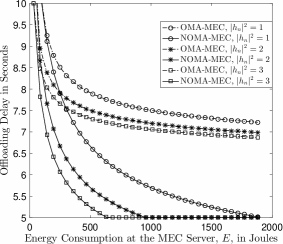
Figure 1: The impact of NOMA on MEC offloading delay. $N=15$ and $D_{m}=5$.

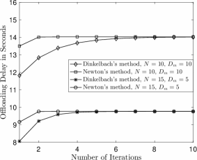
Figure 2: The convergence comparison between the two proposed iterative methods with $|h_{n}|^{2}=1$.

V Conclusions

In this paper, two iterative algorithms have been developed to minimize the offloading delay of NOMA-MEC. The optimality of the algorithms has been proven and their rates of convergence were also analyzed. Furthermore, criteria for choosing between the three possible modes, OMA, pure NOMA, and H-NOMA, for MEC offloading have been established.

References

• [1] Z. Ding, P. Fan, and H. V. Poor, “Impact of non-orthogonal multiple access on the offloading of mobile edge computing,” IEEE Trans. Commun., (submitted) Available on-line at arXiv:1804.06712.
• [2] F. Wang, J. Xu, and Z. Ding, “Optimized multiuser computation offloading with multi-antenna NOMA,” in Proc. IEEE Globecom Workshops, Singapore, Dec. 2017, pp. 1–6.
• [3] A. Kiani and N. Ansari, “Edge computing aware NOMA for 5G networks,” IEEE Internet of Things Journal, vol. PP, no. 99, pp. 1–1, 2018.
• [4] Z. Ding, J. Xu, O. A. Dobre, and H. V. Poor, “Joint power and time allocation for NOMA-MEC offloading,” IEEE Wireless Commun. Lett., (submitted) Available on-line at arXiv:1807.06306.
• [5] W. Dinkelbach, “On nonlinear fractional programming,” Management Science, vol. 13, no. 7, pp. 492 – 298, 1967.
• [6] S. Boyd and L. Vandenberghe, Convex optimization.   Cambridge University Press, Cambridge, UK, 2003.
• [7] E. Hildebrand, Introduction to Numerical Analysis.   Dover, New York, USA, 1987.