Taylor approximation to treat nonlocality in scattering process

Abstract

Study of scattering process in the nonlocal interaction framework leads to an integro-differential equation. The purpose of the present work is to develop an efficient approach to solve this integro-differential equation with high degree of precision. The method developed here employs Taylor approximation for the radial wave function which converts the integro-differential equation in to a readily solvable second-order homogeneous differential equation. This scheme is found to be computationally efficient by a factor of 10 when compared to the iterative scheme developed in J. Phys. G Nucl. Part. Phys. 45, 015106 (2018). The calculated observables for neutron scattering off ²⁴Mg, ⁴⁰Ca, ¹⁰⁰Mo and ²⁰⁸Pb with energies up to 10 MeV are found to be within at most 8$\%$ of those obtained with the iterative scheme. Further, we propose an improvement over the Taylor scheme that brings the observables so close to the results obtained by iterative scheme that they are visually indistinguishable. This is achieved without any appreciable change in the run time.

I Introduction

The nonlocal interaction framework finds its application in diverse range of scientific areas such as Physics and Quantum Biology Schweber (1961); Naumkin and Shishmarëv (1994); Cunha et al. (1996); Alfimov and Silin (1994); Mogilner and Edelstein-Keshet (1999); Wang and Wang (2016). In such studies, the dynamics of the system is modelled in terms of integro-differential equation, which is usually difficult to solve analytically or even numerically. Hence, one has to resort to efficient techniques that yield highly precise solutions.

In the domain of nuclear physics, the many-body nature of the nucleus makes it imperative to study processes such as scattering and reaction in the nonlocal interaction framework Lemere et al. (1979); Balantekin et al. (1998); Frahn (1956); Frahn and Lemmer (1957). As a consequence the conventional Schrödinger equation becomes an integro-differential equation, which is written as:

$$\left[\frac{\hbar^{2}}{2\mu}\nabla^{2}+U_{SO}{\bf L}\cdot{\boldsymbol{\sigma}}+E\right]\Psi({\bf r})=\int V({\bf r},{\bf r^{\prime}})\Psi({\bf r^{\prime}})d{\bf r^{\prime}}\,,$$ (1)

where $U_{SO}\,{\bf L}\cdot{\boldsymbol{\sigma}}$ is the local spin-orbit interaction, while $V({\bf r},{\bf r^{\prime}})$ is the nonlocal interaction kernel. Often this integro-differential equation is solved by using its Fourier transform in momentum space, which leads to a Fredholm integral equation of the second kind. This approach has been used to study scattering and bound states of nuclei Viviani et al. (2007); So et al. (2013).

Nevertheless, extensive studies in coordinate representation have been done to develop techniques that give precise solutions of Eq.(1) Frahn (1956); Frahn and Lemmer (1957); Perey and Buck (1962); S. Ali and Husain (1972); Ahmad et al. (1975); Rawitscher (2012). The most popular of them is the work of Perey and Buck Perey and Buck (1962) where the authors construct a local equivalent potential from the nonlocal nucleon-nucleus potential, which in turn is used to solve the integro-differential equation iteratively.

In our recent work Upadhyay et al. (2018), we have developed a readily implementable technique using the second mean value theorem (MVT) of the integral calculus Atkinson (2008) to solve the integro-differential equation. The advantage of the method is that it converts the integro-differential equation to the conventional Schrödinger equation. However, as shown in Upadhyay et al. (2018) to get a precise solution of Eq.(1), an iterative scheme has been employed which is initiated by solution to the homogeneous equation. The iterative scheme, thus developed, is found to be robust but is time consuming due to its slow convergence rate.

In this paper we develop a very efficient technique to solve Eq.(1) that yields results with precision comparable to those obtained by the full iterative MVT (IMVT) scheme of Ref. Upadhyay et al. (2018). For this purpose, we use Taylor approximation for the radial wave function which has been known for a long time, see for example Ref. Glendenning (1983). This method converts the integro-differential equation to a homogeneous second-order differential equation that can be easily solved. Further, to test the accuracy of the technique we have studied neutron scattering off different targets spanning the entire periodic table in the energy range up to 10 MeV.

The Taylor approximation approach developed to solve Eq.(1) forms the subject matter of Section-II. Results along with discussions are presented in Section-III, while the conclusions are given in Section-IV.

II Formalism

In order to study scattering of neutrons from the spin-zero nucleus, we start with partial wave expansion of Eq.(1). This is done by writing scattering wave function, $\Psi({\bf r})$, and the nonlocal interaction kernel, $V({\bf r},{\bf r^{\prime}})$ as:

$$\Psi({\bf r}) = \sum_{lm_{l}m_{s}}\frac{u_{jl}(r)}{r}\,\bigg{\langle}l\,\frac{1}{2}\,m_{l}\,m_{s}\,\bigg{|}\,j\,(m_{l}+m_{s})\bigg{\rangle}$$ (2)

$$\hskip 42.67912pt\times\,\,i^{l}\,Y_{lm_{l}}(\Omega_{r})\,\chi_{\frac{1}{2}m_{s}},$$

$$V({\bf r},{\bf r^{\prime}}) = \sum_{l}\frac{(2l+1)}{4\pi}\frac{g_{l}(r,r^{\prime})}{rr^{\prime}}\,P_{l}\left({\rm cos}\,\theta\right)\,,$$ (3)

with $\theta$ being the angle between ${\bf r}$ and ${\bf r^{\prime}}$ Perey and Buck (1962); Upadhyay et al. (2018).

The resulting radial equation is

$$\hskip 31.2982pt\hat{\mathcal{L}}\,u_{jl}(r)\,=\,\frac{2\mu}{\hbar^{2}}\int_{0}^{\infty}g_{l}(r,r^{\prime})u_{jl}(r^{\prime})dr^{\prime},$$ (4)

$${\rm where,}\,\,\hat{\mathcal{L}}\equiv\left[\frac{d^{2}}{dr^{2}}-\frac{l(l+1)}{r^{2}}+\frac{2\mu U_{SO}(r)}{\hbar^{2}}f_{jl}+\frac{2\mu\,E}{\hbar^{2}}\right]\,,$$

$$f_{jl}=\frac{1}{2}\left[j(j+1)-l(l+1)-\frac{3}{4}\right]\,\,\,{\rm with}\,\,j=l\pm 1/2\,,\,\,{\rm and}$$

$$g_{l}(r,r^{\prime})=2\pi rr^{\prime}\,\int_{-1}^{1}V\left({\bf r},{\bf r^{\prime}}\right)\,P_{l}\left({\rm cos}\,\theta\right)d\left({\rm cos}\,\theta\right)\,.$$ (5)

For the interaction kernel, $V\left({\bf r},{\bf r^{\prime}}\right)$, we use Frahn and Lemmer prescription Frahn (1956); Frahn and Lemmer (1957),

$$V({\bf r},{\bf r^{\prime}})=\frac{1}{\pi^{3/2}\beta^{3}}\,{\rm exp}\left[-\,\frac{\left|{\bf r}-{\bf r^{\prime}}\right|^{2}}{\beta^{2}}\right]U\left(\frac{\left|{\bf r}+{\bf r^{\prime}}\right|}{2}\right)\,,$$ (6)

where $\beta$ is the nonlocal range parameter. In this work, the energy and mass independent nucleon-nucleus potential, $U$, is taken to be of Wood-Saxon form. The parameters for this potential are taken from Tian et al. Tian et al. (2015). For further details regarding potential refer to Sec. 2.1 of Upadhyay et al. (2018). Following the convention adopted in Upadhyay et al. (2018), this potential will be referred to as ‘TPM15’.

To begin with, we enlist the salient features of the IMVT approach developed earlier in Upadhyay et al. (2018).

II.1 The IMVT Approach

In the IMVT approach, using the second mean value theorem of the integral calculus Atkinson (2008), the nonlocal interaction kernel is written as

$$\int_{0}^{\infty}g_{l}(r,r^{\prime})u_{jl}(r^{\prime})dr^{\prime}\,\approx\,u_{jl}(r)\int_{0}^{\infty}g_{l}(r,r^{\prime})dr^{\prime},$$ (7)

where the observation that $g_{l}(r,r^{\prime})$ is strongly peaked at $r$=$r^{\prime}$ is incorporated. Substituting this in Eq.(4), we obtain a homogeneous equation of the form

$$\hat{\mathcal{L}}\,u_{jl}(r)\,=\,\frac{2\mu U^{\rm eff}_{l}(r)}{\hbar^{2}}u_{jl}(r),$$ (8)

where the dominant effect of nonlocality is contained in the effective local potential, $\displaystyle{U^{\rm eff}_{l}(r)=\int_{0}^{\infty}g_{l}(r,r^{\prime})dr^{\prime}}$. Further, this potential is independent of energy but depends upon partial waves.

The solution of Eq.(4) is obtained by implementing an iterative scheme. This scheme is initiated by the solution to the above homogeneous equation (Eq.(8)) and the subsequent iterants are obtained by solving:

$$\hat{\mathcal{L}}u^{i+1}_{jl}(r) - \frac{2\mu\,U^{\rm eff}_{l}(r)}{\hbar^{2}}u^{i+1}_{jl}(r)$$

$$=\frac{2\mu}{\hbar^{2}}\int_{0}^{\infty}g_{l}(r,r^{\prime})u^{i}_{jl}(r^{\prime})\,dr^{\prime}-\frac{2\mu U^{\rm eff}_{l}(r)}{\hbar^{2}}u^{i}_{jl}(r)\,,$$

for all $i\geq 0$. The iterations are continued till the absolute value of difference between the logarithmic derivatives of the wave functions at the matching radius in the $i^{\rm th}$ and the $(i+1)^{\rm th}$ steps match within the desired precision, $\epsilon$.

The scattering wave function is obtained with the radial step size of 0.02 fm and matching radius of 20 fm. To obtain converged logarithmic derivative with $\epsilon\sim 10^{-6}$ at a given energy, the typical run time required is about an hour on a single Intel i7-6700 processor. Further, the run time scales almost linearly with the number of partial waves and energy, making the method time consuming. The fact that the IMVT scheme though robust, is time consuming, limits its usability to routine and large scale calculations.

To partially remedy this limitation, in Ref.Upadhyay et al. (2018) it was proposed that instead of full iterative procedure computation can be done with only one iteration. This results in speed-up of calculations by a factor of 4 as compared to the IMVT scheme. However, we would like to point out that the success of this solution depends strongly on the choice of nucleon-nucleus potential, mass of target as well as the projectile energy. For example, in case of neutron scattering off ²⁰⁸Pb and energies up to 2 MeV, it was found that the results for TPM15 potential with one iteration deviates from the IMVT results by as much as 20$\%$. Hence, it is important to develop a robust and efficient scheme to obtain precise solution to Eq.(4).

II.2 The Taylor Approximation Approach

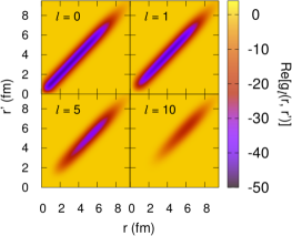
(a)  Real part

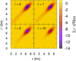
(b)  Imaginary part

Figure 1: Behavior of $g_{l}(r,r^{\prime})$ as a function of distance for different $l$. Calculations are done for neutron scattering off ²⁰⁸Pb using TPM15 potential Tian et al. (2015).

The principal objective of this work is to devise an efficient method to solve Eq.(4) with precision comparable to that obtained by the IMVT approach. To achieve this we examine the structure of nonlocal kernel, $g_{l}(r,r^{\prime})$, closely. As an illustration, in Fig. 1 we show the nonlocal kernel for neutron scattering off ²⁰⁸Pb using TPM15 potential Tian et al. (2015). As can be seen from the figure, the nonlocality is dominant around the line $r$=$r^{\prime}$. Any appreciable deviation from this line makes the contribution from the nonlocal kernel insignificant.

Motivated by this observation, we write $r^{\prime}$=$r+\Delta$ and expand the wave function $u_{jl}(r^{\prime})$ about $r$=$r^{\prime}$ using Taylor’s theorem Kline (1998) as

$$u_{jl}(r^{\prime})=P_{n}(r^{\prime})+R_{n}(r^{\prime})\,,\,\,\,\,(n\,\geq\,0)$$ (10)

where $P_{n}(r^{\prime})$ is the $n$-th order Taylor polynomial, written as

$$P_{n}(r^{\prime})=u_{jl}(r)+\sum_{\lambda=1}^{n}\frac{\Delta^{\lambda}}{\lambda!}\,\frac{d^{\lambda}u_{jl}(r)}{dr^{\lambda}}\,,$$ (11)

while the remainder term, $R_{n}(r^{\prime})$, is written as

$$R_{n}(r^{\prime})=\frac{\Delta^{n+1}}{(n+1)!}\,\frac{d^{n+1}u_{jl}(\xi)}{dr^{n+1}}\,,$$ (12)

for some $\xi$ between $r$ and $r^{\prime}$. Since the wave functions are guaranteed to be differentiable up to second-order for nonsingular potentials, we expand $P_{n}(r^{\prime})$ up to first-order ($n$=1) and retain the remainder term giving

$$u_{jl}(r^{\prime})=u_{jl}(r)+\Delta\,\frac{du_{jl}(r)}{dr}+\frac{\Delta^{2}}{2}\,\frac{d^{2}u_{jl}(\xi)}{dr^{2}}\,.$$ (13)

As the kernel is sharply peaked around $r$=$r^{\prime}$ (see Fig. 1), we take $\xi\approx r$. Thus, the integral on the right hand side of Eq.(4) can be written as:

$$\frac{2\mu}{\hbar^{2}}\int_{0}^{\infty}g_{l}(r,r^{\prime})u_{jl}(r^{\prime})dr^{\prime}=u_{jl}(r)I_{l0}(r)+\frac{du_{jl}(r)}{dr}I_{l1}(r)$$

$$\hskip 142.26378pt+\frac{d^{2}u_{jl}(r)}{dr^{2}}I_{l2}(r)$$ (14)

$$\hskip 5.69046pt{\rm where,}\,\,\,I_{ln}(r)=\frac{2\mu}{\hbar^{2}}\int_{0}^{\infty}\frac{\Delta^{n}}{n!}\,g_{l}(r,r^{\prime})dr^{\prime}\,,$$ (15)

with $0\leq n\leq 2$. Substituting this in Eq.(4) and rearranging the terms, we get a homogeneous second-order differential equation written as

$$\hat{\mathcal{O}}u_{jl}(r)=0\,,$$ (16)

where,

$$\hat{\mathcal{O}}\equiv\frac{d^{2}}{dr^{2}}-X_{l}(r)\frac{d}{dr}+W_{l}(r)\bigg{[}-\frac{l(l+1)}{r^{2}}\,\,\,\,\,\,\,$$ (17)

$$\hskip 56.9055pt+\,\frac{2\mu U_{SO}(r)}{\hbar^{2}}f_{jl}+\frac{2\mu\,E}{\hbar^{2}}-I_{l0}(r)\bigg{]}\,,$$

$$X_{l}(r)=\frac{I_{l1}(r)}{(1-I_{l2}(r))}\,\,\,{\rm and}\,\,\,W_{l}(r)=\frac{1}{(1-I_{l2}(r))}\,.$$ (18)

The obtained equation is a simple second order differential equation that can be readily solved. The first-order derivative appears explicitly in Eq.(16) and enough care has to be taken to evaluate it accurately. For this we revisit the behaviour of the wave function near the origin.

Near the origin, Eq.(16) becomes

$$\left[\frac{d^{2}}{dr^{2}}-\frac{l(l+1)}{r^{2}}+\frac{2\mu\,E}{\hbar^{2}}\right]u_{jl}(r)\,\approx\,0\,,\,\,\,\,\,\,\,\,(r\to 0)\,.$$ (19)

Redefining $\displaystyle{u_{jl}(r)\,=\,r^{l+1}\,\phi_{l}(r)}$, we get

$$\phi^{\prime\prime}_{l}(r)+\frac{2(l+1)}{r}\phi^{\prime}_{l}(r)+\frac{2\mu\,E}{\hbar^{2}}\phi_{l}(r)\,\approx\,0\,.$$ (20)

To solve the above differential equation, we use Frobenius method Simmons (2015) and obtain

$$\phi_{l}(r\to 0)\,=\,\sum_{\lambda=0}^{\infty}\frac{(-)^{l}\,(kr)^{2\lambda}}{2^{\lambda}\,\lambda!\,(2l+2\lambda+1)!!}\,\,.$$ (21)

Retaining the first four term of the series (up to $\lambda$=3), the expression for $u_{jl}(r)$ near origin is written as

$$u_{jl}(r\to 0)\,\approx\,\frac{r^{l+1}}{(2l+1)!!}\left[1-\frac{r^{2}k^{2}}{2(2l+3)}+\frac{r^{4}k^{4}}{8(2l+3)(2l+5)}-\frac{r^{6}k^{6}}{48(2l+3)(2l+5)(2l+7)}\right].$$ (22)

Now the first-order derivative appearing in Eq.(16) can be calculated accurately using Eq.(22). This expression also complies with the fact that $u_{j0}(0)$=0, $u^{\prime}_{j0}(0)$=1 for $l$=0 and $u_{jl}(0)$=$u^{\prime}_{jl}(0)$=0 for $l\neq$0. Finally, using Eq.(22) and its derivative as the initial conditions, we solve Eq.(16) using the fourth order Runge-Kutta method Hairer et al. (2008).

III Results

III.1 The Taylor Approximation Approach

To illustrate the method developed above, we consider neutron scattering off ²⁴Mg, ⁴⁰Ca, ¹⁰⁰Mo and ²⁰⁸Pb with energies up to 10 MeV. Calculations are done with TPM15 potential Tian et al. (2015). Similar to the IMVT calculations, the radial step size is taken to be 0.02 fm, while the matching radius is assumed to be 20 fm.

In order to test the accuracy of the Taylor scheme, in Fig. 2 we compare the results of the present work (labeled as Taylor) with those obtained by the IMVT scheme (labeled as IMVT) along with the data Bommer et al. (1976); Fowler et al. (1973); Finlay et al. (1993); Divadeenam et al. (1968); Pasechnik et al. (1980); Harvey (1999). The cross sections calculated using the Taylor scheme are found to be close to those obtained by the IMVT scheme. Further, both the calculated results are in good agreement with the experiments.

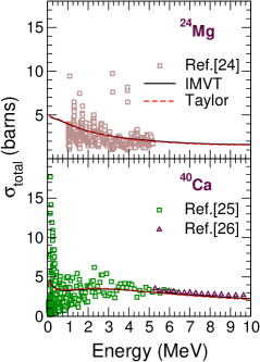
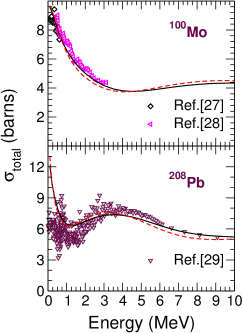
Figure 2: Calculated total cross sections for neutron scattering off ²⁴Mg, ⁴⁰Ca, ¹⁰⁰Mo and ²⁰⁸Pb along with the data Bommer et al. (1976); Fowler et al. (1973); Finlay et al. (1993); Divadeenam et al. (1968); Pasechnik et al. (1980); Harvey (1999). The Taylor results are shown by the dashed red line while the IMVT results Upadhyay et al. (2018) are shown by the solid black line. Calculations are done using TPM15 potential Tian et al. (2015).

At a finer level, the Taylor and the IMVT results slightly differ from each other. This difference can be quantified by studying the behavior of $\delta(E)$, defined as

$$\delta(E)\,=\,\frac{\sigma_{\rm IMVT}(E)-\sigma_{\rm Taylor}(E)}{\sigma_{\rm IMVT}(E)}\times 100$$ (23)

with respect to neutron energy, $E$. In Fig. 3 we plot the quantity $\delta(E)$ as a function of energy for all the targets. It is seen that the cross sections obtained by the Taylor scheme are within at the most 8$\%$ of those obtained by the IMVT scheme for all the cases.

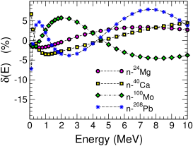
Figure 3: Quantity $\delta(E)$ as a function of energy, $E$, for neutron scattering off different nuclei.

The typical run time required for the Taylor scheme is about 5 minutes for a given energy on a single Intel i7-6700 processor. This demonstrates that the Taylor scheme is computationally efficient by a factor of 10 in comparison to IMVT approach and at the same time yields results within 8$\%$ of the IMVT results, which is gratifying.

III.2 Iterative Perturbation Approach

The Taylor scheme devised in the previous section can be improved further without any appreciable change in the run time. This is achieved by solving Eq.(4) using an Iterative Perturbation approach (IPA). In this approach, the exact solution is expressed as a perturbation series

$$u_{jl}(r)\,=\,u_{jl}^{0}(r)\,+\,\sum_{k=1}^{\infty}u_{jl}^{k}(r)\,,$$ (24)

where $u_{jl}^{0}(r)$ is the solution of Eq.(16) and $u_{jl}^{k}(r)$ is the higher-order correction that quantifies the deviation from the exact solution. These higher-order corrections are obtained with the help of following iterative scheme:

$$\hat{\mathcal{O}}u_{jl}^{i+1}(r)-W_{l}(r)\,\xi_{jl}^{i}(r)\,=0\,,$$ (25)

where,

$$\xi_{jl}^{i}(r)\,=\,\frac{2\mu}{\hbar^{2}}\int_{0}^{\infty}g_{l}(r,r^{\prime})u_{jl}^{i}(r^{\prime})dr^{\prime}\,-\,\hat{\mathcal{G}}\,u_{jl}^{i}(r)\,,$$ (26)

where $i\geq 0$ and $\displaystyle{\hat{\mathcal{G}}\,\equiv\,I_{l0}(r)+I_{l1}(r)\frac{d}{dr}+I_{l2}(r)\frac{d^{2}}{dr^{2}}}$. The corrected wave function, $u_{jl}(r)$, thus obtained, is then matched with the free state wave function to calculate the $S$-matrix, which in turn is employed in computation of observables.

In Fig. 4 we quantify the accuracy of IPA cross sections calculated after 5 iterations (referred as IPA5) relative to the IMVT cross sections by plotting $\delta(E)$ as a function of energy. The IPA5 cross sections are found to be within 2$\%$ of the IMVT cross sections at all energies for all the cases.

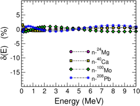
Figure 4: Same as Fig 3, but $\delta(E)$ computed for IPA5 relative to IMVT.

Further, in Fig. 5 we show the total cross sections calculated by IPA5 for neutron scattering off different nuclei along with the data Bommer et al. (1976); Fowler et al. (1973); Finlay et al. (1993); Divadeenam et al. (1968); Pasechnik et al. (1980); Harvey (1999). Visually, the IPA5 and the IMVT results are indistinguishable. Computationally there is no significant change at all in the run time when compared with that required for the Taylor scheme.

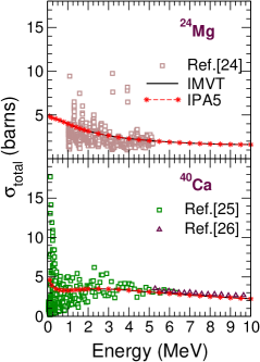
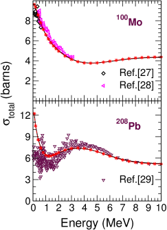
Figure 5: Same as Fig 2, but for IPA5. The IPA5 results are shown by the starred red line.

These results demonstrate that the improved technique IPA yields highly precise solution to Eq.(4). Further, the technique is highly efficient since we have achieved a speed-up by a factor of 10 as compared to the IMVT scheme, which is extremely significant in particular when it comes to large scale computations.

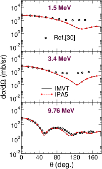
(a)  n-²⁴Mg scattering

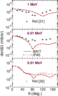
(b)  n-⁴⁰Ca scattering

Figure 6: Calculated angular distributions for neutron scattering off ²⁴Mg and ⁴⁰Ca along with the data Th.Schweitzer et al. (1978); Toepke (1974); Tornow et al. (1982). The IPA5 results are shown by the starred red line while the IMVT results Upadhyay et al. (2018) are shown by the solid black line. Calculations are done using TPM15 potential Tian et al. (2015).

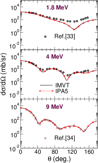
(a)  n-¹⁰⁰Mo scattering

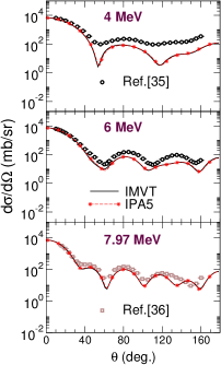
(b)  n-²⁰⁸Pb scattering

Figure 7: Same as Fig. 6, but for neutron scattering off ¹⁰⁰Mo and ²⁰⁸Pb along with the data Smith et al. (1975); Rapaport et al. (1979); Annand et al. (1985); Roberts et al. (1991).

III.3 Angular Distributions

For completeness, in Figs. 6-7 we show various calculated angular distributions along with the experimental data Th.Schweitzer et al. (1978); Toepke (1974); Tornow et al. (1982); Smith et al. (1975); Rapaport et al. (1979); Annand et al. (1985); Roberts et al. (1991). As observed earlier, again the IPA5 and the IMVT results are found to be indistinguishable. For ²⁴Mg and ⁴⁰Ca we observe that the calculated results are reasonably consistent with the data at low energies, while those for ¹⁰⁰Mo and ²⁰⁸Pb are in good accord at all the energies. It may be mentioned that the parameters for TPM15 potential are obtained by fitting the nucleon scattering data on nuclei ranging from ²⁷Al to ²⁰⁸Pb with incident energies around 10 MeV to 30 MeV. Probably a better agreement can be achieved with more appropriate choice of potential. Further investigations along these lines are in progress.

III.4 Robustness of IPA

In the present work, a separable form for the interaction kernel (see Eq.(6)) is used, which is given as

$$V({\bf r},{\bf r^{\prime}})=H\left(\left|{\bf r}-{\bf r^{\prime}}\right|\right)U\left(\frac{\left|{\bf r}+{\bf r^{\prime}}\right|}{2}\right)\,.$$ (27)

The function $H\left(\left|{\bf r}-{\bf r^{\prime}}\right|\right)$ is chosen to be a Gaussian with the range $\beta$=0.9 fm (as given in Tian et al. (2015)) and is normalized to unity. To establish the robustness of IPA, it is essential to study its sensitivity to different forms of nonlocality.

III.4.1 Impact of different forms of nonlocality

As a first step, we explore the impact of different forms of $H\left(\left|{\bf r}-{\bf r^{\prime}}\right|\right)$ with same normalization and rms radius but different shapes. For this we consider an exponential function:

$$H\left(\left|{\bf r}-{\bf r^{\prime}}\right|\right)\,=\,\frac{1}{8\pi\alpha^{3}}\,{\rm exp}\left(-\frac{|\bf{r}-\bf{r^{\prime}}|}{\alpha}\right)\,.$$ (28)

which is normalized similar to the Gaussian function. Further, the nonlocal range $\alpha$ has been chosen in such a way that both the Gaussian and exponential form factors have the same rms radii, giving: $\alpha\,=\,\beta/\sqrt{8}$.

In Fig. 8 we show the total cross sections calculated by using Gaussian and exponential forms of nonlocality in IPA5 calculations for neutron scattering off different nuclei. As expected, different forms for $H\left(\left|{\bf r}-{\bf r^{\prime}}\right|\right)$ having same normalization and rms radius give similar results Upadhyay et al. (2018).

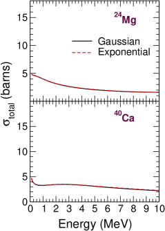
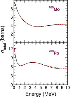
Figure 8: Calculated total cross sections for neutron scattering off ²⁴Mg, ⁴⁰Ca, ¹⁰⁰Mo and ²⁰⁸Pb. The results for Gaussian form of nonlocality are shown by the solid black line while the results for exponential form are shown by the dashed red line. Calculations are done by IPA5 using TPM15 potential Tian et al. (2015). For exponential form, $\alpha$=0.318 fm.

III.4.2 Impact of different ranges of nonlocality

Next we explore the impact of different rms radius on Gaussian form of nonlocality. For this we consider different values of $\beta$, namely, 0.6 fm, 0.9 fm and 1.2 fm in TPM15 potential Tian et al. (2015) and calculate total cross sections using 5 iterations of IPA (IPA5). As an illustration, in Fig. 9 we show the calculated cross sections for neutron scattering off ²⁰⁸Pb. The cross sections are found to be extremely sensitive to $\beta$. However, it should be noted that $\beta$ is an additional parameter in TPM15 potential. Hence, in principle, any change in $\beta$ should be accompanied by refitting of the potential parameters Perey and Buck (1962). Nevertheless, this study illustrates the numerical robustness of IPA against the range of nonlocality.

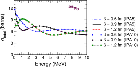
Figure 9: Calculated total cross sections for neutron scattering off ²⁰⁸Pb. Calculations are done using Gaussian form of nonlocality and TPM15 potential Tian et al. (2015) for different values of $\beta$.

In order to test the convergence properties of IPA, in Fig. 9 we also show the calculated cross sections with 10 iterations of IPA (labeled as IPA10) for different values of $\beta$. As can be seen, irrespective of $\beta$ value, convergence is achieved with 5 iterations. Further, we would like to point out that the runtime required for IPA10 is only marginally longer than that for IPA5.

Thus, it can be concluded that IPA is a robust technique and its validity seems to be independent of the choice of nonlocal form factor.

IV Summary and Conclusion

A very efficient and highly precise technique to solve the integro-differential equation appearing in scattering problem is developed. It is achieved by employing Taylor approximation to the radial wave function. This scheme transforms the integro-differential equation to a second-order homogeneous differential equation which can be solved easily.

The observables obtained by the Taylor scheme for neutrons scattering off ²⁴Mg, ⁴⁰Ca, ¹⁰⁰Mo and ²⁰⁸Pb are found to be within 8$\%$ of those obtained by the IMVT scheme at all the projectile energies. We have demonstrated that the precision of solution can be improved further by using the “Iterative Perturbative Approach”, which calculates the successive corrections to the solution obtained by using the Taylor scheme. With just 5 iterations of IPA the observables for all the cases and at all the energies are found to be within 2$\%$ of those obtained by the IMVT scheme without any appreciable change in the run time. Further, the calculated observables are in accord with the experiments for all the cases.

The technique developed here is found to be robust and numerically stable. This conclusion seems to be independent of the choice of the form of nonlocality. Therefore, it is expected to be useful in diverse areas of science where existence of nonlocality leads to an integro-differential equation.