CosmicGrowth Simulations—Cosmological simulations for structure growth studies

Abstract

I present a large set of high resolution simulations, called CosmicGrowth Simulations, which were generated with either 8.6 billion or 29 billion particles. As the nominal cosmological model that can match nearly all observations on cosmological scales, I have adopted a flat Cold Dark Matter (CDM) model with a cosmological constant $\Lambda$ ($\Lambda{\rm CDM}$). The model parameters have been taken either from the latest result of the WMAP satellite (WMAP $\Lambda{\rm CDM}$) or from the first year’s result of the Planck satellite (Planck $\Lambda{\rm CDM}$). Six simulations are produced in the $\Lambda{\rm CDM}$ models with two in the Planck model and the others in the WMAP model. In order for studying the nonlinear evolution of the clustering, four simulations were also produced with $8.6$ billion particles for the scale-free models of an initial power spectrum $P(k)\propto k^{n}$ with $n=0$,$-1$,$-1.5$ or $-2.0$. Furthermore, two radical CDM models (XCDM) are simulated with 8.6 billion particles each. Since the XCDM have some of the model parameters distinct from those of the $\Lambda{\rm CDM}$ models, they must be unable to match the observations, but are very useful for studying how the clustering properties depend on the model parameters. The Friends-of-Friends (FoF) halos were identified for each snapshot and subhalos were produced by the Hierarchical Branch Tracing (HBT) algorithm. These simulations form a powerful database to study the growth and evolution of the cosmic structures both in theories and in observations.

Received January 1, 2016; accepted January 1, 2016; published online January 1, 2016

galaxy formation, structure formation in the Universe, cosmology

1 Introduction

In the past forty years N-body simulations have played a key role in advancing our knowledge about structure formation in the Universe([1, 2] for recent reviews). Perturbation theories have been tested, refined and calibrated with N-body simulations [3, 4]. The clustering and abundance of dark matter halos has been found to have discrepancies with the Press-Schechter theory [5, 6], which promoted massive studies on the subject[7, 8]. Now the halo bias, including its dependence on the halo assembly history[9], has been understood reasonably well[10]. The density profile of halos has been found to be well described by the Navarro, Frenk and White form[11]. Furthermore, the internal structures are found to rely on their mass growth[12, 13], both of which can be accurately described by simple scaling forms[14, 15]. The halos have been found to be triaxial, and the shape distributions are accurately given in simple scaling forms[16]. The subhalo abundance in each halo is approximately universal once the subhalo mass is scaled by the host halo mass[17, 18]. All these results have formed important ingredients for understanding how the cosmic structures have developed. They are also the bases from which galaxy formation theories are constructed and confronted with various observations. N-body simulations are widely used to plant galaxies, through so-called semi-analytical modeling[19, 20, 21, 22], to form model galaxy catalogs that are used to understand various aspects of galaxy formation, and are directly compared with observations of galaxies. N-body simulations are also used to empirically derive the occupation distributions, e.g. the luminosity function and the mass function of certain type galaxies in dark matter halos, from large galaxy surveys through adopting methods, such as a Halo Occupation Distribution (HOD)[23, 24], Conditional Luminosity Function[25], or Abundance Matching[26, 27, 28].

With the development of large galaxy surveys in the near future, the properties of the dark energy, test of General Relativity, and the formation and evolution of galaxies will become the focuses of the future research. These studies have raised new demands for N-body simulations. For example, for studying the dark energy and testing gravity models, weak lensing and redshift distortion are two important observables. However, to extract the physical information from the observations, one has to take into account of all non-linear effects, such as non-linear evolution of cosmic structures, spatial and velocity biases of galaxies, intrinsic alignments of galaxies, real space to redshift space mapping. This means that N-body simulations have to well resolve galaxies, while they have to have a volume sufficiently large to cover large scale structures in the Universe.

In this paper, I present a new set of N-body cosmological simulations called CosmicGrowth simulations. Since the simulations have been designed mainly for studying the acceleration of the cosmic expansion and for studying the clustering of dark matter and galaxies, I have generated simulations not only for ${\Lambda}$CDM (cosmological constant $\Lambda$ plus Cold Dark Matter) models, but also for the scale-free (SF) models and other CDM like models (XCDM) that have the model parameters that are distinctly different from the observed ones. The main reason for producing SF and XCDM simulations is that they help us understand the nonlinear processes, formation of galaxies, and the effects of the cosmological parameters. This also manifests the uniqueness of our simulations that are distinct from those of other groups who usually only do $\Lambda$CDM simulations. As was shown by [6, 15], the SF simulations are very powerful for understanding the gravitational processes in forming cosmic structures, including large scale structures and internal structures of dark matter halos.

The paper is arranged as the following. In sect 2, I will describe the simulations, including how the catalogs of the dark matter halos and subhalos are constructed. Then in sect 3, I present the mass functions of dark matter halos in a typical $\Lambda$CDM model, to demonstrate the convergence of the halo catalog in different simulations. Our main conclusions will be summarized in sect 4

2 Simulations

2.1 Models

I choose the cosmological parameters compatible with the WMAP observations. I assume the universe is flat, with the current cosmic density contributed by the vacuum energy (or equivalently the cosmological constant) $\Omega_{\Lambda}$, by cold dark matter $\Omega_{\rm c}$ and by baryonic matter $\Omega_{b}$, where $\Omega_{x}$ is the density parameter, i.e. the density of the corresponding component $x$ in units of the critical density of the Universe at the current epoch. The primordial fluctuation is a Gaussian one with a power-law spectrum $\propto k^{n_{s}}$, and its amplitude is set by the rms linear density fluctuation $\sigma_{8}$ in a sphere of radius $8\,h^{-1}{\rm{Mpc}}$ at the current epoch, where $h$ is the Hubble constant in terms of $100{\rm\ kms^{-1}Mpc^{-1}}$ . In addition to the cosmic background radiation, there are three species of massless neutrinos in the Universe. I choose the cosmological model parameters as listed in Table 1, which are well consistent with the Seven-Year data and Nine-Year data of WMAP [29, 30]. I call this model as the WMAP cosmology.

After I had started the simulations, the Planck team released their observational results that yield new constraints on the cosmological parameters. While their results are consistent with those of the WMAP at 2$\sigma$ level, I generate simulations for the cosmological model set by their first year’s data[31], in order to study how the change of the parameters will impact on the structure formation . The cosmological parameters are listed in Table 1 with a label Planck.

While there is consensus that the $\Lambda$CDM models with the parameters taken above are the best-fitting models to the observations, it is known that there exist resolution problems in any simulation that may cause difficulties in interpretation of the simulation results especially on small or on the largest scales. The SF simulations, because of its scaling properties by construction, may help one understand the simulation limitations[32]. Also because of its scaling properties, it helps understanding the universal properties of clustering, such as the non-linear clustering, and the assembly, structures and clustering of dark matter halos. It also helps improving theoretical understanding of the halo formation, such as the seminal (Extended) Press-Schechter theories. I believe that the scale-free simulations will continue to play an important role in understanding the weak lensing and redshift space distortion in the era of studying the cosmic expansion. Therefore I have constructed SF simulations for $n=0$, $-1$, $-1.5$, and $-2$ respectively (Table 2). Why I have chosen to run more simulations around $n=-1.5$, because they have the slope similar to that of $\Lambda$CDM at the critical scale where the clustering become non-linear after redshift $z=3$. The initial condition is set in the same way as [6], i.e. the initial power spectrum at the particle Nyquist wavelength is $A/N_{p}$, where $N_{p}$ is the particle number in the simulation and $A$ is listed Table 2. As demonstrated in [6], in the case of $n=-2$, the fluctuation is quite nonlinear even at the start of the simulation. I actually generate the initial condition for $n=-2$ at $a=a_{i}/10$ with the fluctuation amplitude set to $A/100$, and evolve the initial condition by the PM version to $a_{i}$.

I also choose two CDM-like cosmological models that have model parameters strongly different that of the WMAP $\Lambda$CDM model. I call them as the $X$CDM models (Table 3). The $X$CDM1 has the same linear power spectrum as the WMAP $\Lambda{\rm CDM}$, but the universe is made of CDM only with $\Omega_{c}=1$. The $X$CDM2 has the same density parameters as the $X$CDM1 model, but its primordial power spectrum has $n_{s}=1$ and the transfer function is adopted from Barden et al. (BBKS)[33] with $\Omega_{c}h=0.5$. While we know these models do not fit the real Universe well, because of the change of the model parameters, they may help us understand how the properties of the structure growth will change with the parameters.

Table 1: The model parameters of $\Lambda{\rm CDM}$ simulations

Model	$\Omega_{b}$	$\Omega_{c}$	$\Omega_{\Lambda}$	$h$	$n_{s}$	$\sigma_{8}$
Planck $\Lambda{\rm CDM}$	$0.0487$	$0.2663$	$0.685$	$0.673$	$0.9603$	$0.829$
WMAP $\Lambda{\rm CDM}$	$0.0445$	$0.2235$	$0.732$	$0.71$	$0.968$	$0.83$

Table 2: The model parameters of the SF simulations

Model	$\Omega_{c}$	$\Omega_{\Lambda}$	$n$	$A$
SFn0	$1$	$0$	$0$	$0.7314$
SFn-1	$1$	$0$	$-1$	$0.5629$
SFn-1p5	$1$	$0$	$-1.5$	$0.4891$
SFn-2	$1$	$0$	$-2.0$	$0.4241$

Table 3: The model parameters of the XCDM simulations

Model	$\Omega_{b}$	$\Omega_{c}$	$\Omega_{\Lambda}$	$n_{s}$	$\sigma_{8}$	linear $P(k)$
XCDM1	$0.0$	$1.0$	$0$	$0.968$	$0.83$	WMAP $\Lambda{\rm CDM}$
XCDM2	$0.0$	$1.0$	$0$	$1.0$	$0.83$	BBKS

2.2 Simulation Parameters

For $\Lambda$CDM and $X$CDM models, I choose an initial redshift $z_{i}$ at which the simulation starts. The simulations are evolved with my adaptive parallel ${\rm P^{3}M}$ N-body code. The force between the particles is softened at small scale. The S2 form of Efstathiou et al [34] is taken, with the softening parameter $\eta$ being the scale beyond which the force between two particles is exact. This parameter is a key one that determines the simulation resolution at small scale. It also sets a constraint on the time step. Here I choose a constant time step $da$ in the universe scale factor $a$. Guided by our previous simulations, I set $\eta$, $da$ (and hence $N_{step}$) as listed in Table 4 and Table 6 for $\Lambda{\rm CDM}$ and $X$CDM simulations respectively. The scale factor $a$ is normalized to $a_{i}=1$ at $z_{i}$, and the box size $L$ and the softening length $\eta$ are in unit of $\,h^{-1}{\rm{Mpc}}$. In order to identify subhalos and form merger histories, I have output a large number of snapshots $N_{\rm snap}$ with an equal logarithmic interval in the scale factor $a$ from $z_{\rm out,1}$ to $z=0$.

Following [32], I take the time variable $p=a^{\frac{3}{n+3}}$ for the SF model with index $n$. The $\eta$ parameter is in units of the box size $L$. I evolve the the simulation to an epoch when the rms density fluctuation of a sphere of radius $R=0.05L$ becomes non-linear according to the linear perturbation theory. The simulation parameters are listed in Table 5. I start the simulation at $p_{i}=1$, and output the snapshots from $p_{out,1}$ in an equal logarithmic interval of $p$. The meaning of the other simulation parameters are the same as those for the $\Lambda{\rm CDM}$ models.

For XCDM models, I take the same simulation parameters as I did for WMAP_2048_1200 or Planck_2048_1200 (see Table 6).

Table 4: The $\Lambda{\rm CDM}$ simulations and the simulation parameters

Name	model	$N_{p}$	$L$	$da$	$\eta$	$z_{i}$	$N_{step}$	$z_{out,1}$	$N_{snap}$	realizations
Planck_2048_400	Planck $\Lambda{\rm CDM}$	$2048^{3}$	$400$	$0.0288$	$0.007$	$144$	$5000$	$16.87$	$100$	1
Planck_2048_1200	Planck $\Lambda{\rm CDM}$	$2048^{3}$	$1200$	$0.06$	$0.03$	$72$	$1200$	$7.30$	$24$	1
WMAP_2048_400	Planck $\Lambda{\rm CDM}$	$2048^{3}$	$400$	$0.0288$	$0.007$	$144$	$5000$	$16.87$	$100$	1
WMAP_2048_1200	Planck $\Lambda{\rm CDM}$	$2048^{3}$	$1200$	$0.06$	$0.03$	$72$	$1200$	$7.30$	$24$	1
WMAP_3072_600	Planck $\Lambda{\rm CDM}$	$3072^{3}$	$600$	$0.0288$	$0.01$	$144$	$5000$	$16.87$	$100$	3
WMAP_3072_1200	Planck $\Lambda{\rm CDM}$	$3072^{3}$	$1200$	$0.0288$	$0.02$	$144$	$5000$	$16.87$	$100$	1

Table 5: The SF simulations and the simulation parameters

Name	model	$N_{p}$	$dp$	$\eta$	$z_{i}$	$N_{step}$	$p_{out,1}$	$N_{snap}$	realizations
SFn0_2048	SFn0	$2048^{3}$	$0.0202$	$0.125\times 10^{-4}$	$1029.15$	$5000$	$2.37$	$50$	2
SFn-1_2048	SFn-1	$2048^{3}$	$0.0302$	$0.125\times 10^{-4}$	$151.00$	$5000$	$3.54$	$50$	2
SFn-1p5_2048	SFn-1p5	$2048^{3}$	$0.0401$	$0.125\times 10^{-4}$	$52.51$	$5000$	$4.69$	$50$	2
SFn-2_2048	SFn-2	$2048^{3}$	$0.0602$	$0.125\times 10^{-4}$	$16.38$	$5000$	$7.02$	$50$	1

Table 6: The XCDM simulations and the simulation parameters

Name	model	$N_{p}$	$L$	$da$	$\eta$	$z_{i}$	$N_{step}$	$z_{out,1}$	$N_{snap}$	realizations
XCDM1_2048_1200	XCDM1	$2048^{3}$	$1200$	$0.06$	$0.03$	$72$	$1200$	$7.30$	$24$	1
XCDM2_2048_1200	XCDM2	$2048^{3}$	$1200$	$0.06$	$0.03$	$72$	$1200$	$7.30$	$24$	1

2.3 FoF Groups, halos, and subhalos

Groups are identified with the Friends-of-Friends (FoF) algorithm with the linking length taken to be 0.2 times of the mean particle separation, and a FoF group catalog is constructed for each snapshot. It is known that some of the member particles in a FoF group are not bound, and the fraction of unbound particles increases with the decrease of the group mass. Following the practice of [35], I have removed all unbound particles from the FoF groups, and form a bound halo catalog for each snapshot. As one will see in the next section, the mass function of the halos converges well at the halo mass equivalent to $\sim 10$ times of the particle mass, while the effect of the unbound particles can be seen clearly for original FoF groups even at halo mass equivalent to 100 times of particle mass[35]. Therefore, I recommend to use the bound halo catalogs for future statistical studies.

Halos falling into a more massive halo will become subhalos. Subhalos are interesting structures, because they are the hosts of satellite galaxies in groups or clusters of galaxies. They also form potential wells to confine gas and to support the motion of the stars inside. The Hierarchical Branch Tracing (HBT) code[36] has been used to construct the merger tree and the subhalo catalogs.

3 Mass Functions of Dark Matter Halos

In Figure 1, I present the mass functions of the bound FoF halos in the WMAP cosmology at z=0. The red dots are for the simulation WMAP_3072_1200, and the blue and red lines are respectively for two realizations of the simulation WMAP_3072_600. I have plotted the mass functions above the halo mass corresponding to 10 particles. Since WMAP_3072_600 has resolutions 8 times better in mass and 2 times better in force than WMAP_3072_1200, it is amazing to see that mass functions agree nearly perfectly at the mass $5\times 10^{10}{\rm M_{\odot}}h^{-1}$ which corresponds to the mass of 13 particles in WMAP_3072_1200. Furthermore, one can see the mass functions of the two realizations of WMAP_3072_600 perfectly agree on the whole mass range except for the very massive end where fluctuations are expected for different realizations. The plot indicates that our procedure to remove the unbound particles in the FoF groups are very successful, and the bound group catalogs may be used for statistical analyses for the halo members above $\sim 13$.

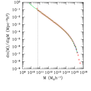
Figure 1: The mass functions of the halos in WMAP_3072_1200 (red dots) and in two realizations (blue and green lines respectively) of WMAP_3072_600.

4 Discussion and conclusions

I present a large set of high resolution simulations which were generated with either 8.6 billion or 29 billion particles. As for the nominal cosmological model that can match nearly all observations on cosmological scales, I have adopted a flat Cold Dark Matter (CDM) model with a cosmological constant $\Lambda$ ($\Lambda{\rm CDM}$). The model parameters have been taken either from the latest result of the WMAP satellite (WMAP $\Lambda{\rm CDM}$) or from the first year’s result of the Planck satellite (Planck $\Lambda{\rm CDM}$). Six simulations are produced in the $\Lambda{\rm CDM}$ models with two in the Planck model and the others in the WMAP model. In order for studying the nonlinear evolution of the clustering, four simulations were also produced with $8.6$ billion particles for the scale-free models of an initial power spectrum $P(k)\propto k^{n}$ with $n=0$,$-1$,$-1.5$ or $-2.0$. Furthermore, two radical CDM models (XCDM) are simulated with 8.6 billion particles each. Since XCDM models have some of the model parameters distinct from those of the $\Lambda{\rm CDM}$ models, they must be unable to match the observations, but are very useful for studying how the clustering properties depend on the model parameters. The Friends-of-Friends (FoF) halos were identified for each snapshot and subhalos were produced by the Hierarchical Branch Tracing (HBT) algorithm. I have demonstrated that the halos are well resolved and identified at a mass above that of 13 particles. These simulations form a powerful database to study the growth and evolution of the cosmic structures both in theories and in observations.

The work is supported by the NSFC (11320101002, 11533006, & 11621303) and 973 Program No. 2015CB857003. I am very grateful to Jiaxin Han for identifying subhalos for the $\Lambda$CDM simulations.

References

- [1] Frenk, C. S. and S. D. M. White, Annalen der Physik, 524,507 (2012)
- [2] Baugh, C. M., Publications of the Astronomical Society of Australia, 30,e030 (2013)
- [3] Takahashi, R., M. Sato, T. Nishimichi, A. Taruya, and M. Oguri, The Astrophysical Journal, 761,152 (2012)
- [4] Chen, J., P. Zhang, Y. Zheng, Y. Yu, and Y. Jing, The Astrophysical Journal, 861,58 (2018)
- [5] Jing, Y. P., The Astrophysical Journal, 515,L45 (1999)
- [6] Jing, Y. P., The Astrophysical Journal, 503,L9 (1998)
- [7] Sheth, R. K., H. J. Mo, and G. Tormen, Monthly Notices of the Royal Astronomical Society, 323,1 (2001)
- [8] Sheth, R. K. and G. Tormen, Monthly Notices of the Royal Astronomical Society, 308,119 (1999)
- [9] Gao, L., V. Springel, and S. D. M. White, Monthly Notices of the Royal Astronomical Society, 363,L66 (2005)
- [10] Han, J., Y. Li, Y. Jing, T. Nishimichi, W. Wang, and C. Jiang, ArXiv e-prints, arXiv:1802.09177 (2018)
- [11] Navarro, J. F., C. S. Frenk, and S. D. M. White, The Astrophysical Journal, 490,493 (1997)
- [12] Wechsler, R. H., J. S. Bullock, J. R. Primack, A. V. Kravtsov, and A. Dekel, The Astrophysical Journal, 568,52 (2002)
- [13] Zhao, D. H., H. J. Mo, Y. P. Jing, and G. Börner, Monthly Notices of the Royal Astronomical Society, 339,12 (2003)
- [14] Zhao, D. H., Y. P. Jing, H. J. Mo, and G. Börner, The Astrophysical Journal, 597,L9 (2003)
- [15] Zhao, D. H., Y. P. Jing, H. J. Mo, and G. Börner, The Astrophysical Journal, 707,354 (2009)
- [16] Jing, Y. P. and Y. Suto, The Astrophysical Journal, 574,538 (2002)
- [17] Gao, L., S. D. M. White, A. Jenkins, F. Stoehr, and V. Springel, Monthly Notices of the Royal Astronomical Society, 355,819 (2004)
- [18] Han, J., S. Cole, C. S. Frenk, and Y. Jing, Monthly Notices of the Royal Astronomical Society, 457,1208 (2016)
- [19] White, S. D. M. and C. S. Frenk, The Astrophysical Journal, 379,52 (1991)
- [20] Kauffmann, G., S. D. M. White, and B. Guiderdoni, Monthly Notices of the Royal Astronomical Society, 264,201 (1993)
- [21] Cole, S., A. Aragon-Salamanca, C. S. Frenk, J. F. Navarro, and S. E. Zepf, Monthly Notices of the Royal Astronomical Society, 271,781 (1994)
- [22] Kang, X., Y. P. Jing, H. J. Mo, and G. Börner, The Astrophysical Journal, 631,21 (2005)
- [23] Jing, Y. P., H. J. Mo, and G. Börner, The Astrophysical Journal, 494,1 (1998)
- [24] Berlind, A. A. and D. H. Weinberg, The Astrophysical Journal, 575,587 (2002)
- [25] Yang, X., H. J. Mo, and F. C. van den Bosch, Monthly Notices of the Royal Astronomical Society, 339,1057 (2003)
- [26] Rodríguez-Puebla, A., J. R. Primack, V. Avila-Reese, and S. M. Faber, Monthly Notices of the Royal Astronomical Society, 470,651 (2017)
- [27] Zu, Y. and R. Mandelbaum, Monthly Notices of the Royal Astronomical Society, 476,1637 (2018)
- [28] Xu, H., Z. Zheng, H. Guo, Y. Zu, I. Zehavi, and D. H. Weinberg, ArXiv e-prints, arXiv:1801.07272 (2018)
- [29] Hinshaw, G., and 20 colleagues, The Astrophysical Journal Supplement Series, 208,19 (2013)
- [30] Komatsu, E., and 20 colleagues, The Astrophysical Journal Supplement Series, 192,18 (2011)
- [31] Planck Collaboration, and 264 colleagues, Astronomy and Astrophysics, 571,A16 (2014)
- [32] Efstathiou, G., C. S. Frenk, S. D. M. White, and M. Davis, Monthly Notices of the Royal Astronomical Society, 235,715 (1988)
- [33] Bardeen, J. M., J. R. Bond, N. Kaiser, and A. S. Szalay, The Astrophysical Journal, 304,15 (1986)
- [34] Efstathiou, G., M. Davis, S. D. M. White, and C. S. Frenk, The Astrophysical Journal Supplement Series, 57,241 (1985)
- [35] Jing, Y. P., Y. Suto, and H. J. Mo, The Astrophysical Journal, 657,664 (2007)
- [36] Han, J., Y. P. Jing, H. Wang, and W. Wang, Monthly Notices of the Royal Astronomical Society, 427,2437 (2012)