Spin-orbit coupled soliton in a random potential

Abstract

We investigate theoretically the dynamics of a spin-orbit coupled soliton formed by a self-interacting Bose-Einstein condensate immersed in a random potential, in the presence of an artificial magnetic field. We find that due to the anomalous spin-dependent velocity, the synthetic Zeeman coupling can play a critical role in the soliton dynamics by causing its localization or delocalization, depending on the coupling strength and on the parameters of the random potential. The observed effects of the Zeeman coupling qualitatively depend on the type of self-interaction in the condensate since the spin state and the self-interaction energy of the condensate are mutually related if the invariance of the latter with respect to the spin rotation is lifted.

I Introduction

The ability to emulate spin-orbit coupling (SOC) and the Zeeman interaction in Bose-Einstein condensates (BECs) Spielman2009 ; Splielman2011 ; Zhai2012 ; Spielman2013 ; Zhai2015 has raised a great interest in the interplay of nonlinear phenomena and spin dynamics of these systems. These effects include the creation of solitons Kevrekidis ; KaKoAb13 ; KaKoZe14 ; Wen2016 ; Chiquillo2018 , vortices vortices0 ; vortices1 ; vortices2 ; LoKaKo14 ; vortices3 ; Busch , localized spinful structures BenLi ; HPu ; Sakaguchi2016 ; Vasic2016 ; Romania , enhanced localization Qu2017 , bound states in continuum BIC , and collapsing solutions collapse ; Yu2017a ; Yu2017b . This research greatly extends the understanding of solitons in other systems, such as nonlinear photonic lattices pertsch2004 ; kartashov2005 ; kartashov2008 ; kartashov2009 ; kartashov2011 ; naether2013 . In addition, the studies of disorder potentials which can be produced experimentally, have demonstrated a strong qualitative interplay between nonlinearity and quantum localization larcher2009 ; Flach2 ; Aleiner2010 .

In this paper we address the motion of a bright soliton in a BEC with attractive interaction, the dynamics of which can be strongly affected by the disorder and the SOC, even in the semiclassical regime (as considered in the present paper), where quantum effects are not sufficiently strong to induce Anderson localization fort2005 ; modugno2006 ; Mardonov2015 . These effects can be experimentally observable to show how the soliton propagation in a random potential can be affected by the SOC and the condensate self-interaction.

II BEC-soliton in a random potential: model and main parameters.

We consider a quasi one-dimensional BEC Modugno2018 with SOC forming a soliton due to the internal self-attraction and affected by a synthetic Zeeman field and by a spin-diagonal disordered potential Larcher2012 . The two-component spinor wave function ${\bm{\psi}}(\mathbf{x})\equiv\left[\psi_{1}(\mathbf{x}),\psi_{2}(\mathbf{x})\right]^{\rm T}$, where $\mathbf{x}\equiv(x,t),$ characterizing a pseudo-spin $1/2$, is normalized to unity, and obtained as a solution of the time-dependent Gross-Pitaevskii equation

$$i\hbar\partial_{t}{\bm{\psi}}=\left[\frac{\hbar^{2}\hat{k}^{2}}{2M}+\alpha{\sigma}_{z}\hat{k}+\frac{\Delta}{2}{\sigma}_{x}+U(x)+H^{\rm int}\right]{\bm{\psi}},$$ (1)

with the self-interaction term: $H^{\rm int}_{\lambda\lambda}=g\left|\psi_{\lambda}\right|^{2}+\widetilde{g}\left|\psi_{\lambda^{\prime}}\right|^{2}$, and $H^{\rm int}_{\lambda\lambda^{\prime}}=0,$ where $\lambda,\lambda^{\prime}=1,2$, and $\lambda\neq\lambda^{\prime}.$ Here $M$ is the particle mass, $\hat{k}=-i\partial/\partial x$, $\alpha$ is the SOC constant, ${\sigma}_{z}$ and ${\sigma}_{x}$ are Pauli matrices, $\Delta$ is the Zeeman splitting, $U(x)$ is the random potential, and $g$ and $\widetilde{g}$ are the interaction constants including the total number of atoms in the condensate. Hereafter we use the units with $M=\hbar\equiv\,1.$

The intra-component coupling $g$ is assumed to be negative, $g<0$, and equal for the two components. The inter-component coupling $\widetilde{g}$, will be considered for two limiting cases. First, for $g=\widetilde{g}$ the system self-interaction energy is invariant with respect to the global spin rotations Manakov ; Tokatly . In this case and in the absence of $U(x)$ and spin-related interactions with $\Delta=\alpha=0,$ the ground state is given by:

$${\bm{\psi}}_{\rm gr}=\frac{\sqrt{-g}}{2\cosh\left[2(x-x_{0})/g\right]}\left[\begin{array}[]{c}\cos(\theta/2)e^{i\phi}\\ \sin(\theta/2)\end{array}\right],$$ (4)

where $x_{0}$ is a position of the soliton center and angles $\theta$ and $\phi$ characterize the pseudospin direction. Second, we consider the case of a vanishing cross-spin coupling with $\widetilde{g}=0,$ where this invariance is lifted.

The potential $U(x)$ is produced by $N\gg 1$ “impurities” of the amplitude $U_{0}$ with uncorrelated random positions $x_{j}$ as:

$$U(x)=U_{0}\sum_{j=1}^{N}s_{j}f\left(x-x_{j}\right).$$ (5)

Here $s_{j}=\pm 1$ is a random function of $j$ with $\sum_{j=1}^{N}s_{j}=0$, resulting in the spatially averaged $\langle U(x)\rangle=0$. The mean linear density of impurities is given by $\bar{n}=N/L$, where $L$ is the sample length. The shape of a single impurity is given by $f\left(z\right)=\exp\left(-z^{2}/\xi^{2}\right)$ with constant $\xi\ll L.$

In order to describe the dynamics of a soliton (or, more generally, a localized wavepacket) in the random potential we explore the integral quantities $\mathcal{O}(t)$ associated with each observable $\hat{\mathcal{O}}$ and defined by

$$\mathcal{O}(t)=\int_{-\infty}^{\infty}{\bm{\psi}}^{\dagger}(\mathbf{x})\hat{\mathcal{O}}{\bm{\psi}}(\mathbf{x})dx.$$ (6)

In particular, defining the total soliton momentum $k(t)$ and the force $F(t)$, for which $\hat{\mathcal{O}}$ in (6) is substituted by $\hat{k}$ and by $\hat{F}\equiv-dU(x)/dx$, respectively, and using Eq. (1), it is straightforward to verify the Ehrenfest-like relation

$$\frac{dk(t)}{dt}=F(t).$$ (7)

As a reference point for the following discussion we consider as the initial state an eigenstate of the Hamiltonian (1) with $\alpha=\Delta=0$, of the form ${\bm{\psi}}_{\rm in}(x)=\psi_{0}(x)\left[1,0\right]^{\rm T}$, i.e. $\psi_{0}(x)$ is a stationary solitonic solution in the $U(x)-$potential. To produce this solution, we start with the state (4) with $\theta=\phi=0$ and adiabatically switch on $U(x)$, in order to project the initial soliton into a stationary state at equilibrium with the random potential. Figure 1 shows a realization of $U(x)$ and the density of the soliton prepared with this protocol. This soliton is localized near a potential minimum and subsequent dynamics is induced by switching on the SOC and the Zeeman field.

We explore the spin state with the density matrix ${\bm{\rho}}(t):$

$${\bm{\rho}}(t)=\int{\bm{\psi}}(\mathbf{x}){\bm{\psi}}^{\dagger}(\mathbf{x})dx.$$ (8)

The rescaled purity $P(t)=2{\rm tr}{\bm{\rho}}^{2}(t)-1$ is the square of the spin length, $P(t)=\sum_{i}(\sigma_{i}(t))^{2},$ with the spin components ${\sigma}_{i}(t)={\mathrm{tr}\left({\sigma}_{i}{\bm{\rho}(t)}\right)},$ which can also be obtained with Eq. (6).

In order to characterize the evolution of the system we consider the center of mass position $X(t)$ defined with $\hat{\mathcal{O}}=x$ in Eq. (6). Then, the velocity of the wavepacket, described by Eq. (1), defined as $v(t)=dX(t)/dt$, is given by the relation

$${v}(t)={k}(t)+\alpha\sigma_{z}(t).$$ (9)

Notice that this formula, which includes the anomalous term $\alpha\sigma_{z}(t),$ well-known in the linear theory Adams ; Stepanov ; Armaitis2017 , remains valid for nonlinear model (1). According to Eq. (7), the soliton momentum evolves due to the random potential. Correspondingly, this contributes to the spin precession due to the SOC.

Figure 1: Density of the initial state (in arbitrary units) for $g=\widetilde{g}=-5$, for a realization of disorder with $U_{0}=0.01$, $\bar{n}=10,$ and $\xi=1$, shown in the inset.

Since the Hamiltonian (1) depends on many parameters, we consider only the case of a “narrow” soliton, having the width much less than $\xi$, and assuming that it is stable against the collapse due to the presence of the transverse degrees of freedom Perez1997 . For a smooth random potential, the radiation from such a soliton is negligible, its dynamics is close to adiabatic, and the derivative $dX(t)/dt$ truly characterizes the soliton velocity. Remarkably, for the chosen parameters, the disorder potential has almost no effect on the shape of the soliton. Here, the effective potential $V(t)$, computed with Eq. (6) for $\hat{\mathcal{O}}=U(x)$ is very close to $U(X(t)),$ and for a weak random potential, where $\alpha\gg\,k(t),$ one estimates $k(t)\approx\alpha\left[U(X(0))-U(X(t))\right],$ as follows from Eqs. (7) and (9). For the numerical analysis we consider a single typical realization of disorder in Fig. 1, and use $\xi$ as the unit of length. With the accepted units $M\equiv\hbar\equiv 1,$ the units of energy and time become $1/\xi^{2}$ and $\xi^{2}$, respectively.

III Motion of soliton

III.1 Localization by Zeeman field.

We begin with the symmetric $g=\widetilde{g}$ case. For $\Delta=0$ and $\alpha>0$, the spin component $\sigma_{z}(t)$ is conserved, i.e. $\sigma_{z}(t)\equiv 1$ for the initial condition ${\bm{\psi}}_{\rm in}(x)$ and the soliton will start to displace to the right, owing to the spin dependent velocity (9). For a small $\alpha,$ the soliton undergoes harmonic oscillations in the vicinity of the initial position because ${\bm{\psi}}_{\rm in}(x)$ is centered in the local minimum of the potential. However, for $\alpha$ larger than a critical value, as discussed below the soliton moves over long distances until it encounters a sufficiently strong peak of the potential, that can stop it and reverse its motion resulting in essentially nonlinear oscillations.

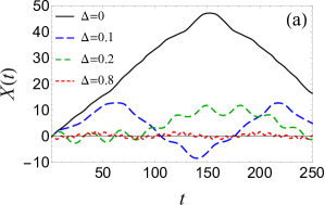
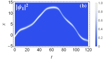
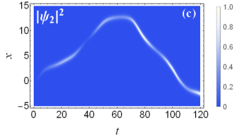
Figure 2: (a) Position of the soliton center of mass as a function of time for different $\Delta$ (marked in the plot), $g=\widetilde{g}=-5,$ and $\alpha=0.4$. Panel (a) shows that for $\Delta=0$ the soliton travels a long distance, whereas switching on the Zeeman field eventually traps it. (b, c) Density plots of the two spinor components in the $(t,x)-$plane for $\Delta=0.1$.

Figure 2 describes the dynamics of the soliton for $\alpha=0.4$ at different values of $\Delta$. The plot shows that, whereas for $\Delta=0$ the soliton moves a long distance through the disordered potential until it is reflected by a large fluctuation of $U(x)$, the presence of a Zeeman field inhibits the propagation, and eventually traps it, for sufficiently large values of $\Delta$ ($=0.8$ in this plot).

In order to better understand this effect of the Zeeman field, we consider Eq. (9) for the velocity, along with the evolution of the spin components. To describe the spin evolution we assume the adiabatic approximation for the soliton evolution (conserving the shape of equal densities of both spin states): ${\bm{\psi}}_{\rm ad}({\mathbf{x}})=\psi_{0}(x-X(t))\exp(ik(t)x)\chi(t),$ where $\chi(t)\equiv\left[\cos(\theta(t)/2)e^{i\phi(t)},\sin(\theta(t)/2)\right]^{\rm T}$ describes corresponding evolution of the spin state. Here “fast” degree of freedom corresponds to the shape of $\psi_{0}(x-X(t))$, while “slow”, lower energy degrees of freedom are described by $k(t)$ and $\chi(t)-$dependencies. In order to define the adiabatic evolution of the spinor $\chi(t)$ we perform spatial “averaging” by multiplying (1) by $\psi_{0}(x-X(t))$ and integrating over $x.$ This gives us an effective Hamiltonian $H_{s}(t)=(\bm{\Omega}(t){\bm{\sigma}})/2$ for the spin motion in a synthetic random Zeeman field as ${\bm{\Omega}}=\left(\Delta,0,2\alpha{k(t)}\right)$, corresponds to the rotation with the rate $\Omega=(4\alpha^{2}k^{2}(t)+\Delta^{2})^{1/2}$ around the randomly time-dependent axis ${\mathbf{n}}={\bm{\Omega}}/\Omega$.

The validity of the adiabatic approximation is corroborated by the fact that the spin state is always close to a pure one (Fig. 3(a)), and the spin is close to the Bloch sphere. In addition, our numerical results show that the shape of the soliton (not shown in the Figures) remains practically unchanged up to $t=300.$ As a result, the velocity (9) self-consistently depends on the evolution of the random effective “magnetic” field. For a large $\Delta\gg\alpha|k(t)|$, the spin is controlled by the Zeeman coupling with $\sigma_{z}(t)\approx\cos{(\Delta t)}$ and, according to Eq. (9), the velocity behaves as $v(t)\approx\alpha\cos(\Delta t).$ For $\Delta\sim{\alpha|k(t)|}$, the behavior of observables becomes much more complicated.

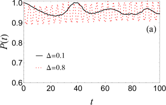
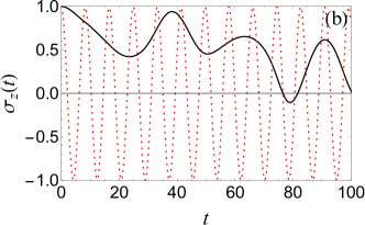
Figure 3: (a) Rescaled purity of the spin state for different $\Delta$ (marked in the plot). The spin is always close to the Bloch sphere, $P^{1/2}(t)\approx 1$. (b) Evolution of the $z$-component of the spin which enters the soliton velocity, see Eq. (9). In both plots $\alpha=0.4$ and $g=\widetilde{g}=-5$.

Since we consider a narrow soliton with the self-interaction energy conserved under the total spin rotations, we can introduce a conserved “low-energy” quantity $\epsilon_{0}$ obtained as the average (1) of the linear part of the Hamiltonian for the adiabatic soliton ${\bm{\psi}}_{\rm ad}({\bf x})$, i.e. ${\epsilon_{0}=}k^{2}(t)/2+\alpha{\sigma}_{z}(t)k(t)+\Delta\sigma_{x}(t)/2+U(X(t)).$ Taking into account that ${\sigma_{z}(t)}=\cos\theta(t),$ $\sigma_{x}(t)=\sin\theta(t)\cos\phi(t),$ the conservation of $\epsilon_{0}$ (verified in the adiabatic approximation) can be presented as

$$v^{2}(t)-{\alpha^{2}}\sigma_{z}^{2}(t)+\Delta\sigma_{x}(t)=2\left[U({X(0)})-U(X(t))\right],$$ (10)

with the velocity $v(t)$ given by Eq. (9). The value $U_{\rm inv}$ of the potential that is sufficient to invert the soliton dynamics, that is $v(t)=0$ at the point where $U(X(t))=U_{\rm inv}$, is obtained by minimization of the sum of the spin-related terms in Eq. (10). Since this minimum is achieved at $\cos\phi=-1$ and $\sin\theta=\min(\Delta/2\alpha^{2},1)$ we obtain $U_{\rm inv}=U(X(0))+\left(\alpha^{2}+\Delta^{2}/4\alpha^{2}\right)/2$ for $\Delta<2\alpha^{2}$, and $U_{\rm inv}=U(X(0))+\Delta/2$ for $\Delta\geq\,2\alpha^{2}.$ Nevertheless, these conditions are not necessary, and the soliton can be stopped already at $U(X(t))<U_{\rm inv}$. At $\Delta=0$ we obtain $U_{\rm inv}=\alpha^{2}/2+U(X(0)),$ corresponding to Fig. 2(a), where $U_{\rm inv}-U(X(0))=0.083$ for $\alpha^{2}/2=0.08.$

Figure 4: Phase trajectory for the values of SOC and Zeeman field marked in the plot for $t<190$. The filled circle describes $\left(X(0),v(0)\right)-$point. The oscillation frequency for $\alpha=0.1$ is $\omega_{\mathrm{s}}=0.094,$ in a good agreement with $\sim{\bar{n}}^{1/4}U_{0}^{1/2}$ estimate. All plots correspond to $g=\widetilde{g}=-5$.

Before discussing other effects, we consider the possibility of experimental realization of the presented system. We remind that the physical units of length and time here are $\xi$ and $t_{\xi}\equiv M\xi^{2}/\hbar$, respectively. The resulting coupling constant $g$ is approximately $2a/\xi\times(\xi/\xi_{\perp})^{2}{\cal N},$ where $\xi_{\perp}$ is the transversal confinement length, $a$ is the interatomic scattering length (e.g., Mardonov2015a ), and ${\cal N}$ is the total number of atoms in the condensate. A typical value of $\xi=3$ $\mu{\rm m}$, with $M$ being the mass of ${}^{7}{\rm Li}$ atom Kevrekidis , corresponds to $t_{\xi}\approx 1$ ms and the unit of velocity $\xi/t_{\xi}\approx 0.3$ cm/s, meaning that our results imply a relatively weak synthetic spin-orbit coupling. The relevant time scale of the studied dynamical phenomena, being of the order of $100$ $t_{\xi}$, is, therefore, within the experimental lifetime of an attractive condensate (see e.g. Trenkwalder2016 ). For typical values of $a$ of the order of $-5\times 10^{-8}$ cm Moerdijk1994 ; Pollack2009 and for a strong confinement $(\xi/\xi_{\perp})^{2}\sim 10,$ we obtain that the required $g=-5$ can be achieved at ${\cal N}\sim 1.5\times 10^{3}$ particles in the condensate. Under these conditions the mean field approach is still well applicable since ${\cal N}\times(|a|^{3}/\xi\xi_{\perp}^{2})\sim|g|\times(a/\xi)^{2}\ll 1.$

III.2 Delocalization induced by spin resonance

Here we will show that in a certain regime, depending on the oscillation frequency, the Zeeman coupling and the SOC, the soliton motion can be characterized by a resonance caused by spin rotation in the Zeeman field. Since this resonance occurs in a nonlinear system, it cannot greatly increase the oscillation amplitude, but it is sufficient to delocalize a soliton in the case of interest. Although in a disordered potential the spin resonance is hardly exactly predictable, it is possible to analyze its effects semiquantitatively. The oscillation frequency $\omega_{\rm s}=2\pi/T$ with the period

$$T=2\int_{a}^{b}\frac{dx}{v(x)},\quad v(x)\equiv\sqrt{2(U(0)-U(x))+\alpha^{2}},$$ (11)

where at the turning points $v(a)=v(b)=0.$ Introducing the critical value $\alpha_{\rm c}^{2}=2[U(x_{r})-U(X(0))],$ we obtain $\omega_{\rm s}\sim\omega_{0}/\ln\left[\alpha_{\rm c}\left(\alpha_{\rm c}-\alpha\right)^{-1}\right],$ where $\omega_{0}\sim{\bar{n}}^{1/4}U_{0}^{1/2}$ is the oscillation frequency near the minimum. Here $x_{r}$ is the position of a strong peak preventing the escape of the soliton (e.g., in Fig. 1, $x_{r}\approx 2.7$). The resonance between the spin and the orbital motion is expected at $\omega_{\rm s}\sim\Delta.$

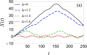
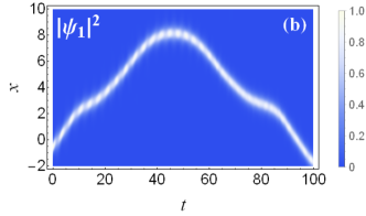
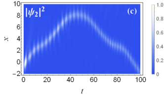
Figure 5: (a) The center of mass position as a function of time for different $\Delta$ and $\widetilde{g}=0,$ $g=-5$. (b), (c) Density plots of the spinor components at $\Delta=1.4$ in the $(t,x)-$ plane. We note two major differences between this figure and Fig. 2 arising due to different symmetries of the self-interaction. First, here one needs an order of magnitude larger Zeeman $\Delta$ to considerably modify the $X(t)-$ dependence. Second, the density distributions of $\left|\psi_{1,2}(x,t)\right|^{2}$ are broader here with the pattern of $\left|\psi_{2}(x,t)\right|^{2}$ demonstrating a clear stripe-like structure.

Figure 4, where we show the velocity as a function of the center of mass position, demonstrates that the interplay between the SOC and the Zeeman field can indeed delocalize the soliton. For example, for $\alpha=0.2$, the delocalization takes place in the range $0.05<\Delta<0.28$. Notice that the escape time, velocity, and the direction are random.

III.3 Vanishing cross-spin coupling, $\widetilde{g}=0$

Now we consider the major differences brought about by the coupling, when only the diagonal self-interaction $g$ is present. For a direct comparison, we begin with the same initial condition as at $\widetilde{g}=g$, that is ${\bm{\psi}}_{\rm in}(x)$. For this realization of nonlinearity, a spin rotation, making $\sigma_{z}(t)$ considerably different from 1, requires a larger $\Delta$ to provide the energy for population transfer between the spinor components $\psi_{1}({\mathbf{x}})$ and $\psi_{2}({\mathbf{x}})$. In order to estimate this Zeeman field and to understand the interplay between the spin rotation and self-interaction, we assume for the moment $U_{0}=\alpha=0$, and consider a “rigid rotation” of the wave function around the $x-$axis, namely: ${\bm{\psi}}(\mathbf{x})=\psi_{0}(x)\left[\cos(\Delta t/2),i\sin(\Delta t/2)\right]^{\rm T}$. For this state, the self-interaction energy corresponding to the $H^{\rm int}$ term in Eq. (1) becomes

$$E_{\rm int}(t)-E_{\rm int}(0)=-E_{\rm int}(0)\sin^{2}\left({\Delta t}\right)/2,$$ (12)

with the maximum $\max\left(E_{\rm int}(t)-E_{\rm int}(0)\right)$ value $|E_{\rm int}(0)|/2={g^{2}}/12$ achieved at $t=\pi/2\Delta.$ On the other hand, the Zeeman energy is $\Delta\sigma_{x}(t)/2.$ It follows from the comparison of these energies that the spin reorientation by the Zeeman coupling can provide sufficient energy for the increase in the self-interaction if $\Delta\gtrsim\Delta_{c}\sim 0.1{g}^{2}$. Consequently, $\Delta_{c}$ being of the order of one at $|g|=5$, considerably exceeds the frequencies $2\pi/T\sim\bar{n}^{1/4}U_{0}^{1/2}$ in Eq. (11). As a result, the Zeeman field causes only the soliton localization, as shown in Fig. 5(a).

The initial rotation populates the spin down component $\psi_{2}(\mathbf{x})$, which is initially vanishing, and therefore not self-interacting. As a result of small population at $t\ll\,1/\Delta$, the relatively weak self interaction cannot prevent the spread of this component, and its broadening begins. At the same time, the decreasing (although never vanishing) population of the upper component becomes insufficient to keep the initial width, and it is broadening as well. The oscillating broadening of $\left|\psi_{2}(\mathbf{x})\right|^{2}$ driven by the Zeeman field is seen as the periodic stripe-like structure in Fig. 5(c).

IV Discussion and conclusions

We have studied the dynamics of the self-attractive quasi one-dimensional Bose-Einstein condensate, forming a bright soliton, in a random potential in the presence of the spin-orbit- and Zeeman couplings. We have found that for given spin-orbit coupling, the soliton motion strongly depends on the Zeeman splitting and on the self-interaction of the condensate. In particular, the Zeeman interaction can lead to localization or delocalization of the soliton due to the spin-dependent anomalous velocity proportional to the spin-orbit coupling. A sufficiently strong Zeeman field can cause localization of the soliton near the random potential minima. If the Zeeman frequency is close to the typical frequency of the soliton oscillations in the random potential, this resonance can cause its delocalization. In the absence of cross-spin interaction, where the Manakov’s symmetry is lifted, the effect of delocalization due to the Zeeman-induced spin rotation is suppressed since a stronger Zeeman field is required here to produce the spin evolution sufficient to modify the center-of-mass motion.

V Acknowledgments

We acknowledge support by the Spanish Ministry of Economy, Industry and Competitiveness (MINECO) and the European Regional Development Fund FEDER through Grant No. FIS2015-67161-P (MINECO/FEDER, UE), and the Basque Government through Grant No. IT986-16. S. M. was partially supported by the Swiss National Foundation SCOPES project IZ74Z0_160527. We are grateful to Y.V. Kartashov for valuable comments.

References

- (1) Y.-J. Lin, R. L. Compton, K. Jiménez-Garcia, J. V. Porto, and I. B. Spielman, Nature 462, 628 (2009).
- (2) Y.-J. Lin, K. Jiménez-García, and I. B. Spielman, Nature 471, 83 (2011).
- (3) H. Zhai, Int. J. Mod. Phys. B 26, 1230001 (2012).
- (4) V. Galitski and I. B. Spielman, Nature 494, 49 (2013).
- (5) H. Zhai, Rep. Prog. Phys. 78, 026001 (2015).
- (6) V. Achilleos, D. J. Frantzeskakis, P. G. Kevrekidis, and D. E. Pelinovsky, Phys. Rev. Lett. 110, 264101 (2013); Y. Xu, Y. Zhang, and B. Wu, Phys. Rev. A 87, 013614 (2013).
- (7) Y.V . Kartashov, V. V. Konotop, and F. K. Abdullaev, Phys. Rev. Lett. 111, 060402 (2013).
- (8) Y. V. Kartashov, V. V. Konotop, and D. A. Zezyulin, Phys. Rev. A, 90, 063621 (2014)
- (9) L. Wen, Q. Sun, Y. Chen, D.-S. Wang, J. Hu, H. Chen, W.-M. Liu, G. Juzeliunas, B. A. Malomed, and A.-C. Ji, Phys. Rev. A 94, 061602(R) (2016).
- (10) E. Chiquillo, Phys. Rev. A 97, 013614 (2018); E. Chiquillo, J. Phys. A: Math. Theor. 48, 475001 (2015).
- (11) B. Ramachandhran, B. Opanchuk, X.-J. Liu, H. Pu, P. D. Drummond, and H. Hu, Phys. Rev. A 85, 023606 (2012).
- (12) T. Kawakami, T. Mizushima, and K. Machida, Phys. Rev. A 84, 011607 (2011).
- (13) H. Sakaguchi and B. Li, Phys. Rev. A 87, 015602 (2013).
- (14) V. E. Lobanov, Y. V. Kartashov, and V. V. Konotop, Phys. Rev. Lett. 112, 180403 (2014).
- (15) X. Y. Huang, F. X. Sun, W. Zhang, Q. Y. He, and C. P. Sun, Phys. Rev. A 95, 013605 (2017).
- (16) A. C. White, Y. Zhang, and T. Busch, Phys. Rev. A 95, 041604(R) (2017).
- (17) H. Sakaguchi, B. Li, and B. A. Malomed, Phys. Rev. E 89, 032920 (2014).
- (18) Y.-C. Zhang, Z.-W. Zhou, B. A. Malomed, and H. Pu, Phys. Rev. Lett. 115, 253902 (2015).
- (19) H. Sakaguchi, E. Ya. Sherman, and B. A. Malomed, Phys. Rev. E 94, 032202 (2016).
- (20) I. Vasić and A. Bala Phys. Rev. A 94, 033627 (2016).
- (21) H. Sakaguchi, B. Li, E. Ya. Sherman, and B. A. Malomed, Romanian Reports in Physics 70, 502 (2018).
- (22) C.-L. Qu, L. P. Pitaevskii, and S. Stringari, New J. Phys. 19, 085006 (2017).
- (23) Y. V. Kartashov, V.V. Konotop, and L. Torner, Phys. Rev. A, 96, 033619 (2017).
- (24) J.-P. Dias, M. Figueira, V.V. Konotop, and D. A. Zezyulin, Stud. Appl. Math. 133, 422 (2015).
- (25) Z.-F. Yu, A.-X. Zhang, R.-A. Tang, H.-P. Xu, J.-M. Gao, and J.-K. Xue, Phys. Rev. A 95, 033607 (2017).
- (26) Z.-F. Yu and J.-K. Xue, Sci. Rep. 7 15635 (2017).
- (27) T. Pertsch, U. Peschel, J. Kobelke, K. Schuster, H. Bartelt, S. Nolte, A. Tünnermann, and F. Lederer, Phys. Rev. Lett. 93, 053901 (2004).
- (28) Y. V. Kartashov and V. A. Vysloukh, Phys. Rev. E 72, 026606 (2005).
- (29) Y. V. Kartashov, V. A. Vysloukh, and L. Torner, Phys. Rev. A 77, 051802 (2008).
- (30) Y. V. Kartashov, V. A. Vysloukh, and L. Torner, Progress in Optics 52, 63 (2009).
- (31) Y. Kartashov, V. Vysloukh, and L. Torner, Opt. Lett. 36, 466 (2011).
- (32) U. Naether, M. Heinrich, Y. Lahini, S. Nolte, R. Vicencio, M. Molina, and A. Szameit, Opt. Lett. 38, 1518 (2013).
- (33) M. Larcher, F. Dalfovo, and M. Modugno, Phys. Rev. A 80, 053606 (2009).
- (34) S. Flach, D. O. Krimer, and Ch. Skokos, Phys. Rev. Lett. 102 024101 (2009).
- (35) I. L. Aleiner, B. L. Altshuler, and G. V. Shlyapnikov, Nat. Phys. 6, 900 (2010).
- (36) C. Fort, L. Fallani, V. Guarrera, J. E. Lye, M. Modugno, D. S. Wiersma, and M. Inguscio, Phys. Rev. Lett. 95, 170410 (2005).
- (37) M. Modugno, Phys. Rev. A 73, 013606 (2006).
- (38) Note that even without self-attraction, the spin-orbit coupled BEC in a random potential demonstrates a nontrivial spin relaxation: Sh. Mardonov, M. Modugno, and E. Ya. Sherman, Phys. Rev. Lett. 115, 180402 (2015).
- (39) M. Modugno, G. Pagnini, and M. A. Valle-Basagoiti, Phys. Rev. A 97, 043604 (2018) and references therein.
- (40) A justification of the use of the Gross-Pitaevskii theory in the presence of disorder can be found in: M. Larcher, T. V. Laptyeva, J. D. Bodyfelt, F. Dalfovo, M. Modugno, and S. Flach, New J. Phys. 14 103036 (2012).
- (41) S. V. Manakov, Sov. Phys. JETP 38, 248 (1974).
- (42) I. V. Tokatly and E. Ya. Sherman, Phys. Rev. A 87 041602 (2013).
- (43) E. N. Adams and E. I. Blount, J. Phys. Chem. Solids 10, 286 (1959).
- (44) The effect of the anomalous velocity in two-dimensional electron systems has been observed experimentally in I. Stepanov, M. Ersfeld, A. V. Poshakinskiy, M. Lepsa, E. L. Ivchenko, S. A. Tarasenko, and B. Beschoten, arXiv:1612.06190.
- (45) J. Armaitis, J. Ruseckas, H. T. C. Stoof, and R. A. Duine, Phys. Rev. A 96, 053625 (2017).
- (46) V. M. Pérez-García, H. Michinel, J. I. Cirac, M. Lewenstein, and P. Zoller, Phys. Rev. A 56, 1424 (1997).
- (47) S. Mardonov, M. Modugno, and E. Ya. Sherman, J. Phys. B: At. Mol. Opt. Phys. 48 115302 (2015).
- (48) A. Trenkwalder, G. Spagnolli, G. Semeghini, S. Coop, M. Landini, P. Castilho, L. Pezze, G. Modugno, M. Inguscio, A. Smerzi, and M. Fattori, Nat. Phys. 12, 826 (2016).
- (49) A. J. Moerdijk, W. C. Stwalley, R. G. Hulet, and B. J. Verhaar, Phys. Rev. Lett. 72, 40 (1994).
- (50) S. E. Pollack, D. Dries, M. Junker, Y. P. Chen, T. A. Corcovilos, and R. G. Hulet, Phys. Rev. Lett. 102, 090402 (2009).