Regularized Zero-Forcing Precoding Aided Adaptive Coding and Modulation for Large-Scale Antenna Array Based Air-to-Air Communications

Abstract

We propose a regularized zero-forcing transmit precoding (RZF-TPC) aided and distance-based adaptive coding and modulation (ACM) scheme to support aeronautical communication applications, by exploiting the high spectral efficiency of large-scale antenna arrays and link adaption. Our RZF-TPC aided and distance-based ACM scheme switches its mode according to the distance between the communicating aircraft. We derive the closed-form asymptotic signal-to-interference-plus-noise ratio (SINR) expression of the RZF-TPC for the aeronautical channel, which is Rician, relying on a non-centered channel matrix that is dominated by the deterministic line-of-sight component. The effects of both realistic channel estimation errors and of the co-channel interference are considered in the derivation of this approximate closed-form SINR formula. Furthermore, we derive the analytical expression of the optimal regularization parameter that minimizes the mean square detection error. The achievable throughput expression based on our asymptotic approximate SINR formula is then utilized as the design metric for the proposed RZF-TPC aided and distance-based ACM scheme. Monte-Carlo simulation results are presented for validating our theoretical analysis as well as for investigating the impact of the key system parameters. The simulation results closely match the theoretical results. In the specific example that two communicating aircraft fly at a typical cruising speed of 920 km/h, heading in opposite direction over the distance up to 740 km taking a period of about 24 minutes, the RZF-TPC aided and distance-based ACM is capable of transmitting a total of 77 Gigabyte of data with the aid of 64 transmit antennas and 4 receive antennas, which is significantly higher than that of our previous eigen-beamforming transmit precoding aided and distance-based ACM benchmark.

I Introduction

The vision of the ‘smart sky’ [1] in support of air traffic control and the ‘Internet above the clouds’ [2] for in-flight entertainment has motivated researchers to develop new solutions for aeronautical communications. The aeronautical ad hoc network (AANET) [3] exchanges information using multi-hop air-to-air radio communication links, which is capable of substantially extending the coverage range over the oceanic and remote airspace, without any additional infrastructure and without relying on satellites. However, the existing air-to-air communication solutions can only provide limited data rates. Explicitly, the planed L-band digital aeronautical communications system (L-DACS) [4, 5] only provides upto 1.37 Mbps air-to-ground communication rate, and the aeronautical mobile airport communication system [6] only offers 9.2 Mbps air-to-ground communication rate in the vicinity of the airport. Finally, the L-DACS air-to-air mode [7] is only capable of providing 273 kbps net user rate for direct air-to-air communication, which cannot meet the high-rate demands of the emerging aeronautical applications.

The existing aeronautical communication systems mainly operate in the very high frequency band spanning from 118 MHz to 137 MHz [8], and there are no substantial idle frequency slots for developing broadband commercial aeronautical communications. Moreover, the ultra high frequency band has almost been fully occupied by television broadcasting, cell phones and satellite communications [1, 9]. However, there are many unlicensed-frequencies in the super high frequency (SHF) band spanning from 3 GHz to 30 GHz, which may be explored for the sake of developing broadband commercial aeronautical communications. Explicitly, the wavelength spans from 1 cm to 10 cm for the SHF band, which results in 0.5 cm $\sim$ 5 cm antenna spacing by utilizing the half-wavelength criterion for designing the antenna array. This antenna spacing is capable of accommodating a large-scale antenna array on commercial aircraft, which offers dramatic throughput and energy efficiency benefits [10]. To provide a high throughput and a high spectral efficiency (SE) for commercial air-to-air applications, we propose a large-scale antenna array aided adaptive coding and modulation (ACM) based solution in the SHF band.

As an efficient link adaptation technique, ACM [11, 12] adaptively matches the modulation and coding modes to the conditions of the propagation link, which is capable of enhancing the link reliability and maximizing the throughput. The traditional ACM relies on the instantaneous signal-to-noise ratio (SNR) or signal-to-interference-plus-noise ratio (SINR) to switch the ACM modes, which requires the acquisition of the instantaneous channel state information (CSI). Naturally, channel estimation errors are unavoidable in practice, especially at aircraft velocities [13]. Furthermore, the CSI-feedback based ACM solution may potentially introduce feedback errors and delays [14]. Intensive investigations have been invested in robust ACM, relying on partial CSI [13] and imperfect CSI [15], or exploiting non-coherent detection for dispensing with channel estimation all together [16]. However, all these ACM solutions are designed for terrestrial wireless communications and they have to frequently calculate the SINR and to promptly change the ACM modes, which imposes heavy mode-signaling overhead. Therefore, for air-to-air communications, these ACM designs may become impractical.

Unlike terrestrial channels, which typically exhibit Rayleigh characteristics, aeronautical communication channels exhibit strong line-of-sight (LOS) propagation characteristics [17, 18], and at cruising altitudes, the LOS component dominates the reflected components. Furthermore, the passenger planes typically fly across large-scale geographical distances, and the received signal strength is primarily determined by the pathloss, which is a function of communication distance. In [19], we proposed an eigen-beamforming transmit precoding (EB-TPC) aided and distance-based ACM solution for air-to-air aeronautical communication by exploiting the aeronautical channel characteristics. EB-TPC has the advantage of low-complexity operation by simply conjugating the channel matrix, and it also enables us to derive the closed-form expression of the attainable throughput, which facilitates the design of the distance-based ACM [19]. However, its achievable throughput is far from optimal, since EB-TPC does not actively suppress the inter-antenna interference. Zero-forcing transmit precoding (ZF-TPC) [20] by contrast is capable of mitigating the inter-antenna interference, but it is challenging to provide a closed-form expression for the achievable throughput, particularly for large-scale antenna array based systems. Tataria et al. [21] investigated the distribution of the instantaneous per-terminal SNR for the ZF-TPC aided multi-user system and approximated it as a gamma distribution. Additionally, ZF-TPC also surfers from rate degradation in ill-conditioned channels. By introducing regularization, the regularized ZF-TPC (RZF-TPC) [22] is capable of mitigating the ill-conditioning problem by beneficially balancing the interference cancellation and the noise enhancement [23]. Furthermore, owing to the regularization, it becomes possible to analyze the achievable throughput for the Rayleigh fading channel. Hoydis et al. [24] used the RZF-TPC as the benchmark to study how many extra antennas are needed for the EB-TPC in the context of Rayleigh fading channels.

However, the Rician fading channel experienced in aeronautical communications, which has a non-centered channel matrix due to the presence of the deterministic LOS component, is different from the centered Rayleigh fading channel. This imposes a challenge on deriving a closed-form formula of the achievable throughput, which is a fundamental metric of designing ACM solutions. Few researches have tackled this challenge. Nonetheless, recently three conference papers [25, 26, 27] have investigated the asymptotic sum-rate of the RZF-TPC in Rician channels. Explicitly, Tataria et al. [25] investigated the ergodic sum-rate of the RZF-TPC aided single-cell system under the idealistic condition of uncorrelated Rician channel and the idealistic assumption of perfect channel knowledge. Falconet et al. [26] provided an asymptotic sum-rate expression for RZF-TPC in a single-cell scenario by assuming identical fading-correlation for all the users. Sanguinetti et al. [27] extended this work from the single-cell to the coordinated multi-cell scenario under the same assumption. But crucially, the authors of [27] did not consider the pilot contamination imposed by adjacent cells during the uplink channel estimation [28, 29]. Moreover, the study [27] assumed Rician fading only within the serving cell, while the interfering signals arriving from adjacent cells were still assumed to suffer from Rayleigh fading. This assumption has limited validity in aeronautical communications. Most critically, the asymptotic sum-rates provided in [26] and [27] were based on the assumption that both the number of antennas and the number of served users tend to infinity. The essence of the ‘massive’ antenna array systems is that of serving a small number of users on the same resource block using linear signal processing by employing a large number of antenna elements. Assuming that the number of users on a resource block tends to infinity has no physical foundation at all.

Against this background, this paper designs an RZF-TPC scheme for large-scale antenna array assisted and distance-based ACM aided aeronautical communications, which offers an appealing solution for supporting the emerging Internet above the clouds. Our main contributions are:

1. We derive the closed-form expression of the achievable throughput for the RZF-TPC in the challenging new context of aeronautical communications. Our previous contribution work relying on EB-TPC [19] invoked relatively simple analysis, since it did not involve the non-centered channel matrix inverse. By contrast, the derivation of the closed-form throughput of our new RZF-TPC has to tackle the associated non-centered matrix inverse problem. Moreover, in contrast to the EB-TPC, the regularization parameter of the RZF-TPC has to be optimized for maximizing the throughput. In this paper, we derive the closed-form asymptotic approximation of the SINR for the RZF-TPC in the presence of both realistic channel estimation errors and co-channel interference imposed by the aircraft operating in the same frequency band. We also provide the associated detailed proof. Moreover, we explicitly derive the optimal analytical regularization parameter that minimizes the mean square detection error. Given this asymptotic approximation of the SINR, the fundamental metric of the achievable throughput as the function of the communication distance is provided for designing the distance-based ACM.

2. We develop the new RZF-TPC aided and distance-based ACM design for the application to the large antenna array assisted aeronautical communication in the presence of imperfect CSI and co-channel interference, first considered in [19]. Like our previous EB-TPC aided and distance-based ACM scheme [19], the RZF-TPC aided and distance-based ACM scheme switches its ACM mode based on the distance between the communicating aircraft pair. However, the RZF-TPC is much more powerful, and the proposed design offers significantly higher SE over the previous EB-TPC aided and distance-based ACM design. Specifically, the new design achieves up to 3.0 bps/Hz and 3.5 bps/Hz SE gains with the aid of 32 transmit antennas/4 receive antennas and 64 transmit antennas/4 receive antennas, respectively, over our previous design.

II System Model

We consider an air-to-air communication scenario at cruising altitude. Our proposed time division duplex (TDD) based aeronautical communication system is illustrated Fig. 1. In the communication zone considered, aircraft $a^{*}$ transmits its data to aircraft $b^{*}$, while aircraft $a$, $a=1,2,\cdots,A$ are the interfering aircraft using the same frequency as aircraft $a^{*}$ and $b^{*}$. The aeronautical communication system operates in the SHF band and we assume that the carrier frequency is 5 GHz, which results in a wave-length of 6 cm. Thus, it is practical to accommodate a large-scale high-gain antenna array on the aircraft for achieving high SE. We assume furthermore that all the aircraft are equipped with the same large-scale antenna array. Specifically, each aircraft has $N_{\rm total}$ antennas, which transmit and receive signals on the same frequency. Explicitly, each aircraft utilizes $N_{t}$ ($<N_{\rm total}$) antennas, denoted as data-transmitting antennas (DTAs), for transmitting data and utilizes $N_{r}$ antennas, denoted as data-receiving antennas (DRAs), for receiving data. In line with the maximum attainable spatial degrees of freedom, generally, we have $N_{r}<N_{t}$. Furthermore, the system adopts orthogonal frequency-division multiplexing (OFDM) for improving the SE and the TDD protocol for reducing the latency imposed by channel information feedback. Each aircraft has a distance measuring equipment (DME), e.g., radar, which is capable of measuring the distance to nearby aircraft. Alternatively, the GPS system may be utilized to provide the distance information required.

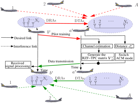
Figure 1: The proposed aeronautical communication system employing the RZF-TPC aided and distance-based ACM scheme, where aircraft $a^{*}$ is transmitting data to aircraft $b^{*}$ in the presence of co-channel interference.

II-A Channel State Information Acquisition

In order to transmit data from $a^{*}$ to $b^{*}$, aircraft $a^{*}$ needs the CSI linking $a^{*}$ to aircraft $b^{*}$. Aircraft $a^{*}$ estimates the reverse channel based on the pilots sent by $b^{*}$, and then exploits the channel’s reciprocity of TDD protocol to acquire the required CSI. Explicitly, this pilot training phase is shown at the top of Fig. 1, where $a^{*}$ estimates the channel between the $N_{r}$ DRAs of $b^{*}$ and its $N_{t}$ DTAs based on the pilots sent by $b^{*}$ in the presence of the interference imposed by the aircraft $a$, $a=1,2,\cdots,A$. We consider the worst-case scenario, where the interfering aircraft $a$ also transmits the same pilot symbols as $b^{*}$, which results in the most serious co-channel interference. Since the length of the cyclic prefix (CP) $N_{\rm cp}$ is longer than the channel length $P$, inter-symbol interference is completely eliminated, and the receiver can process the signals on a subcarrier-by-subcarrier basis. Thus, the frequency-domain (FD) signal vector of $a^{*}$, $\widetilde{\bm{Y}}_{a^{*}}=\big{[}\widetilde{Y}^{a^{*}}_{1}~{}\widetilde{Y}^{a^{*}}_{2}\cdots\widetilde{Y}^{a^{*}}_{N_{t}}\big{]}^{\rm T}\in\mathbb{C}^{N_{t}}$, received during the pilot training can be written as

$$\widetilde{\bm{Y}}_{a^{*}}=\sqrt{P_{r,a^{*}}^{b^{*}}}\bm{H}_{a^{*}}^{b^{*}}\widetilde{\bm{X}}^{b^{*}}+\sum\limits_{a=1}^{A}\sqrt{P_{r,a^{*}}^{a}}\bm{H}_{a^{*}}^{a}\widetilde{\bm{X}}^{a}+\widetilde{\bm{W}}_{a^{*}},$$ (1)

where $\widetilde{\bm{X}}^{b^{*}}=\big{[}\widetilde{X}^{b^{*}}_{1}~{}\widetilde{X}^{b^{*}}_{2}\cdots\widetilde{X}^{b^{*}}_{N_{r}}\big{]}^{\rm T}\in\mathbb{C}^{N_{r}}$ is the pilot symbol vector transmitted by $b^{*}$, which obeys the complex Gaussian distribution with the mean vector of the $N_{r}$-dimensional zero vector $\bm{0}_{N_{r}}$ and the covariance matrix of the $N_{r}\times N_{r}$ identity matrix $\bm{I}_{N_{r}}$, denoted by $\widetilde{\bm{X}}^{b^{*}}\sim\mathcal{CN}\left(\bm{0}_{N_{r}},\bm{I}_{N_{r}}\right)$, and $\bm{H}_{a^{*}}^{a^{\prime}}\in\mathbb{C}^{N_{t}\times N_{r}}$ denotes the FD channel transfer function coefficient matrix linking the $N_{r}$ DRAs of $a^{\prime}$ to the $N_{t}$ DTAs of $a^{*}$, for $a^{\prime}=b^{*},a$, while $\widetilde{\bm{W}}_{a^{*}}\sim\mathcal{CN}\left(\bm{0}_{N_{t}},\sigma_{w}^{2}\bm{I}_{N_{t}}\right)$ is the FD additive white Gaussian noise (AWGN) vector, and $P_{r,a^{*}}^{b^{*}}$ and $P_{r,a^{*}}^{a}$ represent the received powers at a single DTA of $a^{*}$ for the signals transmitted from $b^{*}$ and $a$, respectively. Moreover, since the worst-case scenario is considered, aircraft $a$ uses the same pilot symbol as $b^{*}$, and we have $\widetilde{\bm{X}}^{a}=\widetilde{\bm{X}}^{b^{*}}$ for $1\leq a\leq A$.

Typically, the aeronautical channel consists of a strong LOS path and a cluster of reflected/delayed paths [17, 30, 31]. Hence, the channel is Rician, and $\bm{H}_{a^{*}}^{b^{*}}\in\mathbb{C}^{N_{t}\times N_{r}}$ is given by

$$\bm{H}_{a^{*}}^{b^{*}}= \nu\bm{H}_{\text{d},a^{*}}^{b^{*}}+\varsigma\bm{H}_{\text{r},a^{*}}^{b^{*}},$$ (2)

where $\bm{H}_{{\rm d},a^{*}}^{b^{*}}\in\mathbb{C}^{N_{t}\times N_{r}}$ and $\bm{H}_{{\rm r},a^{*}}^{b^{*}}\in\mathbb{C}^{N_{t}\times N_{r}}$ are the deterministic and scattered channel components, respectively, while $\nu=\sqrt{\frac{K_{\rm Rice}}{K_{\rm Rice}+1}}$ and $\varsigma=\sqrt{1-\nu}$, in which $K_{\rm Rice}$ is the Rician $K$-factor of the channel. When aircraft are at cruising altitude, the deterministic LOS component dominates, and the scattered component is very weak which may come from the reflections from other distant aircraft or tall mountains. Note that when an aircraft is at cruising altitude, there is no local scatters at all, because a minimum safe distance is enforced among aircraft, and there exists no shadowing effect either. For an aircraft near airport space for landing/takeoff, the scattering component is much stronger than at cruising, but the LOS component still dominates. The scattering component in this case includes reflections from ground, and shadowing effect has to be considered. The scattered component $\bm{H}_{\text{r},a^{*}}^{b^{*}}$ can be expressed as [32]

$$\bm{H}_{\text{r},a^{*}}^{b^{*}}= \bm{R}_{a^{*}}^{\frac{1}{2}}\bm{G}_{a^{*}}^{b^{*}}\big{(}\bm{R}^{b^{*}}\big{)}^{\frac{1}{2}},$$ (3)

where $\bm{R}^{b^{*}}\in\mathbb{C}^{N_{r}\times N_{r}}$ and $\bm{R}_{a^{*}}\in\mathbb{C}^{N_{t}\times N_{t}}$ are the spatial correlation matrices for the $N_{r}$ antennas of $b^{*}$ and the $N_{t}$ antennas of $a^{*}$, respectively, while the elements of $\bm{G}_{a^{*}}^{b^{*}}\in\mathbb{C}^{N_{t}\times N_{r}}$ follow the independently identically distributed distribution $\mathcal{CN}(0,1)$. Thus, $\mathcal{E}\left\{\bm{vec}\left(\bm{H}_{{\rm r},a^{*}}^{b^{*}}\right)\right\}=\bm{0}_{N_{t}N_{r}}$, where $\mathcal{E}\{\cdot\}$ is the expectation operator and $\bm{vec}(\bm{H})$ denotes the column stacking operation applied to $\bm{H}$, while the covariance matrix $\bm{R}_{{\rm r},a^{*}}^{b^{*}}=\mathcal{E}\left\{\bm{vec}\left(\bm{H}_{{\rm r},a^{*}}^{b^{*}}\right)\bm{vec}^{\rm H}\left(\bm{H}_{{\rm r},a^{*}}^{b^{*}}\right)\right\}\in\mathbb{C}^{N_{t}N_{r}\times N_{t}N_{r}}$ is given by $\bm{R}_{{\rm r},a^{*}}^{b^{*}}=\bm{R}^{b^{*}}\otimes\bm{R}_{a^{*}}$, in which $\otimes$ is the Kronecker product. Since all the aircraft are assumed to be equipped with the same antenna array, we will assume that all the $\bm{R}_{a_{t}}$, $\forall a_{t}\in\mathcal{A}=\{1,2,\cdots,A,a^{*},b^{*}\}$, are equal, i.e., we have $\bm{R}_{a_{t}}=\bar{\bm{R}}_{t}$, $\forall a_{t}\in\mathcal{A}$, and all the $\bm{R}^{a_{r}}$ are equal, namely, $\bm{R}^{a_{r}}=\bar{\bm{R}}^{r}$, $\forall a_{r}\in\mathcal{A}$. Hence, all the covariance matrices are equal, and they can be expressed as

$$\bm{R}_{\text{r},a_{t}}^{a_{r}}= \bar{\bm{R}}_{\text{r},t}^{r}=\bar{\bm{R}}^{r}\otimes\bar{\bm{R}}_{t},\,\forall a_{t},a_{r}\in\mathcal{A}\text{ and }a_{t}\neq a_{r}.$$ (4)

Note that in practice, $N_{r}\ll N_{t}$ and, therefore, the DRAs can always be spaced sufficiently apart so that they become uncorrelated. Consequently, we have $\bar{\bm{R}}^{r}=\bm{I}_{N_{r}}$.

According to [34], the received power $P_{r,a^{*}}^{b^{*}}$ at a single DTA antenna of aircraft $a^{*}$ is related to the transmitted signal power $P_{t}^{b^{*}}$ at a single DRA antenna of $b^{*}$ by

$$P_{r,a^{*}}^{b^{*}}=P_{t}^{b^{*}}10^{-0.1L_{{\rm pathloss},a^{*}}^{b^{*}}}.$$ (5)

Since we mainly consider air-to-air transmissions, there exists no shadowing, and the pathloss model can be expressed as [34]

$$L_{\text{path loss},a^{*}}^{b^{*}}\,[\text{dB}]=-154.06+20\log_{10}\left(f\right)+20\log_{10}\left(d\right),$$ (6)

where $f$ [Hz] is the carrier frequency and $d$ [m] is the distance between the communicating aircraft pair. For the received interference signal power $P_{r,a^{*}}^{a}$, we have a similar pathloss model. For air-to-ground communication near airport space, it may need to consider shadowing effect, and the shadow fading standard deviation in dB should be added to the pathloss model [35].

The minimum mean square error (MMSE) estimate $\widehat{\bm{H}}_{a^{*}}^{b^{*}}$ of $\bm{H}_{a^{*}}^{b^{*}}$ is given by [36]

$$\bm{vec}\left(\widehat{\bm{H}}_{a^{*}}^{b^{*}}\right)= \bm{vec}\left(\nu\bm{H}_{\text{d},a^{*}}^{b^{*}}\right)+\varsigma^{2}\bar{\bm{R}}_{\text{r},t}^{r}\left(\frac{\sigma_{w}^{2}}{P_{r,a^{*}}^{b^{*}}}\bm{I}_{N_{r}N_{t}}+\varsigma^{2}\bar{\bm{R}}_{\text{r},t}^{r}+\sum\limits_{a=1}^{A}\frac{P_{r,a^{*}}^{a}}{P_{r,a^{*}}^{b^{*}}}\varsigma^{2}\bar{\bm{R}}_{\text{r},t}^{r}\right)^{-1}$$

$$\times\bigg{(}\bm{vec}\left(\varsigma\bm{H}_{\text{r},a^{*}}^{b^{*}}\right)+\sum\limits_{a=1}^{A}\sqrt{\frac{P_{r,a^{*}}^{a}}{P_{r,a^{*}}^{b^{*}}}}\bm{vec}\left(\varsigma\bm{H}_{\text{r},a^{*}}^{a}\right)+\frac{1}{\sqrt{P_{r,a^{*}}^{b^{*}}}}\bm{vec}\left(\widetilde{\bar{\bm{W}}}_{a^{*}}\Big{(}\widetilde{\bar{\bm{X}}}^{b^{*}}\Big{)}^{\rm H}\right)\bigg{)}\!,$$ (7)

where $\widetilde{\bar{\bm{X}}}^{b^{*}}\in\mathbb{C}^{N_{r}\times N_{r}}$ consists of the $N_{r}$ consecutive pilot symbols with $\widetilde{\bar{\bm{X}}}^{b^{*}}\big{(}\widetilde{\bar{\bm{X}}}^{b^{*}}\big{)}^{\rm H}=\bm{I}_{N_{r}}$, and $\widetilde{\bar{\bm{W}}}_{a^{*}}\in\mathbb{C}^{N_{r}\times N_{r}}$ is the corresponding AWGN matrix over the $N_{r}$ consecutive OFDM symbols. Explicitly, the distribution of the MMSE estimator (II-A) is [36]

$$\bm{vec}\left(\widehat{\bm{H}}_{a^{*}}^{b^{*}}\right)\sim\mathcal{CN}\left(\bm{vec}\left(\nu\bm{H}_{\text{d},a^{*}}^{b^{*}}\right),\bm{\Phi}_{a^{*}}^{b^{*}}\right),$$ (8)

whose covariance matrix $\bm{\Phi}_{a^{*}}^{b^{*}}\in\mathbb{C}^{N_{t}N_{r}\times N_{t}N_{r}}$ is given by

$$\bm{\Phi}_{a^{*}}^{b^{*}}= \varsigma^{2}\bar{\bm{R}}_{\text{r},t}^{r}\left(\frac{\sigma_{w}^{2}}{P_{r,a^{*}}^{b^{*}}}\bm{I}_{N_{r}N_{t}}\!+\!\varsigma^{2}\bar{\bm{R}}_{\text{r},t}^{r}\!+\!\sum\limits_{a=1}^{A}\frac{P_{r,a^{*}}^{a}}{P_{r,a^{*}}^{b^{*}}}\varsigma^{2}\bar{\bm{R}}_{\text{r},t}^{r}\right)^{-1}\varsigma^{2}\bar{\bm{R}}_{\text{r},t}^{r}.$$ (9)

By defining $\bm{\Phi}_{a^{*}}=\mathcal{E}\left\{\widehat{\bm{H}}_{{\rm r},a^{*}}^{b^{*}}\left(\widehat{\bm{H}}_{{\rm r},a^{*}}^{b^{*}}\right)^{\rm H}\right\}\in\mathbb{C}^{N_{t}\times N_{t}}$ and $\bm{\Phi}^{b^{*}}=\mathcal{E}\left\{\left(\widehat{\bm{H}}_{{\rm r},a^{*}}^{b^{*}}\right)^{\rm H}\widehat{\bm{H}}_{{\rm r},a^{*}}^{b^{*}}\right\}\in\mathbb{C}^{N_{r}\times N_{r}}$, where $\widehat{\bm{H}}_{{\rm r},a^{*}}^{b^{*}}$ denotes the estimate of $\bm{H}_{{\rm r},b^{*}}^{a^{*}}$, $\bm{\Phi}_{a^{*}}^{b^{*}}$ can be expressed as

$$\bm{\Phi}_{a^{*}}^{b^{*}}= \bm{\Phi}_{a^{*}}\otimes\bm{\Phi}^{b^{*}}.$$ (10)

According to Lemma 1 of [37], $\bm{\Phi}^{b^{*}}\to\bm{I}_{N_{r}}$ as $N_{t}\to\infty$. Since $N_{t}$ is large, we have $\bm{\Phi}^{b^{*}}\approx\bm{I}_{N_{r}}$. Hence, given $\bm{\Phi}_{a^{*}}^{b^{*}}$, $\bm{\Phi}_{a^{*}}$ is uniquely determined. It is well known that the computational complexity of this optimal MMSE channel estimator is on the order of $\textsf{O}\big{(}N_{r}^{3}N_{t}^{3}\big{)}$.

II-B Data Transmission

During the data transmission, $a^{*}$ transmits the data vector $\bm{X}^{a^{*}}=\big{[}X_{1}^{a^{*}}~{}X_{2}^{a^{*}}\cdots X_{N_{r}}^{a^{*}}\big{]}^{\rm T}\in\mathbb{C}^{N_{r}}$ using its $N_{t}$ DTAs to the $N_{r}$ DRAs of $b^{*}$, in the presence of the co-channel interference imposed by other aircraft, as shown at the bottom of Fig. 1. Owing to the TDD channel reciprocity, the channel $\bm{H}_{b^{*}}^{a^{*}}\in\mathbb{C}^{N_{r}\times N_{t}}$ encountered by transmitting $\bm{X}^{a^{*}}$ is $\bm{H}_{b^{*}}^{a^{*}}=\left(\bm{H}_{a^{*}}^{b^{*}}\right)^{\rm H}$ and its estimate is given by $\widehat{\bm{H}}_{b^{*}}^{a^{*}}=\left(\widehat{\bm{H}}_{a^{*}}^{b^{*}}\right)^{\rm H}$, which is used for designing the transmit precoding (TPC) for mitigating the inter-antenna interference (IAI). We adopt the powerful RZF-TPC whose TPC matrix $\bm{V}_{b^{*}}^{a^{*}}\in\mathbb{C}^{N_{t}\times N_{r}}$ is given by

$$\bm{V}_{b^{*}}^{a^{*}}= \bm{\Upsilon}_{b^{*}}^{a^{*}}(\widehat{\bm{H}}_{b^{*}}^{a^{*}})^{\rm H},$$ (11)

with

$$\bm{\Upsilon}_{b^{*}}^{a^{*}}= \left(\frac{1}{N_{t}}(\widehat{\bm{H}}_{b^{*}}^{a^{*}})^{\rm H}\widehat{\bm{H}}_{b^{*}}^{a^{*}}+\xi_{b^{*}}^{a^{*}}\bm{I}_{N_{t}}\right)^{-1},$$ (12)

where $\xi_{b^{*}}^{a^{*}}>0$ is the regularization parameter. It can be seen that the complexity of calculating the TPC matrix for the RZF-TPC scheme is on the order of $\textsf{O}\big{(}N_{t}^{3}\big{)}$. Given $\bm{V}_{b^{*}}^{a^{*}}$, the received signal vector $\bm{Y}_{b^{*}}\in\mathbb{C}^{N_{r}}$ of aircraft $b^{*}$ can be written as

$$\bm{Y}_{b^{*}}= \sqrt{P_{r,b^{*}}^{a^{*}}}\bm{H}_{b^{*}}^{a^{*}}\bm{V}_{b^{*}}^{a^{*}}\bm{X}^{a^{*}}\!+\!\sum\limits_{a=1}^{A}\sqrt{P_{r,b^{*}}^{a}}\bm{H}_{b^{*}}^{a}\bm{V}_{b^{a}}^{a}\bm{X}^{a}\!+\!\bm{W}_{b^{*}},$$ (13)

where aircraft $a$ uses the RZF-TPC matrix $\bm{V}_{b^{a}}^{a}\in\mathbb{C}^{N_{t}\times N_{r}}$ to transmit the data vector $\bm{X}^{a}=\big{[}X_{1}^{a}~{}X_{2}^{a}\cdots X_{N_{r}}^{a}\big{]}^{\rm T}$ to its desired receiving aircraft $b^{a}$ for $1\leq a\leq A$, $b^{a}\neq b^{*}$ and $b^{a}\neq a$, and hence $\sqrt{P_{r,b^{*}}^{a}}\bm{H}_{b^{*}}^{a}\bm{V}_{b^{a}}^{a}\bm{X}^{a}$ is the interference imposed by $a$, while the AWGN vector $\bm{W}_{b^{*}}=\big{[}W_{1}^{b^{*}}~{}W_{2}^{b^{*}}\cdots W_{N_{r}}^{b^{*}}\big{]}^{\rm T}$ has the distribution $\mathcal{CN}\big{(}\bm{0}_{N_{r}},\sigma_{w}^{2}\bm{I}_{N_{r}}\big{)}$. By using $[\bm{A}]_{[n:~{}]}$ and $[\bm{A}]_{[~{}:m]}$ to denote the $n$-th row and $m$-th column of $\bm{A}$, respectively, the signal received by the $n_{r}^{*}$-th antenna of aircraft $b^{*}$ can be expressed as

$$Y^{b^{*}}_{n_{r}^{*}}= \sqrt{P_{r,b^{*}}^{a^{*}}}\left[\bm{H}_{b^{*}}^{a^{*}}\right]_{[n_{r}^{*}:~{}]}\left[\bm{V}_{b^{*}}^{a^{*}}\right]_{[~{}:n_{r}^{*}]}X_{n_{r}^{*}}^{a^{*}}+\sum\limits_{n_{r}\neq n_{r}^{*}}\sqrt{P_{r,b^{*}}^{a^{*}}}\left[\bm{H}_{b^{*}}^{a^{*}}\right]_{[n_{r}^{*}:~{}]}\left[\bm{V}_{b^{*}}^{a^{*}}\right]_{[~{}:n_{r}]}X_{n_{r}}^{a^{*}}$$

$$+\sum\limits_{a=1}^{A}\sum\limits_{n_{r}=1}^{N_{r}}\sqrt{P_{r,b^{*}}^{a}}\left[\bm{H}_{b^{*}}^{a}\right]_{[n_{r}^{*}:~{}]}\left[\bm{V}_{b^{a}}^{a}\right]_{[~{}:n_{r}]}X_{n_{r}}^{a}+W^{b^{*}}_{n_{r}^{*}}.$$ (14)

where the first term in the right-hand side of (II-B) is the desired signal, the second term represents the IAI imposed by the $n_{r}$ antennas of aircraft $b^{*}$ for $n_{r}\neq n_{r}^{*}$ on the desired signal, and the third term is the interference imposed by aircraft $a$ for $1\leq a\leq A$ on the desired signal.

III Analysis of Achievable Throughput of RZF-TPC

Since $b^{*}$ does not know the estimated CSI, the achievable ergodic rate is adopted. We will also take into account the channel estimation error. From the signal $Y^{b^{*}}_{n_{r}^{*}}$ (II-B) received at the DRA $n_{r}^{*}$ of $b^{*}$, the power of the desired signal $P_{{\rm S}_{b^{*},n_{r}^{*}}^{a^{*}}}$ and the power of the interference pulse noise $P_{{\rm I\&N}_{b^{*},n_{r}^{*}}^{a^{*}}}$ can be obtained respectively as

$$P_{{\rm S}_{b^{*},n_{r}^{*}}^{a^{*}}}= P_{r,b^{*}}^{a^{*}}\left|\mathcal{E}\left\{\left[\bm{H}_{b^{*}}^{a^{*}}\right]_{[n_{r}^{*}:~{}]}\left[\bm{V}_{b^{*}}^{a^{*}}\right]_{[~{}:n_{r}^{*}]}\right\}\right|^{2},$$ (15)

$$P_{{\rm I\&N}_{b^{*},n_{r}^{*}}^{a^{*}}}= P_{r,b^{*}}^{a^{*}}\text{Var}\left\{\left[\bm{H}_{b^{*}}^{a^{*}}\right]_{[n_{r}^{*}:~{}]}\left[\bm{V}_{b^{*}}^{a^{*}}\right]_{[~{}:n_{r}^{*}]}\right\}+P_{r,b^{*}}^{a^{*}}\sum\limits_{n_{r}\neq n_{r}^{*}}\mathcal{E}\left\{\left|\left[\bm{H}_{b^{*}}^{a^{*}}\right]_{[n_{r}^{*}:~{}]}\left[\bm{V}_{b^{*}}^{a^{*}}\right]_{[~{}:n_{r}]}\right|^{2}\right\}$$

$$+\sum\limits_{a=1}^{A}P_{r,b^{*}}^{a}\sum\limits_{n_{r}=1}^{N_{r}}\mathcal{E}\left\{\left|\left[\bm{H}_{b^{*}}^{a}\right]_{[n_{r}^{*}:~{}]}\left[\bm{V}_{b^{a}}^{a}\right]_{[~{}:n_{r}]}\right|^{2}\right\}+\sigma_{w}^{2},$$ (16)

where $\text{Var}\left\{~{}\right\}$ is the variance operator. Thus, the SINR at $n_{r}^{*}$-th DRA of $b^{*}$ is given by

$$\gamma_{b^{*},n_{r}^{*}}^{a^{*}}= \frac{P_{{\rm S}_{b^{*},n_{r}^{*}}^{a^{*}}}}{P_{{\rm I\&N}_{b^{*},n_{r}^{*}}^{a^{*}}}},$$ (17)

and the achievable transmission rate per antenna between the transmitting aircraft $a^{*}$ and the destination aircraft $b^{*}$ can be readily expressed as

$$C_{b^{*}}^{a^{*}}= \frac{1}{N_{r}}\sum\limits_{n_{r}^{*}=1}^{N_{r}}\log_{2}\left(1+\gamma_{b^{*},n_{r}^{*}}^{a^{*}}\right).$$ (18)

III-A Statistics of Channel Estimate

The MMSE channel estimate $\left[\widehat{\bm{H}}_{b^{*}}^{a^{*}}\right]_{[n_{r}:~{}]}$ is related to the true channel $\left[\bm{H}_{b^{*}}^{a^{*}}\right]_{[n_{r}:~{}]}$ by

$$\left[\bm{H}_{b^{*}}^{a^{*}}\right]_{[n_{r}:~{}]}= \left[\widehat{\bm{H}}_{b^{*}}^{a^{*}}\right]_{[n_{r}:~{}]}+\left[\widetilde{\bm{H}}_{b^{*}}^{a^{*}}\right]_{[n_{r}:~{}]},$$ (19)

where the estimation error $\left[\widetilde{\bm{H}}_{b^{*}}^{a^{*}}\right]_{[n_{r}:~{}]}$ is statistically independent of both $\left[\widehat{\bm{H}}_{b^{*}}^{a^{*}}\right]_{[n_{r}:~{}]}$ and $\left[\bm{H}_{b^{*}}^{a^{*}}\right]_{[n_{r}:~{}]}$ [36]. Recalling the distribution (8), we have

$$\bm{vec}\left(\widehat{\bm{H}}_{b^{*}}^{a^{*}}\right)\sim\mathcal{CN}\left(\bm{vec}\left(\nu\bm{H}_{\text{d},b^{*}}^{a^{*}}\right),\bm{\Phi}_{b^{*}}^{a^{*}}\right),$$ (20)

where $\bm{\Phi}_{b^{*}}^{a^{*}}$ is the covariance matrix of the MMSE estimate $\bm{vec}\left(\widehat{\bm{H}}_{b^{*}}^{a^{*}}\right)$ given by

$$\bm{\Phi}_{b^{*}}^{a^{*}}= \varsigma^{2}\bar{\bm{R}}_{\text{r},r}^{t}\left(\frac{\sigma_{w}^{2}}{P_{r,b^{*}}^{a^{*}}}\bm{I}_{N_{r}N_{t}}\!+\!\varsigma^{2}\bar{\bm{R}}_{\text{r},r}^{t}\!+\!\sum\limits_{a=1}^{A}\frac{P_{r,a^{*}}^{a}}{P_{r,b^{*}}^{a^{*}}}\varsigma^{2}\bar{\bm{R}}_{\text{r},r}^{t}\right)^{-1}\varsigma^{2}\bar{\bm{R}}_{\text{r},r}^{t}.$$ (21)

The spatial correlation matrix $\bar{\bm{R}}_{{\rm r},r}^{t}$ in (21) is given by $\bar{\bm{R}}_{{\rm r},r}^{t}=\bar{\bm{R}}_{t}\otimes\bar{\bm{R}}^{r}$, and we have $\bar{\bm{R}}^{r}=\bm{I}_{N_{r}}$.

The distribution of $\bm{vec}\left(\widetilde{\bm{H}}_{b^{*}}^{a^{*}}\right)$ is given by

$$\bm{vec}\left(\widetilde{\bm{H}}_{b^{*}}^{a^{*}}\right)\sim\mathcal{CN}\left(\bm{0}_{N_{t}N_{r}},\bm{\Xi}_{b^{*}}^{a^{*}}\right),$$ (22)

whose covariance matrix $\bm{\Xi}_{b^{*}}^{a^{*}}$ can be expressed as

$$\bm{\Xi}_{b^{*}}^{a^{*}}= \varsigma^{2}\bar{\bm{R}}_{{\rm r},r}^{t}-\bm{\Phi}_{b^{*}}^{a^{*}}=\left[\begin{array}[]{cccc}\left[\bm{\Xi}_{b^{*}}^{a^{*}}\right]_{(1,1)}&\left[\bm{\Xi}_{b^{*}}^{a^{*}}\right]_{(1,2)}&\cdots&\left[\bm{\Xi}_{b^{*}}^{a^{*}}\right]_{(1,N_{r})}\\ \vdots&\vdots&\cdots&\vdots\\ \left[\bm{\Xi}_{b^{*}}^{a^{*}}\right]_{(N_{r},1)}&\left[\bm{\Xi}_{b^{*}}^{a^{*}}\right]_{(N_{r},2)}&\cdots&\left[\bm{\Xi}_{b^{*}}^{a^{*}}\right]_{(N_{r},N_{r})}\end{array}\right]\in\mathbb{C}^{N_{t}N_{r}\times N_{t}N_{r}},$$ (26)

where $\left[\bm{\Xi}_{b^{*}}^{a^{*}}\right]_{(i,j)}=\mathcal{E}\left\{\left[\widetilde{\bm{H}}_{b^{*}}^{a^{*}}\right]_{[i:~{}]}^{\rm H}\left[\widetilde{\bm{H}}_{b^{*}}^{a^{*}}\right]_{[j:~{}]}\right\}\in\mathbb{C}^{N_{t}\times N_{t}}$, $\forall i,j\in\{1,2,\cdots,N_{r}\}$. This indicates that the distribution of $\left[\widetilde{\bm{H}}_{b^{*}}^{a^{*}}\right]_{[n_{r}:~{}]}$ is given by

$$\left[\widetilde{\bm{H}}_{b^{*}}^{a^{*}}\right]_{[n_{r}:~{}]}^{\rm T}\sim \mathcal{CN}\left(\bm{0}_{N_{t}},\left[\bm{\Xi}_{b^{*}}^{a^{*}}\right]_{(n_{r},n_{r})}\right).$$ (27)

Furthermore, the correlation matrix $\mathcal{E}\left\{\bm{vec}\left(\widehat{\bm{H}}_{a^{*}}^{b^{*}}\right)\bm{vec}\left(\widehat{\bm{H}}_{a^{*}}^{b^{*}}\right)^{\rm H}\right\}=\nu^{2}\bm{M}_{b^{*}}^{a^{*}}+\bm{\Phi}_{b^{*}}^{a^{*}}$, where

$$\bm{M}_{b^{*}}^{a^{*}}= \bm{vec}\left(\bm{H}_{\text{d},a^{*}}^{b^{*}}\right)\bm{vec}\left(\bm{H}_{{\rm d},a^{*}}^{b^{*}}\right)^{\rm H}\in\mathbb{C}^{N_{t}N_{r}\times N_{t}N_{r}}.$$ (28)

$\bm{M}_{b^{*}}^{a^{*}}$ can be expressed in a form similar to (26) having the $(i,j)$-th sub-matrix of $\left[\bm{M}_{b^{*}}^{a^{*}}\right]_{(i,j)}=\left[\bm{H}_{{\rm d},a^{*}}^{b^{*}}\right]_{[i:~{}]}^{\rm H}\left[\bm{H}_{{\rm d},a^{*}}^{b^{*}}\right]_{[j:~{}]}\in\mathbb{C}^{N_{t}\times N_{t}}$, $\forall i,j\in\{1,2,\cdots,N_{r}\}$. Likewise, $\bm{\Phi}_{b^{*}}^{a^{*}}$ has a form similar to that of (26) having the $(i,j)$th sub-matrix of $\left[\bm{\Phi}_{b^{*}}^{a^{*}}\right]_{(i,j)}\in\mathbb{C}^{N_{t}\times N_{t}}$, $\forall i,j\in\{1,2,\cdots,N_{r}\}$.

III-B Desired Signal Power

Four useful lemmas are collected in Appendix -A. In order to exploit Lemma 1 for calculating the desired signal power, we define

$$\bm{\Upsilon}_{b^{*},\emptyset n_{r}^{*}}^{a^{*}}= \left(\frac{1}{N_{t}}\big{(}\widehat{\bm{H}}_{b^{*}}^{a^{*}}\big{)}^{\rm H}\widehat{\bm{H}}_{b^{*}}^{a^{*}}-\frac{1}{N_{t}}\left[\widehat{\bm{H}}_{b^{*}}^{a^{*}}\right]_{[n_{r}^{*}:~{}]}^{\rm H}\left[\widehat{\bm{H}}_{b^{*}}^{a^{*}}\right]_{[n_{r}^{*}:~{}]}+\xi_{b^{*}}^{a^{*}}\bm{I}_{N_{t}}\right)^{-1}.$$ (29)

Clearly, $\bm{\Upsilon}_{b^{*},\emptyset n_{r}^{*}}^{a^{*}}$ is independent of $\left[\widehat{\bm{H}}_{b^{*}}^{a^{*}}\right]_{[n_{r}^{*}:~{}]}$. Recalling $\bm{\Upsilon}_{b^{*}}^{a^{*}}$ of (12), we can express $\bm{\Upsilon}_{b^{*}}^{a^{*}}\left[\widehat{\bm{H}}_{b^{*}}^{a^{*}}\right]_{[n_{r}^{*}:~{}]}^{\rm H}$ as

$$\bm{\Upsilon}_{b^{*}}^{a^{*}}\left[\widehat{\bm{H}}_{b^{*}}^{a^{*}}\right]_{[n_{r}^{*}:~{}]}^{\rm H}= \frac{\bm{\Upsilon}_{b^{*},\emptyset n_{r}^{*}}^{a^{*}}\left[\widehat{\bm{H}}_{b^{*}}^{a^{*}}\right]_{[n_{r}^{*}:~{}]}^{\rm H}}{1+\frac{1}{N_{t}}\left[\widehat{\bm{H}}_{b^{*}}^{a^{*}}\right]_{[n_{r}^{*}:~{}]}\bm{\Upsilon}_{b^{*},\emptyset n_{r}^{*}}^{a^{*}}\left[\widehat{\bm{H}}_{b^{*}}^{a^{*}}\right]_{[n_{r}^{*}:~{}]}^{\rm H}},$$ (30)

according to Lemma 1. Furthermore, $\left[\bm{H}_{b^{*}}^{a^{*}}\right]_{[n_{r}^{*}:~{}]}\left[\bm{V}_{b^{*}}^{a^{*}}\right]_{[~{}:n_{r}^{*}]}$ can be formulated as

$$\left[\bm{H}_{b^{*}}^{a^{*}}\right]_{[n_{r}^{*}:~{}]}\left[\bm{V}_{b^{*}}^{a^{*}}\right]_{[~{}:n_{r}^{*}]}= \frac{\left[\bm{H}_{b^{*}}^{a^{*}}\right]_{[n_{r}^{*}:~{}]}\bm{\Upsilon}_{b^{*},\emptyset n_{r}^{*}}^{a^{*}}\left[\widehat{\bm{H}}_{b^{*}}^{a^{*}}\right]_{[n_{r}^{*}:~{}]}^{\rm H}}{1+\frac{1}{N_{t}}\left[\widehat{\bm{H}}_{b^{*}}^{a^{*}}\right]_{[n_{r}^{*}:~{}]}\bm{\Upsilon}_{b^{*},\emptyset n_{r}^{*}}^{a^{*}}\left[\widehat{\bm{H}}_{b^{*}}^{a^{*}}\right]_{[n_{r}^{*}:~{}]}^{\rm H}}.$$ (31)

Recalling Lemmas 2 to 4 and (19) as well as the fact that $\left[\widetilde{\bm{H}}_{b^{*}}^{a^{*}}\right]_{[n_{r}^{*}:~{}]}$ is independent of $\left[\widehat{\bm{H}}_{b^{*}}^{a^{*}}\right]_{[n_{r}^{*}:~{}]}$, the expectation of $\left[\bm{H}_{b^{*}}^{a^{*}}\right]_{[n_{r}^{*}:~{}]}\bm{\Upsilon}_{b^{*},\emptyset n_{r}^{*}}^{a^{*}}\left[\widehat{\bm{H}}_{b^{*}}^{a^{*}}\right]_{[n_{r}^{*}:~{}]}^{\rm H}$ can be rewritten as

$$\mathcal{E}\left\{\left[\bm{H}_{b^{*}}^{a^{*}}\right]_{[n_{r}^{*}:~{}]}\bm{\Upsilon}_{b^{*},\emptyset n_{r}^{*}}^{a^{*}}\left[\widehat{\bm{H}}_{b^{*}}^{a^{*}}\right]_{[n_{r}^{*}:~{}]}^{\rm H}\right\}= \mathcal{E}\left\{\left(\left[\widehat{\bm{H}}_{b^{*}}^{a^{*}}\right]_{[n_{r}^{*}:~{}]}+\left[\widetilde{\bm{H}}_{b^{*}}^{a^{*}}\right]_{[n_{r}^{*}:~{}]}\right)\bm{\Upsilon}_{b^{*},\emptyset n_{r}^{*}}^{a^{*}}\left[\widehat{\bm{H}}_{b^{*}}^{a^{*}}\right]_{[n_{r}^{*}:~{}]}^{\rm H}\right\}$$

$$= \vartheta_{b^{*},n_{r}^{*}}^{a^{*}}=\text{Tr}\left\{\left[\bm{\Theta}_{b^{*}}^{a^{*}}\right]_{(n_{r}^{*},n_{r}^{*})}\bm{\Upsilon}_{b^{*},\emptyset n_{r}^{*}}^{a^{*}}\right\},$$ (32)

in which $\text{tr}\{\cdot\}$ denotes the matrix-trace operation, and

$$\vartheta_{b^{*},n_{r}^{*}}^{a^{*}}= \left[\widehat{\bm{H}}_{b^{*}}^{a^{*}}\right]_{[n_{r}^{*}:~{}]}\bm{\Upsilon}_{b^{*},\emptyset n_{r}^{*}}^{a^{*}}\left[\widehat{\bm{H}}_{b^{*}}^{a^{*}}\right]_{[n_{r}^{*}:~{}]}^{\rm H},$$ (33)

$$\left[\bm{\Theta}_{b^{*}}^{a^{*}}\right]_{(n_{r}^{*},n_{r}^{*})}= \nu^{2}\left[\bm{M}_{b^{*}}^{a^{*}}\right]_{(n_{r}^{*},n_{r}^{*})}+\left[\bm{\Phi}_{b^{*}}^{a^{*}}\right]_{(n_{r}^{*},n_{r}^{*})}.$$ (34)

The following theorem is required for the asymptotic analysis of the achievable data rate.

Theorem 1 (Deterministic equivalents [38, 39])

Let $\bm{H}=\nu\bar{\bm{H}}+\varsigma(\bm{R})^{\frac{1}{2}}\frac{\bm{G}}{\sqrt{N}}(\widetilde{\bm{R}})^{\frac{1}{2}}\in\mathbb{C}^{N\times K}$, where $\bar{\bm{H}}\in\mathbb{C}^{N\times K}$ is a deterministic matrix, $\bm{R}\in\mathbb{C}^{N\times N}$ and $\widetilde{\bm{R}}\in\mathbb{C}^{K\times K}$ are deterministic diagonal matrices with non-negative diagonal elements, and $\bm{G}\in\mathbb{C}^{N\times K}$ is a random matrix with each element obeying the distribution $\mathcal{CN}(0,1)$, while $\nu\in[0,~{}1]$ and $\varsigma\in[0,~{}1]$ with $\nu^{2}+\varsigma^{2}=1$ are the weighting factors of $\bar{\bm{H}}$ and $(\bm{R})^{\frac{1}{2}}\frac{\bm{G}}{\sqrt{N}}(\widetilde{\bm{R}})^{\frac{1}{2}}$, respectively. Furthermore, $\bm{R}$ and $\widetilde{\bm{R}}$ have uniformly bounded spectral norms with respect to $K$ and $N$. The matrices

$$\bm{T}(\xi)= \left(\xi\left(\bm{I}_{N}+\tilde{\delta}\varsigma^{2}\bm{R}\right)+\nu^{2}\bar{\bm{H}}\left(\bm{I}_{K}+\delta\widetilde{\bm{R}}\right)^{-1}\bar{\bm{H}}^{\rm H}\right)^{-1},$$ (35)

$$\widetilde{\bm{T}}(\xi)= \left(\xi\left(\bm{I}_{K}+\delta\varsigma^{2}\widetilde{\bm{R}}\right)+\nu^{2}\bar{\bm{H}}^{\rm H}\left(\bm{I}_{N}+\tilde{\delta}\bm{R}\right)^{-1}\bar{\bm{H}}\right)^{-1},$$ (36)

are the respective approximations of the resolvent $\bm{Q}(\xi)$ and the co-resolvent $\widetilde{\bm{Q}}(\xi)$

$$\bm{Q}(\xi)= \left(\bm{H}\bm{H}^{\rm H}+\xi\bm{I}_{N}\right)^{-1},$$ (37)

$$\widetilde{\bm{Q}}(\xi)= \left(\bm{H}^{\rm H}\bm{H}+\xi\bm{I}_{K}\right)^{-1}.$$ (38)

In (35) and (36), $(\delta,\tilde{\delta})$ admits a unique solution in the class of Stieltjes transforms [40] of non-negative measures with the support in $\mathbb{R}^{+}$, which are given by

$$\delta= \frac{1}{N}\text{Tr}\left\{\varsigma^{2}\bm{R}\left(\xi\left(\bm{I}_{N}+\tilde{\delta}\varsigma^{2}\bm{R}\right)+\nu^{2}\bar{\bm{H}}\left(\bm{I}_{K}+\delta\varsigma^{2}\widetilde{\bm{R}}\right)^{-1}\bar{\bm{H}}^{\rm H}\right)^{-1}\right\},$$ (39)

$$\tilde{\delta}= \frac{1}{N}\text{Tr}\left\{\varsigma^{2}\widetilde{\bm{R}}\left(\xi\left(\bm{I}_{K}+\delta\varsigma^{2}\widetilde{\bm{R}}\right)+\nu^{2}\bar{\bm{H}}^{\rm H}\left(\bm{I}_{N}+\tilde{\delta}\varsigma^{2}\bm{R}\right)^{-1}\bar{\bm{H}}\right)^{-1}\right\}.$$ (40)

Then $\delta$ and $\tilde{\delta}$ can be numerically solved as

$$\delta= \lim\limits_{t\to\infty}\delta^{(t)}\text{ and }\tilde{\delta}=\lim\limits_{t\to\infty}\tilde{\delta}^{(t)},$$ (41)

by defining $\delta^{(t)}$ and $\tilde{\delta}^{(t)}$

$$\delta^{(t)}= \frac{1}{N}\text{Tr}\left\{\varsigma^{2}\bm{R}\left(\xi\left(\bm{I}_{N}+\tilde{\delta}^{(t-1)}\varsigma^{2}\bm{R}\right)+\nu^{2}\bar{\bm{H}}\left(\bm{I}_{K}+\delta^{(t-1)}\varsigma^{2}\widetilde{\bm{R}}\right)^{-1}\bar{\bm{H}}^{\rm H}\right)^{-1}\right\},$$ (42)

$$\tilde{\delta}^{(t)}= \frac{1}{N}\text{Tr}\left\{\varsigma^{2}\widetilde{\bm{R}}\left(\xi\left(\bm{I}_{K}+\delta^{(t)}\varsigma^{2}\widetilde{\bm{R}}\right)+\nu^{2}\bar{\bm{H}}^{\rm H}\left(\bm{I}_{N}+\tilde{\delta}^{(t-1)}\varsigma^{2}\bm{R}\right)^{-1}\bar{\bm{H}}\right)^{-1}\right\},$$ (43)

with the initial values of $\delta^{(0)}=\tilde{\delta}^{(0)}=\frac{1}{\xi}$.

According to Theorem 1, $\bm{\Upsilon}_{b^{*}}^{a^{*}}$ can be approximated as

$$\bm{\Upsilon}_{b^{*}}^{a^{*}}\approx \bigg{(}\xi_{b^{*}}^{a^{*}}\left(\bm{I}_{N_{t}}+\tilde{\delta}_{b^{*}}^{a^{*}}\varsigma^{2}\bm{\Phi}_{a^{*}}\right)+\frac{1}{N_{t}}\nu^{2}\big{(}\bm{H}_{{\rm d},b^{*}}^{a^{*}}\big{)}^{\rm H}\left(\bm{I}_{N_{r}}+\delta_{b^{*}}^{a^{*}}\varsigma^{2}\bm{\Phi}^{b^{*}}\right)^{-1}\bm{H}_{{\rm d},b^{*}}^{a^{*}}\bigg{)}^{-1}.$$ (44)

By recalling (39) and (40), $\delta_{b^{*}}^{a^{*}}$ and $\tilde{\delta}_{b^{*}}^{a^{*}}$ in (44) are given by

$$\delta_{b^{*}}^{a^{*}}\!= \frac{1}{N_{t}}\text{Tr}\Bigg{\{}\!\varsigma^{2}\bm{\Phi}_{a^{*}}\bigg{(}\xi_{b^{*}}^{a^{*}}\left(\bm{I}_{N_{t}}\!+\!\tilde{\delta}_{b^{*}}^{a^{*}}\varsigma^{2}\bm{\Phi}_{a^{*}}\right)\!+\!\frac{1}{N_{t}}\nu^{2}\big{(}\bm{H}_{{\rm d},b^{*}}^{a^{*}}\big{)}^{\rm H}\left(\bm{I}_{N_{r}}\!+\!\delta_{b^{*}}^{a^{*}}\varsigma^{2}\bm{\Phi}^{b^{*}}\right)^{-1}\bm{H}_{{\rm d},b^{*}}^{a^{*}}\bigg{)}^{-1}\!\Bigg{\}}\!,\!$$ (45)

$$\tilde{\delta}_{b^{*}}^{a^{*}}\!= \frac{1}{N_{t}}\text{Tr}\Bigg{\{}\!\varsigma^{2}\bm{\Phi}^{b^{*}}\bigg{(}\xi_{b^{*}}^{a^{*}}\left(\bm{I}_{N_{r}}\!+\!\delta_{b^{*}}^{a^{*}}\varsigma^{2}\bm{\Phi}^{b^{*}}\right)\!+\!\frac{1}{N_{t}}\nu^{2}\bm{H}_{{\rm d},b^{*}}^{a^{*}}\left(\bm{I}_{N_{t}}\!+\!\tilde{\delta}_{b^{*}}^{a^{*}}\varsigma^{2}\bm{\Phi}_{a^{*}}\right)^{-1}\big{(}\bm{H}_{{\rm d},b^{*}}^{a^{*}}\big{)}^{\rm H}\bigg{)}^{-1}\!\Bigg{\}}\!.\!$$ (46)

Furthermore, given (44) and recalling (34), $\bm{\Upsilon}_{b^{*},\emptyset n_{r}^{*}}^{a^{*}}$ can be approximated as

$$\bm{\Upsilon}_{b^{*},\emptyset n_{r}^{*}}^{a^{*}}\!\approx \bigg{(}\!\xi_{b^{*}}^{a^{*}}\!\left(\!\bm{I}_{N_{t}}\!+\!\tilde{\delta}_{b^{*}}^{a^{*}}\varsigma^{2}\bm{\Phi}_{a^{*}}\!\right)\!\!+\!\frac{1}{N_{t}}\nu^{2}\big{(}\bm{H}_{{\rm d},b^{*}}^{a^{*}}\big{)}^{\rm H}\!\left(\!\bm{I}_{N_{r}}\!+\!\delta_{b^{*}}^{a^{*}}\varsigma^{2}\bm{\Phi}^{b^{*}}\right)^{-1}\bm{H}_{{\rm d},b^{*}}^{a^{*}}\!-\!\frac{1}{N_{t}}\left[\bm{\Theta}_{b^{*}}^{a^{*}}\right]_{(n_{r}^{*},n_{r}^{*})}\!\bigg{)}^{-1}\!\!.$$ (47)

Then $\vartheta_{b^{*},n_{r}^{*}}^{a^{*}}$ of (33) can be further expressed as

$$\vartheta_{b^{*},n_{r}^{*}}^{a^{*}}= \text{Tr}\bigg{\{}\left[\bm{\Theta}_{b^{*}}^{a^{*}}\right]_{(n_{r}^{*},n_{r}^{*})}\bigg{(}\xi_{b^{*}}^{a^{*}}\left(\bm{I}_{N_{t}}+\tilde{\delta}_{b^{*}}^{a^{*}}\varsigma^{2}\bm{\Phi}_{a^{*}}\right)$$

$$+\frac{1}{N_{t}}\nu^{2}\big{(}\bm{H}_{{\rm d},b^{*}}^{a^{*}}\big{)}^{\rm H}\left(\bm{I}_{N_{r}}+\delta_{b^{*}}^{a^{*}}\varsigma^{2}\bm{\Phi}^{b^{*}}\right)^{-1}\bm{H}_{{\rm d},b^{*}}^{a^{*}}-\frac{1}{N_{t}}\left[\bm{\Theta}_{b^{*}}^{a^{*}}\right]_{(n_{r}^{*},n_{r}^{*})}\bigg{)}^{-1}\bigg{\}}.$$ (48)

Hence, noting (31), (III-B) and (III-B), the desired signal power of (15) can be expressed as

$$P_{{\rm S}_{b^{*},n_{r}^{*}}^{a^{*}}}= P_{r,b^{*}}^{a^{*}}\bigg{(}\frac{\vartheta_{b^{*},n_{r}^{*}}^{a^{*}}}{1+\frac{1}{N_{t}}\vartheta_{b^{*},n_{r}^{*}}^{a^{*}}}\bigg{)}^{2}.$$ (49)

III-C Interference Plus Noise Power

Recalling (33) and Lemma 1, we can express $\big{[}\widehat{\bm{H}}_{b^{*}}^{a^{*}}\big{]}_{[n_{r}^{*}:~{}]}\big{[}\bm{V}_{b^{*}}^{a^{*}}\big{]}_{[~{}:n_{r}^{*}]}$ as

$$\left[\widehat{\bm{H}}_{b^{*}}^{a^{*}}\right]_{[n_{r}^{*}:~{}]}\left[\bm{V}_{b^{*}}^{a^{*}}\right]_{[~{}:n_{r}^{*}]}= \frac{\vartheta_{b^{*},n_{r}^{*}}^{a^{*}}}{1+\frac{1}{N_{t}}\vartheta_{b^{*},n_{r}^{*}}^{a^{*}}}.$$ (50)

Thus, we have

$$\text{Var}\left\{\big{[}\bm{H}_{b^{*}}^{a^{*}}\big{]}_{[n_{r}^{*}:~{}]}\big{[}\bm{V}_{b^{*}}^{a^{*}}\big{]}_{[~{}:n_{r}^{*}]}\right\}= \mathcal{E}\Bigg{\{}\Bigg{|}\frac{\big{[}\widetilde{\bm{H}}_{b^{*}}^{a^{*}}\big{]}_{[n_{r}^{*}:~{}]}\bm{\Upsilon}_{b^{*},\emptyset n_{r}^{*}}^{a^{*}}\big{[}\widehat{\bm{H}}_{b^{*}}^{a^{*}}\big{]}_{[n_{r}^{*}:~{}]}^{\rm H}}{1+\frac{1}{N_{t}}\big{[}\widehat{\bm{H}}_{b^{*}}^{a^{*}}\big{]}_{[n_{r}^{*}:~{}]}\bm{\Upsilon}_{b^{*},\emptyset n_{r}^{*}}^{a^{*}}\big{[}\widehat{\bm{H}}_{b^{*}}^{a^{*}}\big{]}_{[n_{r}^{*}:~{}]}^{\rm H}}\Bigg{|}^{2}\Bigg{\}}$$

$$= \text{Tr}\Bigg{\{}\frac{\bm{\Upsilon}_{b^{*},\emptyset n_{r}^{*}}^{a^{*}}\big{[}\bm{\Theta}_{b^{*}}^{a^{*}}\big{]}_{(n_{r}^{*},n_{r}^{*})}\bm{\Upsilon}_{b^{*},\emptyset n_{r}^{*}}^{a^{*}}\big{[}\bm{\Xi}_{b^{*}}^{a^{*}}\big{]}_{(n_{r}^{*},n_{r}^{*})}}{\left(1+\frac{1}{N_{t}}\vartheta_{b^{*},n_{r}^{*}}^{a^{*}}\right)^{2}}\Bigg{\}}.$$ (51)

From Lemmas 1 and 3, $\mathcal{E}\left\{\big{|}\big{[}\bm{H}_{b^{*}}^{a^{*}}\big{]}_{[n_{r}^{*}:~{}]}\big{[}\bm{V}_{b^{*}}^{a^{*}}\big{]}_{[~{}:n_{r}]}\big{|}^{2}\right\}$, $n_{r}\neq n_{r}^{*}$, can be expressed as

$$\mathcal{E}\left\{\left|\left[\bm{H}_{b^{*}}^{a^{*}}\right]_{[n_{r}^{*}:~{}]}\left[\bm{V}_{b^{*}}^{a^{*}}\right]_{[~{}:n_{r}]}\right|^{2}\right\} =\mathcal{E}\Bigg{\{}\Bigg{|}\frac{\big{[}\bm{H}_{b^{*}}^{a^{*}}\big{]}_{[n_{r}^{*}:~{}]}\bm{\Upsilon}_{b^{*},\emptyset n_{r}}^{a^{*}}\big{[}\widehat{\bm{H}}_{b^{*}}^{a^{*}}\big{]}_{[n_{r}:~{}]}^{\rm H}}{1+\frac{1}{N_{t}}\big{[}\widehat{\bm{H}}_{b^{*}}^{a^{*}}\big{]}_{[n_{r}:~{}]}\bm{\Upsilon}_{a^{*},\emptyset n_{r}}^{b^{*}}\big{[}\widehat{\bm{H}}_{b^{*}}^{a^{*}}\big{]}_{[n_{r}:~{}]}^{\rm H}}\Bigg{|}^{2}\Bigg{\}},$$

$$=\mathcal{E}\Bigg{\{}\frac{\left[\bm{H}_{b^{*}}^{a^{*}}\right]_{[n_{r}^{*}:~{}]}\bm{\Upsilon}_{b^{*},\emptyset n_{r}}^{a^{*}}\left[\bm{\Theta}_{b^{*}}^{a^{*}}\right]_{(n_{r},n_{r})}\bm{\Upsilon}_{b^{*},\emptyset n_{r}}^{a^{*}}\left[\bm{H}_{b^{*}}^{a^{*}}\right]_{[n_{r}^{*}:~{}]}^{\rm H}}{(1+\frac{1}{N_{t}}\vartheta_{b^{*},n_{r}}^{a^{*}})^{2}}\Bigg{\}},$$ (52)

in which

$$\vartheta_{b^{*},n_{r}}^{a^{*}}= \text{Tr}\left\{\left[\bm{\Theta}_{b^{*}}^{a^{*}}\right]_{(n_{r},n_{r})}\bm{\Upsilon}_{b^{*},\emptyset n_{r}}^{a^{*}}\right\},$$ (53)

$$\bm{\Upsilon}_{b^{*},\emptyset n_{r}}^{a^{*}}\!\!= \bigg{(}\!\xi_{b^{*}}^{a^{*}}\!\!\left(\!\!\bm{I}_{N_{t}}\!\!+\!\frac{1}{N_{t}}\tilde{\delta}_{b^{*}}^{a^{*}}\varsigma^{2}\bm{\Phi}_{a^{*}}\!\!\right)\!\!+\!\frac{1}{N_{t}}\nu^{2}\big{(}\bm{H}_{{\rm d},b^{*}}^{a^{*}}\big{)}^{\rm H}\!\left(\bm{I}_{N_{r}}\!\!+\!\delta_{b^{*}}^{a^{*}}\varsigma^{2}\bm{\Phi}^{b^{*}}\right)^{-1}\!\bm{H}_{{\rm d},b^{*}}^{a^{*}}\!\!-\!\frac{1}{N_{t}}\!\left[\bm{\Theta}_{b^{*}}^{a^{*}}\right]_{(n_{r},n_{r})}\!\!\bigg{)}^{-1}\!\!\!.\!$$ (54)

According to Lemma 2, we have

$$\bm{\Upsilon}_{b^{*},\emptyset n_{r}}^{a^{*}}= \bm{\Upsilon}_{b^{*},\emptyset n_{r},n_{r}^{*}}^{a^{*}}-\frac{\frac{1}{N_{t}}\bm{\Upsilon}_{b^{*},\emptyset n_{r},n_{r}^{*}}^{a^{*}}\left[\widehat{\bm{H}}_{b^{*}}^{a^{*}}\right]_{[n_{r}^{*}:~{}]}^{\rm H}\left[\widehat{\bm{H}}_{b^{*}}^{a^{*}}\right]_{[n_{r}^{*}:~{}]}\bm{\Upsilon}_{b^{*},\emptyset n_{r},n_{r}^{*}}^{a^{*}}}{1+\frac{1}{N_{t}}\left[\widehat{\bm{H}}_{b^{*}}^{a^{*}}\right]_{[n_{r}^{*}:~{}]}\bm{\Upsilon}_{b^{*},\emptyset n_{r},n_{r}^{*}}^{a^{*}}\left[\widehat{\bm{H}}_{b^{*}}^{a^{*}}\right]_{[n_{r}^{*}:~{}]}^{\rm H}},$$ (55)

where $\bm{\Upsilon}_{b^{*},\emptyset n_{r},n_{r}^{*}}^{a^{*}}$ is independent of $\left[\widehat{\bm{H}}_{b^{*}}^{a^{*}}\right]_{[n_{r}^{*}:~{}]}$ and $\left[\widehat{\bm{H}}_{b^{*}}^{a^{*}}\right]_{[n_{r}:~{}]}$, and it can be approximated as

$$\bm{\Upsilon}_{b^{*},\emptyset n_{r},n_{r}^{*}}^{a^{*}}= \bigg{(}\xi_{b^{*}}^{a^{*}}\left(\bm{I}_{N_{t}}+\tilde{\delta}_{b^{*}}^{a^{*}}\varsigma^{2}\bm{\Phi}_{a^{*}}\right)+\frac{1}{N_{t}}\nu^{2}\big{(}\bm{H}_{{\rm d},b^{*}}^{a^{*}}\big{)}^{\rm H}\left(\bm{I}_{N_{r}}+\delta_{b^{*}}^{a^{*}}\varsigma^{2}\bm{\Phi}^{b^{*}}\right)^{-1}\bm{H}_{{\rm d},b^{*}}^{a^{*}}$$

$$-\frac{1}{N_{t}}\left(\left[\bm{\Theta}_{b^{*}}^{a^{*}}\right]_{(n_{r},n_{r})}+\left[\bm{\Theta}_{b^{*}}^{a^{*}}\right]_{(n_{r}^{*},n_{r}^{*})}\right)\bigg{)}^{-1}.$$ (56)

Then, we can rewrite $\left[\bm{H}_{b^{*}}^{a^{*}}\right]_{[n_{r}^{*}:~{}]}\bm{\Upsilon}_{b^{*},\emptyset n_{r}}^{a^{*}}\left[\bm{\Theta}_{b^{*}}^{a^{*}}\right]_{(n_{r},n_{r})}\bm{\Upsilon}_{b^{*},\emptyset n_{r}}^{a^{*}}\left[\bm{H}_{b^{*}}^{a^{*}}\right]_{[n_{r}^{*}:~{}]}^{\rm H}$ as

$$\left[\bm{H}_{b^{*}}^{a^{*}}\right]_{[n_{r}^{*}:~{}]}\bm{\Upsilon}_{b^{*},\emptyset n_{r}}^{a^{*}}\left[\bm{\Theta}_{b^{*}}^{a^{*}}\right]_{(n_{r},n_{r})}\bm{\Upsilon}_{b^{*},\emptyset n_{r}}^{a^{*}}\left[\bm{H}_{b^{*}}^{a^{*}}\right]_{[n_{r}^{*}:~{}]}^{\rm H}=$$

$$\hskip 28.45274pt\left[\bm{H}_{b^{*}}^{a^{*}}\right]_{[n_{r}^{*}:~{}]}\bm{\Upsilon}_{b^{*},\emptyset n_{r},n_{r}^{*}}^{a^{*}}\left[\bm{\Theta}_{b^{*}}^{a^{*}}\right]_{(n_{r},n_{r})}\bm{\Upsilon}_{b^{*},\emptyset n_{r},n_{r}^{*}}^{a^{*}}\left[\bm{H}_{b^{*}}^{a^{*}}\right]_{[n_{r}^{*}:~{}]}^{\rm H}$$

$$\hskip 28.45274pt-2\Re\left\{\frac{\frac{1}{N_{t}}\big{[}\bm{H}_{b^{*}}^{a^{*}}\big{]}_{[n_{r}^{*}:~{}]}\bm{\Upsilon}_{b^{*},\emptyset n_{r},n_{r}^{*}}^{a^{*}}\big{[}\widehat{\bm{H}}_{b^{*}}^{a^{*}}\big{]}_{[n_{r}^{*}:~{}]}^{\rm H}\big{[}\widehat{\bm{H}}_{b^{*}}^{a^{*}}\big{]}_{[n_{r}^{*}:~{}]}\widetilde{\bm{\Upsilon}}_{a^{*},\emptyset n_{r},n_{r}^{*}}^{b^{*}}\big{[}\bm{H}_{b^{*}}^{a^{*}}\big{]}_{[n_{r}^{*}:~{}]}^{\rm H}}{1+\frac{1}{N_{t}}\big{[}\widehat{\bm{H}}_{b^{*}}^{a^{*}}\big{]}_{[n_{r}^{*}:~{}]}\bm{\Upsilon}_{b^{*},\emptyset n_{r},n_{r}^{*}}^{a^{*}}\big{[}\widehat{\bm{H}}_{b^{*}}^{a^{*}}\big{]}_{[n_{r}^{*}:~{}]}^{\rm H}}\right\}$$

$$\hskip 28.45274pt+\frac{\frac{1}{N_{t}^{2}}\left|\big{[}\bm{H}_{b^{*}}^{a^{*}}\big{]}_{[n_{r}^{*}:~{}]}\bm{\Upsilon}_{b^{*},\emptyset n_{r},n_{r}^{*}}^{a^{*}}\big{[}\widehat{\bm{H}}_{b^{*}}^{a^{*}}\big{]}_{[n_{r}^{*}:~{}]}^{\rm H}\right|^{2}\big{[}\widehat{\bm{H}}_{b^{*}}^{a^{*}}\big{]}_{[n_{r}^{*}:~{}]}\widetilde{\bm{\Upsilon}}_{b^{*},\emptyset n_{r},n_{r}^{*}}^{a^{*}}\big{[}\widehat{\bm{H}}_{b^{*}}^{a^{*}}\big{]}_{[n_{r}^{*}:~{}]}^{\rm H}}{\left(1+\frac{1}{N_{t}}\big{[}\widehat{\bm{H}}_{b^{*}}^{a^{*}}\big{]}_{[n_{r}^{*}:~{}]}\bm{\Upsilon}_{b^{*},\emptyset n_{r},n_{r}^{*}}^{a^{*}}\big{[}\widehat{\bm{H}}_{b^{*}}^{a^{*}}\big{]}_{[n_{r}^{*}:~{}]}^{\rm H}\right)^{2}},$$ (57)

where $\Re\{\cdot\}$ denotes the real part of a complex number, and $\widetilde{\bm{\Upsilon}}_{b^{*},\emptyset n_{r},n_{r}^{*}}^{a^{*}}$ is given by

$$\widetilde{\bm{\Upsilon}}_{b^{*},\emptyset n_{r},n_{r}^{*}}^{a^{*}}= \bm{\Upsilon}_{b^{*},\emptyset n_{r},n_{r}^{*}}^{a^{*}}\left[\bm{\Theta}_{b^{*}}^{a^{*}}\right]_{(n_{r},n_{r})}\bm{\Upsilon}_{b^{*},\emptyset n_{r},n_{r}^{*}}^{a^{*}}.$$ (58)

Thus by recalling Lemmas 3 and 4, we have the following approximations

$$\big{[}\widehat{\bm{H}}_{b^{*}}^{a^{*}}\big{]}_{[n_{r}^{*}:~{}]}\bm{\Upsilon}_{b^{*},\emptyset n_{r},n_{r}^{*}}^{a^{*}}\big{[}\widehat{\bm{H}}_{b^{*}}^{a^{*}}\big{]}_{[n_{r}^{*}:~{}]}^{\rm H}=\vartheta_{b^{*},n_{r}^{*}}^{a^{*}},$$ (59)

$$\big{[}\bm{H}_{b^{*}}^{a^{*}}\big{]}_{[n_{r}^{*}:~{}]}\bm{\Upsilon}_{b^{*},\emptyset n_{r},n_{r}^{*}}^{a^{*}}\big{[}\widehat{\bm{H}}_{b^{*}}^{a^{*}}\big{]}_{[n_{r}^{*}:~{}]}^{\rm H}=\vartheta_{b^{*},n_{r}^{*}}^{a^{*}},$$ (60)

$$\big{[}\bm{H}_{b^{*}}^{a^{*}}\big{]}_{[n_{r}^{*}:~{}]}\widetilde{\bm{\Upsilon}}_{b^{*},\emptyset n_{r},n_{r}^{*}}^{a^{*}}\big{[}\bm{H}_{b^{*}}^{a^{*}}\big{]}_{[n_{r}^{*}:~{}]}^{\rm H}=\text{Tr}\left\{\big{[}\bm{\Omega}_{b^{*}}^{a^{*}}\big{]}_{(n_{r}^{*},n_{r}^{*})}\widetilde{\bm{\Upsilon}}_{b^{*},\emptyset n_{r},n_{r}^{*}}^{a^{*}}\right\},$$ (61)

$$\big{[}\widehat{\bm{H}}_{b^{*}}^{a^{*}}\big{]}_{[n_{r}^{*}:~{}]}\widetilde{\bm{\Upsilon}}_{b^{*},\emptyset n_{r},n_{r}^{*}}^{a^{*}}\big{[}\widehat{\bm{H}}_{b^{*}}^{a^{*}}\big{]}_{[n_{r}^{*}:~{}]}^{\rm H}=\text{Tr}\left\{\big{[}\bm{\Theta}_{b^{*}}^{a^{*}}\big{]}_{(n_{r}^{*},n_{r}^{*})}\widetilde{\bm{\Upsilon}}_{b^{*},\emptyset n_{r},n_{r}^{*}}^{a^{*}}\right\},$$ (62)

$$\big{[}\widehat{\bm{H}}_{b^{*}}^{a^{*}}\big{]}_{[n_{r}^{*}:~{}]}\widetilde{\bm{\Upsilon}}_{b^{*},\emptyset n_{r},n_{r}^{*}}^{a^{*}}\big{[}\bm{H}_{b^{*}}^{a^{*}}\big{]}_{[n_{r}^{*}:~{}]}^{\rm H}=\text{Tr}\left\{\big{[}\bm{\Theta}_{b^{*}}^{a^{*}}\big{]}_{(n_{r}^{*},n_{r}^{*})}\widetilde{\bm{\Upsilon}}_{b^{*},\emptyset n_{r},n_{r}^{*}}^{a^{*}}\right\},$$ (63)

where $\big{[}\bm{\Omega}_{b^{*}}^{a^{*}}\big{]}_{(n_{r}^{*},n_{r}^{*})}\in\mathbb{C}^{N_{t}\times N_{t}}$ is given by

$$\big{[}\bm{\Omega}_{b^{*}}^{a^{*}}\big{]}_{(n_{r}^{*},n_{r}^{*})}= \nu^{2}\big{[}\bm{M}_{b^{*}}^{a^{*}}\big{]}_{(n_{r}^{*},n_{r}^{*})}+\big{[}\bm{R}_{b^{*}}^{a^{*}}\big{]}_{(n_{r}^{*},n_{r}^{*})}\,\,.$$ (64)

First substituting (59) to (63) into (III-C) and then substituting the result into (III-C), we obtain

$$\mathcal{E}\left\{\left|\big{[}\bm{H}_{b^{*}}^{a^{*}}\big{]}_{[n_{r}^{*}:~{}]}\big{[}\bm{V}_{b^{*}}^{a^{*}}\big{]}_{[~{}:n_{r}]}\right|^{2}\right\}=\frac{\text{Tr}\left\{\big{[}\bm{\Omega}_{b^{*}}^{a^{*}}\big{]}_{(n_{r}^{*},n_{r}^{*})}\widetilde{\bm{\Upsilon}}_{b^{*},\emptyset n_{r},n_{r}^{*}}^{a^{*}}\right\}}{(1+\frac{1}{N_{t}}\vartheta_{b^{*},n_{r}}^{a^{*}})^{2}}$$

$$\hskip 14.22636pt-\frac{2\!\Re\!\left\{\!\frac{1}{N_{t}}\vartheta_{b^{*},n_{r}^{*}}^{a^{*}}\text{Tr}\left\{\big{[}\bm{\Theta}_{b^{*}}^{a^{*}}\big{]}_{(n_{r}^{*},n_{r}^{*})}\widetilde{\bm{\Upsilon}}_{b^{*},\emptyset n_{r},n_{r}^{*}}^{a^{*}}\right\}\!\right\}}{(1+\frac{1}{N_{t}}\vartheta_{b^{*},n_{r}^{*}}^{a^{*}})(1+\frac{1}{N_{t}}\vartheta_{b^{*},n_{r}}^{a^{*}})^{2}}\!+\!\frac{\left(\!\frac{1}{N_{t}}\vartheta_{b^{*},n_{r}^{*}}^{a^{*}}\!\right)^{2}\!\text{Tr}\left\{\!\big{[}\bm{\Theta}_{b^{*}}^{a^{*}}\big{]}_{(n_{r}^{*},n_{r}^{*})}\!\widetilde{\bm{\Upsilon}}_{b^{*},\emptyset n_{r},n_{r}^{*}}^{a^{*}}\!\right\}}{\left(1+\frac{1}{N_{t}}\vartheta_{b^{*},n_{r}^{*}}^{a^{*}}\right)^{2}\big{(}1+\frac{1}{N_{t}}\vartheta_{b^{*},n_{r}}^{a^{*}}\big{)}^{2}}.$$ (65)

Thirdly, according to Lemmas 1 and 3, we have

$$\mathcal{E}\left\{\left|\big{[}\bm{H}_{b^{*}}^{a}\big{]}_{[n_{r}^{*}:~{}]}\big{[}\bm{V}_{b^{a}}^{a}\right]_{[~{}:n_{r}]}\big{|}^{2}\right\}= \mathcal{E}\Bigg{\{}\Bigg{|}\frac{\big{[}\bm{H}_{b^{*}}^{a}\big{]}_{[n_{r}^{*}:~{}]}\bm{\Upsilon}_{b^{a},\emptyset n_{r}}^{a}\big{[}\widehat{\bm{H}}_{b^{a}}^{a}\big{]}_{[n_{r}:~{}]}^{\rm H}}{1+\frac{1}{N_{t}}\big{[}\widehat{\bm{H}}_{b^{a}}^{a}\big{]}_{[n_{r}:~{}]}\bm{\Upsilon}_{b^{a},\emptyset n_{r}}^{a}\big{[}\widehat{\bm{H}}_{b^{a}}^{a}\big{]}_{[n_{r}:~{}]}^{\rm H}}\Bigg{|}^{2}\Bigg{\}}$$

$$= \frac{\text{Tr}\left\{\bm{\Upsilon}_{b^{a},\emptyset n_{r}}^{a}\left[\bm{\Theta}_{b^{a}}^{a}\right]_{(n_{r},n_{r})}\bm{\Upsilon}_{b^{a},\emptyset n_{r}}^{a}\left[\bm{\Omega}_{b^{*}}^{a}\right]_{(n_{r}^{*},n_{r}^{*})}\right\}}{(1+\frac{1}{N_{t}}\vartheta_{b^{a},n_{r}}^{a})^{2}},$$ (66)

where $\vartheta_{b^{a},n_{r}}^{a}$, $\left[\bm{\Theta}_{b^{a}}^{a}\right]_{(n_{r},n_{r})}\in\mathbb{C}^{N_{t}\times N_{t}}$ and $\left[\bm{\Omega}_{b^{*}}^{a}\right]_{(n_{r}^{*},n_{r}^{*})}\in\mathbb{C}^{N_{t}\times N_{t}}$ are given respectively by

$$\vartheta_{b^{a},n_{r}}^{a}= \text{Tr}\left\{\big{[}\bm{\Theta}_{b^{a}}^{a}\big{]}_{(n_{r},n_{r})}\bm{\Upsilon}_{b^{a},\emptyset n_{r}}^{a}\right\},$$ (67)

$$\big{[}\bm{\Theta}_{b^{a}}^{a}\big{]}_{(n_{r},n_{r})}= \nu^{2}\left[\bm{M}_{b^{a}}^{a}\right]_{(n_{r},n_{r})}+\big{[}\bm{\Phi}_{b^{a}}^{a}\big{]}_{(n_{r},n_{r})},$$ (68)

$$\big{[}\bm{\Omega}_{b^{*}}^{a}\big{]}_{(n_{r}^{*},n_{r}^{*})}= \nu^{2}\left[\bm{M}_{b^{*}}^{a}\right]_{(n_{r}^{*},n_{r}^{*})}+\big{[}\bm{R}_{b^{*}}^{a}\big{]}_{(n_{r}^{*},n_{r}^{*})},$$ (69)

while $\bm{\Upsilon}_{b^{a},\emptyset n_{r}}^{a}$ has a similar form as $\bm{\Upsilon}_{b^{*},\emptyset n_{r}}^{a^{*}}$, which is given by

$$\bm{\Upsilon}_{b^{a},\emptyset n_{r}}^{a}\!= \bigg{(}\xi_{b^{a}}^{a}\!\left(\!\bm{I}_{N_{t}}\!+\!\tilde{\delta}_{b^{a}}^{a}\varsigma^{2}\bm{\Phi}_{a}\right)\!+\!\frac{1}{N_{t}}\nu^{2}\big{(}\bm{H}_{{\rm d},b^{a}}^{a}\big{)}^{\rm H}\!\left(\bm{I}_{N_{r}}\!+\!\delta_{b^{a}}^{a}\varsigma^{2}\bm{\Phi}^{b^{a}}\right)^{-1}\!\bm{H}_{{\rm d},b^{a}}^{a}\!-\!\frac{1}{N_{t}}\big{[}\bm{\Theta}_{b^{a}}^{a}\big{]}_{(n_{r},n_{r})}\!\bigg{)}^{-1}\!\!.\!$$ (70)

By substituting (III-C), (III-C) and (III-C) into (16), we obtain

$$P_{{\rm I\&N}_{b^{*},n_{r}^{*}}^{a^{*}}}=\sigma_{w}^{2}+P_{r,b^{*}}^{a^{*}}\text{Tr}\Bigg{\{}\frac{\bm{\Upsilon}_{b^{*},\emptyset n_{r}^{*}}^{a^{*}}\big{[}\bm{\Theta}_{b^{*}}^{a^{*}}\big{]}_{(n_{r}^{*},n_{r}^{*})}\bm{\Upsilon}_{b^{*},\emptyset n_{r}^{*}}^{a^{*}}\big{[}\bm{\Xi}_{b^{*}}^{a^{*}}\big{]}_{(n_{r}^{*},n_{r}^{*})}}{\big{(}1+\vartheta_{b^{*},n_{r}^{*}}^{a^{*}}\big{)}^{2}}\Bigg{\}}$$

$$\hskip 14.22636pt+P_{r,b^{*}}^{a^{*}}\sum\limits_{n_{r}\neq n_{r}^{*}}\Bigg{(}\frac{\text{Tr}\Big{\{}\big{[}\bm{\Omega}_{b^{*}}^{a^{*}}\big{]}_{(n_{r}^{*},n_{r}^{*})}\widetilde{\bm{\Upsilon}}_{b^{*},\emptyset n_{r},n_{r}^{*}}^{a^{*}}\Big{\}}}{\big{(}1+\frac{1}{N_{t}}\vartheta_{b^{*},n_{r}}^{a^{*}}\big{)}^{2}}-\frac{2\Re\Big{\{}\frac{1}{N_{t}}\vartheta_{b^{*},n_{r}^{*}}^{a^{*}}\text{Tr}\big{\{}\big{[}\bm{\Theta}_{b^{*}}^{a^{*}}\big{]}_{(n_{r}^{*},n_{r}^{*})}\widetilde{\bm{\Upsilon}}_{b^{*},\emptyset n_{r},n_{r}^{*}}^{a^{*}}\big{\}}\Big{\}}}{\big{(}1+\frac{1}{N_{t}}\vartheta_{b^{*},n_{r}^{*}}^{a^{*}}\big{)}\big{(}1+\frac{1}{N_{t}}\vartheta_{b^{*},n_{r}}^{a^{*}}\big{)}^{2}}$$

$$\hskip 14.22636pt+\frac{\Big{(}\frac{1}{N_{t}}\vartheta_{b^{*},n_{r}^{*}}^{a^{*}}\Big{)}^{2}\text{Tr}\Big{\{}\big{[}\bm{\Theta}_{b^{*}}^{a^{*}}\big{]}_{(n_{r}^{*},n_{r}^{*})}\widetilde{\bm{\Upsilon}}_{b^{*},\emptyset n_{r},n_{r}^{*}}^{a^{*}}\Big{\}}}{\Big{(}1+\frac{1}{N_{t}}\vartheta_{b^{*},n_{r}^{*}}^{a^{*}}\Big{)}^{2}\big{(}1+\frac{1}{N_{t}}\vartheta_{b^{*},n_{r}}^{a^{*}})^{2}}\Bigg{)}$$

$$\hskip 14.22636pt+\sum\limits_{a=1}^{A}P_{r,b^{*}}^{a}\sum\limits_{n_{r}=1}^{N_{r}}\frac{\text{Tr}\Big{\{}\bm{\Upsilon}_{b^{a},\emptyset n_{r}}^{a}\big{[}\bm{\Theta}_{b^{a}}^{a}\big{]}_{(n_{r},n_{r})}\bm{\Upsilon}_{b^{a},\emptyset n_{r}}^{a}\big{[}\bm{\Omega}_{b^{*}}^{a}\big{]}_{(n_{r}^{*},n_{r}^{*})}\Big{\}}}{\big{(}1+\frac{1}{N_{t}}\vartheta_{b^{a},n_{r}}^{a}\big{)}^{2}}.$$ (71)

III-D Achievable Rate and Optimal Regularization Parameter

Finally, upon substituting (49) as well as (III-C) into (17) and then using the result in (18), we arrive at the closed-form achievable transmission rate per antenna $C_{b^{*}}^{a^{*}}$, which is our performance metric for designing the distance thresholds for the distance-based ACM scheme.

Since it is intractable to obtain an analytic optimal regularization parameter that maximizes the achievable transmission rate per antenna, we consider the alternative mean-square-error for detecting the transmitted data vector $\bm{X}^{a^{*}}$ by aircraft $b^{*}$, which is given by

$$\mathcal{J}\big{(}\xi_{b^{*}}^{a^{*}}\big{)}=\mathcal{E}\Bigg{\{}\Bigg{\|}\frac{1}{N_{t}}\bm{H}_{b^{*}}^{a^{*}}\bm{V}_{b^{*}}^{a^{*}}\bm{X}^{a^{*}}+\frac{1}{N_{t}}\sum\limits_{a=1}^{A}\sqrt{\frac{P_{r,b^{*}}^{a}}{P_{r,b^{*}}^{a^{*}}}}\bm{H}_{b^{*}}^{a}\bm{V}_{b^{a}}^{a}\bm{X}^{a}+\frac{1}{N_{t}\sqrt{P_{r,b^{*}}^{a^{*}}}}\bm{W}_{b^{*}}-\bm{X}^{a^{*}}\Bigg{\|}^{2}\Bigg{\}}$$

$$\hskip 14.22636pt=\mathcal{E}\Bigg{\{}\!\bigg{\|}\frac{1}{N_{t}}\bm{H}_{b^{*}}^{a^{*}}\bm{V}_{b^{*}}^{a^{*}}\bm{X}^{a^{*}}\!\!-\!\bm{X}^{a^{*}}\bigg{\|}^{2}\!\!+\!\sum\limits_{a=1}^{A}\left\|\frac{1}{N_{t}}\sqrt{\frac{P_{r,b^{*}}^{a}}{P_{r,b^{*}}^{a^{*}}}}\bm{H}_{b^{*}}^{a}\bm{V}_{b^{a}}^{a}\bm{X}^{a}\right\|^{2}\!\!+\!\Bigg{\|}\frac{1}{N_{t}\sqrt{P_{r,b^{*}}^{a^{*}}}}\bm{W}_{b^{*}}\Bigg{\|}^{2}\Bigg{\}}\!.\!$$ (72)

As detailed in Appendix -B, the closed-form optimal regularization parameter that minimizes the mean-square data detection error (III-D) is given by

$$\big{(}\xi_{b^{*}}^{a^{*}}\big{)}^{\star}= \frac{1}{N_{t}}\sum\limits_{n_{t}=1}^{N_{t}}\widetilde{\varphi}_{n_{t}},$$ (73)

with

$$\widetilde{\varphi}_{n_{t}}= \sum\limits_{k=1}^{N_{r}}\bm{\Xi}_{b^{*}}^{a^{*}}\lvert_{[n_{t}+(k-1)N_{t},n_{t}+(k-1)N_{t}]},$$ (74)

in which $\bm{\Xi}_{b^{*}}^{a^{*}}\lvert_{[i,i]}$ denotes the $i$-th row and $i$-th column element of $\bm{\Xi}_{b^{*}}^{a^{*}}$.

IV RZF-TPC Aided and Distance-Based ACM Scheme

The framework of the RZF-TPC aided and distance-based ACM scheme, which is depicted in the middle of Fig. 1, is similar to that of the EB-TPC aided and distance-based ACM scheme given in [19]. The main difference is that here we adopt the much more powerful TPC solution at the transmitter. Given the system parameters, including the total system bandwidth $B_{\rm total}$, the number of subcarriers $N$, the number of CP samples $N_{\rm cp}$, the set of modulation constellations and the set of channel codes, the number of ACM modes $K$ together with the set of switching thresholds $\{d_{k}\}_{k=0}^{K}$ can now be designed, where $d_{0}=D_{\max}$ and $D_{\max}$ is the maximum communication distance, while $d_{K}=D_{\min}$ and $D_{\min}$ is the minimum safe separation distance of aircraft. The online operations of the RZF-TPC aided and distance-based ACM transmission can then be summarized below.

• In the pilot training phase, aircraft $a^{*}$ estimates the channel matrix $\bm{H}^{b^{*}}_{a^{*}}$ between aircraft $b^{*}$ and aircraft $a^{*}$ based on the pilots sent by $b^{*}$.

• Aircraft $a^{*}$ acquires the channel $\bm{H}_{b^{*}}^{a^{*}}$ for data transmission by exploiting the channel reciprocity, and generates the RZF-TPC matrix $\bm{V}_{b^{*}}^{a^{*}}$ according to (11) and (12).

• Based on the distance $d_{b^{*}}^{a^{*}}$ between aircraft $a^{*}$ and $b^{*}$ measured by its DME, aircraft $a^{*}$ selects an ACM mode for data transmission according to

  $$\text{If }d_{k}\leq d_{b^{*}}^{a^{*}}<d_{k-1}:\text{ choose mode }k,\,k\in\{1,2,\cdots,K\}.$$ (75)

Note that the scenarios of $d_{b^{*}}^{a^{*}}\geq D_{\max}$ and $d_{b^{*}}^{a^{*}}\leq D_{\min}$ are not considered, since there is no available communication link, when two aircraft are beyond the maximum communication range, while the minimum flight-safety separation must be maintained.

TABLE I: A design example of RZF-TPC aided and distance-based ACM with $N_{t}=32$ and $N_{r}=4$. The other system parameters for this ACM are listed in Table III.

Mode $k$	Modulation	Code rate	Spectral efficiency (bps/Hz)	Switching threshold $d_{k}$ (km)	Data rate per receive antenna (Mbps)	Total data rate (Mbps)
1	BPSK	0.488	0.459	550	2.756	11.023
2	QPSK	0.533	1.003	450	6.020	24.079
3	QPSK	0.706	1.329	300	7.934	31.895
4	8-QAM	0.635	1.793	210	10.758	43.031
5	8-QAM	0.780	2.202	130	13.214	52.857
6	16-QAM	0.731	2.752	90	16.512	66.048
7	16-QAM	0.853	3.211	35	19.258	77.071
8	32-QAM	0.879	4.137	5.56	24.819	99.275

TABLE II: A design example of RZF-TPC aided and distance-based ACM with $N_{t}=64$ and $N_{r}=4$. The other system parameters for this ACM are listed in Table III.

Mode $k$	Modulation	Code rate	Spectral efficiency (bps/Hz)	Switching threshold $d_{k}$ (km)	Data rate per receive antenna (Mbps)	Total data rate (Mbps)
1	QPSK	0.706	1.323	500	7.974	31.895
2	8-QAM	0.642	1.813	400	10.876	43.505
3	8-QAM	0.780	2.202	300	13.214	52.857
4	16-QAM	0.708	2.665	190	15.993	63.970
5	16-QAM	0.853	3.211	90	19.268	77.071
6	32-QAM	0.831	3.911	35	23.464	93.854
7	64-QAM	0.879	4.964	5.56	29.783	119.130

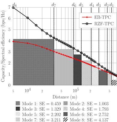
(a) $N_{t}=32,N_{r}=4$

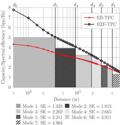
(b) $N_{t}=64,N_{r}=4$

Figure 2: Two examples of designing the RZF-TPC aided and distance-based ACM scheme. The switching thresholds and achievable system throughputs for (a) and (b) are listed in Tables I and II, respectively.

Tables I and II provide two design examples of the RZF-TPC aided and distance-based ACM in conjunction with $(N_{t},N_{r})=(32,4)$ and $(N_{t},N_{r})=(64,4)$, respectively. The RZF-TPC aided and distance-based ACM consists of $K$ ACM modes for providing $K$ data rates. The modulation schemes and code rates are selected from the second generation VersaFEC [41], which is well designed to provide high performance and low latency ACM. The SE of mode $k$, ${\rm SE}_{k}$, is given by

$${\rm SE}_{k}= r_{c}\log_{2}(M)\frac{N}{N+N_{\rm cp}},$$ (76)

where $M$ is the modulation order, $r_{c}$ is the coding rate and the data rate $r_{{\rm pDRA},k}$ per DRA of mode $k$, is given by

$$r_{{\rm pDRA},k}= B_{\rm total}\cdot{\rm SE}_{k},$$ (77)

while the total data rate $r_{{\rm total},k}$ of mode $k$, is given by

$$r_{{\rm total},k}= N_{r}\cdot r_{{\rm pDRA},k}.$$ (78)

More explicitly, Fig. 2(a) illustrates how the $K=8$ ACM modes are designed for the example of Table I. Explicitly, the 8 switching thresholds of Table I are determined so that the SEs of the corresponding ACM modes is just below the SE curve of the RZF-TPC. The $K=7$ ACM modes of Table II are similarly determined, as illustrated in Fig. 2(b). Fig. 2 also confirms that the RZF-TPC aided and distance-based ACM scheme significantly outperforms the EB-TPC aided and distance-based ACM scheme of [19].

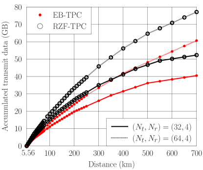
Figure 3: The accumulated transmitted data volume as the function of the distance $d_{b^{*}}^{a^{*}}$ between communicating aircraft $a^{*}$ and $b^{*}$. The distances between the interfering aircraft and the desired receiving aircraft are uniformly distributed within the range of $\big{[}d_{b^{*}}^{a^{*}},~{}D_{\max}\big{]}$, and other system parameters are specified in Table III.

To further compare the RZF-TPC aided and distance-based ACM to the EB-TPC aided and distance-based ACM of [19], we quantitatively calculate their accumulated transmitted data volume $C_{\rm acc}$ that can be exchanged between aircraft $a^{*}$ and aircraft $b^{*}$ both flying at a typical cruising speed of $v=920$ km/h in the opposite direction from the minimum separation distance $d_{\min}=5.56$ km to the maximum communication distance $d_{\max}=740$ km. Let the current distance $d^{a^{*}}_{b^{*}}$ between aircraft $a^{*}$ and aircraft $b^{*}$ be $d^{a^{*}}_{b^{*}}\in\big{(}d_{K-(k^{*}-1)},~{}d_{K-k^{*}}\big{]}$. The accumulated data volume transmitted from $a^{*}$ to $b^{*}$ for $d_{K-(k^{*}-1)}<d^{a^{*}}_{b^{*}}\leq d_{K-k^{*}}$ can be calculated by

$$C_{\rm acc}\big{(}d^{a^{*}}_{b^{*}}\big{)}= \frac{d^{a^{*}}_{b^{*}}-d_{K-k^{*}}}{2v}r_{{\rm total},(K-k^{*})}+\sum\limits_{k=1}^{k^{*}}\frac{d_{K-k}-d_{K-(k-1)}}{2v}r_{{\rm total},(K-(k-1))}.$$ (79)

The accumulated transmitted data volumes expressed in gigabyte (GB) of the RZF-TPC aided and distance-based ACM are compared with the EB-TPC aided and distance-based ACM in Fig. 3, for $(N_{t},N_{r})=(32,4)$ and $(N_{t},N_{r})=(64,4)$. As expected, the achievable accumulated transmitted data volume of the RZF-TPC aided and distance-based ACM is significantly higher than that of the EB-TPC aided and distance-based ACM. In particular, when aircraft $a^{*}$ and $b^{*}$ fly over the communication distance, from $d_{b^{*}}^{a^{*}}=5.56$ km to $d_{b^{*}}^{a^{*}}=740$ km taking a period of about 24 minutes, the RZF-TPC aided and distance-based ACM associated with $(N_{t},N_{r})=(64,4)$ is capable of transmitting a total of about 77 GB of data, while the EB-TPC aided and distance-based ACM with $(N_{t},N_{r})=(64,4)$ is only capable of transmitting about 60 GB of data. Note that (79) can be revised to include any other scenario, by introducing the angle of bearing between two aircraft and their heading direction.

TABLE III: Default system parameters of the simulated AANET.

Number of interference aircraft $A$	4
Number of DRAs $N_{r}$	4
Number of DTAs $N_{t}$	32
Transmit power per antennas $P_{t}$	1 watt
Number of total subcarriers $N$	512
Number of CPs $N_{\rm cp}$	32
Rician factor $K_{\rm Rice}$	5
System bandwidth $B_{\rm total}$	6 MHz
Carrier frequency	5 GHz
Correlation factor between antennas $\rho$	0.1
Noise figure at receiver $F$	4 dB
Distance $d_{b^{*}}^{a^{*}}$ between communicating aircraft $a^{*}$ and $b^{*}$	10 km
Minimum communication distance $D_{\min}$	5.56 km
Maximum communication distance $D_{\max}$	740 km

V Simulation Study

To further evaluate the achievable performance of the proposed RZF-TPC aided and distance-based ACM scheme as well as to investigate the impact of the key system parameters, we consider an AANET consisting of $(A+2)$ aircraft, with two desired communicating aircraft and $A$ interfering aircraft. Each aircraft is equipped with $N_{t}$ DTAs and $N_{r}$ DRAs. The network is allocated $B_{\rm total}=6$ MHz bandwidth at the carrier frequency of 5 GHz. This bandwidth is reused by every aircraft and it is divided into $N=512$ subcarriers. The CP samples are $N_{\rm cp}=32$. The transmit power per antenna is $P_{t}=1$ Watt. The default system parameters are summarized in Table III. Unless otherwise specified, these default parameters are used. The deterministic part of the Rician channel is generated according to the model given in [42], which satisfies $\text{Tr}\left\{\bm{H}_{{\rm d},b}^{a}\big{(}\bm{H}_{{\rm d},b}^{a}\big{)}^{\rm H}\right\}=N_{t}N_{r}$. The scattering component of the Rician channel $\bm{H}_{\text{r},b}^{a}\in\mathbb{C}^{N_{r}\times N_{t}}$ is generated according to (3). As mentioned previously, the DRAs are uncorrelated and, therefore, we have $\bm{R}_{b}=\bm{I}_{N_{r}}$. The spatial correlation matrix of the DTAs is generated according to

$$\bm{R}^{a}\lvert_{[m,n]}= \big{(}\bm{R}^{a}\lvert_{[n,m]}\big{)}^{{\ddagger}}=(t\rho)^{|m-n|},\,1\leq n,m\leq N_{t},$$ (80)

where $(\cdot)^{{\ddagger}}$ denotes the conjugate operator, $t$ is a complex number with $|t|=1$ and $\rho$ is the magnitude of the correlation coefficient that is determined by the antenna element spacing [43].

In the following investigation of the achievable throughput by the RZF-TPC aided and distance-based ACM scheme, ‘Theoretical results’ are the throughputs calculated using (18) using the perfect knowledge of $\left[\bm{M}_{b^{a}}^{a}\right]_{(n_{r},n_{r})}$ and $\left[\bm{M}_{b^{*}}^{a}\right]_{(n_{r}^{*},n_{r}^{*})}$ in (III-C), and the ‘Approximate results’ are the throughputs calculated using (18) with both $\left[\bm{M}_{b^{a}}^{a}\right]_{(n_{r},n_{r})}$ and $\left[\bm{M}_{b^{*}}^{a}\right]_{(n_{r}^{*},n_{r}^{*})}$ substituted by $\left[\bm{M}_{b^{*}}^{a^{*}}\right]_{(n_{r}^{*},n_{r}^{*})}$ in (III-C), while the ‘Simulation results’ represent the Monte-Carlo simulation results. For the EB-TPC aided and distance-based ACM scheme, the ‘Theoretical results’, ‘Approximate results’ and ‘Simulation results’ are defined similarly.

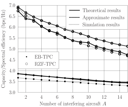
Figure 4: The achievable throughput per DRA as the function of the number of interfering aircraft $A$. The distances between the interfering aircraft and the desired receiving aircraft are uniformly distributed within the range of $\big{[}d_{b^{*}}^{a^{*}},~{}D_{\max}\big{]}$, and the rest of the parameters are specified in Table III.

In Fig. 4, we investigate the achievable throughput per DRA as the function of the number of interfering aircraft $A$. Observe from Fig. 4 that for the RZF-TPC aided and distance-based ACM, the ‘Theoretical results’ are closely matched by the ‘Simulation results’, which indicates that our theoretical analysis presented in Section III is accurate. Furthermore, there is about 0.4 bps/Hz gap between the ‘Theoretical results’ and the ‘Approximate results’. As expected, the achievable throughput degrades as the number of interfering aircraft increases. Moreover, the RZF-TPC aided and distance-based ACM scheme is capable of achieving significantly higher SE than the EB-TPC aided and distance-based ACM scheme.

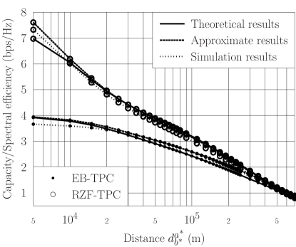
Figure 5: The achievable throughput per DRA as a function of the distance $d_{b^{*}}^{a^{*}}$ between the communicating aircraft $a^{*}$ and $b^{*}$. The distances between the interfering aircraft and the desired receiving aircraft are uniformly distributed within the range of $\big{[}d_{b^{*}}^{a^{*}},~{}D_{\max}\big{]}$, and the rest of the parameters are specified in Table III.

Fig. 5 portrays the achievable throughput per DRA as the function of the distance $d_{b^{*}}^{a^{*}}$ between the communicating aircraft $a^{*}$ and $b^{*}$. Compared to the EB-TPC aided and distance-based ACM, the RZF-TPC aided and distance-based ACM is capable of achieving significantly higher SE, particularly at shorter distances. At the minimum distance of $d_{b^{*}}^{a^{*}}=5.56$ km, the SE improvement is about 3 bps/Hz, but the SE improvement becomes lower as the distance becomes longer. When the distance approaches the maximum communication range of 740 km, both the schemes have a similar SE.

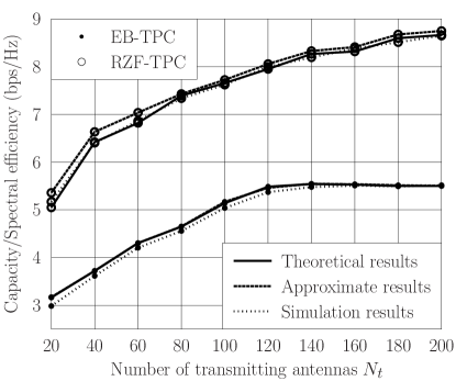
Figure 6: The achievable throughput per DRA as the function of the number of DTAs $N_{t}$. The distances between the interfering aircraft and the desired receiving aircraft are uniformly distributed within the range of $\big{[}d_{b^{*}}^{a^{*}},~{}D_{\max}\big{]}$, and the rest of the parameters are specified in Table III.

Fig. 6 shows the impact of the number of DTAs $N_{t}$ on the achievable throughput. As expected, the achievable throughput increases upon increasing $N_{t}$. Observe from Fig. 6 that for the RZF-TPC aided and distance-based ACM, the ‘Theoretical results’ are closely matched by the ‘Simulation results’, while the ‘Theoretical results’ are closely matched by the ‘Approximate results’, when $N_{t}\geq 80$, but there exists a small gap between the ‘Theoretical results’ and the ‘Approximate result’ for $N_{t}<80$. It can also be seen that the RZF-TPC aided and distance-based ACM achieves approximately 3.0 bps/Hz SE improvement over the EB-TPC aided and distance-based ACM.

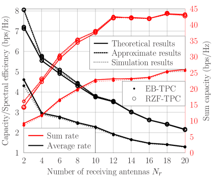
Figure 7: The achievable throughput as the function of the number of DRAs $N_{r}$. The distances between the interfering aircraft and the desired receiving aircraft are uniformly distributed within the range of $\big{[}d_{b^{*}}^{a^{*}},~{}D_{\text{max}}\big{]}$, and the rest of the parameters are specified in Table III.

The impact of the number of DRAs $N_{r}$ on the achievable throughput is studied in Fig. 7, where both the achievable throughput per antenna and the achievable sum rate of all the $N_{r}$ DRAs are plotted. Observe that the achievable throughput per antenna degrades upon increasing $N_{r}$, owing to the increase of the interference amongst the receive antennas. On the other hand, the achievable sum rate increases with $N_{r}$ due to the multiplexing gain. But the sum rate becomes saturated for $N_{r}>12$, because the increase in multiplexing gain is roughly cancelled by the increase of inter-antenna interference. Not surprisingly, the RZF-TPC aided and distance-based ACM significantly outperforms the EB-TPC aided and distance-based ACM.

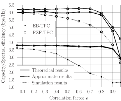
Figure 8: The achievable throughput per DRA as the function of the correlation factor of DTAs $\rho$. The distances between the interfering aircraft and the desired receiving aircraft are uniformly distributed within the range of $\big{[}d_{b^{*}}^{a^{*}},~{}D_{\max}\big{]}$, and the rest of the parameters are specified in Table III.

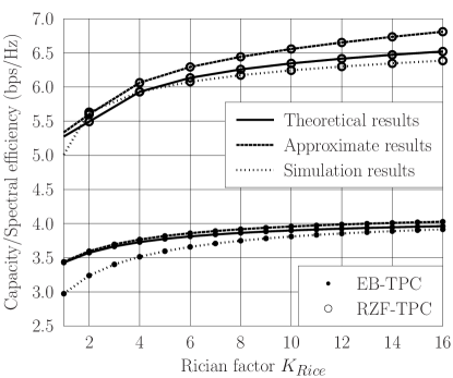
Figure 9: The achievable throughput per DRA as the function of the Rician factor $K_{\rm Rice}$. The distances between the interfering aircraft and the desired receiving aircraft are uniformly distributed within the range of $\big{[}d_{b^{*}}^{a^{*}},~{}D_{\max}\big{]}$, and the rest of the parameters are specified in Table III.

The effect of the correlation factor $\rho$ of the DTAs on the achievable throughput per DRA is shown in Fig. 8. It can be observed that a higher correlation between DTAs results in lower achievable throughput. For the RZF-TPC aided and distance-based ACM, the simulated throughput and the theoretical throughput are close for $\rho\leq 0.4$, but there is a clear performance gap between the ‘Theoretical results’ and the ‘Simulation results’ for $\rho\geq 0.5$. For the EB-TPC aided and distance-based ACM, this performance gap between the ‘Theoretical results’ and the ‘Simulation results’ is even bigger and it exists clearly over the range of $\rho\geq 0.3$. This indicates that for a higher correlation factor $\rho$, the simulated SINR, which is the average over a number of realizations, may deviate considerably from the theoretical SINR, which is the ensemble average. From Fig. 8, it is clear that in addition to achieving a significantly better SE performance, the RZF-TPC aided and distance-based ACM can better deal with the problem caused by strong correlation among the DTAs than the EB-TPC aided and distance-based ACM.

Fig. 9 portrays the impact of the Rician factor $K_{\rm Rice}$ on the achievable throughput per DRA. It can be seen from Fig. 9 that the achievable throughput per DRA increases upon increasing the Rician factor $K_{\rm Rice}$. Furthermore, the SE improvement of the RZF-TPC aided and distance-based ACM over the EB-TPC aided and distance-based ACM also increases with $K_{\rm Rice}$. Specifically, the SE enhancement is about 1.9 bps/Hz at $K_{\rm Rice}=2.0$ and this is increased to about 2.6 bps/Hz for $K_{\rm Rice}=16.0$.

VI Conclusions

A RZF-TCP aided and distance-based ACM scheme has been proposed for large-scale antenna array assisted aeronautical communications. For the design of powerful RZF-TCP, our theoretical contribution has been twofold. For the first time, we have derived the analytical closed-form achievable data rate in the presence of both realistic channel estimation error and co-channel interference. Moreover, we have explicitly derived the optimal regularization parameter that minimizes the mean-square detection error. With the aid of this closed-form data rate metric, we have designed a practical distance-based ACM scheme that switches its coding and modulation mode according to the distance between the communicating aircraft. Our extensive simulation study has quantified the impact of the key system parameters on the achievable throughput of the proposed RZF-TCP aided and distance-based ACM scheme. Our simulation results have confirmed the accuracy of our analytical results. Moreover, both our theoretical analysis and Monte-Carlo simulations have confirmed that the RZF-TCP aided and distance-based ACM scheme substantially outperforms our previous EB-TCP aided and distance-based ACM scheme. In the scenario where two communicating aircraft fly at a typical cruising speed of 920 km/h in opposite direction all the way to the maximum horizon communication distance 740 km, the RZF-TPC aided and distance-based ACM scheme is capable of transmitting about 11.7 GB and 16.5 GB extra data volumes compared to EB-TCP aided and distance-based ACM scheme for the configurations of 32 DTAs/4 DRAs and 64 DTAs/4 DRAs, respectively. This study has therefore offered a practical high-rate, high-SE solution for air-to-air communications.

-A Gallery of Lemmas

Lemma 1 (Matrix inversion lemma I [44])

Given the Hermitian matrix $\bm{A}\in\mathbb{C}^{N\times N}$, vector $\bm{x}\in\mathbb{C}^{N}$ and scalar $\tau\in\mathbb{C}$, if $\bm{A}$ and $\left(\bm{A}+\tau\bm{x}\bm{x}^{\rm H}\right)$ are invertible, the following identity holds

$$\left(\bm{A}+\tau\bm{x}\bm{x}^{\rm H}\right)^{-1}\bm{x}= \frac{\bm{A}^{-1}\bm{x}}{1+\tau\bm{x}^{\rm H}\bm{A}^{-1}\bm{x}}.$$ (81)

Lemma 2 (Matrix inversion lemma II [44])

Given the Hermitian matrix $\bm{A}\in\mathbb{C}^{N\times N}$, vector $\bm{x}\in\mathbb{C}^{N}$ and scalar $\tau\in\mathbb{C}$, if $\bm{A}$ and $\left(\bm{A}+\tau\bm{x}\bm{x}^{\rm H}\right)$ are invertible, the following identity holds

$$\left(\bm{A}+\tau\bm{x}\bm{x}^{\rm H}\right)^{-1}= \bm{A}^{-1}+\frac{\bm{A}^{-1}\tau\bm{x}\bm{x}^{\rm H}\bm{A}^{-1}}{1+\tau\bm{x}^{\rm H}\bm{A}^{-1}\bm{x}}.$$ (82)

Lemma 3 ([19])

Let $\bm{A}\in\mathbb{C}^{N\times N}$ and $\bm{x}\sim\mathcal{CN}\left(\frac{1}{\sqrt{N}}\bm{m},\frac{1}{N}\bm{\Upsilon}\right)$, where $\frac{1}{\sqrt{N}}\bm{m}\in\mathbb{C}^{N}$ and $\frac{1}{N}\bm{\Upsilon}\in\mathbb{C}^{N\times N}$ are the mean vector and the covariance matrix of the random vector $\bm{x}\in\mathbb{C}^{N}$, respectively. Assuming that $\bm{A}$ has a uniformly bounded spectral norm with respect to $N$ and $\bm{x}$ is independent of $\bm{A}$, we have

$$\lim_{N\to\infty}\bm{x}^{\rm H}\bm{A}\bm{x}= \text{Tr}\left\{\left(\frac{1}{N}\bm{M}+\frac{1}{N}\bm{\Upsilon}\right)\bm{A}\right\},$$ (83)

where $\bm{M}=\bm{m}\bm{m}^{\rm H}$.

Lemma 4

Let $\bm{A}\in\mathbb{C}^{N\times N}$, and two independent random vectors $\bm{x}\in\mathbb{C}^{N}$ and $\bm{y}\in\mathbb{C}^{N}$ have the distributions $\bm{x}\sim\mathcal{CN}\left(\frac{1}{\sqrt{N}}\bm{m}_{x},\frac{1}{N}\bm{\Upsilon}_{x}\right)$ and $\bm{y}\sim\mathcal{CN}\left(\frac{1}{\sqrt{N}}\bm{m}_{y},\frac{1}{N}\bm{\Upsilon}_{y}\right)$, where $\frac{1}{\sqrt{N}}\bm{m}_{x}\in\mathbb{C}^{N}$ and $\frac{1}{\sqrt{N}}\bm{m}_{y}\in\mathbb{C}^{N}$ are the mean vectors, while $\frac{1}{N}\bm{\Upsilon}_{x}\in\mathbb{C}^{N\times N}$ and $\frac{1}{N}\bm{\Upsilon}_{y}\in\mathbb{C}^{N\times N}$ are the covariance matrices of $\bm{x}$ and $\bm{y}$, respectively. Assuming that $\bm{A}$ has a uniformly bounded spectral norm with respect to $N$, and $\bm{x}$ and $\bm{y}$ are independent of $\bm{A}$, we have

$$\lim_{N\to\infty}\bm{x}^{\rm H}\bm{A}\bm{y}= \text{Tr}\left\{\frac{1}{N}\bm{M}_{xy}\bm{A}\right\},$$ (84)

where $\bm{M}_{xy}=\bm{m}_{x}\bm{m}_{y}^{\rm H}$.

Proof 1

Let $\bm{z}_{x}=\sqrt{N}\bm{x}-\bm{m}$. Since $\bm{x}\sim\mathcal{CN}\left(\frac{1}{\sqrt{N}}\bm{m}_{x},\frac{1}{N}\bm{\Upsilon}_{x}\right)$, $\bm{z}_{x}\sim\mathcal{CN}\left(\bm{0}_{N},\bm{\Upsilon}_{x}\right)$. Let $\bm{z}_{y}=\sqrt{N}\bm{y}-\bm{m}$. As $\bm{y}\sim\mathcal{CN}\left(\frac{1}{\sqrt{N}}\bm{m}_{y},\frac{1}{N}\bm{\Upsilon}_{y}\right)$, $\bm{z}_{x}\sim\mathcal{CN}\left(\bm{0}_{N},\bm{\Upsilon}_{y}\right)$. Furthermore,

$$\bm{x}^{\rm H}\bm{A}\bm{y}= \left(\frac{1}{\sqrt{N}}\bm{m}_{x}+\frac{1}{\sqrt{N}}\bm{z}_{x}\right)^{\rm H}\bm{A}\left(\frac{1}{\sqrt{N}}\bm{m}_{y}+\frac{1}{\sqrt{N}}\bm{z}_{y}\right)$$

$$= \frac{1}{N}\bm{m}_{x}^{\rm H}\bm{A}\bm{m}_{y}+\frac{1}{N}\bm{z}_{x}^{\rm H}\bm{A}\bm{z}_{y}+\frac{1}{N}\bm{m}_{x}^{\rm H}\bm{A}\bm{z}_{y}+\frac{1}{N}\bm{z}_{x}^{\rm H}\bm{A}\bm{m}_{y}.$$ (85)

Since $\bm{z}_{x}\sim\mathcal{CN}\left(\bm{0}_{N},\bm{\Upsilon}_{x}\right)$ and $\bm{z}_{y}\sim\mathcal{CN}\left(\bm{0}_{N},\bm{\Upsilon}_{y}\right)$, $\bm{z}_{x}$ and $\bm{z}_{y}$ do not depend on $\bm{m}_{x}$ and $\bm{m}_{y}$. According to Lemma 1 of [37], we have

$$\lim\limits_{N\to\infty}\frac{\bm{m}_{x}^{\rm H}\bm{A}\bm{z}_{y}}{N}= 0,$$ (86)

$$\lim\limits_{N\to\infty}\frac{\bm{z}_{x}^{\rm H}\bm{A}\bm{m}_{y}}{N}= 0.$$ (87)

Since $\bm{z}_{x}$ and $\bm{z}_{y}$ are independent, according to the trace lemma of [45], we have

$$\lim\limits_{N\to\infty}\frac{1}{N}\bm{z}_{x}^{\rm H}\bm{A}\bm{z}_{y}=0.$$ (88)

Furthermore,

$$\frac{1}{N}\bm{m}_{x}^{\rm H}\bm{A}\bm{m}_{y}=\text{Tr}\left\{\frac{1}{N}\bm{A}\bm{M}_{xy}\right\}.$$ (89)

Taking the limit $N\to\infty$ as well as substituting (86) to (89) into (1) results in (84).

-B Derivation of the Optimal Regularization Parameter

Because the term $\mathcal{E}\bigg{\{}\sum\limits_{a=1}^{A}\Big{\|}\frac{1}{N_{t}}\sqrt{\frac{P_{r,b^{*}}^{a}}{P_{r,b^{*}}^{a^{*}}}}\bm{H}_{b^{*}}^{a}\bm{V}_{b^{a}}^{a}\bm{X}^{a}\Big{\|}^{2}+\Big{\|}\frac{1}{N_{t}\sqrt{P_{r,b^{*}}^{a^{*}}}}\bm{W}_{b^{*}}\Big{\|}^{2}\bigg{\}}$ is independent of $\xi_{b^{*}}^{a^{*}}$,

$$\frac{d\,\mathcal{J}\big{(}\xi_{b^{*}}^{a^{*}}\big{)}}{d\,\xi_{b^{*}}^{a^{*}}}= \mathcal{E}\Bigg{\{}\bigg{(}\frac{1}{N_{t}}\bm{H}_{b^{*}}^{a^{*}}\bm{V}_{b^{*}}^{a^{*}}\bm{X}^{a^{*}}-\bm{X}^{a^{*}}\bigg{)}^{\rm H}\frac{d\,\big{(}\frac{1}{N_{t}}\bm{H}_{b^{*}}^{a^{*}}\bm{V}_{b^{*}}^{a^{*}}\bm{X}^{a^{*}}-\bm{X}^{a^{*}}\big{)}}{d\,\xi_{b^{*}}^{a^{*}}}$$

$$+\frac{d\,\big{(}\frac{1}{N_{t}}\bm{H}_{b^{*}}^{a^{*}}\bm{V}_{b^{*}}^{a^{*}}\bm{X}^{a^{*}}-\bm{X}^{a^{*}}\big{)}^{\rm H}}{d\,\xi_{b^{*}}^{a^{*}}}\Big{(}\frac{1}{N_{t}}\bm{H}_{b^{*}}^{a^{*}}\bm{V}_{b^{*}}^{a^{*}}\bm{X}^{a^{*}}-\bm{X}^{a^{*}}\Big{)}\Bigg{\}}$$

$$=\mathcal{E}\bigg{\{}\bigg{(}\frac{1}{N_{t}}\bm{H}_{b^{*}}^{a^{*}}\bm{V}_{b^{*}}^{a^{*}}\bm{X}^{a^{*}}-\bm{X}^{a^{*}}\bigg{)}^{\rm H}\bigg{(}-\frac{1}{N_{t}}\bm{H}_{b^{*}}^{a^{*}}\Big{(}\big{(}\bm{\Upsilon}_{b^{*}}^{a^{*}}\big{)}^{2}\big{(}\widehat{\bm{H}}_{b^{*}}^{a^{*}}\big{)}^{\rm H}\Big{)}\bm{X}^{a^{*}}\bigg{)}$$

$$+\bigg{(}-\frac{1}{N_{t}}\bm{H}_{b^{*}}^{a^{*}}\Big{(}\big{(}\bm{\Upsilon}_{b^{*}}^{a^{*}}\big{)}^{2}\big{(}\widehat{\bm{H}}_{b^{*}}^{a^{*}}\big{)}^{\rm H}\Big{)}\bm{X}^{a^{*}}\bigg{)}^{\rm H}\bigg{(}\frac{1}{N_{t}}\bm{H}_{b^{*}}^{a^{*}}\bm{V}_{b^{*}}^{a^{*}}\bm{X}^{a^{*}}-\bm{X}^{a^{*}}\bigg{)}\bigg{\}}$$

$$=\mathcal{E}\bigg{\{}\!\!-\!\frac{1}{N_{t}^{2}}\text{Tr}\Big{\{}\!E_{\rm s}\widehat{\bm{H}}_{b^{*}}^{a^{*}}\bm{\Upsilon}_{b^{*}}^{a^{*}}\big{(}\bm{H}_{b^{*}}^{a^{*}}\big{)}^{\rm H}\bm{H}_{b^{*}}^{a^{*}}\big{(}\bm{\Upsilon}_{b^{*}}^{a^{*}}\big{)}^{2}\big{(}\widehat{\bm{H}}_{b^{*}}^{a^{*}}\big{)}^{\rm H}\!\Big{\}}\!+\!\frac{1}{N_{t}}\text{Tr}\Big{\{}\!E_{\rm s}\bm{H}_{b^{*}}^{a^{*}}\big{(}\bm{\Upsilon}_{b^{*}}^{a^{*}}\big{)}^{2}\!\big{(}\widehat{\bm{H}}_{b^{*}}^{a^{*}}\big{)}^{\rm H}\!\Big{\}}$$

$$\!\!-\!\frac{1}{N_{t}^{2}}\text{Tr}\Big{\{}\!E_{\rm s}\widehat{\bm{H}}_{b^{*}}^{a^{*}}\big{(}\bm{\Upsilon}_{b^{*}}^{a^{*}}\big{)}^{2}\big{(}\bm{H}_{b^{*}}^{a^{*}}\big{)}^{\rm H}\bm{H}_{b^{*}}^{a^{*}}\bm{\Upsilon}_{b^{*}}^{a^{*}}\big{(}\widehat{\bm{H}}_{b^{*}}^{a^{*}}\big{)}^{\rm H}\!\Big{\}}\!+\!\frac{1}{N_{t}}\text{Tr}\Big{\{}\!E_{\rm s}\widehat{\bm{H}}_{b^{*}}^{a^{*}}\big{(}\bm{\Upsilon}_{b^{*}}^{a^{*}}\big{)}^{2}\big{(}\bm{H}_{b^{*}}^{a^{*}}\big{)}^{\rm H}\!\Big{\}}\!\!\bigg{\}}\!,\!$$ (90)

where $E_{\rm s}=\mathcal{E}\big{\{}\big{|}X_{n_{r}}^{a^{*}}\big{|}^{2}\big{\}}$, $1\leq n_{r}\leq N_{r}$. Setting $\frac{d\,\mathcal{J}\big{(}\xi_{b^{*}}^{a^{*}}\big{)}}{d\,\xi_{b^{*}}^{a^{*}}}=0$ and followed by some further operations yields

$$\text{Tr}\bigg{\{}\bigg{(}\frac{1}{N_{t}}\widetilde{\bm{\Xi}}_{b^{*}}^{a^{*}}-\xi_{b^{*}}^{a^{*}}\bm{I}_{N_{t}}\bigg{)}\bm{\Upsilon}_{b^{*}}^{a^{*}}\big{(}\widehat{\bm{H}}_{b^{*}}^{a^{*}}\big{)}^{\rm H}\widehat{\bm{H}}_{b^{*}}^{a^{*}}\big{(}\bm{\Upsilon}_{b^{*}}^{a^{*}}\big{)}^{2}\bigg{\}}=0,$$ (91)

where $\widetilde{\bm{\Xi}}_{b^{*}}^{a^{*}}=\text{diag}\big{\{}\widetilde{\varphi}_{1},\cdots,\widetilde{\varphi}_{N_{t}}\big{\}}$. This proves that (73) is an optimal regularization parameter.

References

• [1] J. Zhang, et al., “A survey of aeronautical ad-hoc networking,” submitted to IEEE Commun. Surveys & Tutorials, 2017.
• [2] A. Jahn, et al., “Evolution of aeronautical communications for personal and multimedia services,” IEEE Commun. Mag., vol. 41, no. 7, pp. 36–43, Jul. 2003.
• [3] Q. Vey, A. Pirovano, J. Radzik, and F. Garcia, “Aeronautical ad hoc network for civil aviation,” in Proc. 6th Int. Workshop Commun. Tech. for Vehicles, Nets4Cars/Nets4Trains/Nets4Aircraft 2014 (Offenburg, Germany), May 6-7, 2014, pp. 81–93.
• [4] M. Schnell, U. Epple, D. Shutin, and N. Schneckenburger, “LDACS: future aeronautical communications for air-traffic management,” IEEE Commun. Mag., vol. 52, no. 5, pp. 104–110, May 2014.
• [5] R. Jain, F. Templin, and K.-S. Yin, “Analysis of L-band digital aeronautical communication systems: L-DACS1 and L-DACS2,” in Proc. 2011 IEEE Aerospace Conf. (Big Sky, Montana), Mar. 5-12, 2011, pp. 1–10.
• [6] G. Bartoli, R. Fantacci, and D. Marabissi, “AeroMACS: a new perspective for mobile airport communications and services,” IEEE Wirel. Commun., vol. 20, no. 6, pp. 44–50, Dec. 2013.
• [7] T. Gräupl, M. Ehammer, and S. Zwettler, “L-DACS1 air-to-air data-link protocol design and performance,” in Proc. ICNS 2011 (Herndon, VA), May 10-12, 2011, pp. 1–10.
• [8] B. Haind, “An independent technology assessment for a future aeronautical communication system based on potential systems like B-VHF,” in Proc. DASC 2007 (Dallas, TX), Oct. 21-25, 2007, pp. 4.D.6-1–4.D.6-12.
• [9] D. Stacey, Aeronautical Radio Communication Systems and Networks. John Wiley & Sons: Chichester, UK, 2008.
• [10] E. G. Larsson, O. Edfors, F. Tufvesson, and T. L. Marzetta, “Massive MIMO for next generation wireless systems,” IEEE Commun., vol. 52, no. 2, pp. 186–195, Feb. 2014.
• [11] A. J. Goldsmith and S.-G. Chua, “Adaptive coded modulation for fading channels,” IEEE Trans. Commun., vol. 46, no. 5, pp. 595–602, May 1998.
• [12] L. Hanzo, C. H. Wong, and M. S. Yee, Adaptive Wireless Transceivers: Turbo-Coded, Turbo-Equalised and Space-Time Coded TDMA, CDMA, MC-CDMA and OFDM Systems. John Wiley: New York, USA, 2002.
• [13] S. Zhou and G. B. Giannakis, “Adaptive modulation for multiantenna transmissions with channel mean feedback,” IEEE Trans. Wirel. Commun., vol. 3, no. 5, pp. 1626–1636, Sep. 2004.
• [14] S. Zhou and G. B. Giannakis, “How accurate channel prediction needs to be for transmit-beamforming with adaptive modulation over Rayleigh MIMO channels?” IEEE Trans. Wirel. Commun., vol. 3, no. 4, pp. 1285–1294, Jul. 2004.
• [15] M. Taki, M. Rezaee, and M. Guillaud, “Adaptive modulation and coding for interference alignment with imperfect CSIT,” IEEE Trans. Wirel. Commun., vol. 13, no. 9, pp. 5264–5273, Sep. 2014.
• [16] L. Hanzo, S. X. Ng, T. Keller, W. Webb, Quadrature Amplitude Modulation: From Basics to Adaptive Trellis-Coded, Turbo-Equalised and Space-Time Coded OFDM, CDMA and MC-CDMA Systems (Second Edition). Wiley-IEEE Press: New York, USA, 2004.
• [17] E. Haas, “Aeronautical channel modeling,” IEEE Trans. Veh. Techno., vol. 51, no. 2, pp. 254–264, Mar. 2002.
• [18] Y. S. Meng and Y. H. Lee, “Measurements and characterizations of air-to-ground channel over sea surface at C-band with low airborne altitudes,” IEEE Trans. Veh. Techno., vol. 60, no. 4, pp. 1943–1948, May 2011.
• [19] J. Zhang, et al., “Adaptive coding and modulation for large-scale antenna array based aeronautical communications in the presence of co-channel interference,” IEEE Trans. Wirel. Commun., vol. 17, no. 2, pp. 1343–1357, Feb. 2018.
• [20] A. Wiesel, Y. C.  Eldar, and S. Shamai, “Zero-forcing precoding and generalized inverses,” IEEE Trans. Signal Process., vol. 56, no. 9, pp. 4409–4418, Sep. 2008.
• [21] H. Tataria, P. J. Smith, L. J. Greenstein, and P. A. Dmochowski , “Zero-forcing precoding performance in multiuser MIMO systems with heterogeneous Ricean fading,” IEEE Wirel. Commun. Lett., vol. 6, no. 1, pp. 74–77, Feb. 2017.
• [22] C. B. Peel, B. M. Hochwald, and A. L. Swindlehurst, “A vector-perturbation technique for near-capacity multiantenna multiuser communication–Part I: channel inversion and regularization,” IEEE Trans. Commun., vol. 53, no. 1, pp. 195–202, Jan. 2005.
• [23] J. Zhang, et al., “Large system analysis of cooperative multi-cell downlink transmission via regularized channel inversion with imperfect CSIT,” IEEE Trans. Wirel. Commun., vol. 12, no. 10, pp. 4801–4813, Oct. 2013.
• [24] J. Hoydis, S. Ten Brink, and M. Debbah, “Massive MIMO in the UL/DL of cellular networks: How many antennas do we need?” IEEE J. Sel. Areas Commun., vol. 31, no. 2, pp. 160–171, Feb. 2013.
• [25] H. Tataria, et al.,“Performance and analysis of downlink multiuser MIMO systems with regularized zero-forcing precoding in Ricean fading channels,” in Proc. ICC 2016 (Kuala Lumpur, Malaysia), May 22-27, 2016, pp. 1–7.
• [26] H. Falconet, L. Sanguinetti, A. Kammoun, and M. Debbah,“Asymptotic analysis of downlink MISO systems over Rician fading channels,” in Proc. ICASSP 2016 (Shanghai, China), Mar. 20-25, 2016, pp. 3926–3930.
• [27] L. Sanguinetti, A. Kammoun, and M. Debbah, “Asymptotic analysis of multicell massive MIMO over Rician fading channels,” in Proc. ICASSP 2017 (New Orleans, USA), Mar. 5-9, 2017, pp. 3539–3543.
• [28] J. Zhang, et al., “Pilot contamination elimination for large-scale multiple-antenna aided OFDM systems,” IEEE J. Sel. Topics Signal Process., vol. 8, no. 5, pp. 759–772, Oct. 2014.
• [29] X. Guo, et al., “Optimal pilot design for pilot contamination elimination/reduction in large-scale multiple-antenna aided OFDM systems,” IEEE Trans. Wirel. Commun., vol. 15, no. 11, pp. 7229–7243, Nov. 2016.
• [30] P. A. Bello, “Aeronautical channel characterization,” IEEE Trans. Commun., vol. 21, no. 5, pp. 548–563, May 1973.
• [31] M. Walter and M. Schnell, “The Doppler delay characteristic of the aeronautical scatter channel,” in Proc. VTC-Fall 2011 (San Francisco, USA), Sept. 5-8 , 2011, pp. 1–5.
• [32] K. Kim, J. Lee, and H. Liu, “Spatial-correlation-based antenna grouping for MIMO systems,” IEEE Trans. Veh. Techno., vol. 59, no. 6, pp. 2898–2905, Jul. 2010.
• [33] H. Tataria, P. J. Smith, L. J. Greenstein, and P. A. Dmochowski , “Impact of line-of-sight and unequal spatial correlation on uplink MU-MIMO systems,” IEEE Wirel. Commun. Lett., vol. 6, no. 5, pp. 634–637, Oct. 2017.
• [34] J. D. Parsons, The Mobile Radio Propagation Channel (2nd Edition). John Wiley & Sons: Chichester, UK, 2000.
• [35] S. Gligorevic, “Airport surface propagation channel in the C-Band: measurements and modeling,” IEEE Trans. Antennas Propag., vol. 61, no. 9, pp. 4792-–4802, Sep. 2013.
• [36] S. M. Kay, Fundamentals of Statistical Signal Processing: Estimation Theory. Prentice-Hall: Upper Saddle River, 2003.
• [37] F. Fernandes, A. Ashikhmin, and T. L. Marzetta, “Inter-cell interference in noncooperative TDD large scale antenna systems,” IEEE J. Sel. Areas Commun., vol. 31, no. 2, pp. 192–201, Feb. 2013.
• [38] W. Hachem, P. Loubaton, and J. Najim, “Deterministic equivalents for certain functionals of large random matrices,” Ann. Appl. Prob., vol. 17, no. 3, pp. 875–930, May 2007.
• [39] W. Hachem, P. Loubaton, J. Najim, and P. Vallet, “On bilinear forms based on the resolvent of large random matrices,” Ann. Inst. H. Poincaré Probab. Statist., vol. 49, no. 1, pp.  36-63, Feb. 2013.
• [40] M. E. Ismail and D. H. Kelker, “Special functions, Stieltjes transforms and infinite divisibility,” SIAM J. Mathematical Analysis, vol. 10, no. 5, pp. 884–901, May 1979.
• [41] Comtech EF Data, “CDM-625A Advanced Satellite Modem,” https://www.comtechefdata.com/files/datasheets/ds-cdm625A.pdf, Accessed on November 11th, 2017, [[Online]. Available].
• [42] S. Jin, M. R. McKay, K. K. Wong and X. Li, “Low-SNR capacity of multiple-antenna systems with statistical channel-state information,” IEEE Trans. Veh. Techno., vol. 59, no. 6, pp. 2874–2884, Jul. 2010.
• [43] B. Lee, J. Choi, J.-Y. Seol, D. J. Love, and B. Shim, “Antenna grouping based feedback compression for FDD-based massive MIMO systems,” IEEE Trans. Commun., vol. 63, no. 9, pp. 3261–3274, Sep. 2015.
• [44] J. W. Silverstein and Z. D. Bai, “On the empirical distribution of eigenvalues of a class of large dimensional random matrices,” J. Multivariate analysis, vol. 54, no. 2, pp. 175–192, Aug. 1995.
• [45] J. Hoydis, Random Matrix Theory for Advanced Communication Systems. Ph.D. dissertation, Supélec, 2012.