Tensor Methods for Additive Index Models under Discordance and Heterogeneity

Abstract

Motivated by the sampling problems and heterogeneity issues common in high-dimensional big datasets, we consider a class of discordant additive index models. We propose method of moments based procedures for estimating the indices of such discordant additive index models in both low and high-dimensional settings. Our estimators are based on factorizing certain moment tensors and are also applicable in the overcomplete setting, where the number of indices is more than the dimensionality of the datasets. Furthermore, we provide rates of convergence of our estimator in both high and low-dimensional setting. Establishing such results requires deriving tensor operator norm concentration inequalities that might be of independent interest. Finally, we provide simulation results supporting our theory. Our contributions extend the applicability of tensor methods for novel models in addition to making progress on understanding theoretical properties of such tensor methods.

1 Introduction

High-dimensional big datasets are typically collected by aggregating information from a variety of sources. Such diverse sources of data, invariably cause sampling challenges and heterogeneity issues (Fan et al., 2014). Motivated by these concerns, in this work, we consider a class of additive index models (AIMs) described as follows. Given the covariate $X$, we let $\mathcal{Z}=\{Z_{j}=f_{j}(\langle X,\beta^{*}_{j}\rangle)+\epsilon_{j}\}_{j\in[k]}$ be an underlying set of latent models. That is, $\mathcal{Z}$ is an unordered collection of the responses of $k$ single index models (SIMs), that are unobservable. Here $\{\epsilon_{j}\}_{j\in[k]}$ are exogenous noise. Moreover, based on $\mathcal{Z}$, the observed response $Y$ is given by a real-valued function $h:\mathcal{Z}\to\mathbb{R}$ such that

$${\mathbb{E}}(Y|X)={\mathbb{E}}(h(\mathcal{Z})|X)=g_{1}(\langle X,\beta^{*}_{1}\rangle)+g_{2}(\langle X,\beta^{*}_{2}\rangle)+\ldots+g_{k}(\langle X,\beta^{*}_{k}\rangle).$$ (1)

Here, the functions $g$ actually depend on the choice of $h$ and $f$. To avoid notational clutter, we just use $g$ to denote it. In addition, we note that the function $h$ can be a random function that is independent of $\mathcal{Z}$. We call this model as discordant additive index model (DAIM), as the response $Y$ depends on the latent set $\mathcal{Z}$. We allow the model to be overcomplete, where the number of index models, $k$, is larger than the dimensionality $d$. Given $n$ i.i.d. observations $\{(X^{(i)},h(\mathcal{Z}^{(i)}))\}_{i\in[n]}$ of the DAIM in (1), our goal is to estimate the parametric components $\{\beta^{*}_{j}\}_{j\in[k]}$.

Our estimators are based on method of moments approach and involve factorizing higher-order moment tensors. The corresponding second-order analogue, called as principal component analysis, has been leveraged widely for estimation in several statistical problems, for example, factor modeling, dimensionality reduction, estimation in mixture models and community detection. Furthermore, inferential and computational properties of such estimators for the above problems are relatively well understood. It is worth noting that establishing operator norm bounds for certain random matrices played a crucial part in deriving such results. We refer the reader to Fan et al. (2018) for a detailed survey of such results. In comparison, for the higher-order case, both the methodology and the theory of tensor factorization approaches are still in its infancy. In this paper, we adopt the tensor decomposition framework (Anandkumar et al., 2014a, b; Sun et al., 2017) for estimating the parameters of the DAIM in (1), and also derive operator norm bounds for the decomposed moment tensors, thereby making progress towards understanding theoretical properties of higher-order decompositions and widening their applicability.

We now provide two concrete instantiations of the DAIM by appropriately defining the sampling function $h$ and motivate their applications. A canonical example of DAIM are the mixture models used to model heterogeneity (McLachlan and Peel, 2004; Fan et al., 2014; Städler et al., 2010). In this setting, only one element of the latent $\mathcal{Z}$ is observed. That is, $h(\mathcal{Z})$ is assumed to be a random function that picks element $Z_{j}$ with probability $\pi_{j}$ where $\sum_{j\in[k]}\pi_{j}=1$. Hence the observation is given by $Y=h(\mathcal{Z})=Z_{j}$ with probability $\pi_{j}$. Again, it is easy to see that the model is an instantiation of the DAIM posited in (1), with appropriately defined $g$ functions. Correspondingly in the sample setting, given $n$ i.i.d samples $X^{(i)}\in\mathbb{R}^{d}$ and the matrix $Z_{ij}\in\mathbb{R}^{k\times n}$, for each column, one of the $k$ entries is observed and the probability of observing the $j$-th entry is given by $\pi_{j}$ independently for all columns. From a practical perspective, heterogenous data is ubiquitous. For example, in genomics and neuroscience, the occurrences of systematic biases is natural due to the data being combined from multiple sources. Similarly in financial econometrics, the sources of data available includes stocks, trading data and unstructured text from news and blog sources. In these situations, failure to acknowledge data heterogeneity leads to wrong inferences (Fan et al., 2014). Furthermore, in practice the non-parametric component can be misspeficied and the number of components, $k$, can be greater than the dimensionality of the dataset causing more challenges for estimation.

Yet another example of the DAIM is the problem of correspondence retrieval proposed recently in Andoni et al. (2017). Here, the correspondence between the model under consideration ($\beta_{j}$) and the actual responses at hand ($Z_{j}$) is unobserved. Instead, we observe say the average (or sum) of the responses, $k^{-1}\sum_{j\in[k]}Z_{j}$. It is clear that if the sampling function is taken as $h(\mathcal{Z})=k^{-1}\sum_{j\in[k]}Z_{j}=k^{-1}\sum_{j\in[k]}[f_{j}(\langle X,\beta^{*}_{j}\rangle)+\epsilon_{j}]$, the model is an instantiation of the DAIM posited in (1), with appropriately defined $g$ functions that depend on the corresponding $f$ functions. In the sample setting, given $n$ i.i.d. samples $X^{(i)}\in\mathbb{R}^{d}$, consider the matrix $Z\in\mathbb{R}^{k\times n}$ where each $Z_{ij}=f_{j}(\langle X^{(i)},\beta_{j}\rangle)+\epsilon_{j}^{(i)}$. Let $\{\mathcal{Z}^{(i)}\}_{i\in[n]}$ be $n$ i.i.d. sets of latent observations, where $\mathcal{Z}^{(i)}=\{Z_{ij},j\in[k]\}$. Then the $i^{th}$ responses $Y_{i}$ is given by $h(\mathcal{Z}_{i})=k^{-1}\sum_{j\in[k]}Z_{ij}$. That is, we do not observe the matrix $Z$ which has the correspondence information in the sample setting. Instead, we observe discordant observations of the form $h(\mathcal{Z}^{(i)})$, which obscures the correspondence information. From a practical point of view, such a lack of correspondence occurs in several situations. For example in high-dimensional nonlinear multi-task learning models (Yang et al., 2009), due to privacy or record linkage issues, one might not observe the correspondence between the response and the covariates of the different models. Furthermore, our models also are applicable to nonlinear compressed sensing in the discordant setting which has wide applications as described in (Unnikrishnan et al., 2015). Similar to the previous example, model misspecification and having a large number of components, $k$, cause significant challenges for estimation.

Contributions: Motivated by the above discussion, we focus on the task of estimating the parametric components of the DAIM, while being agnostic to the nonparametric components. First, it is worth noting that likelihood/least-squares based approaches depend on the specification of the nonparametric components and is not agnostic to them. Hence, we propose to use a higher-order moment decomposition based procedure to provably recover the parametric components with unknown nonparametric components. Under a Gaussian design assumption on the covariate and under mild regularity assumptions on the unknown nonparametric components (the specific details are provided in §2.1), we provide polynomial-time computable estimators that achieve optimal statistical rates, in both low and high-dimensional settings, with sufficiently large number of samples. The statistical rates for our estimator are established based on obtaining novel concentration inequalities in tensor operator norm for the considered moment tensors, which might be of independent interest. Finally, from a practical point of view, our estimator for the parametric components could also be used as initializers for alternating minimization algorithms (e.g., the EM algorithm) to estimate the nonparametric components efficiently.

Notations: We denote by $[n]$ the set of integers $\{1,\ldots,n\}$. Furthermore, for a vector $u\in\mathbb{R}^{d}$ and an index set $F\subseteq[d]$, the truncation of $u$ with respect to the set $F$, denoted as $\vartheta_{F}(u)$, is defined coordinate-wise as

$$\left[\vartheta_{F}(u)\right]_{i}=\begin{cases}u_{i}&\text{if}~{}i\in F\\ 0&\text{otherwise.}\end{cases}$$

We also use the notation $\vartheta_{s}(u)$ to denote the case where $F$ consists of the top-$s$ entries of $u$ in absolute value. We denote an $\ell$-th order symmetric tensor by $A\in\mathbb{R}^{d\otimes\ell}$. Recall that a tensor is symmetric if $A_{j_{1}j_{2}\cdots j_{\ell}}=A_{j_{\sigma(1)}j_{\sigma(2)}\cdots j_{\sigma(\ell)}}$, for every permutation $\sigma$ of the indices. For a given vector $u\in\mathbb{R}^{d}$, we define the $\ell$-th order rank-1 tensor formed from $u$ as $u^{\otimes\ell}$. Similarly, for a given set of $k$ vectors $u^{(1)},\ldots,u^{(\ell)}\in\mathbb{R}^{d}$, the rank-1 tensor formed by taking the outer product of them is given by $u^{(1)}\otimes u^{(2)}\otimes\cdots\otimes u^{(\ell)}$. In addition, let $A$ and $B$ be two $\ell$-th order tensors, we define the inner product between $A$ and $B$ as $\langle A,B\rangle=\sum_{j_{1}=1}^{d}\cdots\sum_{j_{\ell}=1}^{d}A_{j_{1}j_{2}\ldots j_{\ell}}\cdot B_{j_{1}j_{2}\ldots j_{k}}$. Furthermore, for any $A\in\mathbb{R}^{d\otimes\ell}$ and $p\in(0,\infty)$, we define the element-wise $\ell_{p}$-norm as $\|A\|_{p}=(\sum_{j_{1},\ldots,j_{\ell}=1}^{d}|A_{j_{1}j_{2}\cdots j_{\ell}}|^{p})^{1/p}$. Note that this generalizes the standard element-wise $\ell_{p}$-norm of a vector. We also denote the $\ell$-th order polynomial form of the tensor $A$ as $A(u^{(1)},\ldots,u^{(\ell)})=\bigl{\langle}A,u^{(1)}\otimes u^{(2)}\otimes\cdots\otimes u^{(\ell)}\bigr{\rangle}$. Note that here $A(u^{(1)},\ldots,u^{(\ell)})$ is a function of $\{u^{(j)}\}_{j\in[\ell]}$. The operator norm of a tensor $A$ is then defined as

$$\|A\|_{\operatorname{{\rm op}}}=\sup\bigl{\{}\bigl{|}A(u^{(1)},\ldots,u^{(\ell)})\bigr{|}\colon u^{(1)},u^{(2)},\ldots,u^{(\ell)}\in\mathbb{S}^{d-1}\bigr{\}},$$ (2)

where $\mathbb{S}^{d-1}=\{u\in\mathbb{R}^{d}\colon\|u\|_{2}=1\}$ is the unit sphere in $\mathbb{R}^{d}$. Note that when the tensor is symmetric, the operator norm can alternatively be calculated as $\|A\|_{\operatorname{{\rm op}}}=\sup\bigl{\{}\bigl{|}A(u,\ldots,u)\bigr{|}\colon u\in\mathbb{S}^{d-1}\bigr{\}}$. Note that when $\ell=2$, we recover the matrix operator norm. We also define the sparse symmetric tensor operator norm, for some $1\leq r\leq d$, as

$$\|A\|_{\operatorname{{\rm op}},r}=\sup\bigl{\{}\bigl{|}A(u,\ldots,u)\bigr{|}\colon u\in\mathbb{S}^{d-1}~{}\text{and}~{}\|u\|_{0}\leq r\bigr{\}}.$$ (3)

For a $(\ell-1)$-th order symmetric tensor-valued function $A_{\ell-1}(a):\mathbb{R}^{d}\mapsto\mathbb{R}^{d\otimes(\ell-1)}$, its derivative is given by an $\ell$-th order symmetric tensor $\nabla_{a}A_{\ell-1}(a)$ which is defined entry wise as $[\nabla_{a}A_{\ell-1}(a)]_{i_{1},\ldots,i_{\ell}}=\partial[A_{\ell-1}(a)]_{i_{1},\ldots,i_{(\ell-1)}}/\partial a_{i_{\ell}}$. Finally, for a function $f(a):\mathbb{R}^{d}\to\mathbb{R}$, its $\ell$-th derivative is denoted as $f^{(\ell)}(a)$. We end this section by describing the format of the paper. In §2, we precisely define the class of DAIM that we consider and outline our estimator which is based on decomposing higher-order moment tensors. In §3, we present our main results regarding the rate of convergence of our estimators in both low and high-dimensional setting, that involve obtaining tensor operator norm concentration results. The proofs are relegated to §A.

2 Model Definition and Estimation

We now introduce the precise definitions of the models that we consider in this work and outline our moment-based estimation procedure. As discussed in §1, our primary motivation for the DAIM in (1) is based on handling discordance and heterogeneity in the high-dimensional big data settings. In the following, we define two instantiations of the DAIM and propose the corresponding estimation procedures. We first introduce the discordant single index models, which is a special case of DAIM under discordance.

Definition 1 (Discordant SIMs).

We assume that there are $k$ unordered latent single index models denoted by $\mathcal{Z}=\{Z_{j}=f_{j}(\langle\beta_{j}^{*},X\rangle,\epsilon_{j})\}_{j\in[k]}$. Here $X\in\mathbb{R}^{d}$ is the covariate, $\{\epsilon_{j}\}_{j\in[k]}\subseteq\mathbb{R}$ are the random noise independent of $X$, and $\{f_{j}\colon\mathbb{R}^{2}\rightarrow\mathbb{R}\}_{j\in[k]}$ are unknown link functions. Based on $\mathcal{Z}$, we observe the response variable $Y=h_{1}(\mathcal{Z})=k^{-1}\sum_{j\in[k]}Z_{j}$.

In this model, the set of responses $\mathcal{Z}$ is latent and the response observed is given by the average function $h_{1}(\mathcal{Z})$. In addition, since the norm of $\beta^{*}_{j}$ can be absorbed in the unknown function $f_{j}$, $\beta_{j}^{*}$ is not identifiable. Hence, we assume that $\beta^{*}_{j}$ has norm one for all $j\in[k]$, and focus on estimating them while being agnostic to the nonparametric components $\{f_{j}\}_{j\in[k]}$. Furthermore, we assume that the number of latent single index models, $k$, can be larger than the dimensionality $d$, which yields an overcomplete model. A more precise characterization of overcompleteness is provided in §3. Finally, the average function could also be changed to other additive functions for generality. We next define the mixture of single index models, yet another special case of DAIM, to deal with heterogeneity.

Definition 2 (Mixture of SIMs).

Similar to Definition 1, let $\mathcal{Z}=\{Z_{j}=f_{j}(\langle\theta_{j}^{*},x\rangle,\epsilon_{j})\}_{j\in[k]}$ be the unordered responses of the $k$ latent single index models. In addition, we assume that $\widetilde{Z}\in[k]$ is a discrete random variable such that $\mathbb{P}(\widetilde{Z}=j|X=x)=\pi_{j}$ for any $j\in[k]$. Here we assume that $\sum_{j\in[k]}\pi_{j}=1$. Based on $\mathcal{Z}$ and $\widetilde{Z}$, the response variable is $Y=h_{2}(\mathcal{Z})=Z_{\widetilde{Z}}$.

We note that here $h_{2}\colon\mathcal{Z}\rightarrow\mathbb{R}$ is a random function. Similar to the previous case, the components of the mixture model, $\theta_{j}^{*}$ are assumed to be normalized and the number of components can be larger than the dimensionality. This model can be slightly generalized to allow the mixing proportion $\mathbb{P}(Z=j|X=x)$ to be a function of $\langle X,\theta_{j}^{*}\rangle$. That is, $\mathbb{P}(Z=j|X=x)=\pi_{j}(\langle\theta_{j}^{*},x\rangle)$, where $\pi_{j}$ is a univariate function. Such a model is more general and has close relationships to the mixture of experts model (Jacobs et al., 1991) and to modal regression (Chen et al., 2016). Although we do not concentrate explicitly on this case, our method and the theoretical results could be easily extended to such a general setting.

2.1 Estimation via Third-Order Tensor

We now outline our procedure for estimating the indices ($\{\beta^{*}_{j\in[k]}$ and $\{\theta^{*}_{j}\}_{j\in[k]}$ ) for both models. As mentioned in §1, our estimation procedure is based on decomposing a moment tensor and is agnostic to the nonparametric components $\{f_{j}\}_{j\in[k]}$. Specifically, our method is based on the higher-order score tensors, which are defined as follows.

Definition 3 (Higher-Order Score Tensors (Janzamin et al., 2014)).

Let $p\colon\mathbb{R}^{d}\rightarrow\mathbb{R}$ be the probability density function of $N(0,I_{d})$. For each positive integer $\ell$, we define the $\ell$-th order score function $S_{\ell}\colon\mathbb{R}^{d}\rightarrow\mathbb{R}^{d\otimes\ell}$ recursively by letting

$$S_{\ell}(x)=-S_{\ell-1}(x)\otimes\nabla\log p(x)+\nabla S_{\ell-1}(x),\qquad S_{1}(x)=-\nabla\log p(x),$$ (4)

By this definition, note that the first-order score vector and the second-order score matrix are $S_{1}(x)=x$ and $S_{2}(x)=I_{d}-xx^{\top}$, respectively. Then by (4), the third-order score tensor is

$$S_{3}(x)=x\otimes x\otimes x-\sum_{j=1}^{d}(x\otimes e_{j}\otimes e_{j}+e_{j}\otimes x\otimes e_{j}+e_{j}\otimes e_{j}\otimes x),$$ (5)

where $\{e_{j}\}_{j\in[d]}\subseteq\mathbb{R}^{d}$ are the standard basis for $\mathbb{R}^{d}$. Based on the score tensors, we now introduce the moment tensors, whose decompositions reveal the parameters of interest.

Lemma 1.

For any $j\in[k]$, let $f_{j}\colon\mathbb{R}^{2}\rightarrow\mathbb{R}$ be the link function in Definition 1 or Definition 2, and let $\epsilon_{j}$ be the exogenous random noise. We define $\varphi_{j}(u)=\mathbb{E}_{\epsilon_{j}}[f_{j}(u,\epsilon_{j})]$, where the expectation is taken with respect to the randomness in $\epsilon_{j}$. We also define $\gamma_{j}^{*}=\mathbb{E}_{\xi\sim N(0,1)}[\varphi_{j}^{(\ell)}(\xi)]$, for any $j\in[k]$ and any positive integer $\ell$. Then under assumption that $X$ is a standard Gaussian vector, we have

$$\mathbb{E}\bigl{[}h_{1}(\mathcal{Z})\cdot S_{\ell}(X)\bigr{]}=\frac{1}{k}\sum_{j=1}^{k}\gamma_{j}^{*}\cdot{\beta_{j}^{*}}^{\otimes\ell},\qquad\mathbb{E}\bigl{[}h_{2}(\mathcal{Z})\cdot S_{\ell}(X)\bigr{]}=\sum_{j=1}^{k}\pi_{j}\cdot\gamma_{j}^{*}\cdot{\theta_{j}^{*}}^{\otimes\ell}.$$ (6)

Proof.

This lemma follows by a straightforward application of the higher-order Stein’s identity (Janzamin et al., 2014). ∎

This lemma suggests that the parameters can be recovered by decomposing the sample versions of the moment tensors in (6). The main reason for considering the higher-order moment tensors ($\ell\geq 3$), as opposed to second-order moment matrices ($\ell=2$) is that tensor decomposition is unique up to permutation and scaling (Landsberg, 2011). This allows us to estimate the parameters themselves as opposed to the subspace spanned by the parametric components. Furthermore, tensor decomposition also allows one to work in the overcomplete setting ($k>d$). As mentioned in §1, this is particularly relevant for performing mixture of regression in big data settings, where the number of sub-populations in a dataset is typically large. While in theory, one can consider arbitrarily higher-order tensors, in the sample setting, they are notoriously harder to estimate without relying on stringent model assumptions. In this work, we consider specifically the case of $\ell=3$ and provide a detailed characterization of the rates of convergence for the proposed estimators. We discuss more about the theoretical results in case of $\ell>3$ as well as their pros and cons in Remark 10. Based on the above discussion, given $n$ samples $\{(X^{(i)},h(\mathcal{Z}^{(i)}))\}$, $i\in[n]$, we can estimate the moment tensor in (6) by

$$\widehat{M}_{1} =\frac{1}{n}\sum_{i=1}^{n}h_{1}(\mathcal{Z}^{(i)})\cdot S_{3}(X^{(i)})=\frac{1}{n}\sum_{i=1}^{n}\Big{(}\frac{1}{k}\sum_{j\in[k]}Z_{j}^{(i)}\Big{)}\cdot S_{3}(X^{(i)}),$$ (7)

$$\widehat{M}_{2} =\frac{1}{n}\sum_{i=1}^{n}h_{2}(\mathcal{Z}^{(i)})\cdot S_{3}(X^{(i)})=\frac{1}{n}\sum_{i=1}^{n}Y^{(i)}\cdot S_{3}(X^{(i)}).$$ (8)

where $S_{3}$ is the third order score function defined in (5). In what follows, we abuse our notation slightly and use $\widehat{M}$ to denote both $\widehat{M}_{1}$ and $\widehat{M}_{2}$ whenever there is no confusion. Our estimators for $\{\beta^{*}_{j}\}_{j\in[k]}$ and $\{\theta_{j}^{*}\}_{j\in[k]}$ are then obtained by applying the tensor decomposition algorithms, described in §2.2 next, to $\widehat{M}_{1}$ and $\widehat{M}_{2}$ respectively.

2.2 Tensor Power Methods

Now we construct estimators of the parametric components by applying the tensor power methods (Anandkumar et al., 2014a, b; Sun et al., 2017) to the moment tensor $\widehat{M}$ under both the low and high-dimensional settings.

Low-Dimensional Setting. We apply the regular tensor power method to $\widehat{M}$ in the low-dimensional setting where $n\geq d$, which is an extension of the standard matrix power method to tensors. To simplify the notation, for any two vectors $u,v\in\mathbb{R}^{d}$ and any third-order tensor $A\in\mathbb{R}^{d\otimes 3}$, we denote the tensor-vector product between $A$ and $u,v$ by $A(I,u,v)\in\mathbb{R}^{d}$, whose entries are specified by

$$[A(I,u,v)]_{j_{1}}=\sum_{j_{2}=1}^{d}\sum_{j_{3}=1}^{d}A_{j_{1}j_{2}j_{3}}u_{j_{2}}v_{j_{3}},\qquad j_{1}\in[d].$$

With this notation, the tensor power method is presented in Algorithm 1. While the main intuition behind the tensor power method is similar to the matrix power method, there are delicate issues that arise solely for tensors. The main issue is that perturbation results similar to the famous Davis-Kahn theorem for matrices do not exists in the tensor setting. Recently, Anandkumar et al. (2014a, b) establish the local and global convergence properties of this algorithm. We leverage their results to establish statistical rates of convergence for our setting.

  Input: Moment tensor $\widehat{M}\in\mathbb{R}^{d\times d\times d}$, number of initializations $L$, number of iterations $N$.

  for $\tau=1,\ldots L$ do

     Initialize using unit vectors $\widehat{v}^{(0)}_{\tau}$

     for $t=0,\ldots,N-1$ do

        Perform power iteration

$$\widehat{v}^{(t)}_{\tau}=\frac{\widehat{M}(I,\widehat{v}^{(t-1)}_{\tau},\widehat{v}^{(t-1)}_{\tau})}{\|\widehat{M}(I,\widehat{v}^{(t-1)}_{\tau},\widehat{v}^{(t-1)}_{\tau})\|_{2}}$$ (9)

     end for

  end for

  Cluster the $\{\widehat{v}^{(N)}_{\tau}\}_{\tau\in[L]}$ into $k$ clusters using the method in Algorithm 3

  Output: The $k$ cluster centroids as $\{\widehat{\beta}_{j}\}_{j\in[k]}$ when $\widehat{M}=\widehat{M}_{1}$ and as $\{\widehat{\theta}_{j}\}_{j\in[k]}$ when $\widehat{M}=\widehat{M}_{2}$

Algorithm 1 Power Method for Overcomplete Tensor Decomposition

High-Dimensional Setting. Since the estimation error using the regular tensor power method depends polynomially on the dimensionality, such a method is not applicable to the high-dimensional setting, where $n<d$ and the parametric components are sparse. To remedy this issue, we apply the truncated tensor power method to $\widehat{M}$ so as to leverage the sparsity, which is analyzed in Sun et al. (2017). Specifically, in each iteration, after a standard power iteration, we first truncate the vector based on the top $\bar{s}$ absolute values of the current iterate, and then normalize the truncated iterate. This modification is given formally in (10). The overall algorithm is presented for completeness in Algorithm 2.

  Input: Moment tensor $\widehat{M}\in\mathbb{R}^{d\times d\times d}$, number of initializations $L$, number of iterations $N$, rank $k$, and sparsity $\bar{s}$.

  for $\tau=1,\ldots L$ do

     Initialize using unit vectors $\widehat{v}^{(0)}_{\tau}$

     for $t=0,\ldots,N-1$ do

        Perform a power iteration step

$$\widetilde{v}^{(t)}_{\tau} =\frac{\widehat{M}(I,\widehat{v}^{(t-1)}_{\tau},\widehat{v}^{(t-1)}_{\tau})}{\|\widehat{M}(I,\widehat{v}^{(t-1)}_{\tau},\widehat{v}^{(t-1)}_{\tau})\|_{2}}$$

        Apply truncation to $\widetilde{v}^{(t)}_{\tau}$ and then do normalization

$$\widehat{v}^{(t)}_{\tau} =\frac{\vartheta_{\bar{s}}(\widetilde{v}^{(t)}_{\tau})}{\|\vartheta_{\bar{s}}(\widetilde{v}^{(t)}_{\tau})\|_{2}}$$ (10)

     end for

  end for

  Cluster the $\{\widehat{v}^{(N)}_{\tau}\}_{\tau\in[L]}$ into $k$ clusters using the method in Algorithm 3

  Output: The $k$ cluster centroids as $\{\widehat{\beta}_{j}\}_{j\in[k]}$ when $\widehat{M}=\widehat{M}_{1}$ and as $\{\widehat{\theta}_{j}\}_{j\in[k]}$ when $\widehat{M}=\widehat{M}_{2}$

Algorithm 2 Truncated Power Method for Overcomplete Sparse Tensor Decomposition

Note that the tensor power methods described in Algorithms 1 and 2 involve post-processing in the form of clustering. Furthermore, the success of the algorithms also hinges on the quality of initialization, since the objective function of tensor decomposition is nonconvex. We now discuss about these two crucial steps needed for the recovery of parametric components.

Clustering. Notice that in both Algorithms 1 and 2, the final step is a clustering procedure of the $L$ solution vectors $\{\widehat{v}_{\tau}\}_{\tau\in[L]}$ (we drop the superscript based on $N$ here to avoid notational clutter). The main idea behind this clustering step is to estimate the $k$ components based on using the most correlated vectors from $\{\widehat{v}_{\tau}\}_{\tau\in[L]}$ as initialization in the power method. The clustering procedure is outlined in Algorithm 3.

  Input: $\widehat{M}\in\mathbb{R}^{d\times d\times d}$, the set $\mathcal{S}=\{\widehat{v}_{\tau},\tau\in[L]\}$.

  for $j=1,\ldots,k$ do

     Find $\widehat{v}=\underset{v\in\mathcal{S}}{\mathop{\mathrm{argmax}}}|\widehat{M}\odot(v\otimes v\otimes v)|$

     Perform $N$ iterates of (9) (resp. (9) and (10)) for low-dimensional setting (resp. high-dimensional setting) with $\widehat{v}$ as the initial point. Denote the final update as $\widehat{v}_{j}$.

     Remove all $\widehat{v}_{\tau}\in\mathcal{S}$ such that $\|\widehat{v}_{\tau}\pm\widehat{v}\|_{2}\leq 0.5$

  end for

  Output: The $k$ cluster centroids $\{\widehat{v}_{j}\}_{j\in[k]}$.

Algorithm 3 Clustering Step for (Truncated) Tensor Power Method

Initialization. Obtaining a good initial point, satisfying the condition of required for the theoretical results in §3 is a challenging task. In theory, provably good initialization could be obtaining based on unfolding and singular value decompositions when $k\leq cd$ where $c$ is an arbitrary constant. In practice, it has been observed in several works (Anandkumar et al., 2014a; Sun et al., 2017) that random initialization works well even in the overcomplete setting. However, obtaining a theoretical statement quantifying this observation has remained elusive so far. We note that, even with random initialization, the number of initialization $L$ needs to be set for both Algorithm 1 and 2.

3 Main Results

In this section, we state our main result for estimating the parameters $\{\beta_{j}^{*}\}_{j\in[k]}$ and $\{\theta_{j}^{*}\}_{j\in[k]}$ of the two models in Definitions 1 and 2 respectively. Our proofs consists of two parts. We first leverage a deterministic results (i.e., results deterministic up to randomness in the algorithm’s initialization) concerning the convergence of tensor power method (resp. truncated tensor power method) from Anandkumar et al. (2014b) (resp. from Sun et al. (2017)). Specifically, for the low-dimensional case, such a deterministic convergence result relates the statistical performances of the estimators constructed by Algorithm 1 to $\|\widehat{M}-\mathbb{E}[Y\cdot S_{3}(X)]\|_{\operatorname{{\rm op}}}$, where $\widehat{M}=\widehat{M}_{1}$ and $Y=h_{1}(\mathcal{Z})$ for the discordant SIMs, and $\widehat{M}=\widehat{M}_{2}$ and $Y=h_{2}(\mathcal{Z})$ for mixture of SIMs. Similarly, for the high-dimensional setting, the deterministic result in Sun et al. (2017) bounds the statistical error of the estimators in Algorithm 2 by $\|\widehat{M}-\mathbb{E}[Y\cdot S_{3}(X)]\|_{\operatorname{{\rm op}},r}$. Our major contribution in this work is obtaining high-probability concentration bounds for both $\|\widehat{M}-\mathbb{E}[Y\cdot S_{3}(X)]\|_{\operatorname{{\rm op}}}$ and $\|\widehat{M}-\mathbb{E}[Y\cdot S_{3}(X)]\|_{\operatorname{{\rm op}},r}$, which might be of interest to other models estimated using method-of moments. Compared to the matrix concentration results, obtaining concentration results for higher-order tensors are significantly challenging. The main difficulty is obtaining sharp concentration bounds for certain polynomial functions of random variables, that enables one to leverage the $\epsilon$-netting combined with union bound argument. We refer the reader to the proofs in §A for the details. Before we state and discuss our main results, we first outline the assumptions we make in this work, which can be classified into two types that correspond to the probabilistic and deterministic parts of our proof. While the probabilistic assumptions are the same for both the low- and high-dimensional cases, the deterministic assumptions on the parameters vary for the low and high-dimensional settings.

Assumption 1 (Probabilistic Assumptions).

For the discordant SIMs in Definition 1 and mixture SIMs in Definition 2, we assume that the following conditions are satisfied.

• Noise Assumption. The noise $\epsilon_{1},\ldots,\epsilon_{k}$ are such that the response $Y$ is a sub-exponential random variable with $\|Y\|_{\psi_{1}}\leq\Psi$, where $Y=h_{1}(\mathcal{Z})$ for discordant SIMs and $Y=h_{2}(\mathcal{Z})$ for mixture of SIMs.

• Covariate Assumption. The covariate $X\sim N(0,I_{d})$ is a Gaussian random vector.

• Regularity Assumption. Recall that we define $\{\gamma_{j}^{*}\}_{j\in[k]}$ in Lemma 1. For discordant SIMs, we assume that there exists $\gamma_{\max},\gamma_{\min}>0$ such that $\{\gamma^{*}_{j}/k\}_{j\in[k]}\subseteq[\gamma_{\min},\gamma_{\max}]$. In addition, for mixture SIMs, we assume that $\{\gamma^{*}_{j}\cdot\pi_{j}\}_{j\in[k]}\subseteq[\gamma_{\min},\gamma_{\max}]$.

The assumption that $Y$ is sub-exponential is a substantially weaker condition allowing for potentially heavy-tailed noise. Relaxing this assumption would incur a significant loss in the rates of convergence of $\|\widehat{M}-\mathbb{E}[Y\cdot S_{3}(X)]\|_{\operatorname{{\rm op}}}$ and $\|\widehat{M}-\mathbb{E}[Y\cdot S_{3}(X)]\|_{\operatorname{{\rm op}},r}$, which consequently leads to slower rates of convergence for estimating the parameters $\{\beta_{j}^{*}\}_{j\in[k]}$ and $\{\theta_{j}^{*}\}_{j\in[k]}$. The assumption that $X$ has i.i.d Gaussian entries could be relaxed to the case of $X\in N(0,\Sigma)$ with a well-conditioned $\Sigma$. Such an assumption is standard in several works on estimating functionals of covariance matrices; see for example (Cai et al., 2016). We do not explicitly concentrate on the relaxed assumption so as to highlight the main message of the paper in a simpler setting. Relaxing the assumption on $X$ further to non-Gaussian distributions is rather delicate, which is further discussed in §6. Roughly in this setting, either more structure should be enforced on the parameters, or more information about the density of $X$ must be known. We now state our results for the low and high-dimensional setting in Subsections 3.1 and 3.2 respectively.

3.1 Low-dimensional Results

We first characterize the statistical rate of convergence for $\widehat{\beta}_{j}$ and $\widehat{\theta}_{j}$ in the low-dimensional setting. As mentioned previously, in order to obtain the estimation rates stated in Theorem 5, we require concentration bounds on $\|\widehat{M}_{1}-\mathbb{E}[h_{1}(\mathcal{Z})\cdot S_{3}(X)]\|_{\operatorname{{\rm op}}}$ and $\|\widehat{M}_{2}-\mathbb{E}[h_{2}(\mathcal{Z})\cdot S_{3}(X)]\|_{\operatorname{{\rm op}}}$. We state the result below.

Theorem 4.

Note that we define tensors $\widehat{M}_{1}$ and $\widehat{M}_{2}$ in (7) and (8), respectively. Under Assumption 1, when $n\cdot d$ is sufficiently large, with probability at least $1-\exp(-2d)$, we have

$$\bigl{\|}\widehat{M}_{1}-\mathbb{E}[h_{1}(\mathcal{Z})\cdot S_{3}(X)]\bigr{\|}_{\operatorname{{\rm op}}}\leq K\max\Bigg{(}\sqrt{\frac{d}{n}},\frac{d^{5/2}}{n}\Bigg{)}$$ (11)

where $K$ is an absolute constants. The same bound holds for $\bigl{\|}\widehat{M}_{2}-\mathbb{E}[h_{2}(\mathcal{Z})\cdot S_{3}(X)]\bigr{\|}_{\operatorname{{\rm op}}}$.

The above theorem, establishes concentration of $\widehat{M}_{1}-\mathbb{E}[h_{1}(\mathcal{Z})\cdot S_{3}(X)]$ and $\widehat{M}_{2}-\mathbb{E}[h_{2}(\mathcal{Z})\cdot S_{3}(X)]$ in tensor operator norm. The proof of the above theorem is involved and is deferred to the appendix. We now proceed to state the results for estimation error. In order to do so, apart from Assumption 1, we make the following deterministic assumptions on the true parameters $\{\beta_{j}^{*}\}_{j\in[k]}$ and $\{\theta_{j}^{*}\}_{j\in[k]}$ corresponding to the two models in §2. In what follows, absolute constants are denoted by $C$ or $K$ indexed with a subscript. The values of the constants may change from line to line.

Assumption 2 (Low-dimensional Deterministic Assumptions).

Let $U=[u_{1},\cdots,u_{k}]\in\mathbb{R}^{d\times k}$ be a matrix with vectors $\{u_{j}\}_{j\in[k]}\subseteq\mathbb{R}^{d}$ as its columns. We introduce the following two conditions on $\{u_{j}\}_{j\in[k]}$, which are assumed to be satisfied by both $\{\beta_{j}^{*}\}_{j\in[k]}$ and $\{\theta_{j}^{*}\}_{j\in[k]}$.

1. Incoherence condition. There exist absolute constants $C_{0}$ and $C_{1}$ such that

   $$\psi=\max_{i\neq j}|u_{i}^{\top}u_{j}|\leq C_{0}/\sqrt{d}\qquad\text{and}\qquad\|U\|_{\operatorname{{\rm op}}}\leq 1+C_{1}\sqrt{k/d}.$$

2. Overcompleteness. The number of SIM, $k=o(d^{3/2})$.

The incoherence assumption is a standard condition in the literature on high-dimensional statistics literature (Donoho and Huo, 2001; Donoho et al., 2006) and is particularly common for theoretical analysis of tensor decomposition (Anandkumar et al., 2014a, b; Sun et al., 2017). It is a relaxation of more restrictive orthogonality condition and allows for a much broader class of parameter vectors in the DAIM models we consider. Relaxing such an assumption is significantly harder and may lead to inefficient estimation rates. Furthermore, to characterize the performance of our estimator, note that $\beta^{*}_{j}$ and $\theta_{j}^{*}$ are unidentifiable in the DAIM since $f_{j}$ in (1) is unknown. Thus, for two vectors $u_{1}$ and $u_{2}$, we use

$$d(u_{1},u_{2})=\min\bigl{\{}\|u_{1}-u_{2}\|_{2},\|u_{1}+u_{2}\|_{2}\bigr{\}}$$ (12)

to measures the distance between $u_{1}$ and $u_{2}$ up to sign-flips, which is used to evaluate the performance of the estimator. Additionally, we define the following two parameters that characterize the rates of convergence and the requirement for initialization respectively:

$$\varrho(\widehat{M},\gamma) =\frac{2\sqrt{5}}{\gamma_{\min}}~{}\bigl{\|}\widehat{M}-\mathbb{E}[Y\cdot S_{3}(X)]\bigr{\|}_{\operatorname{{\rm op}}}+\frac{2\sqrt{5}C_{1}\gamma_{\max}}{\gamma_{\min}}\sqrt{k}\psi^{2},$$

$$\varrho_{0}(\gamma) =\min\bigg{[}\sqrt{\frac{\gamma_{\min}}{6\gamma_{\max}}},\frac{\gamma_{\min}}{4\gamma_{\max}}-\frac{C_{1}\sqrt{k}}{d},\frac{\gamma_{\min}}{4\sqrt{5}C_{2}\gamma_{\max}}-\frac{2C_{0}}{C_{2}\sqrt{d}}\bigg{(}1+C_{1}\sqrt{\frac{k}{d}}\bigg{)}^{2}\bigg{]}.$$

Note that in the above definition, $Y=h_{1}(\mathcal{Z})$ when $\widehat{M}=\widehat{M}_{1}$ and $Y=h_{2}(\mathcal{Z})$ when $\widehat{M}=\widehat{M}_{2}$. With the above notation, we now state our theorem for estimation rates.

Theorem 5 (Rates in Low-dimensions).

For discordant SIMs in Definition 1 and mixture SIMs in Definition 2, let $\{\widehat{\beta}_{j}\}_{j\in[k]}$ and $\{\widehat{\theta}_{j}\}_{j\in[k]}$ be the estimators returned by Algorithm 1 with $\widehat{M}_{1}$ and $\widehat{M}_{2}$ as inputs, respectively. Under Assumptions 1 and 2, we assume the number of iterations satisfy $N_{1}\geq C_{3}\log\{\gamma_{\min}/[\gamma_{\max}\cdot\varrho(\widehat{M}_{1},\gamma)]\}$ and $N_{2}\geq C_{4}\log\{\gamma_{\min}/[\gamma_{\max}\cdot\varrho(\widehat{M}_{2},\gamma)]\}$ for $\widehat{M}_{1}$ and $\widehat{M}_{2}$ are used respectively. Then with probability tending to 1, for any $j\in[k]$, we have

$$d(\widehat{\beta}_{j},\beta^{*}_{j})\leq\frac{2\sqrt{5}}{\gamma_{\min}}\Biggl{[}K\max\bigg{(}\sqrt{\frac{d}{n}},\frac{d^{5/2}}{n}\bigg{)}\Biggr{]}+\frac{2\sqrt{5}C_{1}\gamma_{\max}\sqrt{k}\psi^{2}}{\gamma_{\min}}$$ (13)

as long as the initialization $\widehat{\beta}^{(0)}_{\tau}$ satisfies respectively $d(\widehat{\beta}^{(0}_{\tau},\theta^{*}_{j})\leq\varrho_{0}(\gamma)$. The same results also holds for $d(\widehat{\theta}_{j},\theta^{*}_{j})$ as long as the corresponding initialization satisfies $d(\widehat{\beta}^{(0}_{\tau},\beta^{*}_{j})\leq\varrho_{0}(\gamma)$.

Proof.

The proof of the theorem follows immediately by combining the statements of Theorem 1 in  Anandkumar et al. (2014b) and part (a) of Theorem 4 on tensor norm concentration, proved in Appendix A.4. ∎

Remark 6.

The above theorem has two terms that characterize the rates of convergence of $\widehat{\beta}_{j}$ to $\beta_{j}^{*}$ and $\widehat{\theta}_{j}$ to $\theta_{j}^{*}$. The first term in (13) is essentially the error of estimating the third-order moment tensors in (6) using the empirical tensors in (7) and (8). Moreover, such a estimation error has different behaviors in the low-sample regime ($n\leq d^{4}$) and in the high-sample regime ($n\geq d^{4}$). Specifically, in the low-sample regime, the rate is dominated by the slower $d^{5/2}/n$ term; whereas in the high-sample regime it is dominated by the faster rate $\sqrt{d/n}$. Hence, with big data, the statistical rate of convergence can be much faster. In addition, the second term in (13) could be interpreted as the approximation error term, which arises from the analysis of the tensor power method for overcomplete tensor decomposition (Anandkumar et al., 2014b). The incoherence condition in Assumption 2 leads to the constraint that $k=o(d^{3/2})$ for consistency. This essentially controls the level of overcompleteness in the model for consistent estimation of the parameters.

Finally, we note that in the context of mixture of generalized linear models, Sedghi et al. (2016) presented a theorem on statistical rates of convergence for a related estimator. Unfortunately, the presented rates are highly sub-optimal in comparison and no proofs are provided.

3.2 High Dimensional Results

Similar to the low-dimensional setting, we now present sparse tensor operator norm bounds that are required to obtain the estimation error rates in the high-dimensional setting.

Theorem 7.

Under Assumption 1, when $n\cdot d$ is sufficiently large, with probability at least $1-8\exp[-3r\log(d)]$, we have

$$\bigl{\|}\widehat{M}_{1}-\mathbb{E}[h_{1}(\mathcal{Z})\cdot S_{3}(X)]\bigr{\|}_{\operatorname{{\rm op}},r}\leq K\max\Bigg{\{}\sqrt{\frac{r\log(d)}{n}},\frac{[r\log(d)]^{5/2}}{n}\Bigg{\}}$$ (14)

where $r$ is a positive integer (typically much less than $d$) and $K$ is an absolute constant. The same bound also holds for $\bigl{\|}\widehat{M}_{2}-\mathbb{E}[h_{2}(\mathcal{Z})\cdot S_{3}(X)]\bigr{\|}_{\operatorname{{\rm op}},r}$.

The proof of the above theorem is deferred to the appendix. We now state the following deterministic assumption on the parametric components required in the high-dimensional setting.

Assumption 3 (High-dimensional Deterministic Assumptions).

Let $\{u_{j}\}_{j\in[k]}$ be a set of vectors in $\mathbb{R}^{d}$ and let $U=[u_{1},\cdots,u_{k}]$ be the matrix with the vectors as its columns. The following three conditions on $\{u_{j}\}_{j\in[k]}$ are assumed to hold for both $\{\beta_{j}^{*}\}_{j\in[k]}$ and $\{\theta_{j}^{*}\}_{j\in[k]}$.

1. Sparsity. The vectors $u_{j}$ has at most $s$ non-zero entries, i.e., $\|u_{j}^{*}\|_{0}\leq s$ for any $j\in[d]$.

2. Incoherence condition. There exist absolute constants $C_{5}$ and $C_{6}$ such that

   $$\psi=\max_{i\neq j}|u_{i}^{\top}u_{j}|\leq C_{5}/\sqrt{s}\qquad\text{and}\qquad\|U\|_{\operatorname{{\rm op}}}\leq 1+C_{6}\sqrt{k/s}.$$

3. Overcompleteness. The number of mixture components $k=o(d^{3/2})$.

While the form of the incoherence and overcompleteness conditions are same as in the low-dimensional setting, we additionally assume that the parametric components are $s$-sparse. Estimation in this setting corresponds to decomposing the moment tensors in (6) into sparse factors. For this problem, Sun et al. (2017) proposed a sparse tensor power method for such a decomposition, outlined in Algorithm 3. We now state the main result of this section based on the notations below. Analogous to the low-dimensional setting, we define

$$\phi(\widehat{M},\gamma) =\frac{2\sqrt{5}}{\gamma_{\min}}\|\widehat{M}-\mathbb{E}[Y\cdot S_{3}(X)]\|_{\operatorname{{\rm op}},(s+\bar{s})}+\frac{2\sqrt{5}C_{6}\gamma_{\max}}{\gamma_{\min}}\sqrt{k}\psi^{2},$$

$$\phi_{0}(\gamma) =\min\Bigg{[}~{}\frac{\gamma_{\min}}{6\gamma_{\max}}-\frac{C_{6}\sqrt{k}}{s},\frac{\gamma_{\min}}{4\sqrt{5}C_{7}\gamma_{\max}}-\frac{2C_{5}}{C_{7}\sqrt{s}}\Bigg{(}1+C_{6}\sqrt{\frac{k}{s}}\Bigg{)}^{2}~{}\Bigg{]},$$

where $Y=h_{1}(\mathcal{Z})$ when $\widehat{M}=\widehat{M}_{1}$ and $Y=h_{2}(\mathcal{Z})$ when $\widehat{M}=\widehat{M}_{2}$. Now we are ready to state the estimation rates for the high-dimensional setting.

Theorem 8 (Rates in High-dimensions).

For the two models in Definitions 1 and 2, let $\{\widehat{\beta}_{j}\}_{j\in[k]}$ and $\{\widehat{\theta}_{j}\}_{j\in[k]}$ be the estimators returned by Algorithm 2 with $\widehat{M}_{1}$ and $\widehat{M}_{2}$ as inputs, respectively. Under Assumptions 1 and 3, we assume the number of iterations satisfy $N\geq C_{8}\log(\phi_{0}(\gamma)/\phi(\widehat{M}_{1},\gamma))$ and $N\geq C_{9}\log(\phi_{0}(\gamma)/\phi(\widehat{M}_{2},\gamma))$ for $\widehat{M}_{1}$ and $\widehat{M}_{2}$ are used respectively. Then with probability tending to 1, for any $j\in[k]$, $d(\widehat{\beta}_{j},\beta^{*}_{j})$ is upper bounded by

$$\frac{2\sqrt{5}}{\gamma_{\min}}\Biggl{(}K_{3}\cdot\max\biggl{\{}\biggl{[}\frac{(s+\bar{s})\log(d)}{n}\biggr{]}^{1/2},\frac{[(s+\bar{s})\log(d)]^{5/2}}{n}\biggr{\}}\Biggr{)}+\frac{2\sqrt{5}C_{1}\gamma_{\max}\sqrt{k}\psi^{2}}{\gamma_{\min}}$$

as long as the initialization $\widehat{\beta}^{(0)}_{\tau}$ satisfies $d(\widehat{\beta}^{(0}_{\tau},\theta^{*}_{j})\leq\phi_{0}(\gamma)$. The same bound also holds for $d(\widehat{\theta}_{j},\theta^{*}_{j})$ as long as the corresponding initialization satisfies $d(\widehat{\beta}^{(0}_{\tau},\beta^{*}_{j})\leq\phi_{0}(\gamma)$.

Proof.

The proof of the theorem follows immediately by combining the statements of Theorem 3.6 in  Sun et al. (2017) and our result on sparse tensor concentration in Theorem 7, proved in Appendix A.5. ∎

Remark 9.

Similar to the low-dimensional case, in Theorem 8, the first two terms in the statistical rate characterizes the error of estimating the moment tensors in (6) using the empirical tensors in (7) and (8). Thanks to the sparsity assumption, such an estimation error depends only poly-logarithmically on dimensionality $d$. Indeed, if we pick $\bar{s}=\Theta(s)$, then the estimation error is predominantly controlled by a polynomial in $s/n$. Similar to the previous case, the estimation error has different behaviors in the low-sample regime ($n\leq s^{4}$) and in the high-sample regime ($n\geq s^{4}$). Up to poly-logarithmic terms in $d$, in the low-sample regime, the rate of convergence is dominated by the slower $s^{5/2}/n$ term and in the high sample regime it is dominated by $\sqrt{s/n}$. Recall that in the low-dimensional case, the sample complexity and the rate of convergence are crucially dependent on $d$ and hence is not feasible for the high-dimensional situations. Indeed in the high-dimensional setting our estimator leverages the structural sparsity assumption, as is commonly done in the literature on high-dimensional statistics, to get a milder dependence on the dimensionality.

Remark 10.

As discussed in §2, our theoretical results in both §3.1 and §3.2 are detailed for the case of third-order moment tensor decompositions (i.e., $\ell=3$). It is indeed possible to easily extend our results for general $\ell$-th order decomposition. In this case, the overcompleteness assumption could be relaxed to $k=o(d^{\ell/2})$ allowing for a wider class of parametric components. Indeed this comes at the cost of requiring more samples to estimate a higher-order moment tensor accurately. Specifically, for the estimation error, one would obtain

$$\max\bigg{(}\sqrt{\frac{d}{n}},\frac{d^{(\ell+2)/2}}{n}\bigg{)}\quad\text{and}\quad\max\bigg{(}\sqrt{\frac{(s+\bar{s})\log(d)}{n}},\frac{[(s+\bar{s})\log(d)]^{(\ell+2)/2}}{n}\bigg{)}$$

respectively in Theorem 5 and 8. In order to obtain the above rates, the main modification required is to re-derive the concentration result in Lemma 3 for this setting. Seen from the proof of this lemma in §A.2, for the $\ell$-th order moments, we could similarly construct i.i.d. sub-Gaussian random variables and apply Theorem 11 to obtain the desired concentration results.

4 Numerical Experiments

In this section, we evaluate the finite-sample performances of the proposed estimators via numerical simulations. Without loss of generality, we only present the results for the discordant SIMs in Definition 1; the performance of mixture of SIMs are similar. We consider both the low- and high-dimensional settings. Throughout the experiments, for the $k$ latent single index models $\mathcal{Z}=\{Z_{j}=f_{j}(\langle\beta_{j}^{*},X\rangle,\epsilon_{j})\}_{j\in[k]}$, we set the link functions to be the same for simplicity. Specifically, for any $j\in[j]$, we let $f_{j}(u,v)=h(u)+v$, where $h\colon\mathbb{R}\rightarrow\mathbb{R}$ is one of the following three univariate functions:

$$h_{1}(u) =u^{3}+10\cdot\exp(-u^{2})$$ (15)

$$h_{2}(u) =u^{3}+5\cdot\sin(2\cdot u^{2})$$

$$h_{3}(u) =u^{3}+10\cdot\tanh(u^{2}).$$

In addition, we let $\{\epsilon_{j}\}_{j\in[k]}$ be i.i.d. Gaussian random variables with mean zero and variance $1/k$, and set $X\sim N(0,I_{d})$. Finally, for the low-dimensional case, the signal parameters $\{\beta_{j}^{*}\}_{j\in[k]}$ are generated as follows. We let $\{v_{j}\}_{j\in[k]}$ be $k$ orthornormal vectors in $\mathbb{R}^{d}$ and let $\{e_{j}\}_{j\in[k]}$ be $k$ i.i.d. $N(0,I_{d})$ random vectors. Then we define each $\beta_{j}^{*}$ by $v_{j}+\kappa\cdot e_{j}/\|v_{j}+\kappa\cdot e_{j}\|_{2}$, where $\kappa>0$ is a small constant chosen such that the signal parameters satisfy the incoherence condition given in Assumption 2. In addition, for the high-dimensional case, note that the signal parameters has $s$ nonzero entries. We first generate $s$ incoherent vectors, denoted by $\{u_{j}\}_{j\in[s]}\subseteq\mathbb{R}^{s}$, in the same fashion as in the low-dimensional setting. Let $m=\lceil k/s\rceil$. We generate $m$ disjoint subsets $\mathcal{R}_{1},\ldots,\mathcal{R}_{m}$ of $[d]$ with cardinality $r$ randomly. For any $j\in[k]$, suppose $j$ can be written as $j=pm+q$ where $p,q\geq 0$ and $q<m$. Then we let the support of $\beta_{j}^{*}$ be $\mathcal{R}_{p+1}$, and let it be $u_{q+1}$ when restricting on the support. One could easily verify that $\{\beta_{j}^{*}\}_{j\in[k]}$ defined in this way satisfy Assumption 3.

Furthermore, in the low-dimensional setting, for all the experiments, we set $d=20$, $k\in\{3,\ldots,7\}$, and let $n$ vary. Let $\{\widehat{\beta}_{j}\}_{j\in[k]}$ be the final estimators returned by Algorithm 1 with the input moment tensor $\widehat{M}$ given in (7). We set the number of initializations and iterations to be $L=200$ and $N=300$, respectively. We access the estimation performance by computing $\max_{j\in[k]}\{d(\widehat{\beta}_{j},\beta_{j}^{*})\}$, where the distance function $d$ is defined in (12). In Figure 1, we plot the estimation error against the inverse signal strength $\max\{\sqrt{d/n},d^{5/2}/n\}$ for all the three link functions in (15), based on $100$ independent trials for each $(n,d,k)$. As shown in Theorem 5, the estimation error is bounded by a linear function of $\max\{\sqrt{d/n},d^{5/2}/n\}$. Moreover, the slope of this linear function does not depends on $n$, $d$, or $k$, and the intercept is bounded by $C\cdot\sqrt{k}\cdot\psi^{2}$ for some constant $C>0$, where $\psi$ is the incoherence parameter defined in (3.2). As shown in Figure 1, all the curves of estimation errors are below a straight line with positive slope and intercept, which corroborates the statistical rates in the low-dimensional settings established in Theorem 8.

Similarly, in the high-dimensional regime, we set $d=100$, $s\in\{3,4,5\}$, $k\in\{3,\ldots,7\}$, and let $n$ vary. In this case, we also report the estimation error $\max_{j\in[k]}\{d(\widehat{\beta}_{j},\beta_{j}^{*})\}$, where $\{\widehat{\beta}_{j}\}_{j\in[k]}$ are the output of Algorithm 2 with the input moment tensor $\widehat{M}$ given in (7). For the hyperparameters of Algorithm 2, we set $L=100$, $N=200$, and $\bar{s}=3s$ in all experiments, where $\bar{s}$ is the parameter of the truncation step. Moreover, as suggested by Theorem 8, we define the inverse signal strength by $\max\{\sqrt{s\log d/n},(s\log d)^{5/2}/n\}$, which reflects the theoretical estimation accuracy. We plot the estimation error against the inverse signal strength in Figure 2. As shown in the figures, the estimation errors are all bounded by a linear function of the inverse signal strength and are not sensitive to the choice of $k$, which is suggested by Theorem 8. Specifically, the three plots in the first row correspond to the results for $s=3$, and the case of $s=4$ and $s=5$ are reported in the second and last row respectively. The three columns correspond to link functions $h_{1}$, $h_{2}$, and $h_{3}$, respectively.

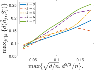
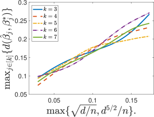
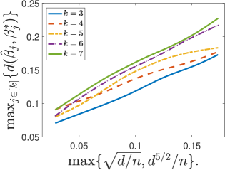
(a) $h_{1}(u)=u^{3}+10\cdot\exp(-u^{2})$	(b) $h_{2}(u)=u^{3}+5\cdot\sin(2\cdot u^{2})$,	(c) $h_{3}(u)=u^{3}+10\cdot\tanh(u^{2})$

Figure 1: Plots of the estimation error $\max_{j\in[k]}\{d(\widehat{\beta}_{j},\beta_{j}^{*})\}$ against the inverse signal strength $\max\{\sqrt{d/n},d^{3/2}/n\}$, in which $\{\widehat{\beta}_{j}\}_{j\in[k]}$ are the output of Algorithm 1 with the input moment tensor $\widehat{M}$ defined in (7). The link function is one of $h_{1}$, $h_{2}$, and $h_{3}$ in (15). The three columns correspond to $h_{1}$, $h_{2}$, and $h_{3}$, respectively. Moreover, we set $d=20$, $k\in\{3,\ldots,7\}$, and let $n$ vary. We generate each figure based on $100$ independent trials for each $(n,d,k)$.

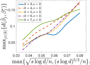
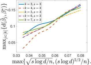
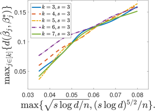
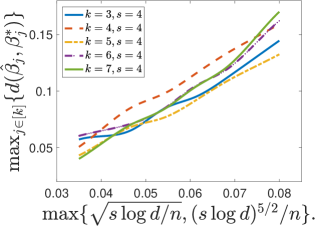
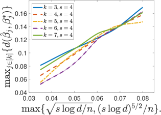
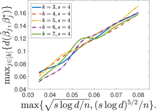
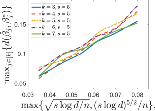
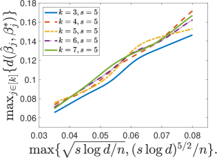
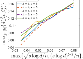
(a) $h_{1}(u)=u^{3}+10\cdot\exp(-u^{2})$	(b) $h_{2}(u)=u^{3}+5\cdot\sin(2\cdot u^{2})$,	(c) $h_{3}(u)=u^{3}+10\cdot\tanh(u^{2})$

Figure 2: Plots of the estimation error $\max_{j\in[k]}\{d(\widehat{\beta}_{j},\beta_{j}^{*})\}$ against the inverse signal strength $\max\{\sqrt{s\log d/n},(s\log d)^{5/2}/n\}$ are the output of Algorithm 1 with the input moment tensor $\widehat{M}$ defined in (7). The link function is one of $h_{1}$, $h_{2}$, and $h_{3}$ in (15). Moreover, we set $d=100$, $s\in\{3,4,5\}$, $k\in\{3,\ldots,7\}$, and let $n$ vary. We generate each figure based on $100$ independent trials for each $(n,d,s,k)$.

5 Related Work

To the best of our knowledge, there is no related work on the general DAIM considered in this work apart from linear correspondence retrieval (Andoni et al., 2017). Mixture models are a popular class of models in the literature to handle heterogeneity, with applications to regression (Chaganty and Liang, 2013; Zhong et al., 2016), classification (Jacobs et al., 1991; Sun et al., 2014; Sedghi et al., 2016) and clustering (McLachlan and Peel, 2004; Verzelen et al., 2017; Zhao et al., 2017). In terms of estimation, most of the above works focus on the parametric and/or low-dimensional setting. In comparison, handling heterogeneity in a high-dimensional and completely nonparametric setting is much more challenging. Recently, a mixture of nonparametric regression model was analyzed by Huang et al. (2013). A related technique of modal regression was also analyzed by Chen et al. (2016). Both methods are based on kernel smoothing techniques. While being completely nonparametric, they also suffer from the curse of dimensionality and are not applicable in the overcomplete setting. An interesting comprise is offered by the semiparametric single index model that we study in this work and described in detail in §2. Such a model is popular in the econometrics literature and in particular allows us to deal with the overcomplete high-dimensional setting efficiently. The recent work of Xiang and Yao (2016) also proposed a similar model in the low-dimensional setting. But they do not address the statistical and computational issues associated with estimation in such models and their estimation procedure is not applicable in the overcomplete high-dimensional setting we consider. Furthermore, recall that our estimators are based on decomposing certain higher-order moment tensors. In the recent past, several works have proposed the use of tensor decomposition techniques for estimation in several parametric latent variable models apart from the ones cited above. Apart from mixture models for prediction, such techniques have also been used for estimating means of a Gaussian mixture model  (Hsu and Kakade, 2013; Anandkumar et al., 2014a), for estimating community membership in mixed membership models (Anandkumar et al., 2013), estimating the parametric components in generalized linear model (Sedghi et al., 2016) and hidden-layer neural networks (Zhong et al., 2017; Mondelli and Montanari, 2018) and tensor sketching (Hao et al., 2018). While being related, those works essentially consider parametric latent variable models in low-dimensional settings and are not suitable to the cases with unknown links or model misspecification that we consider. Furthermore, several works have also concentrated on coming up with faster algorithm for tensor decomposition in general (see for example the recent work of  Ge and Ma (2017) and the references there in). We remark that any such algorithmic advances could be directly applicable to the model that we consider.

6 Discussion

In this work, we propose moment-based estimators for estimating the parametric components of overcomplete discordant additive index models, in both low and high-dimensional setting. Our models are motivated by sampling and heterogeneity issues common in high-dimensional big data paradigm. Our estimators are based on using tensor power method to decompose certain higher-order moment tensors. We establish statistical rate of convergence for our estimators. Numerical results are provided to corroborate the theoretical results.

We conclude the paper with a discussion of two future directions. While the main focus of the paper was on estimating the parametric components of the model in (1), one can use the estimated parametric components to obtain the nonparametric components as well as a second step, using the idea of errors in variable additive index model (Fan and Truong, 1993; Liang et al., 1999; Carroll et al., 2006). Next, in this paper we mainly considered the case of Gaussian covariates. Using the score based version of Stein’s identity (Stein et al., 2004), assuming knowledge of the density of $X$, our methods could be extended to non-Gaussian covariates. A potential issue is the score function might be heavy-tailed. Recently Yang et al. (2017) proposed a method for dealing with heavy-tailed score functions but it is not clear how to extend their approach for the overcomplete setting. Furthermore, using the zero-bias transformation version of Stein’s identity and assuming a stringent structure on the parameter vectors $\beta_{j}^{*}$, similar estimation rates with sub-Gaussian covariates could be obtained. Relaxing the Gaussian assumption, without additional assumption on either the covariates or on the parameter vectors seems to be a much harder task that we plan to address in the near future.

Appendix A Proofs of Main Results

In this section, we first provide the proofs of moment bounds, concentration bounds and net argument used to obtained the tensor concentration results. Before we proceed, we recall the definition of the $\psi_{1}$-norm and $\psi_{2}$-norm for a random variable $X$:

$$\|X\|_{\psi_{1}}=\sup_{p\geq 1}\bigl{\{}p^{-1}\cdot\bigl{(}\mathbb{E}|X|^{p}\bigr{)}^{1/p}\bigr{\}}\qquad\|X\|_{\psi_{2}}=\sup_{p\geq 1}\bigl{\{}p^{-1/2}\cdot\bigl{(}\mathbb{E}|X|^{p}\bigr{)}^{1/p}\bigr{\}}.$$ (16)

Such norms are closely associated with the notion of sub-Gaussian and sub-exponential random variables that are standard in the literature on high-dimensional statistics; we refer the reader to (Vershynin, 2010) for a detailed discussion on such random variables and associated results.

A.1 Moment Bounds

Lemma 2.

Let $\{A_{j}\}_{j\in[m]}\subseteq\mathbb{R}$ be $m$ sub-exponential random variables. Let $\Phi=\max_{j\in[m]}\|A_{j}\|_{\psi_{1}}$, then $m^{-1}\sum_{j\in[m]}A_{j}$ is a sub-exponential random variable with $\psi_{1}$-norm bounded by $\Phi$.

Proof.

For simplicity, let $B=m^{-1}\sum_{j\in[m]}A_{j}$. By the definition of $\psi_{1}$-norm, we bound $\mathbb{E}(|B|^{p})$ for any $p\geq 1$. By the triangle inequality and the AM-GM inequality, we have

$$\mathbb{E}(|B|^{p})\leq\frac{1}{m^{p}}\sum_{j_{1},j_{2},\ldots,j_{p}}\mathbb{E}\bigl{(}|A_{j_{1}}A_{j_{2}}\cdots A_{j_{p}}|\bigr{)}$$ (17)

$$\qquad\leq\frac{1}{m^{p}\cdot p}\sum_{j_{1},j_{2},\ldots,j_{p}}\bigl{[}\mathbb{E}(|A_{j_{1}}|^{p})+\ldots+\mathbb{E}(|A_{j_{p}}|^{p})\bigr{]},$$ (18)

where (17) follows from the triangle inequality, and (18) follows from the GM-AM inequality. Moreover, since $\|A_{j}\|_{\psi_{1}}\leq\Psi$ for any $j\in[m]$, we have

$$\mathbb{E}(|A_{j}|^{p})\leq(p\cdot\Phi)^{p},~{}~{}\text{for any}~{}~{}p\geq 1.$$ (19)

Thus, combining (17), (18), and (19), we obtain that $p^{-1}\cdot[\mathbb{E}(|B|^{p})]^{1/p}\leq\Phi$ for any $p\geq 1$, i.e., $\|B\|_{\psi_{1}}\leq\Phi$. Therefore, we conclude Lemma 2. ∎

A.2 Concentration Results

Since the response $Y$ in the additive index model is sub-exponential, we also need to consider concentration results involving sub-exponential random variables. For convenience of the reader, we first briefly recall the present a result on the concentration of polynomial functions of sub-Gaussian random vectors in Adamczak and Wolff (2015), which is applied in Lemma 3 below. Recall that, $X$ is sub-Gaussian if its $\psi_{2}$-norm is bounded.

Moreover, in the following, we introduce a norm for tensors, which will be used in the concentration results. Let $\ell\in\mathbb{N}_{+}$ be a positive integer. We denote by $\mathcal{P}_{\ell}$ the set of its partitions of $[\ell]$ into non-empty and non-intersecting disjoint sets. Moreover, let $A=(a_{\mathbf{i}})_{\mathbf{i}\in[n]^{\ell}}$ be a tensor of order-$\ell$, whose entries are of the form

$$a_{\mathbf{i}}=a_{i_{1},i_{2},\ldots,i_{\ell}},~{}~{}\text{where}~{}~{}{\mathbf{i}}=(i_{1},i_{2},\ldots,i_{\ell}).$$

Finally, let $\mathcal{J}=\{J_{1},\ldots,J_{k}\}\in\mathcal{P}_{\ell}$ be a fixed partition of $[\ell]$, where $J_{j}\subseteq[\ell]$ for each $j\in[k]$. Let $|\mathcal{J}|$ denote the cardinality of the $\mathcal{J}$, which is equal to $k$. We define a norm $\|\cdot\|_{\mathcal{J}}$ by

$$\|A\|_{\mathcal{J}}=\sup\Bigg{\{}\sum_{\mathbf{i}\in[n]^{\ell}}a_{\mathbf{i}}\prod_{j=1}^{k}\bm{x}^{(j)}_{{\mathbf{i}}_{J_{j}}}:\bigl{\|}\bm{x}^{(j)}\bigr{\|}_{2}\leq 1,\bm{x}^{(j)}\in\mathbb{R}^{n^{|J_{j}|}},1\leq j\leq k\Bigg{\}},$$ (20)

where we write $\mathbf{i}_{I}=(i_{k})_{k\in I}$ for any $I\subseteq[\ell]$ and the supremum is taken over all possible $k$ vectors $\{\bm{x}^{(1)},\ldots,\bm{x}^{(k)}\}$. Here each $\bm{x}^{(j)}$ in (20) is a vector of dimension $n^{|J_{j}|}$ with Euclidean norm no more than one. Suppose $J_{j}=\{t_{1},t_{2},\ldots,t_{\alpha}\}\subseteq[\ell]$, then the $\mathbf{i}_{J_{j}}$-th entry of $\bm{x}^{(j)}$ is

$$\bm{x}^{(j)}_{{\mathbf{i}}_{J_{j}}}=\bm{x}^{(j)}_{i_{t_{1}},i_{t_{2}},\ldots,i_{t_{\alpha}}}.$$

The norm defined in (20) is a generalization of some commonly seen vector and matrix norms. For example, when $\ell=1$, (20) is reduced to the Euclidean norm of vectors in $\mathbb{R}^{n}$. In addition, let $A\in\mathbb{R}^{n\times n}$ be a matrix, then $\mathcal{J}$ is a partition of $\{1,2\}$, which implies that $\mathcal{J}$ is either $\{[2]\}$ or $\{\{1\},\{2\}\}.$ By the definition in (20), we have

$$\|A\|_{\{[2]\}}=\sup\biggl{\{}\sum_{i,j\in[n]}a_{ij}x_{ij}\colon\sum_{ij\in[n]}x_{ij}^{2}\leq 1\biggr{\}}=\|A\|_{F},$$

which recovers the matrix Frobenius norm. Moreover, when $\mathcal{J}=\{\{1\},\{2\}\}$, we have

$$\|A\|_{\{1\},\{2\}}=\sup\biggl{\{}\sum_{i,j\in[n]}a_{ij}x_{i}y_{j}\colon\sum_{i\in[n]}x_{i}^{2}\leq 1,\sum_{j\in[n]}y_{j}^{2}\leq 1\biggr{\}}=\|A\|_{\operatorname{{\rm op}}},$$

which is the operator norm of $A$. Based on the norm $\|\cdot\|_{\mathcal{J}}$ defined in (20), we introduce a concentration result for polynomials of sub-Gaussian random vectors, which is a simplified version of Theorem 1.4 in Adamczak and Wolff (2015).

Theorem 11 (Theorem 1.4 Adamczak and Wolff (2015)).

Let $X=(X_{1},\ldots,X_{n})\in\mathbb{R}^{n}$ be a random vector with independent components. Moreover, we assume that such that for all $i\in[n]$, we have $\|X_{i}\|_{\psi_{2}}\leq\Upsilon$, where the $\psi_{2}$-norm is defined in (16). Then for every polynomial $F:\mathbb{R}^{n}\rightarrow\mathbb{R}$ of degree $L$, we have:

$$\mathbb{P}\bigl{(}\bigl{|}F(X)-\mathbb{E}[F(X)]\bigr{|}\geq t\bigr{)}\leq 2\exp\bigl{[}-K_{L}\cdot\eta_{F}(t)\bigr{]},$$

where the univariate function $\eta_{F}(t)$ is given by

$$\eta_{F}(t)=\min_{1\leq\ell\leq L}\min_{\mathcal{J}\in\mathcal{P}_{\ell}}\biggl{[}\frac{t}{\Upsilon^{\ell}\cdot\bigl{\|}\mathbb{E}[D^{\ell}F(X)]\bigr{\|}_{\mathcal{J}}}\biggr{]}^{2/|\mathcal{J}|}.$$ (21)

Here $\|\cdot\|_{\mathcal{J}}$ is defined in (20), $\|\cdot\|_{p}$ is the $\ell_{p}$-norm of a random variable, and $D^{\ell}F(\cdot)$ is the $\ell$-th derivative of $F$, which is takes values in the $\ell$-th order tensors.

Based on this theorem, we are ready to introduce a concentration inequality for the product of two sub-exponential random variables. This inequality might be of independent interest.

Lemma 3.

Let $\{(X_{i},Y_{i})\}_{i\in[n]}$ be $n$ independent copies of random variables $X$ and $Y$. We assume that $X$ is a sub-Gaussian random variable with $\|X\|_{\psi_{2}}\leq\Upsilon_{1}$, and $Y$ is a sub-exponential random variable with $\|Y\|_{\psi_{1}}\leq\Upsilon_{2}$ for some constants $\Upsilon_{1}$ and $\Upsilon_{2}$. Here the $\psi_{1}$- and $\psi_{2}$-norms are defined in (16). Then for any $t\geq K\cdot\max\{\Upsilon_{1}^{3},\Upsilon_{1}\}\cdot\Upsilon_{2}$, we have

$$\mathbb{P}\biggl{\{}\bigg{|}\frac{1}{n}\sum_{i=1}^{n}\big{[}X_{i}^{3}\cdot Y_{i}-\mathbb{E}(X^{3}Y)\big{]}\bigg{|}\geq t\biggr{\}}$$

$$\qquad\leq 4\exp\biggl{\{}-K_{1}\cdot\min\biggl{[}\biggl{(}\frac{t}{\sqrt{n}\Upsilon_{1}^{3}\cdot\Upsilon_{2}}\biggr{)}^{2},\biggl{(}\frac{t}{\Upsilon_{1}^{3}\cdot\Upsilon_{2}}\biggr{)}^{2/5}\biggr{]}\biggr{\}},$$ (22)

$$\mathbb{P}\biggl{\{}\bigg{|}\frac{1}{n}\sum_{i=1}^{n}\big{[}X_{i}\cdot Y_{i}-\mathbb{E}(XY)\big{]}\bigg{|}\geq t\biggr{\}}$$

$$\qquad\leq 4\exp\biggl{\{}-K_{2}\cdot\min\biggl{[}\biggl{(}\frac{t}{\sqrt{n}\Upsilon_{1}\cdot\Upsilon_{2}}\biggr{)}^{2},\biggl{(}\frac{t}{\Upsilon_{1}\cdot\Upsilon_{2}}\biggr{)}^{2/3}\biggr{]}\biggr{\}}.$$ (23)

Here $K$, $K_{1}$ and $K_{2}$ are absolute constants.

Proof.

We first establish (22). For any $i\in[n]$, we define a random variable $A_{i}^{+}$ as the positive part of $X_{i}^{3}\cdot Y_{i}$ and let $A_{i}^{-}$ be the negative part. That is, we let $A_{i}^{+}=X_{i}^{3}Y_{i}\cdot\operatorname*{\mathds{1}}\{X_{i}^{3}\cdot Y_{i}\geq 0\}$ and $A_{i}^{-}=A_{i}^{+}-X_{i}^{3}\cdot Y_{i}$. By these definitions, we have $X_{i}^{3}\cdot Y_{i}=A_{i}^{+}-A_{i}^{-}$. In the following, we establish upper bounds for

$$\mathbb{P}\biggl{(}\biggl{|}\frac{1}{n}\sum_{i=1}^{n}A_{i}^{+}-\mathbb{E}(A_{i}^{+})\bigg{|}\geq t\biggr{)}\quad\text{and}\quad\mathbb{P}\biggl{(}\biggl{|}\frac{1}{n}\sum_{i=1}^{n}A_{i}^{-}-\mathbb{E}(A_{i}^{-})\bigg{|}\geq t\biggr{)}$$ (24)

for any $t\geq K\cdot\Upsilon_{1}^{3}\cdot\Upsilon_{2}$, where $K>0$ is some absolute constant that will be specified later. Note that, by symmetry, it suffices to bound the first term in (24). Our proof utilizes the concentration inequality for polynomials of sub-Gaussian random variables, which is given in Theorem 11. To proceed, we first define $n$ random variables $Z_{i}=\eta_{i}|A_{i}^{+}|^{1/5}$ for $i\in[n]$, where $\{\eta_{i}\}_{i\in[n]}$ are $n$ independent Rademacher random variables. We show that $\{Z_{i}\}_{i\in[n]}$ are $n$ i.i.d. sub-Gaussian random variables. Notice that by definition, we have $|Z_{i}|=|A_{i}^{+}|^{1/5}\leq|X_{i}^{3}\cdot Y_{i}|^{1/5}.$ By Hölder’s inequality, for any integer $p\geq 1$, we have

$$\mathbb{E}(|Z_{i}|^{p})\leq\mathbb{E}\big{(}|X_{i}|^{3p/5}\cdot|Y_{i}|^{p/5}\big{)}\leq\bigl{[}\mathbb{E}(|X_{i}|^{3p/2})\bigr{]}^{2/5}\cdot\bigl{[}\mathbb{E}(|Y_{i}|^{p/3})\bigr{]}^{3/5}.$$ (25)

In addition, by the definition of the $\psi_{2}$-norm, we have

$$\mathbb{E}(|X_{i}|^{3p/2})\leq\bigl{(}\sqrt{3p/2}\cdot\|X\|_{\psi_{2}}\bigr{)}^{3p/2}\leq(3p/2)^{3p/4}\cdot\Upsilon_{1}^{3p/2},$$ (26)

where we use the fact that $\|X\|_{\psi_{2}}\leq\Upsilon_{1}$. Similarly, for $Y_{i}$, by the definition of the $\psi_{1}$-norm, we have

$$\mathbb{E}\bigl{(}|Y_{i}|^{p/3}\bigr{)}\leq\bigl{(}p/3\cdot\|Y_{i}\|_{\psi_{1}}\bigr{)}^{p/3}\leq(p/3)^{p/3}\cdot\Upsilon_{2}^{p/3},$$ (27)

where $\Upsilon_{2}$ is an upper bound for $\|Y\|_{\psi_{1}}$. Combining (25), (26), and (27), we obtain

$$\bigl{[}\mathbb{E}(|Z_{i}|^{p})\bigr{]}^{1/p} \leq\bigl{[}(3p/2)^{3p/10}\cdot(p/3)^{p/5}\cdot\Upsilon_{1}^{3p/5}\cdot\Upsilon_{2}^{p/5}\bigr{]}^{1/p}$$ (28)

$$\leq\sqrt{3p/2}\cdot\Upsilon_{1}^{3/5}\cdot\Upsilon_{2}^{1/5}.$$

Hence, by the definition of $\psi_{2}$-norm and (28), we have

$$\|Z_{i}\|_{\psi_{2}}=\sup_{p\geq 1}\bigl{\{}p^{-1/2}\bigl{[}\mathbb{E}(|Z_{i}|^{p})\bigr{]}^{1/p}\bigr{\}}\leq\sqrt{3/2}\cdot\Upsilon_{1}^{3/5}\cdot\Upsilon_{2}^{1/5},$$ (29)

which implies that $Z_{i}$ is a sub-Gaussian random variable with $\psi_{2}$-norm bounded by a constant depending on $\Upsilon_{1}$ and $\Upsilon_{2}$.
In the rest of the proof of (22), we establish a concentration inequality for $\{Z_{i}^{5}\}_{i\in[n]}$. To apply Theorem 11, we let $f(u)=u^{5}$ and define $F\colon\mathbb{R}^{n}\rightarrow\mathbb{R}$ by $F(z)=\sum_{i=1}^{n}f(z_{i})$. Then by definition, the high-order derivatives of $F$ are diagonal tensors whose only nonzero entries are diagonal. Specifically, for any $\ell\in[5]$ and any $i_{1},i_{2},\ldots,i_{\ell}\in[n]$, we have

$$\bigl{[}D^{\ell}F(z)\bigr{]}_{i_{1},\ldots,i_{\ell}}=\operatorname*{\mathds{1}}\{i_{1}=i_{2}=\cdots=i_{\ell}\}\cdot f^{(\ell)}(z_{i_{1}}),$$

where $z$ is an arbitrary vector in $\mathbb{R}^{n}$. To simplify the notation, for any $a_{1},\ldots,a_{n}\in\mathbb{R}$, we denote by ${\rm diag}_{\ell}\{a_{1},\ldots,a_{n}\}$ the $\ell$-th order diagonal tensor with diagonal entries $a_{1},a_{2},\ldots,a_{n}$. Using this notation, for any $\ell\in[5]$, we can write

$$D^{\ell}F(z)={\rm diag}_{\ell}\bigl{[}f^{(\ell)}(z_{1}),\ldots,f^{(\ell)}(z_{n})\bigr{]}.$$ (30)

Moreover, for diagonal tensors, the norm $\|\cdot\|_{\mathcal{J}}$ defined in (20) have simple forms. For any $a\in\mathbb{R}^{n}$ and any integer $\ell\geq 1$, we have

$$\|{\rm diag}_{\ell}\{a_{1},\ldots,a_{n}\}\|_{\mathcal{J}}=\operatorname*{\mathds{1}}\{|\mathcal{J}|=1\}\cdot\|a\|_{2}+\operatorname*{\mathds{1}}\{|\mathcal{J}|\geq 2\}\cdot\|a\|_{\max}.$$ (31)

In addition, note that $|f^{(\ell)}(u)|\leq 5!\cdot|u|^{5-\ell}$ for any $u\in\mathbb{R}$. For i.i.d. random variables $\{Z_{i}\}_{i\in[n]}$, we define $Z=(Z_{1},\ldots,Z_{n})^{\top}$. Combining (30) and (43), we obtain

$$\bigl{\|}\mathbb{E}[D^{\ell}F(Z)]\bigr{\|}_{\mathcal{J}} =\operatorname*{\mathds{1}}\{|\mathcal{J}|=1\}\cdot\sqrt{n}\cdot\bigl{|}\mathbb{E}[f^{(\ell)}(Z_{1})]\bigr{|}+\operatorname*{\mathds{1}}\{|\mathcal{J}|\geq 2\}\bigl{|}\mathbb{E}[f^{(\ell)}(Z_{1})]\bigr{|}.$$ (32)

Now we are ready to apply Theorem 11. The function $\eta_{F}(t)$ defined in (21) now becomes

$$\eta_{F}(t)=\min_{\ell\in[5]}\min_{\mathcal{J}\in\mathcal{P}_{\ell}}\Bigl{\{}t\cdot\|Z_{1}\|_{\psi_{2}}^{-\ell}\cdot\bigl{\|}\mathbb{E}[D^{\ell}F(Z)]\bigr{\|}_{\mathcal{J}}^{-1}\Bigr{\}}^{2/|\mathcal{J}|}.$$ (33)

Note that the tail probability in Theorem 11 is equal to $\exp[-K\cdot\eta_{F}(t)]$, where $K$ is an absolute constant. To upper bound this term, in the sequel, we establish an lower bound for $\eta_{F}(t)$. We first establish an upper bound for $\bigl{\|}\mathbb{E}[D^{\ell}F(Z)]\bigr{\|}_{\mathcal{J}}$. Since $f(u)=u^{5}$, we have $|f^{\ell}(u)|\leq 5!\cdot|u|^{5-\ell}$. Thus, by (32) we have

$$\bigl{\|}\mathbb{E}[D^{\ell}F(Z)]\bigr{\|}_{\mathcal{J}}\leq 5!\cdot\bigl{(}\operatorname*{\mathds{1}}\{|\mathcal{J}|=1\}\cdot\sqrt{n}+\operatorname*{\mathds{1}}\{|\mathcal{J}|\geq 2\}\bigr{)}\cdot\mathbb{E}\bigl{(}|Z_{1}|^{5-\ell}\bigr{)}.$$

Note that $Z_{1}$ is a sub-Gaussian random variable. By the definition of $\psi_{2}$-norm in (16), we have $\mathbb{E}(|Z_{1}|^{k})\leq(\sqrt{k})^{k}\cdot\|Z_{1}\|^{k}_{\psi_{2}}$ for any $k\geq 0$, where we follow the convention by letting $0^{0}=1$. Therefore, by (32) we have

$$\bigl{\|}\mathbb{E}[D^{\ell}F(Z)]\bigr{\|}_{\mathcal{J}}$$

$$\quad\leq 25\cdot\big{(}\sqrt{5-\ell}\big{)}^{5-\ell}\cdot\bigl{(}\operatorname*{\mathds{1}}\{|\mathcal{J}|=1\}\cdot\sqrt{n}+\operatorname*{\mathds{1}}\{|\mathcal{J}|\geq 2\}\bigr{)}\cdot\|Z_{1}\|^{5-\ell}_{\psi_{2}},$$ (34)

for any $\ell\in[5]$. We denote $C_{\ell}=25\cdot(5-\ell)^{(5-\ell)/2}$ to simplify the notation, which is an absolute constant. Now we combine (33) and (A.2) to obtain

$$\|Z_{1}\|_{\psi_{2}}^{\ell}\cdot\bigl{\|}\mathbb{E}[D^{\ell}F(Z)]\bigr{\|}_{\mathcal{J}}\leq C_{\ell}\cdot\bigl{(}\operatorname*{\mathds{1}}\{|\mathcal{J}|=1\}\cdot\sqrt{n}+\operatorname*{\mathds{1}}\{|\mathcal{J}|\geq 2\}\bigr{)}\cdot\|Z_{1}\|^{5}_{\psi_{2}}.$$

Plugging this inequality in (33), we have

$$\eta_{F}(t)\geq\min_{\ell\in[5]}\Bigl{\{}\min\Bigl{[}\bigl{(}t/\sqrt{n}\cdot C_{\ell}^{-1}\|Z_{1}\|_{\psi_{2}}^{-5}\bigr{)}^{2},\min_{2\leq|\mathcal{J}|\leq\ell}\bigl{(}t\cdot C_{\ell}^{-1}\|Z_{1}\|_{\psi_{2}}^{-5}\bigr{)}^{2/|\mathcal{J}|}\Bigr{]}\Bigr{\}}.$$

When $t>C_{\ell}\cdot\|Z_{1}\|_{\psi_{2}}^{5}$ for any $\ell\in\{2,\ldots,5\}$, we simplify the above inequality by

$$\eta_{F}(t) \geq\min\Bigl{\{}\min_{\ell\in[5]}\Bigl{[}\bigl{(}t/\sqrt{n}\cdot C_{\ell}^{-1}\|Z_{1}\|_{\psi_{2}}^{-5}\bigr{)}^{2}\Bigr{]},\min_{2\leq\ell\leq 5}\Bigl{[}\bigl{(}t\cdot C_{\ell}^{-1}\|Z_{1}\|_{\psi_{2}}^{-5}\bigr{)}^{2/\ell}\Bigr{]}\Bigr{\}}$$

$$=\min\Bigl{\{}\bigl{(}t/\sqrt{n}\cdot\widetilde{C}_{0}^{-1}\|Z_{1}\|_{\psi_{2}}^{-5}\bigr{)}^{2},\min_{2\leq\ell\leq 5}\Bigl{[}\bigl{(}t\cdot C_{\ell}^{-1}\|Z_{1}\|_{\psi_{2}}^{-5}\bigr{)}^{2/\ell}\Bigr{]}\Bigr{\}},$$ (35)

where we define $\widetilde{C}_{0}=\max_{\ell\in[5]}C_{\ell}$. Note that the $\psi_{2}$-norm of $Z_{1}$ is bounded in (29), which implies

$$C_{\ell}\cdot\|Z_{1}\|_{\psi_{2}}^{5}\leq K\cdot\Upsilon_{1}^{3}\cdot\Upsilon_{2}$$ (36)

for all $\ell\in[5]$, where $K$ is some absolute constant. We denote the term on the right-hand side of (36) by $K_{\Upsilon}$ for simplicity.

Thus, combining (A.2) and (36), we have

$$\eta_{F}(t)\geq\min\bigl{\{}\bigl{[}t/(\sqrt{n}\cdot K_{\Upsilon})\bigr{]}^{2},\min_{2\leq\ell\leq 5}(t/K_{\Upsilon})^{2/\ell}\bigr{\}}.$$

When $t\geq K_{\Upsilon}$, we have

$$\eta_{F}(t)\geq\min\bigl{\{}\bigl{[}t/(\sqrt{n}\cdot K_{\Upsilon})\bigr{]}^{2},(t/K_{\Upsilon})^{2/5}\bigr{\}}.$$ (37)

Plugging (37) in Theorem 11, since $|Z_{i}|^{5}=|A_{i}^{+}|=A_{i}^{+}$, when $t\geq 2K_{\Upsilon}$, we obtain

$$\mathbb{P}\biggl{[}\biggl{|}\sum_{i=1}^{n}A_{i}^{+}-\mathbb{E}(A_{i}^{+})\biggr{|}\geq t/2\biggr{]} \leq 2\exp\bigl{[}-C\cdot\eta_{F}(t/2)\bigr{]}$$

$$\leq 2\exp\Bigl{(}-C\min\bigl{\{}\bigl{[}t/(2\sqrt{n}\cdot K_{\Upsilon})\bigr{]}^{2},[t/(2K_{\Upsilon})]^{2/5}\bigr{\}}\Bigr{)},$$ (38)

where $C$ is an absolute constant that does not rely on $\Upsilon_{1}$ and $\Upsilon_{2}$. Similarly, for $A_{i}^{-}$, using the same analysis, we obtain that

$$\mathbb{P}\biggl{[}\biggl{|}\sum_{i=1}^{n}A_{i}^{-}-\mathbb{E}(A_{i}^{-})\biggr{|}\geq t/2\biggr{]}$$

$$\quad\leq 2\exp\Bigl{(}-C\min\bigl{\{}\bigl{[}t/(2\sqrt{n}\cdot K_{\Upsilon})\bigr{]}^{2},[t/(2K_{\Upsilon})]^{2/5}\bigr{\}}\Bigr{)}.$$ (39)

Note that $|a-b|\geq t$ implies that $|a|\geq t/2$ or $|b|\geq t/2$ for any $a,b\in\mathbb{R}$ and $t>0$. Combining (A.2) and (A.2), we finally obtain

$$\mathbb{P}\biggl{[}\biggl{|}\sum_{i=1}^{n}X_{i}^{3}\cdot Y-\mathbb{E}(X^{3}\cdot Y)\biggr{|}\geq t\biggr{]}$$

$$\quad\leq\mathbb{P}\biggl{[}\biggl{|}\sum_{i=1}^{n}A_{i}^{+}-\mathbb{E}(A_{i}^{+})\biggr{|}\geq t/2\biggr{]}+\mathbb{P}\biggl{[}\biggl{|}\sum_{i=1}^{n}A_{i}^{-}-\mathbb{E}(A_{i}^{-})\biggr{|}\geq t/2\biggr{]}$$

$$\quad\leq 4\exp\biggl{\{}-K_{1}\cdot\min\biggl{[}\biggl{(}\frac{t}{\sqrt{n}\Upsilon_{1}^{3}\cdot\Upsilon_{2}}\biggr{)}^{2},\biggl{(}\frac{t}{\Upsilon_{1}^{3}\cdot\Upsilon_{2}}\biggr{)}^{2/5}\biggr{]}\biggr{\}},$$ (40)

where $K_{1}$ is an absolute constant. Note that, by (36), here we require $t\geq K\cdot\Upsilon_{1}^{3}\cdot\Upsilon_{2}$ for some constant $K$. Thus, we establish (22).

To conclude the proof of this lemma, it remains to show (23). The proof is similar to the derivations above. Now, for any $i\in[n]$, we define $B_{i}^{+}$ and $B_{i}^{-}$ as the positive and negative parts of $X_{i}\cdot Y_{i}$, respectively. Then we have $X_{i}\cdot Y_{i}=B_{i}^{+}-B_{i}^{-}$ by definition.

We first establish a concentration inequality for $\{B_{i}^{+}\}_{i\in[n]}$. To utilize Theorem 11. To proceed, we first define $Z_{i}=\eta_{i}|B_{i}^{+}|^{1/3}$ for $i\in[n]$, where $\{\eta_{i}\}_{i\in[n]}$ are $n$ independent Rademacher random variables. Then we show that $\{Z_{i}\}_{i\in[n]}$ are $n$ i.i.d. sub-Gaussian random variables. For any integer $p\geq 1$, Hölder’s inequality implies that

$$\mathbb{E}(|Z_{i}|^{p})\leq\mathbb{E}\big{(}|X_{i}|^{p/3}\cdot|Y_{i}|^{p/3}\big{)}\leq\bigl{[}\mathbb{E}(|X_{i}|^{p/2})\bigr{]}^{2/3}\cdot\bigl{[}\mathbb{E}(|Y_{i}|^{p})\bigr{]}^{1/3}.$$ (41)

Moreover, since $\|X\|_{\psi_{2}}\leq\Upsilon_{1}$ and $\|Y\|_{\psi_{1}}\leq\Upsilon_{2}$, by the definition of the $\psi_{2}$- and $\psi_{1}$-norms, we have

$$\mathbb{E}(|X_{i}|^{p/2}) \leq\bigl{(}\sqrt{p/2}\cdot\|X\|_{\psi_{2}}\bigr{)}^{p/2}\leq(p/2)^{p/4}\cdot\Upsilon_{1}^{p/2},$$ (42)

$$\mathbb{E}(|Y_{i}|^{p}) \leq\bigl{(}p\cdot\|Y_{i}\|_{\psi_{1}}\bigr{)}^{p}\leq p^{p}\cdot\Upsilon_{2}^{p}.$$

Thus, combining (41) and (42), we obtain

$$\bigl{[}\mathbb{E}(|Z_{i}|^{p})\bigr{]}^{1/p}\leq\bigl{[}(p/2)^{p/6}\cdot p^{p/3}\cdot\Upsilon_{1}^{2p/3}\cdot\Upsilon_{2}^{p/3}\bigr{]}^{1/p}\leq\sqrt{p}\cdot\Upsilon_{1}^{1/3}\cdot\Upsilon_{2}^{1/3},$$

which implies that $\|Z_{i}\|_{\psi_{2}}\leq\Upsilon_{1}^{1/3}\cdot\Upsilon_{2}^{1/3}.$ Thus, $Z_{i}$ is a sub-Gaussian random variable with $\psi_{2}$-norm bounded by $\Upsilon_{1}^{1/3}\cdot\Upsilon_{2}^{1/3}$.

To prove (23), we establish a concentration inequality for $\{Z_{i}^{3}\}_{i\in[n]}$. Similar to the pervious case, we let $f(u)=u^{3}$ and define $F\colon\mathbb{R}^{n}\rightarrow\mathbb{R}$ by $F(z)=\sum_{i=1}^{n}f(z_{i})$. By this construction, for any $\ell\in\{1,2,3\}$, the $\ell$-th order derivative of $F$ is given by

$$D^{\ell}F(z)={\rm diag}_{\ell}\bigl{[}f^{(\ell)}(z_{1}),\ldots,f^{(\ell)}(z_{n})\bigr{]}.$$ (43)

Note that here $D^{\ell}F(z)$ has the same form as (30). Similar to (A.2), we have

$$\|Z_{1}\|^{\ell}_{\psi_{2}}\cdot\bigl{\|}\mathbb{E}[D^{\ell}F(Z)]\bigr{\|}_{\mathcal{J}}$$

$$\quad\leq 3!\cdot\big{(}\sqrt{3-\ell}\big{)}^{3-\ell}\cdot\bigl{(}\operatorname*{\mathds{1}}\{|\mathcal{J}|=1\}\cdot\sqrt{n}+\operatorname*{\mathds{1}}\{|\mathcal{J}|\geq 2\}\bigr{)}\cdot\|Z_{1}\|^{3}_{\psi_{2}}$$

$$\quad\leq K\cdot\bigl{(}\operatorname*{\mathds{1}}\{|\mathcal{J}|=1\}\cdot\sqrt{n}+\operatorname*{\mathds{1}}\{|\mathcal{J}|\geq 2\}\bigr{)}\cdot\Upsilon_{1}\cdot\Upsilon_{2},$$ (44)

where $K$ is a constant that does not depend on $\Upsilon_{1}$ and $\Upsilon_{2}$. Moreover, by (A.2), for any $t$ satisfying $t\geq K\cdot\Upsilon_{1}\cdot\Upsilon_{2}$, the function $\eta_{F}(t)$ defined in (21) can be lower bounded by

$$\eta_{F}(t) =\min_{\ell\in[3]}\min_{\mathcal{J}\in\mathcal{P}_{\ell}}\Bigl{\{}t\cdot\|Z_{1}\|_{\psi_{2}}^{-\ell}\cdot\bigl{\|}\mathbb{E}[D^{\ell}F(Z)]\bigr{\|}_{\mathcal{J}}^{-1}\Bigr{\}}^{2/|\mathcal{J}|}$$

$$s\geq\min\bigl{\{}\bigl{[}t\big{/}(\sqrt{n}\cdot K\Upsilon_{1}\Upsilon_{2})\bigr{]}^{2},\bigl{[}t\big{/}(K\Upsilon_{1}\Upsilon_{2})\bigr{]}^{2/3}\bigr{\}}.$$ (45)

Note that $|Z_{i}|^{3}=|B_{i}^{+}|=B_{i}^{+}$. Plugging (A.2) in Theorem 11, for any $t$ satisfying $t\geq 2K\cdot\Upsilon_{1}\cdot\Upsilon_{2}$, we have

$$\mathbb{P}\biggl{[}\biggl{|}\sum_{i=1}^{n}B_{i}^{+}-\mathbb{E}(B_{i}^{+})\biggr{|}\geq t/2\biggr{]}\leq 2\exp\bigl{[}-C\cdot\eta_{F}(t/2)\bigr{]}$$

$$\quad\leq 2\exp\Bigl{(}-C\min\bigl{\{}\bigl{[}t/(2\sqrt{n}\cdot K\Upsilon_{1}\Upsilon_{2})\bigr{]}^{2},[t/(2K\Upsilon_{1}\Upsilon_{2})]^{2/3}\bigr{\}}\Bigr{)},$$ (46)

where $C$ is an absolute constant that is does not reply on $\Upsilon_{1}$ and $\Upsilon_{2}$. Similarly, using the same analysis, we obtain a similar concentration inequality for $\{B_{i}^{-}\}_{i\in[n]}$:

$$\mathbb{P}\biggl{[}\biggl{|}\sum_{i=1}^{n}B_{i}^{-}-\mathbb{E}(B_{i}^{-})\biggr{|}\geq t/2\biggr{]}$$

$$\quad\leq 2\exp\Bigl{(}-C\min\bigl{\{}\bigl{[}t/(2\sqrt{n}\cdot K\Upsilon_{1}\Upsilon_{2})\bigr{]}^{2},[t/(2K\Upsilon_{1}\Upsilon_{2})]^{2/3}\bigr{\}}\Bigr{)}.$$ (47)

Therefore, combining (A.2) and (A.2), we finally obtain that

$$\mathbb{P}\biggl{[}\biggl{|}\sum_{i=1}^{n}X_{i}\cdot Y-\mathbb{E}(X\cdot Y)\biggr{|}\geq t\biggr{]}s$$

$$\quad\leq 4\exp\Bigl{(}-K_{2}\cdot\min\bigl{\{}\bigl{[}t/(2\sqrt{n}\cdot\Upsilon_{1}\Upsilon_{2})\bigr{]}^{2},[t/(2\Upsilon_{1}\Upsilon_{2})]^{2/3}\bigr{\}}\Bigr{)}$$ (48)

where $K_{2}$ is an absolute constant. Note that here we require $t\geq K\cdot\Upsilon_{1}\Upsilon_{2}$ for some absolute constant $K>0$. Therefore, combining (A.2) and (A.2), we conclude the proof of Lemma 3. ∎

A.3 Net Argument for Tensor Operator Norm

In this section, we prove the $\epsilon$-net argument for tensor operator norm. The $\epsilon$-net argument is a standard technique for bounding the operator norm of matrices, whereas its construction is relatively more involved in the tensor case.

In the sequel, for generality, we focus on $\ell$-th order tensors in $\mathbb{R}^{d}$. For any $\ell$-th order tensor $A\in\mathbb{R}^{d\otimes\ell}$, the operator norm of $A$ is given by

$$\|A\|_{\operatorname{{\rm op}}}=\sup\bigl{\{}\bigl{|}A(u^{(1)},\ldots,u^{(\ell)})\bigr{|}\colon u^{(1)},u^{(2)},\ldots,u^{(\ell)}\in{\mathcal{S}}^{d-1}\bigr{\}},$$ (49)

where ${\mathcal{S}}^{d-1}$ is the unit sphere in $\mathbb{R}^{d}$. In addition, for any $r\in[d]$, we define the $r$-sparse subset of ${\mathcal{S}}^{d-1}$ as

$${\mathcal{S}}^{d-1}(r)=\bigl{\{}u\in\mathbb{R}^{d}\colon\|u\|_{2}=1,\|u\|_{0}\leq r\bigr{\}}.$$ (50)

Then the sparse tensor norm of $A$ is defined by

$$\|A\|_{\operatorname{{\rm op}},r}=\sup\bigl{\{}\bigl{|}A(u^{(1)},\ldots,u^{(\ell)})\bigr{|}\colon u^{(1)},u^{(2)},\ldots,u^{(\ell)}\in{\mathcal{S}}^{d-1}(r)\bigr{\}}.$$ (51)

Moreover, for any set $\mathcal{E}\subseteq\mathbb{R}^{d}$, we say $\mathcal{N}$ is an $\epsilon$-net for $\mathcal{E}$, if for any $u\in\mathcal{E}$, there exists $v\in\mathcal{N}$ such that $\|u-v\|_{2}\leq\epsilon$. Then we are ready to present the $\epsilon$-argument for $\ell$-th order tensors, which is given in the following lemma.

Lemma 4 ($\epsilon$-net argument for tensors).

For any $\epsilon\in(0,1/\ell)$, let $\mathcal{N}_{{\mathcal{S}}}(\epsilon)$ and $\mathcal{N}_{{\mathcal{S}}}(\epsilon,r)$ be the $\epsilon$-nets of ${\mathcal{S}}^{d-1}$ and ${\mathcal{S}}^{d-1}(r)$, respectively. Then for any $\ell$-th order tensor $A\in\mathbb{R}^{d\otimes\ell}$, we have

$$\|A\|_{\operatorname{{\rm op}}} \leq(1-\ell\cdot\epsilon)^{-1}\cdot\sup\bigl{\{}\bigl{|}A(u^{(1)},\ldots,u^{(\ell)})\bigr{|}\colon\{u^{(j)}\}_{j\in[\ell]}\subseteq\mathcal{N}_{{\mathcal{S}}}(\epsilon)\bigr{\}},$$ (52)

$$\|A\|_{\operatorname{{\rm op}},r} \leq(1-\ell\cdot\epsilon)^{-1}\cdot\sup\bigl{\{}\bigl{|}A(u^{(1)},\ldots,u^{(\ell)})\bigr{|}\colon\{u^{(j)}\}_{j\in[\ell]}\subseteq\mathcal{N}_{{\mathcal{S}}}(\epsilon,r)\bigr{\}}.$$ (53)

Moreover, when $A$ is a symmetric tensor, we further have

$$\|A\|_{\operatorname{{\rm op}}} \leq(1-\ell\cdot\epsilon)^{-1}\cdot\sup_{u\in\mathcal{N}_{{\mathcal{S}}}(\epsilon)}\bigl{|}A(u,u,\ldots,u)\bigr{|},$$ (54)

$$\|A\|_{\operatorname{{\rm op}},r} \leq(1-\ell\cdot\epsilon)^{-1}\cdot\sup_{u\in\mathcal{N}_{{\mathcal{S}}}(\epsilon,r)}\bigl{|}A(u,u,\ldots,u)\bigr{|}.$$ (55)

Note that our Lemma 4 covers the $\epsilon$-argument for matrices by setting $\ell=2$. In this case, we have

$$\|A\|_{\operatorname{{\rm op}}}=\sup_{x,y\in{\mathcal{S}}^{d}}x^{\top}Ay\leq(1-2\epsilon)^{-1}\sup_{x,y\in\mathcal{N}_{{\mathcal{S}}}(\epsilon)}x^{\top}Ay,$$

which is the Lemma 5.4 in Vershynin (2010).

Proof of Lemma 4.

In the following, we first prove the results for $\|\cdot\|_{\operatorname{{\rm op}}}$. Let $A\in\mathbb{R}^{d\otimes\ell}$ be a $\ell$-th order tensor. By the definition of the tensor spectral norm, there exist $u^{(1)},\ldots,u^{(\ell)}\in{\mathcal{S}}^{d-1}$ such that $\|A\|_{\operatorname{{\rm op}}}=A(u^{(1)},\ldots,u^{(\ell)}).$ Moreover, for any $j\in[\ell]$ , there exists $v^{(j)}\in\mathcal{N}_{{\mathcal{S}}}(\epsilon)$ such that $\|u^{(j)}-v^{(j)}\|_{2}\leq\epsilon$. In the following, we prove tbound the difference between $A(u^{(1)},\ldots,u^{(\ell)})$ and $A(v^{(1)},\ldots,v^{(\ell)})$. To simplify the notation, we define $\delta^{(j)}=u^{(j)}-v^{(j)}$ by and let $\bar{\delta}^{(j)}=\delta^{(j)}/\|\delta^{(j)}\|_{2}$ for all $j\in[\ell]$. By triangle inequality, we have

$$\bigl{|}A(u^{(1)},\ldots,u^{(\ell)})-A(v^{(1)},\ldots,v^{(\ell)})\bigr{|}$$

$$\quad\leq\bigl{|}A(u^{(1)},\ldots,u^{(\ell)})-A(u^{(1)},\ldots,u^{(\ell-1)},v^{(\ell)})\bigr{|}$$

$$\quad\quad\quad+\bigl{|}A(u^{(1)},\ldots,u^{(\ell-1)},v^{(\ell)})-A(v^{(1)},\ldots,v^{(\ell)})\bigr{|}.$$ (56)

For the first term on the right-hand side of (A.3), we have

$$\bigl{|}A(u^{(1)},\ldots,u^{(\ell)})-A(u^{(1)},\ldots,u^{(\ell-1)},v^{(\ell)})\bigr{|}=\bigl{|}A(u^{(1)},\ldots,u^{(\ell-1)},\delta^{(\ell)})\bigr{|}$$

$$\quad=\bigl{|}A(u^{(1)},\ldots,u^{(\ell-1)},\bar{\delta}^{(\ell)})\bigr{|}\cdot\|\delta^{(\ell)}\|_{2}\leq\|\delta^{(\ell)}\|_{2}\cdot\|A\|_{\operatorname{{\rm op}}},$$

where the last inequality follows from the the definitions of $\|A\|_{\operatorname{{\rm op}}}$. Similarly, for the second term, we have

$$\bigl{|}A(u^{(1)},\ldots,u^{(\ell-1)},v^{(\ell)})-A(v^{(1)},\ldots,v^{(\ell)})\bigr{|}$$

$$\quad\leq\bigl{|}A(u^{(1)},\ldots,u^{(\ell-1)},v^{(\ell)})-A(u^{(1)},\ldots,u^{(\ell-2)},v^{(\ell-1)},v^{(\ell)})\bigr{|}$$

$$\quad\quad+\bigl{|}A(u^{(1)},\ldots,u^{(\ell-2)},v^{(\ell-1)},v^{(\ell)})-A(v^{(1)},\ldots,v^{(\ell)})\bigr{|}$$

$$\quad\leq\|\delta^{(\ell-1)}\|_{2}\cdot\|A\|_{\operatorname{{\rm op}}}+\bigl{|}A(u^{(1)},\ldots,u^{(\ell-2)},v^{(\ell-1)},v^{(\ell)})-A(v^{(1)},\ldots,v^{(\ell)})\bigr{|}.$$

Continuing the same argument, we finally obtain that

$$\bigl{|}A(u^{(1)},\ldots,u^{(\ell)})-A(v^{(1)},\ldots,v^{(\ell)})\bigr{|}$$

$$\quad\leq\bigl{(}\|\delta^{(1)}\|_{2}+\ldots+\|\delta^{(\ell)}\|_{2}\bigr{)}\cdot\|A\|_{\operatorname{{\rm op}}}\leq\ell\cdot\epsilon\cdot\|A\|_{\operatorname{{\rm op}}},$$ (57)

where the last inequality follows from the definition of $\mathcal{N}_{{\mathcal{S}}}(\epsilon)$. Thus, by triangle inequality, we have

$$|A(v^{(1)},\ldots,v^{(\ell)})| \geq\bigl{|}A(u^{(1)},\ldots,u^{(\ell)})\bigr{|}-\bigl{|}A(u^{(1)},\ldots,u^{(\ell)})-A(v^{(1)},\ldots,v^{(\ell)})\bigr{|}$$

$$\geq(1-\ell\cdot\epsilon)\cdot\|A\|_{\operatorname{{\rm op}}},$$

which proves (52). Moreover, when $A$ is a symmetric tensor, we could choose $u^{(1)}=u^{(2)}=\ldots=u^{(\ell)}=u\in{\mathcal{S}}^{d-1}$ and $v^{(1)}=v^{(2)}=\ldots=v^{(\ell)}=v\in\mathcal{N}_{{\mathcal{S}}}(\epsilon)$ such that $\|A\|_{\operatorname{{\rm op}}}=A(u,\ldots,u)$ and $\|u-v\|_{2}\leq\epsilon$. Then by (A.3) we have

$$|A(v,\ldots,v)| \geq\bigl{|}A(u,\ldots,u)\bigr{|}-\bigl{|}A(u,\ldots,u)-A(v,\ldots,v)\bigr{|}$$

$$\geq\bigl{(}1-\ell\cdot\|u-v\|_{2}\bigr{)}\cdot\|A\|_{\operatorname{{\rm op}}}\geq(1-\ell\cdot\epsilon)\cdot\|A\|_{\operatorname{{\rm op}}},$$

which concludes (54). Following the same argument with ${\mathcal{S}}^{d-1}$ and $\mathcal{N}_{{\mathcal{S}}}(\epsilon)$ replaced by ${\mathcal{S}}^{d-1}(r)$ and $\mathcal{N}_{{\mathcal{S}}}(\epsilon,r)$, respectively, we also have (53) and (55). Thus, we conclude the proof. ∎

A.4 Proof of Theorem 4

In this section, we present the proof of Theorem 4. Since the results for $\widehat{M}_{1}$ and $\widehat{M}_{2}$ are established using similar techniques, in the following, we first present a detailed proof of the bound on $\|\widehat{M}_{2}-\mathbb{E}[h_{2}(\mathcal{Z})\cdot S_{3}(X)]\|_{\operatorname{{\rm op}}}$, then prove the other part by showing the differences.

Upper bound for $\|\widehat{M}_{2}-\mathbb{E}[h_{2}(\mathcal{Z})\cdot S_{3}(X)]\|_{\operatorname{{\rm op}}}$. First note that by the definition of third order score function $S_{3}$ in (5), we have $\widehat{M}_{2}=\widehat{T}_{1}+\widehat{T}_{2},$ where $\widehat{M}_{2}$ is given in (8), and we define $\widehat{T}_{1}$ and $\widehat{T}_{2}$ respectively by

$$\widehat{T}_{1} =\frac{1}{n}\sum_{i=1}^{n}Y^{(i)}\cdot X^{(i)}\otimes X^{(i)}\otimes X^{(i)},$$ (58)

$$\widehat{T}_{2} =\frac{1}{n}\sum_{i=1}^{n}\sum_{j=1}^{d}Y^{(i)}\cdot\bigl{(}X^{(i)}\otimes e_{j}\otimes e_{j}+e_{j}\otimes X^{(i)}\otimes e_{j}+e_{j}\otimes e_{j}\otimes X^{(i)}\bigr{)},$$ (59)

where $Y^{(i)}=h_{2}(\mathcal{Z}^{(i)})$ is the response of of the mixture of SIMs. Note that we have

$$\mathbb{E}(\widehat{M}_{2})=\mathbb{E}[h_{2}(\mathcal{Z})\cdot S_{3}(X)]=\sum_{j=1}^{k}\gamma_{j}^{*}\cdot\theta_{j}^{*\otimes 3},$$

where the second equality follows from Lemma 1. By the triangle inequality, we have

$$\bigl{\|}\widehat{M}_{2}-\mathbb{E}(\widehat{M}_{2})\bigr{\|}_{\operatorname{{\rm op}}}\leq\bigl{\|}\widehat{T}_{1}-\mathbb{E}(\widehat{T}_{1})\bigr{\|}_{\operatorname{{\rm op}}}+\bigl{\|}\widehat{T}_{2}-\mathbb{E}(\widehat{T}_{2})\bigr{\|}_{\operatorname{{\rm op}}}.$$ (60)

In the sequel, we upper bound the two terms on the right-hand of (60) separately.

First, since $\widehat{T}_{1}$ and $\widehat{T}_{2}$ defined in (58) and (59) are symmetric tensors, the definition of tensor operator norm in (49) yields that

$$\bigl{\|}\widehat{T}_{1}-\mathbb{E}(\widehat{T}_{1})\bigr{\|}_{\operatorname{{\rm op}}}=\sup_{u\in{\mathcal{S}}^{d-1}}\Bigl{\{}\Bigl{|}\widehat{T}_{1}(u,u,u)-\mathbb{E}\bigl{[}\widehat{T}_{1}(u,u,u)\bigr{]}\Bigr{|}\Bigr{\}},$$ (61)

where ${\mathcal{S}}^{d-1}=\{u\in\mathbb{R}^{d}\colon\|u\|_{2}=1\}$ is the unit sphere in $\mathbb{R}^{d}$. Similar to showing the concentration of random matrices, our derivation consists of two steps. In the first step, we firstly apply the $\epsilon$-net argument for tensor operator norm. Then we bound the concentration of $|\widehat{T}_{1}(u,u,u)-\mathbb{E}[\widehat{T}_{1}(u,u,u)]|$ for any fixed $u\in{\mathcal{S}}^{d-1}$ and apply a union bound over the $\epsilon$-net.

To begin with, let $N_{{\mathcal{S}}}(\epsilon)$ be the $\epsilon$-net of the unit sphere ${\mathcal{S}}^{d-1}$ for any $\epsilon\in(0,1)$. We now appeal to Lemma 4, which shows that taking the supremum in (61) over $N_{{\mathcal{S}}}(1/6)$ instead of ${\mathcal{S}}^{d-1}$ only incurs a small error. Specifically, we apply Lemma 4 with $\ell=3$, and $\epsilon=1/6$ to $\widehat{T}_{1}$ to obtain

$$\bigl{\|}\widehat{T}_{1}-\mathbb{E}(\widehat{T}_{1})\bigr{\|}_{\operatorname{{\rm op}}}\leq 2\sup_{u\in\mathcal{N}_{{\mathcal{S}}}(1/6)}\Bigl{\{}\Bigl{|}\widehat{T}_{1}(u,u,u)-\mathbb{E}\bigl{[}\widehat{T}_{1}(u,u,u)\bigr{]}\Bigr{|}\Bigr{\}}.$$ (62)

In the next step, we derive a concentration inequality for $\widehat{T}_{1}(u,u,u)$ with fixed $u\in{\mathcal{S}}^{d-1}$, and apply a union bound of $\mathcal{N}_{{\mathcal{S}}}(1/6)$ to conclude the proof.

By the definition of $\widehat{T}_{1}$ in (58), we have we have

$$\widehat{T}_{1}(u,u,u)=\frac{1}{n}\sum_{i=1}^{n}Y^{(i)}\cdot(X^{(i)\top}u)^{3}.$$

By Assumption 1, $\{Y^{(i)}\}_{i\in[n]}$ are i.i.d. sub-exponential random variables with $\psi_{1}$-norm bounded by $\Psi$. Moreover, since $\{X^{(i)}\}_{i\in[n]}$ are i.i.d. $N(0,I_{d})$ random vectors, $X^{(i)\top}u$ are independent standard Gaussian random variables for each $u\in{\mathcal{S}}^{d-1}$. Thus $\|X^{(i)\top}u\|_{\psi_{2}}\leq\Upsilon_{0}$ where $\Upsilon_{0}$ is a constant. To bound $|\widehat{T}_{1}(u,u,u)-\mathbb{E}[\widehat{T}_{1}(u,u,u)]|$, we apply (22) in Lemma 3 to obtain that

$$\mathbb{P}\Bigl{\{}\Bigl{|}\widehat{T}_{1}(u,u,u)-\mathbb{E}\bigl{[}\widehat{T}_{1}(u,u,u)\bigr{]}\Bigr{|}\geq t/n\Bigr{\}}$$

$$\quad\leq 4\exp\Bigl{(}-K_{1}\cdot\min\big{\{}[t/(\sqrt{n}\Upsilon_{0}^{3}\cdot\Psi)]^{2},[t/(\Upsilon_{0}^{3}\cdot\Psi)]^{2/5}\bigr{\}}\Bigr{)},$$ (63)

where $K_{1}$ is a constant. Moreover, this inequality holds for any $t\geq C_{1}\cdot\Upsilon_{0}^{3}\cdot\Psi$, where $C_{1}$ is a constant. Since both $\Psi$ and $\Upsilon_{0}$ are constants, we can rewrite (A.4) as

$$\mathbb{P}\Bigl{\{}\Bigl{|}\widehat{T}_{1}(u,u,u)-\mathbb{E}\bigl{[}\widehat{T}_{1}(u,u,u)\bigr{]}\Bigr{|}\geq t/n\Bigr{\}}$$

$$\quad\leq 4\exp\bigl{[}-\widetilde{C}\cdot\min\bigl{(}t^{2}/n,t^{2/5}\bigr{)}\bigr{]},$$ (64)

where $\widetilde{C}$ is a constant depending on $\Upsilon_{0}$ and $\Psi$. Based on (A.4), we take a union bound over $\mathcal{N}_{{\mathcal{S}}}(1/6)$. As shown in Lemma 5.2 in Vershynin (2010), the capacity of $\mathcal{N}_{{\mathcal{S}}}(\epsilon)$ is bounded by $(1+2/\epsilon)^{d}$ for any $\epsilon\geq 0$. Thus we have $|\mathcal{N}_{{\mathcal{S}}}(1/6)|\leq 13^{d}$, which implies that

$$\mathbb{P}\biggl{(}\sup_{u\in\mathcal{N}_{{\mathcal{S}}}(1/6)}\Bigl{\{}\Bigl{|}\widehat{T}_{1}(u,u,u)-\mathbb{E}\bigl{[}\widehat{T}_{1}(u,u,u)\bigr{]}\Bigr{|}\Bigr{\}}\geq t/n\biggr{)}$$

$$\quad\leq 4\exp\bigl{[}-\widetilde{C}\cdot\min\bigl{(}t^{2}/n,t^{2/5}\bigr{)}+\log 13\cdot d\bigr{]},$$ (65)

Now we set $\widetilde{C}\cdot\min(t^{2}/n,t^{2/5})=6d$. Note that $\widetilde{C}$ is a constant. Solving the equation for $t$ yields that

$$t=K_{1}/2\cdot\max\bigl{(}\sqrt{nd},d^{5/2}\bigr{)}$$ (66)

for some constant $K_{1}$ depending on $\Psi$ and $\Upsilon_{0}$. Note that (A.4) holds for $t\geq C_{1}\cdot\Upsilon_{0}^{3}\cdot\Psi$. Thus, we require that $nd\geq(2C_{1}/K_{1})^{2}\cdot\Upsilon_{0}^{6}\cdot\Psi^{2}.$ In this case, $t$ defined in (66) satisfies (A.4).

Finally, combining (62), (A.4), (66), we conclude that

$$\bigl{\|}\widehat{T}_{1}-\mathbb{E}(\widehat{T}_{1})\bigr{\|}_{\operatorname{{\rm op}}}\leq K_{1}\cdot\max\bigl{(}\sqrt{d/n},d^{5/2}/n\bigr{)}$$ (67)

holds with probability at least $1-4\exp(-3d)$.

Moreover, for $\widehat{T}_{2}$ defined (59) and any $u\in{\mathcal{S}}^{d-1}$, we have

$$\widehat{T}_{2}(u,u,u) =\frac{3}{n}\sum_{i=1}^{n}Y^{(i)}\cdot\sum_{j=1}^{d}(X^{(i)\top}u)\cdot(u^{\top}e_{j})^{2}$$

$$=\frac{3}{n}\sum_{i=1}^{n}Y^{(i)}\cdot(X^{(i)\top}u)\cdot\sum_{j=1}^{d}u_{j}^{2}=\frac{3}{n}\sum_{i=1}^{n}Y^{(i)}\cdot(X^{(i)\top}u),$$

where the last equality holds since $\|u\|_{2}=1$. Note that $Y^{(i)}$ and $(X^{(i)\top}u)$ are sub-exponential and sub-Gaussian random variables, respectively, with $\|X^{(i)\top}u\|_{\psi_{2}}\leq\Upsilon_{0}$ and $\|Y\|_{\psi_{1}}\leq\Psi$. By (23) in Lemma 3, we have

$$\mathbb{P}\Bigl{\{}\Bigl{|}\widehat{T}_{2}(u,u,u)-\mathbb{E}\bigl{[}\widehat{T}_{2}(u,u,u)\bigr{]}\Bigr{|}\geq t/n\Bigr{\}}$$

$$\quad\leq 4\exp\Bigl{(}-K_{2}\cdot\min\big{\{}[t/(\sqrt{n}\Upsilon_{0}\cdot\Psi)]^{2},[t/(\Upsilon_{0}\cdot\Psi)]^{2/3}\bigr{\}}\Bigr{)},$$ (68)

where $K_{2}>0$ is a constant. Note that (A.4) holds for any $t\geq C_{1}\cdot\Upsilon_{0}\Psi$. Then we take a union bound for all $u\in\mathcal{N}_{{\mathcal{S}}}(1/6)$ in (A.4) to obtain that

$$\mathbb{P}\biggl{(}\sup_{u\in\mathcal{N}_{{\mathcal{S}}}(1/6)}\Bigl{\{}\Bigl{|}\widehat{T}_{2}(u,u,u)-\mathbb{E}\bigl{[}\widehat{T}_{2}(u,u,u)\bigr{]}\Bigr{|}\Bigr{\}}\geq t/n\biggr{)}$$

$$\quad\leq 4\exp\bigl{[}-\widetilde{C}\cdot\min\bigl{(}t^{2}/n,t^{2/3}\bigr{)}+\log 13\cdot d\bigr{]},$$ (69)

where $\widetilde{C}$ is a constant depending on $\Upsilon_{0}$ and $\Psi$. Similar to (66), setting $\widetilde{C}\cdot\min(t^{2}/n,t^{2/3})=6d$ implies that

$$t=K_{2}/2\cdot\max\bigl{(}\sqrt{nd},d^{3/2}\bigr{)}$$ (70)

for some constant $K_{2}$. When $nd\geq(2C_{1}/K_{2})^{2}\cdot\Upsilon_{0}^{2}\cdot\Psi^{2}$, $t$ defined in (70) satisfies that $t\geq C_{1}\cdot\Upsilon_{0}\Psi$, which implies that (A.4) holds for such a $t$. Finally, combining (A.4) and (70), we obtain

$$\bigl{\|}\widehat{T}_{2}-\mathbb{E}(\widehat{T}_{2})\bigr{\|}_{\operatorname{{\rm op}}}\leq K_{2}\cdot\max\bigl{(}\sqrt{d/n},d^{3/2}/n\bigr{)}$$ (71)

with probability at least $1-4\exp(-3d)$. Then combining (67) and (71), since $d^{5/2}>d^{3/2}$, we conclude that

$$\bigl{\|}\widehat{M}_{2}-\mathbb{E}[h_{2}(\mathcal{Z})\cdot S_{3}(X)]\bigr{\|}_{\operatorname{{\rm op}}}\leq K\cdot\max\bigl{(}\sqrt{d/n},d^{5/2}/n\bigr{)}$$ (72)

holds with with probability at least $1-8\exp(-3d)$, where the constant $K$ in (72) can be chosen to be $K_{1}+K_{2}$. When $d$ is sufficiently large such that $\exp(d)\geq 8$, we conclude that (72) holds with probability at least $1-\exp(-2d)$. Recall that we require $nd\geq C\cdot\max\{\Upsilon_{1}^{6},\Upsilon_{1}^{2}\}\cdot\Psi^{2}$ for some constant $C>0$, which holds when $n$ and $d$ are sufficiently large.

Upper bound for $\|\widehat{M}_{1}-\mathbb{E}[h_{1}(\mathcal{Z})\cdot S_{3}(X)]\|_{\operatorname{{\rm op}}}$. To conclude the proof, it remains to bound $\|\widehat{M}_{1}-\mathbb{E}[h_{1}(\mathcal{Z})\cdot S_{3}(X)]\|_{\operatorname{{\rm op}}}$. For notational simplicity, we denote $h_{1}(\mathcal{Z}^{(i)})=k^{-1}\sum_{j\in[k]}Z_{j}^{(i)}$ by $W^{(i)}$ for any $i\in[n]$. Then by (7), we can write $\widehat{M}_{1}=\sum_{i=1}^{n}W^{(i)}\cdot S_{3}(X^{(i)})=\widehat{T}_{3}+\widehat{T}_{4}$, where we define $\widehat{T}_{3}$ and $\widehat{T}_{4}$ respectively by

$$\widehat{T}_{3}=\frac{1}{n}\sum_{i=1}^{n}W^{(i)}\cdot X^{(i)}\otimes X^{(i)}\otimes X^{(i)},$$

$$\widehat{T}_{4}=\frac{1}{n}\sum_{i=1}^{n}\sum_{j=1}^{d}W^{(i)}\cdot\bigl{(}X^{(i)}\otimes e_{j}\otimes e_{j}+e_{j}\otimes X^{(i)}\otimes e_{j}+e_{j}\otimes e_{j}\otimes X^{(i)}\bigr{)}.$$

We note that here the $\widehat{T}_{3}$ and $\widehat{T}_{4}$ is defined in the same fashion as $\widehat{T}_{1}$ and $\widehat{T}_{2}$ defined in (58) and (59) with $\{Y^{(i)}\}_{i\in[n]}$ replaced by $\{W^{(i)}\}_{i\in[n]}$. Then triangle inequality implies that

$$\bigl{\|}\widehat{M}_{1}-\mathbb{E}[h_{1}(\mathcal{Z})\cdot S_{3}(X)]\bigr{\|}_{\operatorname{{\rm op}}}\leq\bigl{\|}\widehat{T}_{3}-\mathbb{E}(\widehat{T}_{3})\bigr{\|}_{\operatorname{{\rm op}}}+\bigl{\|}\widehat{T}_{4}-\mathbb{E}(\widehat{T}_{4})\bigr{\|}_{\operatorname{{\rm op}}}.$$ (73)

Moreover, by Assumption 1, we have $\|Z_{j}\|_{\psi_{1}}\leq\Psi$ for each $j\in[k]$. We appeal to Lemma 2 to obtain that $\|h_{1}(\mathcal{Z})\|_{\psi_{1}}\leq\Psi$, which implies that $\|W^{(i)}\|_{\psi_{1}}\leq\Psi$ for any $i\in[n]$. Thus, following the same derivation for (72) with $Y^{(i)}$ replaced by $W^{(i)}$ for all $i\in[n]$, we obtain that

$$\bigl{\|}\widehat{M}_{1}-\mathbb{E}[h_{1}(\mathcal{Z})\cdot S_{3}(X)]\bigr{\|}_{\operatorname{{\rm op}}}\leq K\cdot\max\bigl{(}\sqrt{d/n},d^{5/2}/n\bigr{)}.$$ (74)

with probability at least $1-\exp(-2d)$. Here the constant $K$ in (74) can be set as $K_{1}+K_{2}$, where $K_{1}$ and $K_{2}$ are given in (66) and (70), respectively. Finally, combining (72) and (74), we conclude the proof of Theorem 4.

A.5 Proof of Theorem 7

The proof of Theorem 7 is similar to that of Theorem 4. Recall that we define $W^{(i)}=k^{-1}\sum_{j\in[k]}Z_{j}^{(i)}$, whose $\psi_{1}$-norm is bounded by $\Psi$. Using the similar argument as in Theorem 4, we only need to consider $\widehat{M}_{2}$; the result for $\widehat{M}_{1}$ follows similarly by replacing $Y^{(i)}$ by $W^{(i)}$ for all $i\in[n]$.

Moreover, recall that we define $\widehat{T}_{1}$ and $\widehat{T}_{2}$ in (58) and (59), respectively, which satisfy $\widehat{M}_{2}=\widehat{T}_{1}+\widehat{T}_{2}$. For any $r\in[d]$, by the definition of $\|\cdot\|_{\operatorname{{\rm op}},r}$ in (3) and the triangle inequality, we have

$$\bigl{\|}\widehat{T}-\mathbb{E}(\widehat{T})\bigr{\|}_{\operatorname{{\rm op}},r}\leq\bigl{\|}\widehat{T}_{1}-\mathbb{E}(\widehat{T}_{1})\bigr{\|}_{\operatorname{{\rm op}},r}+\bigl{\|}\widehat{T}_{2}-\mathbb{E}(\widehat{T}_{2})\bigr{\|}_{\operatorname{{\rm op}},r}.$$ (75)

In the sequel, we bound the two terms on the right-hand side of (75) separately.

We first bound $\|\widehat{T}_{1}-\mathbb{E}(\widehat{T}_{1})\|_{\operatorname{{\rm op}},r}$. Let $\mathcal{N}_{{\mathcal{S}}}(\epsilon,r)$ be the $\epsilon$-net of ${\mathcal{S}}^{d-1}(r)=\{u\in{\mathcal{S}}^{d-1}\colon\|u\|_{0}\leq r\}$. We apply the $\epsilon$-net argument for $\|\cdot\|_{\operatorname{{\rm op}},r}$. By Lemma 4 with $\ell=3$ and $\epsilon=1/6$, we have

$$\bigl{\|}\widehat{T}_{1}-\mathbb{E}(\widehat{T}_{1})\bigr{\|}_{\operatorname{{\rm op}},r}\leq 2\sup_{u\in\mathcal{N}_{{\mathcal{S}}}(1/6,r)}\Bigl{\{}\Bigl{|}\widehat{T}_{1}(u,u,u)-\mathbb{E}\bigl{[}\widehat{T}_{1}(u,u,u)\bigr{]}\Bigr{|}\Bigr{\}}.$$ (76)

Note that for any $u\in{\mathcal{S}}^{d-1}$, (A.4) gives an upper bound of the tail probability

$$\mathbb{P}\Bigl{\{}\Bigl{|}\widehat{T}_{1}(u,u,u)-\mathbb{E}\bigl{[}\widehat{T}_{1}(u,u,u)\bigr{]}\Bigr{|}\geq t/n\Bigr{\}}.$$

Based on (A.4) , we take a union bound over $\mathcal{N}_{{\mathcal{S}}}(1/6,r)$. The cardinality of $\mathcal{N}_{{\mathcal{S}}}(1/6,r)$ satisfies

$$\bigl{|}\mathcal{N}_{{\mathcal{S}}}(1/6,r)\bigr{|}\leq{d\choose r}\cdot 13^{s}\leq(13ed/r)^{r}.$$ (77)

Combining (A.4) and (77), we have

$$\mathbb{P}\biggl{(}\sup_{u\in\mathcal{N}_{{\mathcal{S}}}(1/6,r)}\Bigl{\{}\Bigl{|}\widehat{T}_{1}(u,u,u)-\mathbb{E}\bigl{[}\widehat{T}_{1}(u,u,u)\bigr{]}\Bigr{|}\Bigr{\}}\geq t/n\biggr{)}$$

$$\quad\qquad\qquad\leq 4\exp\bigl{[}-\widetilde{C}\cdot\min\bigl{(}t^{2}/n,t^{2/5}\bigr{)}+r\cdot\log(13ed/r)\bigr{]},$$ (78)

where $\widetilde{C}$ is a constant. Setting $\widetilde{C}\cdot\min(t^{2}/n,t^{2/5})=7r\cdot\log(d/r)$. Note that $\widetilde{C}$ is a constant. Solving the equation for $t$ yields that

$$t=K_{3}/2\cdot\max\bigl{\{}\sqrt{rn\cdot\log(d/r)},[r\cdot\log(d/r)]^{5/2}\bigr{\}}$$ (79)

for some constant $K_{3}$ depending on $\Psi$ and $\Upsilon_{0}$. Finally, combining (76), (A.5), (79), we conclude that

$$\bigl{\|}\widehat{T}_{1}-\mathbb{E}(\widehat{T}_{1})\bigr{\|}_{\operatorname{{\rm op}},r}\leq K_{3}\cdot\max\biggl{\{}\biggl{[}\frac{r\log(d/r)}{n}\biggr{]}^{1/2},\frac{[r\log(d/r)]^{5/2}}{n}\biggr{\}}$$ (80)

with probability at least $1-4\exp[-3r\cdot\log(d/r)]$.

It remains to bound $\|\widehat{T}_{2}-\mathbb{E}(\widehat{T}_{2})\|_{\operatorname{{\rm op}},r}$. Following the similar argument, by taking an union bound over $\mathcal{N}_{{\mathcal{S}}}(\epsilon,r)$ using the concentration inequality in (A.4), we have

$$\mathbb{P}\biggl{(}\sup_{u\in\mathcal{N}_{{\mathcal{S}}}(1/6)}\Bigl{\{}\Bigl{|}\widehat{T}_{2}(u,u,u)-\mathbb{E}\bigl{[}\widehat{T}_{2}(u,u,u)\bigr{]}\Bigr{|}\Bigr{\}}\geq t/n\biggr{)}$$

$$\qquad\qquad\qquad\leq 4\exp\bigl{[}-\widetilde{C}\cdot\min\bigl{(}t^{2}/n,t^{2/3}\bigr{)}+r\cdot\log(13ed/r)\bigr{]},$$ (81)

Now we set $\widetilde{C}\cdot\min(t^{2}/n,t^{2/3})=7r\cdot\log(d/r)$ in (A.5), which implies that

$$t=K_{4}/2\cdot\max\bigl{(}\sqrt{nd},d^{3/2}\bigr{)}$$ (82)

for some constant $K_{4}$. Finally, combining (A.5) and (82), we obtain that

$$\bigl{\|}\widehat{T}_{2}-\mathbb{E}(\widehat{T}_{2})\bigr{\|}_{\operatorname{{\rm op}},r}\leq K_{4}\cdot\max\biggl{\{}\biggl{[}\frac{r\log(d/r)}{n}\biggr{]}^{1/2},\frac{[r\log(d/r)]^{3/2}}{n}\biggr{\}}$$ (83)

with probability at least $1-4\exp[-3r\cdot\log(d/r)]$.

Moreover, note that $r\log(d/r)\leq\log d$ and $r\log d\geq 1$. Therefore, combining (80) and (83), we conclude that, with probability at least $1-8\exp[-3r\cdot\log d]$, we have

$$\bigl{\|}\widehat{M}_{2}-\mathbb{E}[h_{1}(\mathcal{Z})\cdot S_{3}(X)]\bigr{\|}_{\operatorname{{\rm op}},r} \leq K\cdot\max\biggl{\{}\biggl{(}\frac{r\log d}{n}\biggr{)}^{1/2},\frac{(r\log d)^{5/2}}{n}\biggr{\}},$$ (84)

where $K=K_{3}+K_{4}$. Thus we conclude the proof for $\widehat{M}_{2}$. Finally, we recall that the bound on $\|\widehat{M}_{1}-\mathbb{E}[h_{1}(\mathcal{Z})\cdot S_{3}(X)]\|_{\operatorname{{\rm op}},r}$ can be derived in the similar fashion as (84) by replacing $Y^{(i)}$ by $W^{(i)}$ for each $i\in[n]$. Therefore, we conclude the proof of Theorem 7.

References

- Adamczak and Wolff [2015] Radosław Adamczak and Paweł Wolff. Concentration inequalities for non-Lipschitz functions with bounded derivatives of higher order. Probability Theory and Related Fields, 162(3-4):531–586, 2015.
- Anandkumar et al. [2013] Animashree Anandkumar, Rong Ge, Daniel Hsu, and Sham Kakade. A tensor spectral approach to learning mixed membership community models. In Conference on Learning Theory, pages 867–881, 2013.
- Anandkumar et al. [2014a] Animashree Anandkumar, Rong Ge, Daniel Hsu, Sham M Kakade, and Matus Telgarsky. Tensor decompositions for learning latent variable models. Journal of Machine Learning Research, 15(1):2773–2832, 2014a.
- Anandkumar et al. [2014b] Animashree Anandkumar, Rong Ge, and Majid Janzamin. Guaranteed non-orthogonal tensor decomposition via alternating rank- updates. arXiv preprint arXiv:1402.5180, 2014b.
- Andoni et al. [2017] Alexandr Andoni, Daniel Hsu, Kevin Shi, and Xiaorui Sun. Correspondence retrieval. Proceedings of Machine Learning Research, 65:1–22, 2017.
- Cai et al. [2016] T Tony Cai, Zhao Ren, and Harrison H Zhou. Estimating structured high-dimensional covariance and precision matrices: Optimal rates and adaptive estimation. Electronic Journal of Statistics, 10(1):1–59, 2016.
- Carroll et al. [2006] Raymond J Carroll, David Ruppert, Leonard A Stefanski, and Ciprian M Crainiceanu. Measurement error in nonlinear models: A modern perspective. CRC press, 2006.
- Chaganty and Liang [2013] Arun T Chaganty and Percy Liang. Spectral experts for estimating mixtures of linear regressions. In International Conference on Machine Learning, pages 1040–1048, 2013.
- Chen et al. [2016] Yen-Chi Chen, Christopher R Genovese, Ryan J Tibshirani, Larry Wasserman, et al. Nonparametric modal regression. The Annals of Statistics, 44(2):489–514, 2016.
- Donoho et al. [2006] David L Donoho, Michael Elad, and Vladimir N Temlyakov. Stable recovery of sparse overcomplete representations in the presence of noise. IEEE Transactions on information theory, 52(1):6–18, 2006.
- Donoho and Huo [2001] DL Donoho and X Huo. Uncertainty principles and ideal atomic decomposition. IEEE Transactions on Information Theory, 47(7):2845–2862, 2001.
- Fan and Truong [1993] Jianqing Fan and Young K Truong. Nonparametric regression with errors in variables. The Annals of Statistics, 21(4):1900–1925, 1993.
- Fan et al. [2014] Jianqing Fan, Fang Han, and Han Liu. Challenges of big data analysis. National science review, 1(2):293–314, 2014.
- Fan et al. [2018] Jianqing Fan, Qiang Sun, Wen-Xin Zhou, and Ziwei Zhu. Principal component analysis for big data. arXiv preprint arXiv:1801.01602, 2018.
- Ge and Ma [2017] Rong Ge and Tengyu Ma. On the optimization landscape of tensor decompositions. In Advances in Neural Information Processing Systems, pages 3655–3664, 2017.
- Hao et al. [2018] Botao Hao, Anru Zhang, and Guang Cheng. Sparse and low-rank tensor estimation via cubic sketchings. arXiv preprint arXiv:1801.09326, 2018.
- Hsu and Kakade [2013] Daniel Hsu and Sham M Kakade. Learning mixtures of spherical Gaussians: Moment methods and spectral decompositions. In Proceedings of the 4th conference on Innovations in Theoretical Computer Science, pages 11–20. ACM, 2013.
- Huang et al. [2013] Mian Huang, Runze Li, and Shaoli Wang. Nonparametric mixture of regression models. Journal of the American Statistical Association, 108(503):929–941, 2013.
- Jacobs et al. [1991] Robert A Jacobs, Michael I Jordan, Steven J Nowlan, and Geoffrey E Hinton. Adaptive mixtures of local experts. Neural computation, 3(1):79–87, 1991.
- Janzamin et al. [2014] Majid Janzamin, Hanie Sedghi, and Anima Anandkumar. Score function features for discriminative learning: Matrix and tensor framework. arXiv preprint arXiv:1412.2863, 2014.
- Landsberg [2011] Joseph M Landsberg. Tensors: Geometry and applications, volume 128. American Mathematical Society, 2011.
- Liang et al. [1999] Hua Liang, Wolfgang Härdle, and Raymond J Carroll. Estimation in a semiparametric partially linear errors-in-variables model. The Annals of Statistics, 27(5):1519–1535, 1999.
- McLachlan and Peel [2004] Geoffrey McLachlan and David Peel. Finite mixture models. John Wiley & Sons, 2004.
- Mondelli and Montanari [2018] Marco Mondelli and Andrea Montanari. On the connection between learning two-layers neural networks and tensor decomposition. arXiv preprint arXiv:1802.07301, 2018.
- Sedghi et al. [2016] Hanie Sedghi, Majid Janzamin, and Anima Anandkumar. Provable tensor methods for learning mixtures of generalized linear models. In Artificial Intelligence and Statistics, pages 1223–1231, 2016.
- Städler et al. [2010] Nicolas Städler, Peter Bühlmann, and Sara Van De Geer. -penalization for mixture regression models. Test, 19(2):209–256, 2010.
- Stein et al. [2004] Charles Stein, Persi Diaconis, Susan Holmes, Gesine Reinert, et al. Use of exchangeable pairs in the analysis of simulations. In Stein’s Method. Institute of Mathematical Statistics, 2004.
- Sun et al. [2017] Will Wei Sun, Junwei Lu, Han Liu, and Guang Cheng. Provable sparse tensor decomposition. Journal of the Royal Statistical Society: Series B (Statistical Methodology), 79(3):899–916, 2017.
- Sun et al. [2014] Yuekai Sun, Stratis Ioannidis, and Andrea Montanari. Learning mixtures of linear classifiers. In International Conference on International Conference on Machine Learning, pages 711–721, 2014.
- Unnikrishnan et al. [2015] Jayakrishnan Unnikrishnan, Saeid Haghighatshoar, and Martin Vetterli. Unlabeled sensing: Solving a linear system with unordered measurements. In Annual Allerton Conference on Communication, Control, and Computing, pages 786–793. IEEE, 2015.
- Vershynin [2010] Roman Vershynin. Introduction to the non-asymptotic analysis of random matrices. arXiv preprint arXiv:1011.3027, 2010.
- Verzelen et al. [2017] Nicolas Verzelen, Ery Arias-Castro, et al. Detection and feature selection in sparse mixture models. The Annals of Statistics, 45(5):1920–1950, 2017.
- Xiang and Yao [2016] Sijia Xiang and Weixin Yao. Mixture of regression models with single-index. arXiv preprint arXiv:1602.06610, 2016.
- Yang et al. [2009] Xiaolin Yang, Seyoung Kim, and Eric P Xing. Heterogeneous multitask learning with joint sparsity constraints. In Advances in neural information processing systems, pages 2151–2159, 2009.
- Yang et al. [2017] Zhuoran Yang, Krishnakumar Balasubramanian, Zhaoran Wang, and Han Liu. Estimating high-dimensional non-gaussian multiple index models via stein’s lemma. In Advances in Neural Information Processing Systems, pages 6097–6106, 2017.
- Zhao et al. [2017] Shiwen Zhao, Barbara E Engelhardt, Sayan Mukherjee, and David B Dunson. Fast moment estimation for generalized latent dirichlet models. Journal of the American Statistical Association, 2017.
- Zhong et al. [2016] Kai Zhong, Prateek Jain, and Inderjit S Dhillon. Mixed linear regression with multiple components. In Advances in Neural Information Processing Systems, pages 2190–2198, 2016.
- Zhong et al. [2017] Kai Zhong, Zhao Song, Prateek Jain, Peter L Bartlett, and Inderjit S Dhillon. Recovery guarantees for one-hidden-layer neural networks. arXiv preprint arXiv:1706.03175, 2017.