Accelerated evolution of convective simulations

Abstract

High Peclet number, turbulent convection is a classic system with a large timescale separation between flow speeds and the thermal relaxation time. In this paper, we present a method of fast-forwarding through the long thermal relaxation of convective simulations, and we test the validity of this method. This Accelerated Evolution (AE) method involves measuring the dynamics of convection early in a simulation and using its characteristics to adjust the mean thermodynamic profile within the domain towards its evolved state. We study Rayleigh-Bénard convection as a test case for AE. Evolved flow properties of AE solutions are measured to be within a few percent of solutions which are reached through Standard Evolution (SE) over a full thermal diffusion timescale. At the highest values of the Rayleigh number at which we compare SE and AE, we find that AE solutions require roughly an order of magnitude fewer computing hours to evolve than SE solutions.

I Introduction

Astrophysical convection occurs in the presence of disparate timescales. Studying realistic models of natural systems through direct numerical simulations is infeasible because of the large separation between various flow timescales and relaxation times. Stiffness in astrophysical systems can manifest in multiple ways, some of which can be handled by clever choices of numerical algorithms, and some which cannot. For example, flows in the convection zones of stars like the Sun are characteristically low Mach number (Ma) in the deep interior. Initial value problems solved using explicit timestepping methods are bound by the Courant-Friedrich-Lewy (CFL) timestep limit corresponding to the fastest motions (sound waves), resulting in timesteps which are prohibitively small for studies of the deep, low-Ma motions. These systems are numerically stiff, and the difference between the sound crossing time and the convective overturn time has made studies of low-Ma stellar convection difficult. This stiffness can be avoided using approximations such as the anelastic approximation, in which sound waves are explicitly filtered out Brown et al. (2010); Featherstone and Hindman (2016). Recently, advanced numerical techniques which use fully implicit Viallet et al. (2011, 2013, 2016) or mixed implicit-explicit Lecoanet et al. (2014); Anders and Brown (2017); Bordwell et al. (2018) timestepping mechanisms have made it possible to study convection in the fully compressible equations at low Mach numbers, and careful studies of deep convection which would have been impossible a decade ago are now widely accessible.

Unfortunately, astrophysical convective systems are stiff in more than one timescale. Specifically, the Peclet number (Pe), the ratio of the thermal diffusion timescale to the convective velocity timescale, is large. In a high Pe system, many convective timescales must pass before the domain thermally relaxes into a steady state in which evolution of the thermal structure of the convective region has ceased. As the timestep size of implicit methods is bound to the fastest nonlinear flows (convection), fully implicit methods cannot be used to address this form of stiffness Viallet et al. (2011, 2013, 2016).

Resolving dynamics in atmospheres which are sufficiently thermally relaxed therefore remains a challenging problem. Solar convection is a prime example of this phenomenon, as dynamical timescales in the solar convective zone are relatively short (convection overturns every $\sim 5$ min at the solar surface) compared to the Sun’s thermal relaxation timescale, which is O($10^{7}$) years Stix (2003). In such a system, it is impossible to resolve the convective dynamics while also meaningfully evolving the thermal structure of the system using traditional timestepping techniques alone. As modern simulations aim to model natural, high-Pe convection in the high-Rayleigh-number (Ra) regime, the thermal diffusion timescale ($t_{\kappa}$, defined in Sec. III) becomes intractably large compared to dynamical timescales such as the freefall time ($t_{\text{ff}}$, defined in Sec. II) Anders and Brown (2017),

$$\frac{t_{\kappa}}{t_{\text{ff}}}\propto(\text{Ra})^{1/2}.$$ (1)

Furthermore, as dynamical and thermal timescales separate, simulations become more turbulent. Capturing appropriately resolved turbulent motions requires finer grid meshes and smaller timesteps. Thus, the progression of simulations into the high-Ra regime of natural convection is slowed by two simultaneous effects: timestepping through a single convective overturn time becomes more computationally expensive and the number of overturn times required for systems to thermally relax grows.

The vast difference between convective and thermal timescales has long plagued numericists studying convection, and an abundance of approaches has been employed to study thermally relaxed solutions. One popular method for accelerating the convergence of high-Ra solutions is by “bootstrapping” – the process of using the relaxed flow fields and thermal structure of a low Ra solution as initial conditions for a simulation at high Ra. This method has been used with great success Johnston and Doering (2009); Verzicco and Camussi (1997), but it is not without its faults. In systems in which there are multiple stable solutions, such as a roll state and a shearing state of convection, the large-scale convective structures present in the low Ra solution imprint onto the dynamics of the new, high Ra solution. It is possible that this puts the high Ra solution into a different stable state than it would naturally reach from an initial, hydrostatically stable configuration. Another commonly-used tactic in moderate-Ra simulations is to first solve a simple model of the system in question, and then use the solution of that model as initial conditions for full nonlinear direct numerical simulations. For example, past studies have used initial conditions from a linear eigenvalue solve Hurlburt et al. (1984) in plane-parallel studies, or axisymmetric solutions in studies of convection in three-dimensional (3D) cylinders Verzicco and Camussi (1997). In other systems, particularly when convective zones are adjacent to stable regions, authors often choose initial conditions which are not in a classic, hydrostatic, conductive state. Rather, either through knowledge of low-Ra solutions Couston et al. (2017) or broader convective theories such as Mixing Length Theory Brandenburg et al. (2005), initial conditions can be adjusted such that the stratification within the convective domain is closer to a relaxed state than the largely unstable hydrostatic state.

Despite the numerous methods that have been used, the most straightforward way to achieve a thermally relaxed solution is to evolve a convective simulation through a thermal timescale. Some modern studies do just that Featherstone and Hindman (2016). Such evolution is computationally expensive, and state-of-the-art simulations at the highest values of Ra can only reasonably be run for hundreds of freefall timescales Stevens et al. (2011), much less the thousands or millions of freefall times required for thermal relaxation.

In this work, we study a method of achieving accelerated evolution of convective simulations. Our technique is similar in essence to the approach used in asymptotically reduced models of rapidly rotating convection, in which the mean temperature profile evolves separately from the fast convective dynamics Julien et al. (1998); Sprague et al. (2006). We couple measurements of the dynamics of unstable, evolving convective simulations with knowledge about energy balances in the relaxed solution to instantaneously and self-consistently adjust the mean vertical thermodynamic profile toward its relaxed state. While a technique of this kind has been used by many studies previously (e.g., Hurlburt et al. (1986)), the details of implementation, the convergence properties, and whether or not the thermally relaxed state achieved from accelerated evolution corresponds to the relaxed state in standard evolution are not documented. In Sec. II, we describe our convective simulations and numerical methods. In Sec. III, we describe the procedure for achieving accelerated evolution. In Sec. IV, we compare accelerated evolution solutions to solutions obtained from standard evolution through a full thermal diffusion timescale. In Sec. V, we compare the numerical cost of accelerated solutions to standard solutions. Finally, in Sec. VI, we offer concluding remarks and discuss extensions of the methods presented here.

II Experiment

In this work we study a simple form of thermal convection: incompressible Rayleigh-Bénard convection under the Oberbeck-Boussinesq approximation, such that the fluid has a constant kinematic viscosity ($\nu$), thermal diffusivity ($\kappa$), and coefficient of thermal expansion ($\alpha$). The density of the fluid is a constant, $\rho_{0}$, except in the buoyancy term, where it is $\rho=\rho_{0}(1-\alpha T_{1})$. The gravitational acceleration, $\bm{g}=-g\bm{\hat{z}}$, is constant. The equations of motion are Spiegel and Veronis (1960):

$$\nabla\cdot\bm{u}=0,$$ (2)

$$\frac{\partial\bm{u}}{\partial t}+\bm{u}\cdot\nabla\bm{u}=-\frac{1}{\rho_{0}}\nabla P-g(1-\alpha T_{1})\hat{z}+\nu\nabla^{2}\bm{u},$$ (3)

$$\frac{\partial T_{1}}{\partial t}+\bm{u}\cdot\nabla(T_{0}+T_{1})=\kappa\nabla^{2}(T_{0}+T_{1}),$$ (4)

where $\bm{u}=u\bm{\hat{x}}+v\bm{\hat{y}}+w\bm{\hat{z}}$ is the velocity, $T=T_{0}(z)+T_{1}(x,y,z,t)$ are the initial and fluctuating components of temperature, and $P$ is the kinematic pressure. The initial temperature profile, $T_{0}$, decreases linearly with height. We non-dimensionalize these equations such that length is in units of the layer height ($L_{z}$), temperature is in units of the initial temperature jump across the layer ($\Delta T_{0}=L_{z}\partial_{z}T_{0}$), and velocity is in units of the freefall velocity ($v_{\text{ff}}=\sqrt{\alpha gL_{z}^{2}\partial_{z}T_{0}}$). By these choices, one time unit is a freefall time ($t_{\text{ff}}=L_{z}/v_{\text{ff}}$). We introduce a reduced kinematic pressure, $\varpi\equiv(P/\rho_{0}+\phi+|\bm{u}|^{2}/2)/v_{\text{ff}}^{2}$, where the gravitational potential, $\phi$, is defined such that $\bm{g}=-\nabla\phi$. In non-dimensional form, and substituting $\bm{u}\cdot\nabla\bm{u}=\nabla(|\bm{u}|^{2}/2)-\bm{u}\times(\nabla\times\bm{u})$ and $\nabla^{2}\bm{u}=-\nabla\times(\nabla\times\bm{u})$, Eqs. (3) and (4) become

$$\frac{\partial\bm{u}}{\partial t}+\nabla\varpi-T_{1}\hat{z}+\mathcal{R}\nabla\times\bm{\omega} =\bm{u}\times\bm{\omega},$$ (5)

$$\frac{\partial T_{1}}{\partial t}-\mathcal{P}\nabla^{2}T_{1}+w\frac{\partial T_{0}}{\partial z} =-\bm{u}\cdot\nabla T_{1},$$ (6)

where $\bm{\omega}=\nabla\times\bm{u}$ is the vorticity. The dimensionless control parameters $\mathcal{R}$ and $\mathcal{P}$ are set by the Rayleigh (Ra) and Prandtl (Pr) numbers,

$$\mathcal{R}\equiv\sqrt{\frac{\text{Pr}}{\text{Ra}}},\qquad\mathcal{P}\equiv\frac{1}{\sqrt{\text{Pr}\,\text{Ra}}},\qquad\text{Ra}=\frac{g\alpha L_{z}^{4}\partial_{z}T_{0}}{\nu\kappa}=\frac{(L_{z}\,v_{\text{ff}})^{2}}{\nu\kappa},\qquad\text{Pr}=\frac{\nu}{\kappa}.$$ (7)

We hold Pr $=1$ constant throughout this work, such that $\mathcal{P}=\mathcal{R}$. $\mathcal{P}$ and $\mathcal{R}$ are related to the inverse Reynolds and Peclet numbers of the evolved flows.

In Eqs. (2), (5), and (6), linear terms are grouped on the left-hand side of the equations, while nonlinear terms are found on the right-hand side. We timestep linear terms implicitly, and nonlinear terms explicitly. We utilize the Dedalus pseudospectral framework Burns et al. (2016) to evolve Eqs. (2), (5), and (6) forward in time using an implicit-explicit (IMEX), third-order, four-stage Runge-Kutta timestepping scheme RK443 Ascher et al. (1997). The code used to run the simulations in this work is included in the supplemental materials as a zip file sup .

Variables are time-evolved on a dealiased Chebyshev (vertical) and Fourier (horizontal, periodic) domain in which the physical grid dimensions are 3/2 the size of the coefficient grid. We study two- (2D) and three-dimensional (3D) convection in which the domain is a cartesian box, whose dimensionless vertical extent is $z\in[0,1]$, and which is horizontally periodic with an extent of $x,y\in[0,\Gamma]$, where $\Gamma=2$ is the aspect ratio, as has been previously studied Goluskin et al. (2014); Johnston and Doering (2009). In 2D simulations, we set $v=\partial_{y}=0$. We specify no-slip, impenetrable boundary conditions at both the top and bottom boundaries,

$$u=v=w=0\,\,\text{at}\,\,z=0,1.$$ (8)

The temperature is fixed at the top boundary, and the flux is fixed at the bottom boundary, such that

$$T_{1}=0\,\,\text{at}\,\,z=1,\qquad\frac{\partial T_{1}}{\partial z}=0\,\,\text{at}\,\,z=0.$$ (9)

For this choice of boundary conditions, the critical value of Ra at which the onset of convection occurs is Ra${}_{\text{crit}}=1295.78$ Goluskin (2016), and the supercriticality of a run is defined as $S\equiv\text{Ra}/\text{Ra}_{\text{crit}}$. Studies of convection which aim to model astrophysical systems such as stars often employ mixed thermal boundary conditions, as we do here Hurlburt et al. (1984); Cattaneo et al. (1991); Korre et al. (2017). Our choice of the thermal boundary conditions in Eqn. (9) was motivated by the fact that accelerated evolution is simpler when both the thermal profile and the flux through the domain are fixed at a boundary (see Sec. III).

The initial temperature profile is linearly unstable, $T_{0}(z)=0.5-z$. On top of this profile, we fill $T_{1}$ with random white noise whose magnitude is $10^{-6}\mathcal{P}$, and which is vertically tapered so as to match the thermal boundary conditions. This ensures that the initial perturbations are much smaller than the evolved convective temperature perturbations, even at large Ra. We filter this noise spectrum in coefficient space, such that only the lower 25% of the coefficients have power; this low-pass filter is used to avoid populating the highest wavenumbers with noise in order to improve the stability of our spectral timestepping methods.

III The method of Accelerated Evolution

Here we describe a method of Accelerated Evolution (AE), which we use to rapidly relax the thermodynamic state of convective simulations. We compare this AE method to Standard Evolution (SE), in which we evolve the atmosphere from noise initial conditions for one thermal diffusion time, $t_{\kappa}=\mathcal{P}^{-1}$. Both AE and SE simulations begin with identical initial conditions, as described in Sec. II. As Ra increases, and $\mathcal{P}$ decreases, SE solutions become intractable, while the timeframe of convergence for an AE solution remains nearly constant in simulation freefall time units (see table 2 in appendix A).

We study in depth a 2D simulation at $S=10^{5}$ to demonstrate the power of AE. We compare kinetic energy (KE, black line) and mean temperature (blue line) traces from a SE run in Fig. 1(a) to an AE run in Fig. 1(c). In Fig. 1(a), the time evolution of the SE simulation is shown. The KE grows exponentially from white noise during the first $\sim 25$ $t_{\text{ff}}$. The solution then saturates and begins to slowly relax toward the saturated isothermal profile in the interior of the domain. This slow relaxation is evident in the behavior of the blue line, which measures $\left\langle T\right\rangle-T_{\text{top}}$, where $\left\langle T\right\rangle$ is the volume-average of $T$, and $T_{\text{top}}=-0.5$ is the temperature at the upper boundary. The mean atmospheric temperature and kinetic energies are fully converged when $t=4000t_{\text{ff}}=0.35t_{\kappa}$. We show roughly the first thousand freefall time units of evolution, as well as the evolved thermodynamic state reached after a full thermal time of evolution. In Fig. 1(c), similar traces are shown for the corresponding AE solution at the same parameters. The same linear growth phase occurs, but shortly after the peak of convective transient we accelerate the convergence of the atmosphere through the process which we describe below. We adjust the 1D vertical profile of the atmosphere three times, as denoted by the three labeled arrows in the graph numbered 1-3. The third profile adjustment associated with arrow 3 is small enough (see appendix B) that we assume the atmosphere is sufficiently converged, and we begin to sample the evolved convective dynamics.

The horizontally averaged profiles of the vertical conductive flux, F${}_{\kappa}=\left\langle-\kappa\partial_{z}T\right\rangle_{x,y}$, and the vertical convective enthalpy flux, F${}_{\text{E}}=\left\langle wT\right\rangle_{x,y}$, are the basis of the AE method. Here we use $\left\langle\right\rangle_{x,y}$ to represent a horizontal average. We measure both of these fluxes early in a simulation, retrieving profiles such as those shown in Fig. 1(b). As the atmosphere relaxes towards the isothermal profile specified by the upper (cold) boundary condition, excess temperature throughout the atmosphere must leave the domain. This excess thermal energy leaves through the upper boundary, as seen in Fig. 1(b), where the amount of flux exiting at the top of the domain is nearly 20 times larger the flux entering the bottom of the domain. Once the atmospheric temperature profile reaches its evolved state, the flux entering the bottom boundary is equal to the flux exiting through the upper boundary. In general, this evolution is slow in SE [Fig. 1(a)], but AE [Fig. 1(c)] can rapidly advance a system whose fluxes are in a strongly disequilibrium state [Fig. 1(b)], into a near-equilibrium state, as shown in Fig. 1(d). In this final state both boundaries conduct the same amount of flux. The converged fluxes achieved through AE are at most 5% different from the SE solution, as shown in Fig. 1(e). This is a very small difference considering the short timescales on which convergence is reached and the strongly disequilibrium state used to inform the AE process.

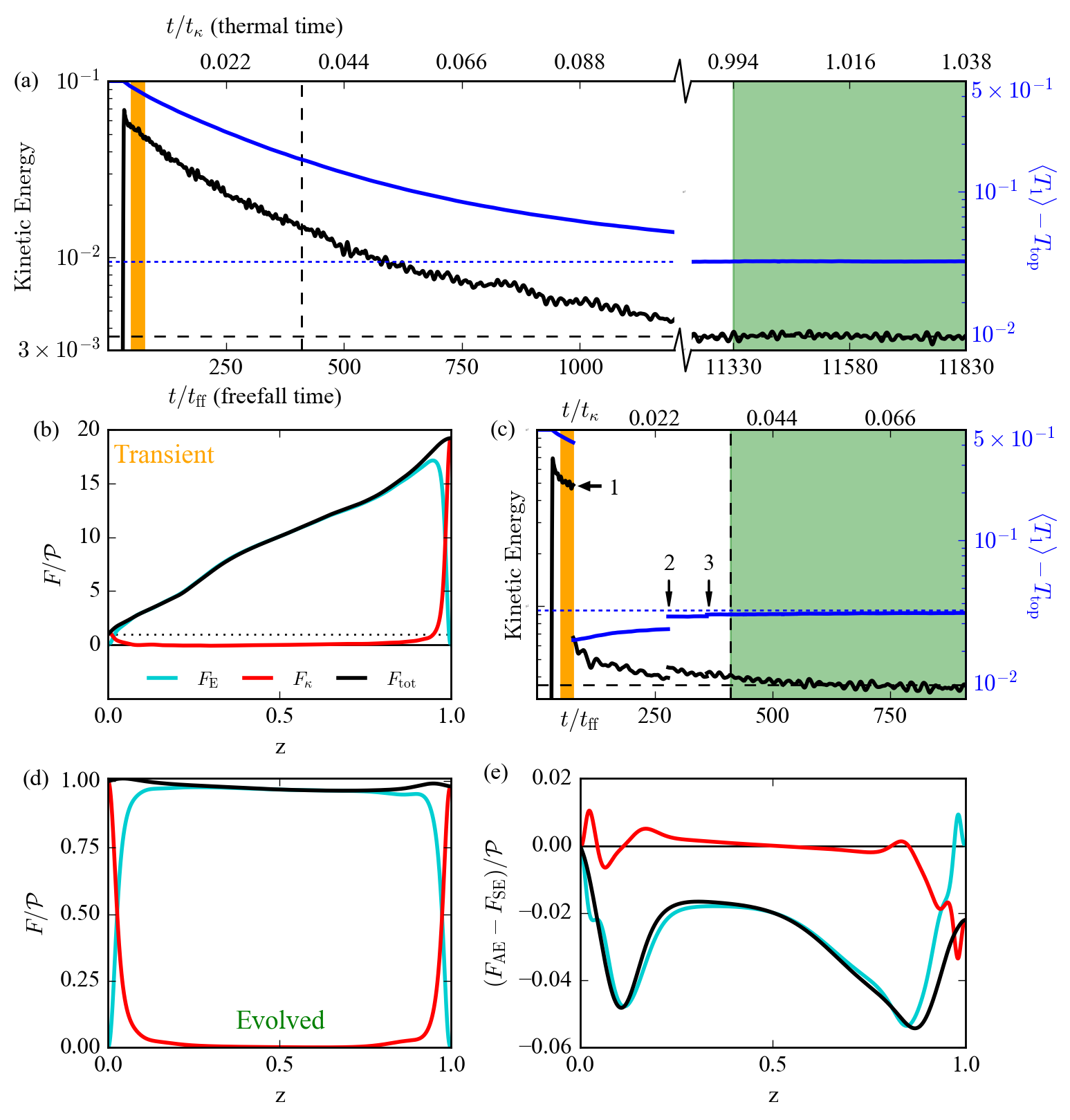
Figure 1: (a) Kinetic energy (black) and $\left\langle T\right\rangle-T_{\text{top}}$ (blue) vs. time are shown for a SE run at $S=10^{5}$. The mean evolved values of kinetic energy and mean temperature, averaged over the time shaded in green, are denoted by the horizontal dashed lines. (b) The time- and horizontally-averaged flux profiles are shown for the times highlighted in orange in (a). (c) The same quantities as in (a) are shown, but for AE at the same parameters. The axes are scaled identically in (a) and (c), and the AE method is used three times, marked by the numbered arrows. The fluxes averaged over the green shaded region of (c) are shown in (d). The difference between the fluxes in the AE and SE solutions is shown in (e).

In order to adjust the temperature profile to achieve AE, we calculate the total flux, F${}_{\text{tot}}=$ F${}_{\text{E}}$ + F_κ, and then derive the profiles

$$f_{\text{E}}(z)=\frac{\text{F}_{\text{E}}}{\text{F}_{\text{tot}}},\qquad f_{\kappa}(z)=\frac{\text{F}_{\kappa}}{\text{F}_{\text{tot}}},$$ (10)

which have the systematic asymmetries [Fig. 1(b)] removed. These profiles describe which parts of the atmosphere depend on convection to carry flux (where $f_{\text{E}}(z)=1$ and $f_{\kappa}(z)=0$). We presume that the early convection occupies roughly the same volume as the evolved convection, and thus that the extent of the early thermal boundary layers (where $f_{\kappa}(z)=1$ and $f_{\text{E}}(z)=0$) will not change significantly over the course of the atmosphere’s evolution. Under this assumption, in order to reach the converged state, the flux through the atmosphere must be decreased by some amount,

$$\xi(z,t)\equiv\frac{\text{F}_{\text{B}}}{\text{F}_{\text{tot}}},$$ (11)

where $\text{F}_{\text{B}}=\mathcal{P}$ is the amount of flux that enters the atmosphere at the bottom, fixed-flux boundary. For example, in Fig. 1b, F${}_{\text{tot}}\approx 19\mathcal{P}$ at the upper boundary, but in the relaxed state it should just be $\mathcal{P}$, so $\xi\approx 1/19$ at that depth.

To reduce the conductive flux by $\xi$, we examine the horizontally- and time-averaged Eqs. (5) and (6) in the time-stationary state; after neglecting terms which vanish due to symmetry, these equations become

$$\frac{\partial}{\partial z}\left\langle\varpi\right\rangle_{x,y}-\left\langle T_{1}\right\rangle_{x,y}\hat{z}=\left\langle\bm{u}\times\bm{\omega}\right\rangle_{x,y,\text{ ev}},$$ (12)

$$\frac{\partial}{\partial z}\text{F}_{\text{E, ev}}-\mathcal{P}\frac{\partial^{2}}{\partial z^{2}}\left\langle T_{1}\right\rangle_{x,y}=0.$$ (13)

Here, we construct $\text{F}_{\text{E, ev}}=\xi\text{F}_{\text{E}}$ and $\left\langle\bm{u}\times\bm{\omega}\right\rangle_{x,y,\text{ ev}}=\xi\left\langle\bm{u}\times\bm{\omega}\right\rangle_{x,y}$. Using these profiles and Eqs. (12) and (13), we solve for $\left\langle\varpi\right\rangle_{x,y}$ and $\left\langle T_{1}\right\rangle_{x,y}$. Our choice of fixing the temperature at the top boundary and the flux at the bottom boundary ensures that there is a unique solution for $\left\langle T_{1}\right\rangle_{x,y}$ given the evolved fluxes. If flux were fixed at both boundaries, there would be infinitely many temperature solutions. If temperature were fixed at both boundaries, $\text{F}_{\text{B}}$ would not be precisely known a priori.

Solving the above equations adjusts the mean thermal state and $\text{F}_{\kappa}$ of the atmosphere while leaving $\text{F}_{\text{E}}$ unchanged. In the bulk of the domain, convective enthalpy flux dominates transport, and so there we assume that $\text{F}_{\text{tot}}\approx\text{F}_{\text{E}}$. Upon removing terms which vanish due to symmetry, we note that the convective enthalpy flux is carried solely by the velocity field and perturbations in temperature away from the mean state, $\text{F}_{\text{E}}=\left\langle w(T_{1}-\left\langle T_{1}\right\rangle)\right\rangle$. In order to instantaneously decrease the convective enthalpy flux in a manner which is consistent with the conductive flux, we multiply both the velocity, $\bm{u}$, and temperature perturbations about the mean state, $T_{1}-\left\langle T_{1}\right\rangle_{x,y}$, by $\sqrt{\xi}$. This scaling of the velocity field is the reason that we multiply $\left\langle\bm{u}\times\bm{\omega}\right\rangle_{x,y}$, which is nondimensionally of order $u^{2}/L$, by $\xi$ while constructing $\left\langle\bm{u}\times\bm{\omega}\right\rangle_{x,y,\text{ ev}}$.

In general, the AE method occurs in the following steps. First, we pause a convective simulation and construct $\xi(z,t)$ from measured flux profiles in the convective domain. We solve a 1D boundary value problem (BVP) consisting of Eqs. (12) and (13) to obtain an evolved thermodynamic profile, and its corresponding conductive flux. We multiply both the temperature perturbations around the mean and the convective velocity flows by $\sqrt{\xi}$. After adjusing the fields of a simulation in this manner, we continue timestepping forward. For specifics on the precise implementation of the AE method, we refer the reader to appendix B.

IV Results

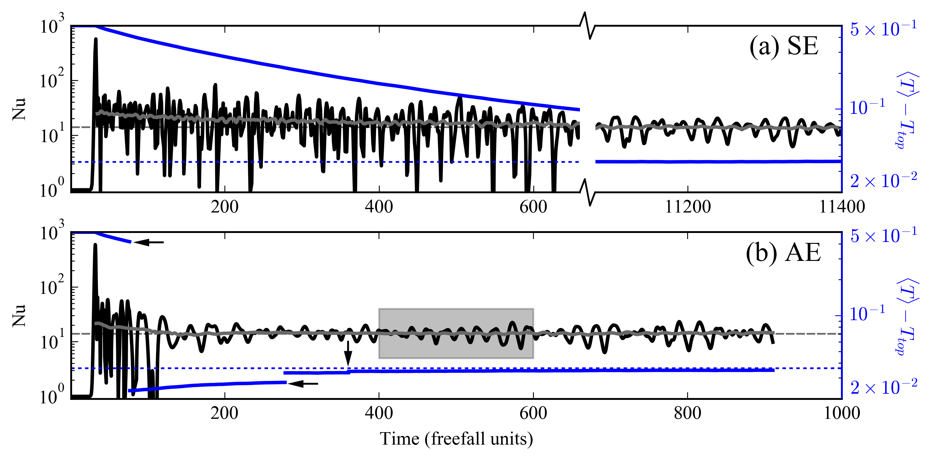
Figure 2: The time evolution of Nu (black) and $\left\langle T\right\rangle-T_{\text{top}}$ (blue) are shown for simulations at $S=10^{5}$ in SE (a) and AE (b). A moving average of Nu, using a centered boxcar with a span of 50 freefall time units, is overplotted as a gray line. We see that the mean value of Nu reaches its relaxed value quickly compared to $\left\langle T\right\rangle$. Regardless, fluctuations of Nu about the mean value are much smaller in the thermally relaxed state. The times at which AE solves occur are denoted by arrows in (b), and the gray boxed region is examined in more detail in Fig. 3.

We study evolved standard evolution (SE) solutions whose supercriticalities ($S$) are $S\in(1,10^{5}]$ in 2D and $S\in(1,10^{4}]$ in 3D. We compare their properties to accelerated evolution (AE) runs at $S\in(1,10^{7}]$ in 2D and $S\in(1,10^{4}]$ in 3D. We refer the reader to appendix A for a full list of simulations.

The Nusselt number (Nu) quantifies the efficiency of convective heat transport and is defined as

$$\text{Nu}=\frac{\left\langle F_{\text{conv}}+F_{\text{cond}}\right\rangle}{\left\langle F_{\text{cond, ref}}\right\rangle}=\frac{\left\langle wT-\mathcal{P}\partial_{z}T\right\rangle}{\left\langle-\mathcal{P}\partial_{z}T\right\rangle},$$ (14)

where the volume average of a quantity, $\eta$, is shown as $\left\langle\eta\right\rangle$. The time evolution of Nu in AE and SE is compared to the mean temperature evolution in Fig. 2. In Fig. 2(a), we show the evolution of the SE run at $S=10^{5}$. The black trace shows the instantaneous value of Nu, and the overplotted gray line shows a moving time average of Nu. The time average is taken using a centered boxcar window whose width is 50 $t_{\text{ff}}$. The mean value of Nu evolves towards its relaxed value (dashed horizontal gray line) rapidly compared to $\left\langle T\right\rangle-T_{\text{top}}$ (blue), which approaches its evolved state (dashed horizontal blue line) slowly. As such, it is possible to measure the statistically stationary mean value of Nu after only a few hundred simulated freefall times, as has been done previously Stevens et al. (2010). However, fluctuations in Nu around the mean value at early times have both a larger magnitude and higher frequency than the fluctuations in the relaxed state. In Fig. 2(b), we show the AE traces of Nu and $\left\langle T\right\rangle-T_{\text{top}}$ at $S=10^{5}$. The times at which AE solves occur are marked by arrows. Nu reaches its evolved mean value slightly more rapidly than in the SE case, and the frequency and magnitude of fluctuations in Nu away from the mean resemble the final relaxed state of SE.

When $S<10^{3.67}$ in 2D and for all runs in 3D, the evolved system is characterized by a time-stationary value of Nu, and is thus in a state of constant convective heat transport. At larger $S$ in 2D, the value of Nu varies significantly over time even in the relaxed state (as seen in Fig. 2). We examine the shaded region of Fig. 2(b) in more detail in the top left panel of Fig. 3, as well as a comparable time trace at $S=10^{7}$ (bottom, left panel). We find that these systems exhibit large Nu during states in which temperature fluctuations travel in their natural buoyant direction (Fig. 3, Ia and IIa, where cold elements fall and hot elements rise). However, when wrongly-signed temperature perturbations are entrained in an upflow or downflow with oppositely signed fluid, Nu is suppressed (Fig. 3, Ib and IIb, where warm fluid is pulled down by the downflow lane, and cool fluid is drawn up by the upflow lane). The plumes in these systems naturally oscillate horizontally over time, switching between transport being dominated by a counterclockwise cell, as pictured in Fig. 3, and a clockwise cell. Our choice of no-slip boundary conditions prevents the fluid from entering a full domain shearing state Goluskin et al. (2014), and the oscillatory motions of the plumes are a long-lived, stable phenomenon. However, thanks to our choice of periodic boundary conditions and despite the no-slip conditions, the full system of the upflow and downflow plumes is free to slowly migrate to the left or right over time, and we observe this phenomenon in our solutions. The 2D SE simulations exhibit the same horizontally oscillatory behavior as the AE solutions for the same initial conditions. This time-dependent behavior of Nu is not seen strongly in our 3D solutions, however most 3D simulations we conducted were at low $S$ compared to the runs in which this behavior was observed in 2D.

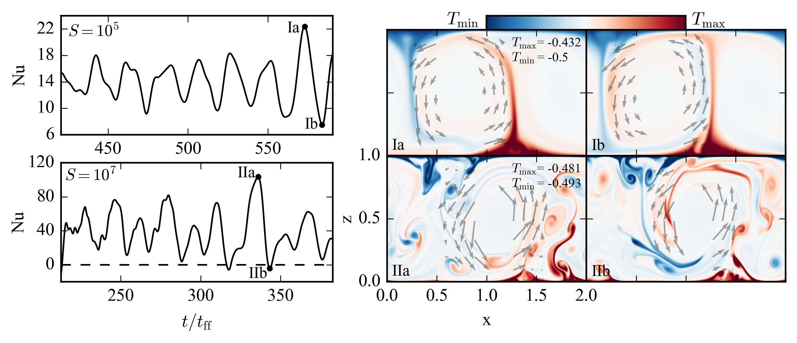
Figure 3: The time variation of the Nusselt number is shown for two AE cases at $S=10^{5}$ (top) and $S=10^{7}$ (bottom). On the left, the instantaneous value of Nu is shown as a function of time. On the right, temperature snapshots are shown for Nu maxima (Ia and IIa) and minima (Ib and IIb). The suppressed value of Nu at the minma arises from entrainment of fluid elements whose temperature perturbations are wrongly signed (e.g., hot material going downwards and cold material going upwards in Ib and IIb). The colorbar scaling of panels Ia&b are the same, as are the scalings of panels IIa&b. The minimum temperature is chosen by the fixed-temperature boundary condition at the top, $T_{\text{top}}=-0.5$. The decreased range of the colorbar scaling for for IIa&b was chosen to better display the convective dynamics.

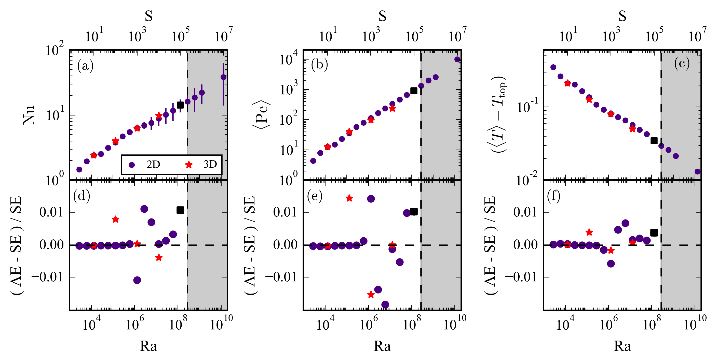
Figure 4: Volume- and time-averaged measurements of the Nusselt number (Nu), the RMS Peclet number ($\left\langle\text{Pe}\right\rangle$), and the mean temperature ($\left\langle T\right\rangle$) for AE runs are shown in (a)-(c). Symbols are located at the mean value of each measurement and denote 2D (purple circles) and 3D (red stars). The run at $S=10^{5}$ marked as a black square is examined in more detail in Figs. 1-3, 5, and 6. Vertical lines represent the standard deviation of the measurement, and quantify natural variation over the averaging window. (a) Nu scales as Ra^1/5; at high $S$ in 2D the value of Nu fluctuates over time (see Fig. 3). (b) Pe, which measures turbulence in the solution, scales as Ra^0.45. (c) The difference between $\left\langle T\right\rangle$ and the value of $T$ at the fixed-temperature top boundary is shown; this quantity scales as Ra^-1/5, the inverse of Nu. Relative error for measurements of (d) Nu, (e) Pe, and (f) $\left\langle T\right\rangle-T_{\text{top}}$ between AE solutions and SE solutions are shown. The greyed area of the plots indicates the region in which only AE runs were carried out due to computational expense.

The time- and volume-averaged values of Nu, the RMS Peclet number (Pe), and the mean temperature are shown for AE solutions in Figs. 4(a)-4(c). Mean values are shown by the symbols (purple circles and red stars), and the vertical lines represent the standard deviation of the measurement over time. Nu is shown as a function of Ra and $S$ in Fig. 4a, while $\text{Pe}=\left\langle|\bm{u}|\right\rangle/\mathcal{P}$ is shown in Fig. 4(b), and $\left\langle T\right\rangle-T_{\text{top}}$ (the mean temperature value minus its value at the upper, fixed temperature boundary) is shown in Fig. 4(c). We report $\text{Nu}\propto\text{Ra}^{1/5}$, $\text{Pe}\propto\text{Ra}^{0.45}$, and $(\left\langle T\right\rangle-T_{\text{top}})\propto\text{Ra}^{-1/5}$. The average temperature, $\left\langle T\right\rangle$, is dominated by its value in the isothermal interior, so this measurement serves as a probe of the temperature jump across the boundary layers. Thus, the inverse scaling of average temperature and Nu that we find here is expected for thermally equilibrated solutions Otero et al. (2002).

In Figs. 4(d)-4(f), we report the fractional difference between measurements in the AE and SE solutions. The mean values of Nu and $\left\langle T\right\rangle-T_{\text{top}}$ measured in AE are accurate to SE values to within $\sim 1$%. Pe measurements show marginally greater error, with AE measurements being $\leq 2$% different from SE measurements.

For the select 3D runs conducted in this study, the scaling of Nu, Pe, and $\left\langle T\right\rangle-T_{\text{top}}$ reported in Figs. 4(a)-4(c) is nearly identical to the 2D simulations. Errors between AE and SE solutions in 3D fall within the same range as errors in 2D in Figs. 4(d)-4(f). AE is therefore equally effective in both 2D and 3D, and we restrict much of our study to 2D here in order to more thoroughly sample parameter space.

The measurements presented in Fig. 4 demonstrate that AE can be powerfully employed in parameter space studies in which large numbers of simulations are compared in a volume-averaged sense. We now turn our examination to a more direct comparison of AE and SE for 2D convection at $S=10^{5}$, the time, flux, and Nu evolution of which are shown in Figs. 1, 2, and 3. All comparisons that follow for these two runs occur over the times shaded in green in Figs. 1(a) and 1(c). Measurements are sampled every 0.1 freefall time units for 500 total freefall time units.

As AE is fundamentally a 1D adjustment to the thermodynamic structure of the solution, we compare the horizontally- and time-averaged temperature profiles attained by AE and SE in Fig. 5(a). The boundary layer width and structure are nearly identical between the two solutions, but the the mean temperature in the isothermal interior differs by roughly 0.5% [Fig. 5(c)].

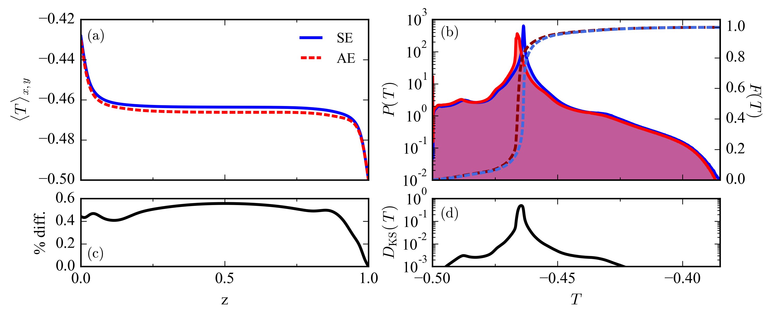
Figure 5: Comparisons of the evolved thermodynamic states of an AE and SE run at $S=10^{5}$ are shown. (a) Evolved horizontally- and time-averaged temperature profiles, as a function of height. (b) Probability Distribution Functions (PDFs, $P(T)$) and their integrated Cumulative Distribution Functions (CDFs, $F(T)$) of point-by-point measurements of the temperature field. (c) The percentage difference between the mean temperature profiles as a function of height. The difference between the mean profiles is very small, O(0.5%). (d) $D_{\text{KS}}(T)$, as defined in Eqn. 15, is shown. The small difference in the mean interior temperature between AE and SE results in a large difference between the two temperature distributions near the values of the temperature maxima. The spread of temperature around the maxima, which includes the fluctuations that drive convection, are nearly identical between the two runs.

The probability distribution functions (PDFs) of point-by-point temperature measurements are compared for the two runs in Fig. 5(b). To construct these PDFs, we interpolate the full temperature field at each measurement time onto an evenly spaced grid, determine the frequency distribution of all $T$ values over the duration of the 500 $t_{\text{ff}}$ measurement window, and then normalize the distribution such that its integral is unity. The two PDFs have noticeably different maxima, as is expected from Fig. 5(a). Over long timescales, the 0.5% difference between the two profiles would disappear, as the AE solution evolves to be exactly the SE solution; this is evident in the asymmetry of the AE PDF near the maxima in Fig. 5(b) and also the trend of the mean temperature over time in Fig. 1(c).

One method of comparing two PDFs to determine if they are drawn from the same underlying sample distribution is through the use of a Kolmogorov-Smirnov ($D_{\text{KS}}$) test Wall and Jenkins (2012). We calculate the $D_{\text{KS}}$ statistic for a PDF of some value, $q$, as

$$D_{\text{KS}}(q)=F_{\text{AE}}(q)-F_{\text{SE}}(q),$$ (15)

where $F$ stands for cumulative distribution function (CDF), the integral of the PDF. A traditional Kolmogorov-Smirnov statistic is just a single value, $\overline{D_{\text{KS}}(q)}=|D_{\text{KS}}(q)|_{\infty}=\text{max}|D_{\text{KS}}(q)|$, and we use both the profile KS$(q)$ and $\overline{D_{\text{KS}}(q)}$ to gain insight into the likeness of two PDFs. We show $D_{\text{KS}}(T)$ in Fig. 5(d), and the CDFs used to construct it overlay the PDFs in Fig. 5(b). Near the maxima of the temperature PDFs, $\overline{D_{\text{KS}}(T)}=0.495$, which is very large and implies that roughly half of all measurements in the AE case are at a lower $T$ than those in the SE case. While this difference is significant, it is also expected from Fig. 5(a). Fortunately, $D_{\text{KS}}(T)$ is very small away from the maxima, indicating that the temperature fluctuations off of the maxima, which are the primary drivers of convective transport, are nearly identical.

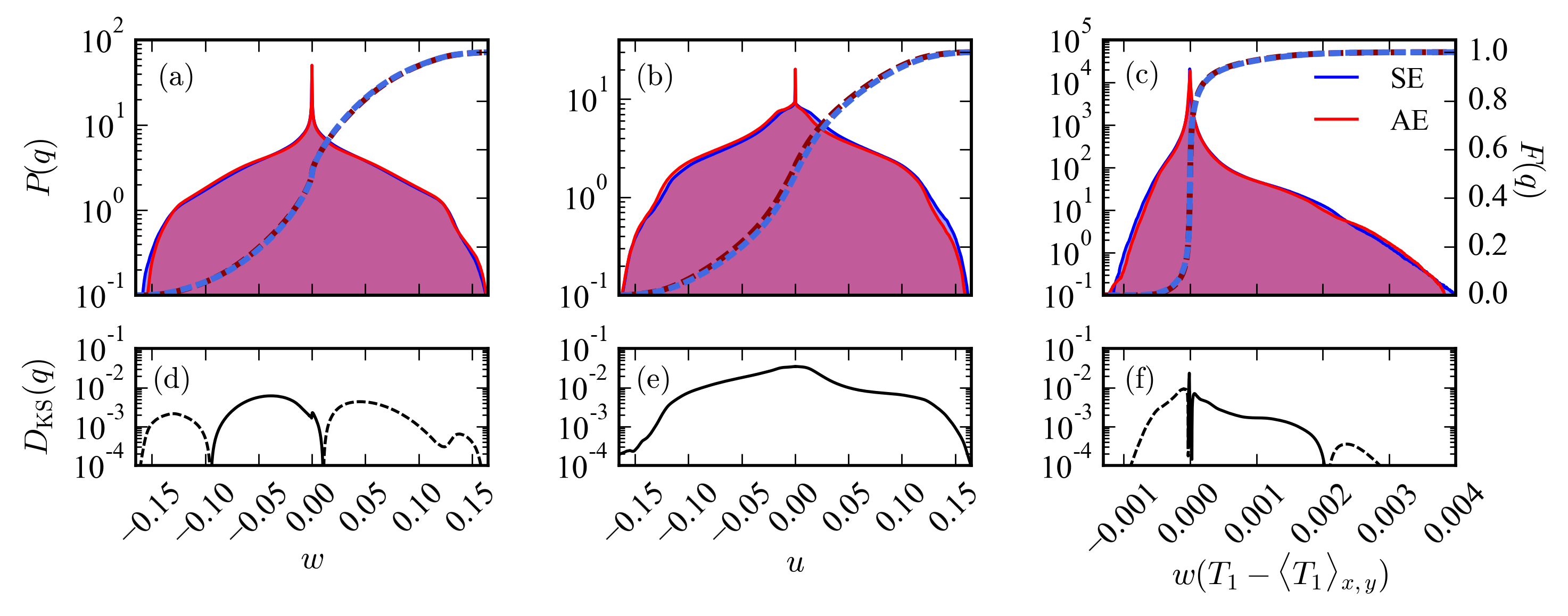
Figure 6: Probability distribution functions (PDFs, $P(q)$) of (a) the vertical velocity ($q=w$), (b) the horizontal velocity ($q=u$), and (c) nonlinear convective transport [$q=w(T_{1}-\left\langle T_{1}\right\rangle_{x,y})$] are shown for 2D runs achieved through SE (blue) and AE (red) at $S=10^{5}$. The cumulative distribution function (CDF) is overplotted for each PDF. (d-f) The $D_{\text{KS}}$ profiles, as defined in Eq. (15), are shown for the related distributions; solid lines indicate positive values while dashed lines are negative values. Unlike the temperature distributions in Fig. 5, these distributions show very good agreement and small values of the $D_{\text{KS}}$ statistic.

In addition to adjusting the 1D thermal profile, the AE method also scales the simulation velocities and temperature fluctuations by $\sqrt{\xi}$. In Fig. 6 we examine the velocities and heat transport found in the evolved states. Shown are the PDFs of vertical velocity [$w$, Fig. 6(a)], horizontal velocity [$u$, Fig. 6(b)], and the nonlinear vertical convective flux [$w(T_{1}-\left\langle T_{1}\right\rangle_{x,y})$, Fig. 6(c)]. Each PDF here shows a strong peak near zero due to the no-slip, impenetrable velocity boundary conditions (Eq. (8)). The CDFs of each profile are overplotted, and corresponding KS profiles are shown in Figs. 6(d)-6(f). We report $\overline{D_{\text{KS}}(w)}=0.00615$, $\overline{D_{\text{KS}}(u)}=0.0349$, and $\overline{D_{\text{KS}}(w(T_{1}-\left\langle T_{1}\right\rangle_{x,y}))}=0.0263$. The difference in vertical velocity and heat transport between AE and SE is negligible, which is unsurprising in light of the Nu measurements of Figs. 4(a) and 4(d). This also confirms that the large $\overline{D_{\text{KS}}(T)}$ in Fig. 5(d) is not of concern, and that the AE run achieves the same relaxed convective solution as the SE run. We find that the difference in $D_{\text{KS}}(u)$, which consistently has more probability of flows moving left (in the -$x$ direction), appears to be caused by a more prominent migration of the full roll system in the -$x$ direction in the AE run than in the SE run. This migration does not appear to affect the vertical transport appreciably.

V Computational Time-savings of AE

Table 1: Shown are details regarding the computational cost of select AE and SE runs in 2D and 3D. The supercriticality ($S$), coefficient resolution (nz, nx, ny), number of CPUs used to perform the calculation ($N_{\text{CPU}}$), number of CPU-hours used to perform the run ($t_{\text{CPU,AE/SE}}$), and ratio of CPU-hours used in the AE run compared to the SE run are provided.

$S$	nz$\times$nx$\times$ny	$N_{\text{CPU}}$	$t_{\text{CPU, SE}}$	$t_{\text{CPU, AE}}$	$t_{\text{CPU,AE}}/t_{\text{CPU,SE}}$
2D Runs
$10^{2}$	64$\times$128	32	2.2	4.4	2.0
$10^{3}$	128$\times$256	64	53	21	0.39
$10^{4}$	256$\times$512	128	1.2$\times 10^{3}$	1.8$\times 10^{2}$	0.15
$10^{5}$	512$\times$1024	256	2.4$\times 10^{4}$	2.8$\times 10^{3}$	0.12
3D Runs
$10^{1}$	32$\times$64$\times$64	512	62	1.1$\times 10^{2}$	1.7
$10^{2}$	64$\times$128$\times$128	512	1.9$\times 10^{2}$	1.1$\times 10^{2}$	0.60
$10^{3}$	128$\times$256$\times$256	2048	7.0$\times 10^{3}$	1.4$\times 10^{3}$	0.20
$10^{4}$	256$\times$512$\times$512	8192	3.3$\times 10^{5}$	2.3$\times 10^{4}$	0.070

Computational time-saving is the primary reason to use AE rather than evolving all solutions through SE. In table 1, we compare cpu-hour cost for select 2D and 3D runs in which both AE and SE solutions were computed. Times reported for AE and SE runs only include the time required to reach a relaxed state, and do not include the time over which measurements were taken in that state (e.g., the green shaded regions of Figs. 1(a) and 1(c) are not included in the $S=10^{5}$ times). All simulations were performed on Broadwell nodes on NASA’s Pleiades supercomputer (Intel Xeon E5-2680v4 processors). The key metric which highlights the usefulness of AE is the number of cpu-hours used for the AE run divided by cpu-hours used for the SE run ($t_{\text{CPU,AE}}/t_{\text{CPU,SE}}$). We see that at low resolution and low supercriticality, $t_{\text{CPU,AE}}/t_{\text{CPU,SE}}>1$, and AE is not useful. However, as $S$ grows, $t_{\text{CPU,AE}}/t_{\text{CPU,SE}}$ shrinks. At the highest supercriticalities for which AE and SE were compared in this work, AE runs cost roughly an order of magnitude less computing time than SE runs.

Integrating information about the mean state in time (fluxes, etc.) decreases the rate at which our solver timesteps early in the AE cases. However, the first application of AE in a given simulation [e.g., Fig. 1(c), at the arrow labeled “1”] drastically increases the average timestep by fastforwarding the simulation into a more stable state with lower convective velocities. For the $S=10^{5}$ case we examined in detail, the average time step grew by a factor of 2-3. At $S=10^{7}$, the AE solve immediately improved the timestep size by nearly a factor of 4.

VI Discussion & Conclusions

In this work we have studied a method of Accelerated Evolution (AE) which can be employed to achieve rapid thermal relaxation of convective simulations. We compared this technique to the Standard Evolution (SE) of convection through a full thermal diffusion timescale, and we showed that AE rapidly obtains solutions whose dynamics are statistically similar to SE solutions. The AE method is valid at low values of $S$, where SE solutions converge quickly due to the short thermal timescale, and AE remains applicable at high values of $S$, where SE solutions are intractable. As discussed, AE is equally applicable in 2D and 3D; here we have restricted most of our study to 2D to extend our parameter space coverage. At the largest values of $S$ in which AE and SE are compared in this work, we find time savings of nearly an order of magnitude.

Here we studied the simplest possible case for the application of AE: Rayleigh-Bénard convection at low aspect ratio with mixed thermal boundary conditions. We anticipate that this technique will be powerful in its extensions to more complicated studies. To achieve AE in more complicated systems, one need only derive the steady-state, horizontally-averaged equations governing the convective dynamics [e.g., the analogs to Eqs. (12) and (13)] and couple those equations with knowledge of the boundary conditions and current dynamics as described in Sec. III and appendix B. In general, AE should be useful in studies where there are two disparate timescales which must both be resolved and which cannot be overcome through clever timestepping techniques. Some avenues in which extensions of AE could be beneficial for expanding the available parameter space of exploration include studies of internally heated convection Goluskin (2016), convection with height-dependent conductivities Käpylä et al. (2017), penetrative convection Hurlburt et al. (1986); Brandenburg et al. (2005); Couston et al. (2017), or fully compressible, stratified convection Anders and Brown (2017). As AE is fundamentally a horizontally uniform adjustment to the thermodynamic structure of the convective domain, it is unlikely that these techniques should be applied straightforwardly to nonperiodic convective domains.

We conclude by noting that AE should be extended to these more complicated studies with caution. While AE was extremely effective in this simple case studied here (where the aspect ratio was low, the bounds of the convective domain were pre-defined, and the solutions were simple rolls), this may not be the case for more complicated systems. For example, at higher aspect ratios, multiple stable solution branches may exist, and there is no guarantee that AE and SE will arrive at the same solution. Some assumptions which inform the AE solution, such as the assumption that the convection intially occupies the same space as the evolved convection, may not hold in studies of penetrative convection, despite the fact that similar methods have long been used in those studies Hurlburt et al. (1986). Extensions to fully compressible convection in which there are two true thermodynamic variables Anders and Brown (2017) must contain a very careful treatment of AE pressure adjustments, so as to avoid wave-launching pressure mismatches. Our work here serves as a basis for determining if AE techniques are effective in more complex studies of convection.

Appendix A Table of Runs

In Table 2 we list key properties of all simulations conducted in this work.

Table 2: Simulation parameters. We report the supercriticality ($S$), Rayleigh number (Ra), and coefficient resolution (nz, nx, and ny are the number of coefficients in the z, x, and y directions respectively). Simulation run times required to reach convergence are reported for the SE solutions ($t_{\text{SE}}$) and the AE solutions ($t_{\text{AE}}$). The amount of time over which simulations measurements were taken in the evolved state is listed ($t_{\text{avg}}$). All times are in freefall time units. The volume-averaged Nusselt number (Nu) of the AE and SE solutions are shown. In the upper part of the table, information pertaining to 2D runs is reported, while information pertaining to 3D runs is in the lower part of the table.

$S$	Ra	nz$\times$nx$\times$ny	$t_{\text{SE}}$	$t_{\text{AE}}$	$t_{\text{avg}}$	Nu${}_{\text{SE}}$	Nu${}_{\text{AE}}$
2D Runs
$10^{1/3}$	$2.79\times 10^{3}$	32$\times$64	$52.8$	$340$	100	1.46	1.46
$10^{2/3}$	$6.01\times 10^{3}$	32$\times$64	$77.6$	$282$	100	1.95	1.95
$10^{1}$	$1.30\times 10^{4}$	32$\times$64	$114$	$265$	100	2.43	2.42
$10^{1+1/3}$	$2.79\times 10^{4}$	32$\times$64	$167$	$251$	100	2.54	2.54
$10^{1+2/3}$	$6.01\times 10^{4}$	32$\times$64	$245$	$245$	100	3.14	3.14
$10^{2}$	$1.30\times 10^{5}$	64$\times$128	$360$	$326$	100	3.8	3.8
$10^{2+1/3}$	$2.79\times 10^{5}$	64$\times$128	$528$	$248$	100	4.71	4.71
$10^{2+2/3}$	$6.01\times 10^{5}$	64$\times$128	$776$	$251$	100	5.5	5.5
$10^{3}$	$1.30\times 10^{6}$	128$\times$256	$1.14\times 10^{3}$	$268$	200	6.4	6.33
$10^{3+1/3}$	$2.79\times 10^{6}$	128$\times$256	$1.67\times 10^{3}$	$247$	500	6.87	6.95
$10^{3+2/3}$	$6.01\times 10^{6}$	256$\times$512	$2.45\times 10^{3}$	$275$	500	7.54	7.59
$10^{4}$	$1.30\times 10^{7}$	256$\times$512	$3.60\times 10^{3}$	$301$	500	8.83	8.83
$10^{4+1/3}$	$2.79\times 10^{7}$	256$\times$512	$5.28\times 10^{3}$	$317$	500	10.13	10.14
$10^{4+2/3}$	$6.01\times 10^{7}$	256$\times$512	$7.76\times 10^{3}$	$326$	500	11.65	11.69
$10^{5}$	$1.30\times 10^{8}$	512$\times$1024	$1.14\times 10^{4}$	$411$	500	14.02	14.18
$10^{5+1/3}$	$2.79\times 10^{8}$	512$\times$1024	$1.67\times 10^{4}$	$391$	500	—	16.21
$10^{5+2/3}$	$6.01\times 10^{8}$	512$\times$1024	$2.45\times 10^{4}$	$453$	500	—	18.58
$10^{6}$	$1.30\times 10^{9}$	1024$\times$2048	$3.60\times 10^{4}$	$436$	500	—	22.13
$10^{7}$	$1.30\times 10^{10}$	2048$\times$4096	$1.14\times 10^{5}$	$183$	170	—	38.29
3D Runs
$10^{1}$	$1.30\times 10^{4}$	32$\times$64$\times$64	$114$	$261$	100	2.42	2.42
$10^{2}$	$1.30\times 10^{5}$	64$\times$128$\times$128	$360$	$249$	100	3.97	4
$10^{3}$	$1.30\times 10^{6}$	128$\times$256$\times$256	$1.14\times 10^{3}$	$243$	500	6.27	6.27
$10^{4}$	$1.30\times 10^{7}$	256$\times$512$\times$512	$3.60\times 10^{3}$	$244$	500	9.92	9.88

Appendix B Accelerated Evolution Recipe

In order to achieve Accelerated Evolution (AE), we pause the Direct Numerical Simulation (DNS) which is evolving the dynamics of convection and solve a 1D Boundary Value Problem (BVP) consisting of Eqns. (12) & (13). After solving this BVP, we appropriately adjust the fields being evolved in the DNS towards their evolved state, and then we continue running the now-evolved DNS. The specific steps taken in completing the AE method are as follows:

1. Wait some time, $t_{\text{transient}}$, before beginning the AE process.

2. During the DNS, calculate time averages of the 1D vertical profiles of F${}_{\text{E}}$, F${}_{\text{tot}}$, and $\left\langle\bm{u}\times\bm{\omega}\right\rangle_{x,y}$, updating them every timestep. To calculate these averages, we use a trapezoidal-rule integration in time, and then divide by the total time elapsed over which the average is taken.

3. Pause the DNS once the averages are sufficiently converged. To ensure that an average is converged, at least some time $t_{\text{min}}$ must have passed since the average was started to ensure that the full range of convective dynamics are probed, and the profiles must change by no more than $P$% on a given timestep.

4. Construct $\xi$, F${}_{\text{E, ev}}$, and $\left\langle\bm{u}\times\bm{\omega}\right\rangle_{x,y\text{, ev}}$, as specified in Sec. III from the averaged profiles.

5. Solve the BVP for $\left\langle T_{1}\right\rangle_{x,y}$ and $\left\langle\varpi\right\rangle_{x,y}$ of the evolved state. Set the horizontal average of the current DNS thermodynamic fields equal to the results of the BVP.

6. Multiply the velocity field, $\bm{u}=u\hat{x}+v\hat{y}+w\hat{z}$, and the temperature fluctuations, $T-\left\langle T\right\rangle_{x,y}$, by $\sqrt{\xi}$ in the DNS to properly reduce the convective flux.

7. Continue running the DNS.

We refer to this process as an “AE BVP solve.”

While the use of a single AE BVP solve rapidly advances the convecting state to one that is closer to the relaxed state, we find that repeating this method multiple times is the best way to ensure that the AE solution is truly converged. For all runs in 2D at $S<10^{5}$, we set $t_{\text{transient}}=50$, completed an AE BVP solve with $t_{\text{min}}=30$ and $P=0.1$, and then repeated the procedure. For all 3D runs and 2D runs with $S\in[10^{5},10^{6}]$, we did a first AE BVP solve with $t_{\text{transient}}=20$, $t_{\text{min}}=20$, and $P=1$ in order to quickly reach a near- converged state and vastly increase our timestep size. After this first solve, we completed two AE BVP solves, with $t_{\text{transient}}=30$, $t_{\text{min}}=30$, and $P=0.1$ to get very close to the solution (as in Fig. 1c). At very high $S=10^{7}$, we ran two AE BVP solves with $t_{\text{min}}=20$ and $P=1$. For the first solve, we set $t_{\text{transient}}=20$, and for the second we set $t_{\text{transient}}=30$. We used fewer solves at this high value of $S$ in part to reduce the computational expense of the run, and in part because a third BVP generally did not greatly alter the solution (as in Fig. 1c, arrow 3). We wait 50 freefall times after the final AE BVP solve of each run before beginning to take measurements.

In general, to use AE, a threshold, $f$, should be chosen. When the fractional change of the mean temperature profile from an AE BVP solve becomes less than $f$, the solution can be considered converged on its chosen solution branch. In other words, once

$$\frac{|\left\langle T\right\rangle_{\text{DNS}}-\left\langle T\right\rangle_{\text{AE}}|}{|\left\langle T\right\rangle_{\text{DNS}}|}<f,$$ (16)

the solution is converged. In this work, we chose our number of AE iterations such that $f\approx 10^{-2}$. In general, the user of AE could set $f$ smaller, and in doing so reduce the separation between the AE and SE solutions, which can be seen in e.g., Fig. 5a&b. However, smaller values of $f$ require additional AE BVP solves, and likely require smaller values of $P$, resulting in longer wait times while the horizontal averages are computed.

References

- Brown et al. (2010) B. P. Brown, M. K. Browning, A. S. Brun, M. S. Miesch, and J. Toomre, “Persistent Magnetic Wreaths in a Rapidly Rotating Sun,” Astrophys. J. 711, 424–438 (2010), arXiv:1011.2831 [astro-ph.SR] .
- Featherstone and Hindman (2016) N. A. Featherstone and B. W. Hindman, “The Spectral Amplitude of Stellar Convection and Its Scaling in the High-Rayleigh-number Regime,” Astrophys. J. 818, 32 (2016), arXiv:1511.02396 [astro-ph.SR] .
- Viallet et al. (2011) M. Viallet, I. Baraffe, and R. Walder, “Towards a new generation of multi-dimensional stellar evolution models: development of an implicit hydrodynamic code,” Astronomy & Astrophysics 531, A86 (2011), arXiv:1103.1524 [astro-ph.IM] .
- Viallet et al. (2013) M. Viallet, I. Baraffe, and R. Walder, “Comparison of different nonlinear solvers for 2D time-implicit stellar hydrodynamics,” Astronomy & Astrophysics 555, A81 (2013), arXiv:1305.6581 [astro-ph.SR] .
- Viallet et al. (2016) M. Viallet, T. Goffrey, I. Baraffe, D. Folini, C. Geroux, M. V. Popov, J. Pratt, and R. Walder, “A Jacobian-free Newton-Krylov method for time-implicit multidimensional hydrodynamics. Physics-based preconditioning for sound waves and thermal diffusion,” Astronomy & Astrophysics 586, A153 (2016), arXiv:1512.03662 [astro-ph.IM] .
- Lecoanet et al. (2014) D. Lecoanet, B. P. Brown, E. G. Zweibel, K. J. Burns, J. S. Oishi, and G. M. Vasil, “Conduction in Low Mach Number Flows. I. Linear and Weakly Nonlinear Regimes,” Astrophys. J. 797, 94 (2014), arXiv:1410.5424 [astro-ph.SR] .
- Anders and Brown (2017) E. H. Anders and B. P. Brown, “Convective heat transport in stratified atmospheres at low and high Mach number,” Physical Review Fluids 2, 083501 (2017), arXiv:1611.06580 [physics.flu-dyn] .
- Bordwell et al. (2018) B. Bordwell, B. P. Brown, and J. S. Oishi, “Convective Dynamics and Disequilibrium Chemistry in the Atmospheres of Giant Planets and Brown Dwarfs,” Astrophys. J. 854, 8 (2018), arXiv:1802.03026 [astro-ph.EP] .
- Stix (2003) M. Stix, “On the time scale of energy transport in the sun,” Solar Physics 212, 3–6 (2003).
- Johnston and Doering (2009) H. Johnston and C. R. Doering, “Comparison of Turbulent Thermal Convection between Conditions of Constant Temperature and Constant Flux,” Phys. Rev. Lett. 102, 064501 (2009), arXiv:0811.0401 [physics.flu-dyn] .
- Verzicco and Camussi (1997) R. Verzicco and R. Camussi, “Transitional regimes of low-Prandtl thermal convection in a cylindrical cell,” Physics of Fluids 9, 1287–1295 (1997).
- Hurlburt et al. (1984) N. E. Hurlburt, J. Toomre, and J. M. Massaguer, “Two-dimensional compressible convection extending over multiple scale heights,” Astrophys. J. 282, 557–573 (1984).
- Couston et al. (2017) L.-A. Couston, D. Lecoanet, B. Favier, and M. Le Bars, “Dynamics of mixed convective-stably-stratified fluids,” Physical Review Fluids 2, 094804 (2017), arXiv:1709.06454 [physics.flu-dyn] .
- Brandenburg et al. (2005) A. Brandenburg, K. L. Chan, Å. Nordlund, and R. F. Stein, “Effect of the radiative background flux in convection,” Astronomische Nachrichten 326, 681–692 (2005), astro-ph/0508404 .
- Stevens et al. (2011) R. J. A. M. Stevens, D. Lohse, and R. Verzicco, “Prandtl and Rayleigh number dependence of heat transport in high Rayleigh number thermal convection,” Journal of Fluid Mechanics 688, 31–43 (2011), arXiv:1102.2307 [physics.flu-dyn] .
- Julien et al. (1998) Keith Julien, Edgar Knobloch, and Joseph Werne, “A New Class of Equations for Rotationally Constrained Flows,” Theoretical and Computational Fluid Dynamics 11, 251–261 (1998).
- Sprague et al. (2006) Michael Sprague, Keith Julien, Edgar Knobloch, and Joseph Werne, “Numerical simulation of an asymptotically reduced system for rotationally constrained convection,” Journal of Fluid Mechanics 551, 141–174 (2006).
- Hurlburt et al. (1986) N. E. Hurlburt, J. Toomre, and J. M. Massaguer, “Nonlinear compressible convection penetrating into stable layers and producing internal gravity waves,” Astrophys. J. 311, 563–577 (1986).
- Spiegel and Veronis (1960) E. A. Spiegel and G. Veronis, “On the Boussinesq Approximation for a Compressible Fluid.” Astrophys. J. 131, 442 (1960).
- Burns et al. (2016) K. Burns, G. Vasil, J. Oishi, D. Lecoanet, and B. Brown, “Dedalus: Flexible framework for spectrally solving differential equations,” Astrophysics Source Code Library (2016), ascl:1603.015 .
- Ascher et al. (1997) U. M. Ascher, S. J. Ruuth, and R. J. Spiteri, “Implicit-explicit Runge-Kutta methods for time-dependent partial differential equations,” Applied Numerical Mathematics 25, 151–167 (1997).
- (22) See Supplemental Material at [URL] for a .zip file of the python run scripts used to perform all simulations in this work. This code was run using the Dedalus mercurial repository (https://bitbucket.org/dedalus-project/dedalus/src/default/) at commit node ID dab6af2abaab03c059a4e9513f6a4d98320c2f02.
- Goluskin et al. (2014) David Goluskin, Hans Johnston, Glenn R. Flierl, and Edward A. Spiegel, “Convectively driven shear and decreased heat flux,” J. Fluid Mech. 759, 360–385 (2014).
- Goluskin (2016) David Goluskin, Internally Heated Convection and Rayleigh-Bénard Convection (Springer International Publishing, 2016).
- Cattaneo et al. (1991) F. Cattaneo, N. H. Brummell, J. Toomre, A. Malagoli, and N. E. Hurlburt, “Turbulent compressible convection,” Astrophys. J. 370, 282–294 (1991).
- Korre et al. (2017) L. Korre, N. Brummell, and P. Garaud, “Weakly non-Boussinesq convection in a gaseous spherical shell,” Phys. Rev. E 96, 033104 (2017), arXiv:1704.00817 [physics.flu-dyn] .
- Stevens et al. (2010) Richard J. A. M. Stevens, Roberto Verzicco, and Detlef Lohse, “Radial boundary layer structure and Nusselt number in Rayleigh-Bénard convection,” Journal of Fluid Mechanics 643, 495–507 (2010).
- Otero et al. (2002) J. Otero, R. W. Wittenberg, R. A. Worthing, and C. R. Doering, “Bounds on Rayleigh Bénard convection with an imposed heat flux,” J. Fluid Mech. 473, 191–199 (2002).
- Wall and Jenkins (2012) J. V. Wall and C. R. Jenkins, Practical Statistics for Astronomers, by J. V. Wall , C. R. Jenkins, Cambridge, UK: Cambridge University Press, 2012 (2012).
- Käpylä et al. (2017) P. J. Käpylä, M. Rheinhardt, A. Brandenburg, R. Arlt, M. J. Käpylä, A. Lagg, N. Olspert, and J. Warnecke, “Extended Subadiabatic Layer in Simulations of Overshooting Convection,” Astrophys. J. Lett. 845, L23 (2017), arXiv:1703.06845 [astro-ph.SR] .