Expressive power of outer product manifolds on feed-forward neural networks

Abstract

Hierarchical neural networks are exponentially more efficient than their corresponding “shallow” counterpart with the same expressive power, but involve huge number of parameters and require tedious amounts of training. Our main idea is to mathematically understand and describe the hierarchical structure of feedforward neural networks by reparametrization invariant Riemannian metrics. By computing or approximating the tangent subspace, we better utilize the original network via sparse representations that enables switching to shallow networks after a very early training stage. Our experiments show that the proposed approximation of the metric improves and sometimes even surpasses the achievable performance of the original network significantly even after a few epochs of training the original feedforward network.

1 Introduction

Hierarchical neural networks are among the most important machine learning models and are deemed to be the state-of-the-art models in problems like image classification Szegedy et al., (2016); He et al., (2016), various natural language processing problems Greff et al., (2017), object detection Ren et al., (2015), image captioning Vinyals et al., (2017) or reinforcement learning Silver et al., (2017). There are several challenges that are related to the generalizational power, the expressive power Bartlett and Maass, (2003); Zhang et al., 2016a ; Lin and Tegmark, (2016); Rolnick and Tegmark, (2017); Bengio and Delalleau, (2011); Kirkpatrick et al., (2017), the efficiency, Szegedy et al., (2016); He et al., (2016); Greff et al., (2017); Kingma and Welling, (2013); Goodfellow et al., (2014); Ren et al., (2015) and the optimization methods Ioffe and Szegedy, (2015); Srivastava et al., (2014); Amari, (1996); Kingma and Ba, (2014); Ollivier, (2015) of these models.

Inference for feed-forward neural networks with common, almost everywhere continuously differentiable cost and activation functions are usually trainable via the partial derivatives of the loss function respect to the parameters of the network Rumelhart et al., (1985), using some sort of regularization method Kingma and Ba, (2014); Zeiler, (2012); Srivastava et al., (2014); Ioffe and Szegedy, (2015). As a common choice, training algorithms use back-propagation on mini batches to estimate the first and second order gradient Nesterov, (1983); Amari, (1996); Kingma and Ba, (2014). The non-convex nature of the loss functions of feed-forward neural networks makes simple gradient based learning methods result in convergence to a local minimum instead of a global one. There are some refined ideas to overcome this serious issue. For example DropOut Srivastava et al., (2014) may make the model “jump” out of local minima with non-zero probability, although at the same time it can make it “jump” away from the global minimum too. The second order derivatives form the Hessian matrix Shima, (1995); Amari and Armstrong, (2014) and are used as the normalization part of the “Newtonian” gradient.

In the paper, we investigate the connection between the structure of a neural network and Riemannian manifolds to gain a better understanding and to utilize more of their potential. In a way, many of the existing machine learning problems can be investigated as statistical learning problems. Although information geometry Amari, (1996) plays an important role in statistical learning, the geometrical properties of target functions both widely used and recently discovered, along with those of the models themselves, are not well studied.

Over the parameter space and the error function we can often determine a smooth manifold Ollivier, (2015). In this paper we investigate the tangent bundle of this manifold in order to understand the behavior of certain networks better and to take advantage of specific Riemannian metrics having unique invariance properties C̆encov, (1982); Campbell, (1986). This approach may tell us more about what a neural network can and cannot express Lin and Tegmark, (2016). We aim to understand how the chosen learning algorithm, target function and the complexity of the chosen model determine the geometrical properties of the underlying manifolds. This knowledge might allow us to determine the achievable approximation and estimation error of a model before finishing its training.

We consider various smooth manifolds on the parameter space derived from the error function and examine some Hessian based Riemannian metrics. We use the partial derivatives in the tangent space as representation of data points. The inner products in the tangent space are quadratic, therefore if we separate the samples with a second order polynomial, then the actual metric will be irrelevant.

Our contributions are the following.

• We prove that a class of Riemannian metrics called the outer product metrics on feed-forward discriminative and generative neural networks are invariant to reparametrization and the inner product is sub quadratic. Hence the inner product can be used to optimize a weakly trained NN.

• We describe an approximation algorithm for the inner product space, in case of weekly trained NNs of various sparsities.

• We give heuristics for classification tasks where the coefficients of the monomials in the inner product are not necessarily determined.

Our experiments were done on the CIFAR-10 Krizhevsky, (2009) and MNIST (LeCun and Cortes,, 2010) data sets. We showed that if we determine the extended Hessian manifold in an early stage of learning of the underlying feed-forward neural network (after only a few epochs), we can outperform the fully trained network by passing the linearized inner product space to a shallow network.

2 Related work

Feed-forward neural networks are described in Bishop, (1992); Zhang et al., 2016a ; Rolnick and Tegmark, (2017); Lin and Tegmark, (2016). Bengio et al. consider a feed-forward neural network deep if the number of hidden layers is more than one Bengio and Delalleau, (2011). The most common layer types are the fully connected and the convolutional layer while the most popular activation functions (which are the non-linear functions applied to the linear combination of the preceding layer’s activations), are sigmoid, hyperbolic tangent (tanh) or some variant of the rectified linear unit (ReLU). In case of discriminative models, the activation function of the output layer is usually softmax.

To determine the parameters of a network, some form of gradient descent is used. Back-propagation was introduced in Rumelhart et al., (1985) and even simple regularization Krogh and Hertz, (1992) plays an important role during training. The problem of “vanishing gradients” became a serious issue in recurrent neural networks Greff et al., (2017) but with the deeper feed-forward neural networks the issue became relevant again. As a result, sigmoid and tanh is commonly replaced by ReLU because of the absent upper bound of its derivative. Ioffe and Szegedy in Ioffe and Szegedy, (2015) suggested normalization of the input of the non-linear functions to prevent ReLU from outputting zero. Techniques mentioned so far do not violate the smoothness property we will count on.

In a promising theoretical result Lin and Tegmark, (2016), the authors inspect the expressive power of shallow neural networks, stating that efficient “flattening” of deep architectures is exponentially expensive even for simple cases. In Rolnick and Tegmark, (2017) the authors show the quantification of expressive power of deeper ANNs and define lower bounds for “deepness” to approximate a given function. The result is in accordance with Bengio and Delalleau, (2011) without considering bounds for convergence as in Zhang et al., 2016a . These results and the general results about VC-dimension of neural networks Sontag, (1998); Bartlett and Maass, (2003) raise questions about the approximation achievable by the structure and the transformations in hierarchical models.

The geometrical property of the underlying manifold was used for optimizing generative models Rifai et al., (2011) and as a general framework for optimization in Ollivier, (2015); Zhang et al., 2016b , neither of them utilize the tangent space as representation. The closest to our method is Jaakkola et al., (1999) where the authors used the diagonal of the Fisher information matrix of some generative probability density functions in a kernel function for classification. Closed formula for Gaussian Mixtures was proposed in Perronnin and Dance, (2007).

3 Outer product manifolds of feed-forward networks

Feed-forward networks with parameters $\theta$ solve the optimization problem

$$\min_{\theta}f(\theta)=\mathbb{E}_{\mathcal{X}}[l(x;\theta)],$$ (1)

where $l(x;\theta)$ is usually a non-convex function of $\theta$. In case of discriminative models the loss function depends on the target variable as well: $l(x;c,\theta)$. We define a Riemannian manifold $(\mathcal{M},g)$ based on (1) by assigning a tangent subspace $T_{\theta}M$ to each configuration point $\theta$ with an inner product via a Riemannian metric $g_{\theta}:T_{\theta}M\times T_{\theta}M\rightarrow\mathbb{R}$ where $\theta\in\Theta\subset\mathcal{M}$. If we minimize over a finite set of known examples, then the problem is closely related to the empirical risk minimization and loglikelihood maximization.

The parameter space of continuously differentiable feed-forward neural networks (CDFNN) has a Riemannian metric structure Ollivier, (2015). Formally, let $X=\{x_{1},..,x_{T}\}$ be a finite set of known observations with or without a set of target variables $Y=\{y_{1},..,y_{T}\}$ and a directed graph $N=\{V,E\}$ where $V$ is the set of nodes with their activation functions and $E$ is the set of weighted, directed edges between the nodes. Let the loss function $l$ be additive over $X$. Now, in case of generative models, the optimization problem has the form $\min_{f\in\mathcal{F}_{N}}l(X;f)=\min_{f\in\mathcal{F}_{N}}\frac{1}{T}\sum_{i}^{T}l(x_{i};f)$ where $\mathcal{F}_{N}$ is the class of neural networks with structure $N$.

To determine a suitable model $N$, we need an optimization algorithm to search through the possible candidate networks. Inference for finite feed-forward neural networks with common, almost everywhere continuously differentiable cost and activation functions is usually trainable via back-propagation Amari, (1996); Rumelhart et al., (1985), a method based on partial derivatives. Optimization can be interpreted as a “random walk” on the manifold with finite steps defined by some transition function between the points and their tangent subspaces. The fundamental theorem of Riemannian geometry states that there is a unique transition between two points, the Levi-Civita connection $\nabla$ which preserves the metric from point to point on the manifold.

The general constraint about Riemannian metrics is that the metric tensor should be symmetric, positive definite and the inner product in the tangent space assigned to any point on a finite dimensional manifold has to be able to be formalized as $<x,x>_{\theta}=dx^{T}G_{\theta}dx=\sum_{i,j}g_{i,j}^{\theta}dx^{i}dx^{j}$. The metric $g_{\theta}$ varies smoothly by $\theta$ on the manifold and is arbitrary given the conditions. In this paper we will be focusing on metrics which are not very sensitive to invertible changes and preserve the inner product and we suggest an optimization method on the tangent space based on a kernel function.

3.1 Outer product manifolds

Let our loss function $l(x;\theta)$ be a smooth, positive, parametric real function where $x\in\mathbb{R}^{d}$ and $\theta\in\mathbb{R}^{n}$. We define a class of $n\times n$ positive semi-definite matrices as

$$h_{\theta}(x)=\nabla_{\theta}l(x;\theta)\otimes\nabla_{\theta}l(x;\theta)$$ (2)

where $\nabla$ is the Levi-Civita connection as $\nabla_{\theta}l(x;\theta)=\{\frac{\partial l(x;\theta)}{\partial\theta_{1}},..,\frac{\partial l(x;\theta)}{\partial\theta_{n}}\}$. Using eq. (2) we can determine a class of Riemannian metrics

$$G=g_{X}(h_{\theta}(x))$$ (3)

where $g_{X}$ is a quasi arithmetic mean over $X$. For example, if $g_{X}$ is the arithmetic mean, then the metric is $G_{\theta}=\mathbf{AM}_{X}[\nabla_{\theta}l(x_{i}|\theta)\nabla_{\theta}l(x_{i}|\theta)^{T}]$ and we can approximate it with a finite sum as $G_{\theta}^{kl}\approx\sum_{i}\omega_{i}\left(\frac{\partial}{\partial\theta_{k}}l(x_{i}|\theta)\right)\left(\frac{\partial}{\partial\theta_{l}}l(x_{i}|\theta)\right)$ with some importance $\omega_{i}$ assigned to each sample. Through $G$, the tangent bundle of the Riemannian manifold induces a normalized inner product (kernel) at any configuration of the parameters formalized for two samples $x_{i}$ and $x_{j}$ as

$$<x_{i},x_{j}>_{\theta}=\nabla_{\theta}l(x_{i};\theta)^{T}G_{\theta}^{-1}\nabla_{\theta}l(x_{j};\theta)$$ (4)

where the inverse of $G_{\theta}$ is positive semi-definite since $G_{\theta}$ is positive semi-definite.

Proposition 1: These kernel functions satisfy the Mercer conditions and are reparametrization invariant: any invertible, continuously differentiable change $\rho$ of the parameters keeps the kernel, meaning that for $\theta=\rho(\mu)$, $<,>_{\mu}$ is identical to $<,>_{\theta}$ .

Proof: The partial derivates at $\mu$ are

$$\nabla(\mu)=\nabla(\rho(\mu))\bigg{(}\frac{\partial\rho}{\partial\mu}\bigg{)}$$

and therefore

$$<,>_{\mu}=\nabla_{\mu}^{T}G_{\mu}^{-1}\nabla_{\mu}$$

$$=\nabla_{\rho(\mu)}\bigg{(}\frac{\partial\rho}{\partial\mu}\bigg{)}^{T}\Bigg{(}G_{\rho(\mu)}\bigg{(}\frac{\partial\rho}{\partial\mu}\bigg{)}^{2}\Bigg{)}^{-1}\nabla_{\rho(\mu)}\bigg{(}\frac{\partial\rho}{\partial\mu}\bigg{)}$$

$$=\nabla_{\rho(\mu)}^{T}G_{\rho(\mu)}^{-1}\nabla_{\rho(\mu)}=<,>_{\rho}.\square$$

The quadratic nature of the Riemannian metrics is a serious concern due to high dimensionality of the tangent space. By Nash’s embedding theorem any finite dimensional Riemannian manifold can be embedded into a usually higher, but finite dimensional Euclidean space via an isometry. There are several ways to determine a linear inner product: decomposition or diagonal approximation of the metric, or quadratic flattening. Due to high dimensionality, both decomposition and flattening can be highly inefficient, although flattening can be highly sparse in case of sparsified gradients. By flattening we consider the inner product as a normalized linear space, $<,>=\sum_{i,j}g_{i,j}\frac{\partial}{\partial\theta_{i}}\frac{\partial}{\partial\theta_{j}}=\sum_{i}(\hat{g}_{i}\frac{\partial}{\partial\theta_{i}})^{T}\hat{g}_{i}\frac{\partial}{\partial\theta_{i}}$ where $\hat{g}_{i}=\sum_{j}g_{i,j}\frac{\partial}{\partial\theta_{j}}$ can be determined via decomposition and assigning a flattened vector $\{\hat{g}_{0}\frac{\partial}{\partial\theta_{0}},\hat{g}_{0}\frac{\partial}{\partial\theta_{1}},\hat{g}_{0}\frac{\partial}{\partial\theta_{2}},..,\hat{g}_{n}\frac{\partial}{\partial\theta_{n}}\}$. Now, let the sparsity $s(x)$ be the proportion of the nonzero elements in gradient vector $x$ then the sparsity of the resulted quadratic will be at most $s(x)^{2}$.

Next, we consider Markov Random Fields with log-likelihood and some discriminative feed-forward neural networks.

3.2 Outer product space and generative Markov Random Fields

Besides the invariance property of the outer product metric, if our loss function is $l(x;\theta)=\log p(x;\theta)$ where $p$ is a parametric probability density function of a generative model, the outer product metric will be the Fisher information matrix, $F_{\theta}=\mathbf{E_{p(x;\theta)}[\nabla_{\theta}l(x_{i};\theta)\otimes\nabla_{\theta}l(x_{j};\theta)]}$ with a unique invariance property under Markov morphisms C̆encov, (1982); Campbell, (1986).

Let our generative model be a Markov Random Field (MRF) then by the Hammersley-Clifford theorem Hammersley and Clifford, (1971), the distribution is a Gibbs distribution, which can be factorized over the maximal cliques and expressed by a potential function $U$ over the maximal cliques $C=\{c_{k}\}$ as $p(x;\theta)={\mathrm{e}^{-U(x;\theta)}}/{Z(\theta)}$ where $U(x;\theta)=\sum_{c_{k}\in C}u_{k}(x;\theta)$ is the energy function and $Z(\theta)=\sum_{i}\mathrm{e}^{-U(x;\theta)}$ is the sum of the exponent of the energy function over our generative model, a normalization term called the partition function. If the model parameters are previously determined, then $Z(\theta)$ is a constant and we can prove the following:

Proposition 2: For MRF the Fisher information is

$$\begin{split}G_{\theta}^{k,l}&={\bf E_{\theta}}[\nabla_{\theta_{k}}\log p(x;\theta)\nabla_{\theta_{l}}\log p(x;\theta)]\\ &={\bf E_{\theta}}[({\bf E_{\theta}}[\frac{\partial{u_{k}(x;\theta)}}{\partial{\theta_{k}}}]-\frac{\partial{(u_{k}(x;\theta)}}{\partial{\theta_{k}}})({\bf E_{\theta}}[\frac{\partial{u_{l}(x;\theta)}}{\partial{\theta_{l}}}]-\frac{\partial{(u_{l}(x;\theta)}}{\partial{\theta_{l}}})].\end{split}$$ (5)

With diagonal metric and finite approximation the $k$-th dimension of representation in the linearized tangent space will be

$$\mathcal{V}_{k}=G_{\theta}^{-\frac{1}{2}}V_{k}\approx G_{kk}^{-\frac{1}{2}}V_{k}=\frac{{\bf E_{\theta}}[\frac{\partial{u_{k}(x;\theta)}}{\partial{\theta_{k}}}]-\frac{\partial{(u_{k}(x;\theta)}}{\partial{\theta_{k}}}}{{\bf E_{\theta}^{\frac{1}{2}}}[({\bf E_{\theta}}[\frac{\partial{u_{k}(x;\theta)}}{\partial{\theta_{k}}}]-\frac{\partial{(u_{k}(x;\theta)}}{\partial{\theta_{k}}})^{2}]}.$$ (6)

Restricted Boltzmann Machines (RBM) Hinton, (2002) are special MRFs with maximal cliques of size two and linear clique potentials of the visible and hidden units therefore the Fisher information can be approximated by the covariance of the partial derivatives of the potential functions with expectation taken over a known set of samples.

3.3 Outer product metric of discriminative ReLU networks with sparse gradient

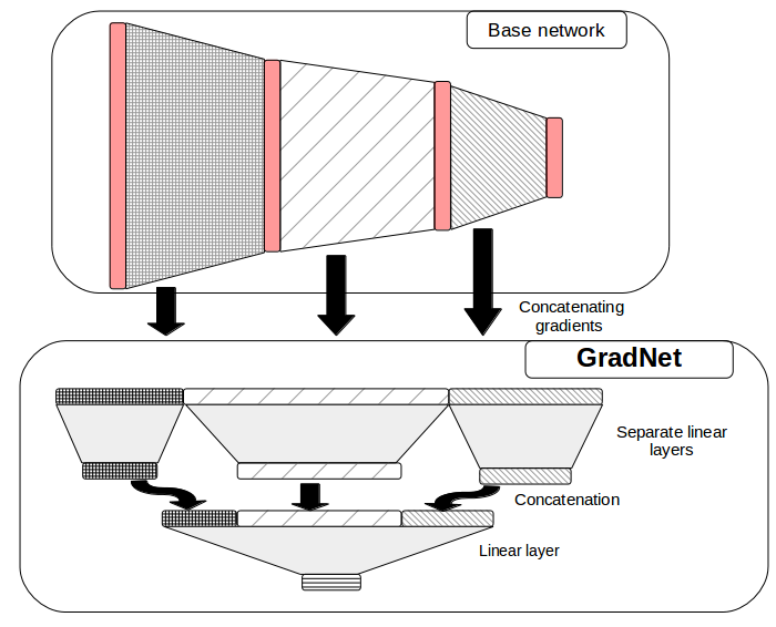
Since our models are discriminative and not generative, the loss surfaces are not known in absence of the labels. Hence we define GradNet, a multi-layer network over the tangent space, as $h_{\mbox{GradNet}}(x;l(x,\hat{c};\theta))$ (see Fig. 2) with the assumption that the final output of the network after training is $\arg\!\max_{c}\sum_{\hat{c}}h_{\mbox{GradNet}}(x;l(x;\hat{c},\theta)$.

Results in Denil et al., (2013); Denton et al., (2014); Choromanska et al., (2015) indicate high over-parametrization and redundancy in the parameter space, especially in deeper feedforward networks, therefore the outer product structure is highly blocked particularly in case of ReLU networks and sparsified gradients.

Figure 1: Important edges in the gradient graph of the MNIST network.

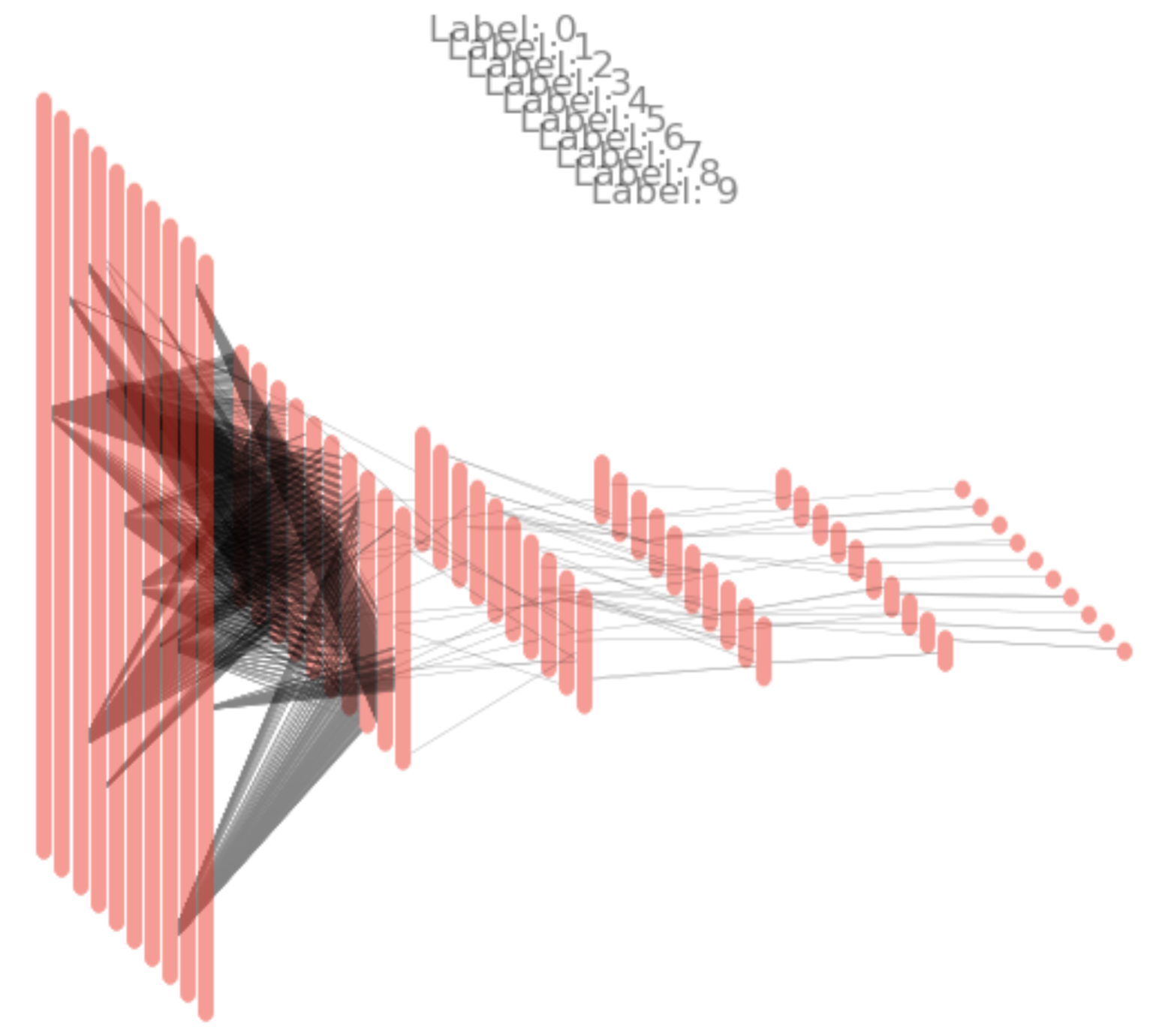
Let us consider a multi-layer perceptron with rectified linear units and a gradient graph with sparsity factor $\alpha$ corresponding to the proportion of the most important edges in the gradient graph derived by the Hessian for a particular sample. The nodes are corresponding to the parameters and we connect two nodes with a weighted edge if their value in the Hessian matrix is nonzero and their layers are neighbors. We sparsify the gradient graph layer-by-layer by the absolute weight of the edges. As shown in Fig. 1, the resulting sparse graph describes the structure of the MINST task well: for each label 0–9, a few nodes are selected in the first layer and only a few paths leave the second layer.

4 Experiments

In our first experiment we trained RBM models with $16$ and $64$ hidden units on the first half of the MNIST LeCun et al., (1998) training set and calculated the normalized gradient vectors as in ((6)). We used the RBMs output and the normalized gradient vectors within a linear model. The results in Table 1 show that the normalized gradient vector space performed very similar after some initialization with $1k$ sample and after training while the original latent space performed poorly immediately after initialization.

We assess the expressive power of the outer product manifold by inspecting the gradient-sets of several CNN’s and MLP’s. In our experiments we test the hypothesis that for a given CDFNN pre-trained for a classification problem, a quadratic separator on the gradient space can outperform the original ("base") network. We wish to find the proper separator by training a two-layer NN. In order to avoid having too much parameters to train, we chose the hidden layer of our network to have a block-like structure demonstrated in Figure 2. This model is capable of capturing connections between gradients from adjacent layers of the base network.

Figure 2: GradNet

In order to find the optimal architecture, the right normalization process and regularization technique, and the best optimization method, we experimented with a large number of setups. We measured the performance of these various kinds of GradNet models on the gradient space of a CNN trained on the first half of the CIFAR-10 Krizhevsky, (2009) training dataset. We used the other half of the dataset and random labels to generate gradient vectors to be used as training input for the GradNet. In the testing phase we use all of the gradient vectors for every data point in the test set, we give them all to the network as inputs, and we define the prediction as the index of the maximal element in the sum of the outputs.

Algorithm 1 Training procedure of GradNet

Input: Pre-trained model with parameter $\theta$, dataset $D$, GradNet $N$, normalization method $n$, number of epochs $t$

Output: Trained GradNet

1:procedure Train($M,D,N,n,t$)

2:     for epoch from 1 to t do

3:         for $batch$ in $D$ do

4:              $X\leftarrow augmentation(batch)$

5:              $c\leftarrow$ real labels for each data point in $batch$

6:              $\hat{c}\leftarrow$ random labels for each data point in $batch$

7:              $X_{g}\leftarrow\nabla_{\theta}(l(x;\hat{c},\theta))$ for each data point in the $batch$

8:              $\hat{X_{g}}\leftarrow n(X_{g})$ $\triangleright$ normalization

9:              $N\leftarrow update(N,\hat{X_{g}},c)$ $\triangleright$ update network with normalized gradients               

10:     return $N$$\triangleright$ Return trained $N$ Prediction for data point $x$: $\arg\!\max_{c}\sum_{\hat{c}}N(n(\nabla_{\theta}l(x;\hat{c},\theta)))$

During our experiments, as a starting point we stopped the underlying original CNN at $0.72$ accuraccy and compared the following settings.

• Regarding regularization, we considered using dropout, batch normalization, both of them together, or none.

• We experimented with SGD and Adam optimization methods.

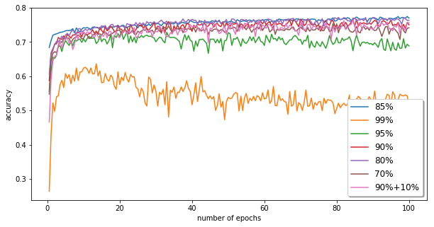
• Since we suspected that not all coordinates of the gradients are equally important, we only used the elements of large absolute value making the process computationally less expensive. We kept the elements of absolute value greater than the $q$-th percentile of the absolute value vector, and we tested our model setting this $q$ value for 99, 95, 90, 85, 80 and 70. We also tried a method where we pre-computed the indices of the most important 10$\%$ of the values for each label, and used this together with the above technique.

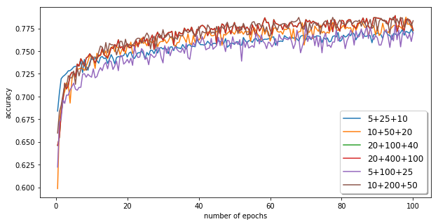
• In order to determine the exact structure of the GradNet, we tried layers and blocks of different sizes. These models differ only in the size and partition of the middle layer, which were the following in our tests: 5+25+10; 20+100+40; 10+50+20; 5+100+25; 10+200+50; 20+400+100.

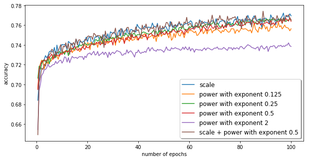
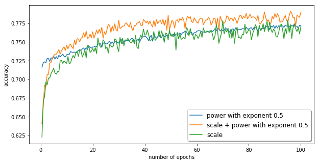
• In terms of normalization, we ran tests using standard norm with and without L2-norm following it; scale norm; power norm with exponents $\frac{1}{8}$, $\frac{1}{4}$, $\frac{1}{2}$, and $2$; and scale norm followed by power norm with exponent $\frac{1}{2}$.

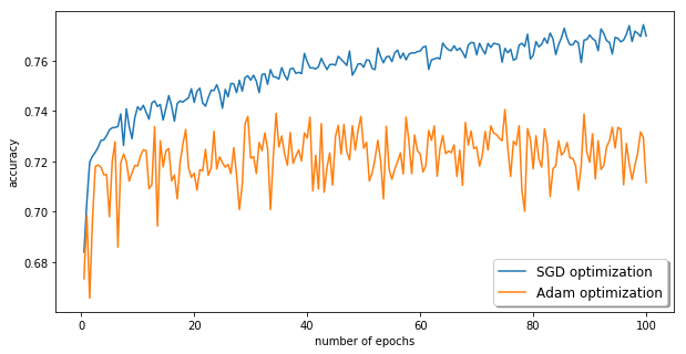
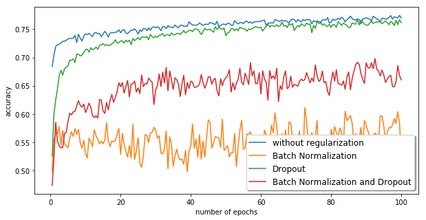
Learning curves for the different networks are presented in Figures 4 - 8. We observed that SGD gives a better performance than Adam (Fig. 4), and that regularization is not needed (Fig. 4). We also found that it is sufficient to use the elements of each gradient vector that are greater than the 85-th percentile of all of the absolute values in the vector (Fig. 6). Regarding structure, the best-performing GradNet was the one with hidden layer of size 130 partitioned into sublayers of sizes 5, 100 and 25 (Fig. 6). Interestingly, the GradNet surprassed the performance of the underlying CNN, at some settings even after only one epoch. Out of all the considered normalization methods, the scale norm and the power norm together gave the most satisfactory outcome (Fig. 8,8).

Table 1: Performance measure of the normalized gradient based on RBM.

MNIST
#hidden	Original	Improved
16	0.6834	0.9675
16	0.8997	0.9734
64	0.872	0.9822
64	0.9134	0.9876

Figure 3: Optimization methods

Figure 4: Regularization methods

Figure 5: Selection percentile

Figure 6: Structure

Figure 7: Normalization with structure 5+25+10

Figure 8: Normalization with structure 5+100+25

To show the performance of the GradNet with these particular settings, we took snapshots of a CNN at progressively increasing levels of pre-training, and we trained the GradNet on the gradient sets of these networks. We ran these tests using a CNN trained on half of the CIFAR dataset and with one trained on half of MNIST. Table 2 shows the accuracies of all the base networks together with the accuracies of the corresponding GradNets.

Table 2: Performance measure of the improved networks.

CIFAR
Original	Improved	Gain
0.79	0.8289	+4.9%
0.76	0.8201	+7.9%
0.74	0.8066	+9%
0.72	0.7936	+10.2%
0.68	0.7649	+12.5%
0.65	0.7511	+15.5%
0.62	0.7274	+17.3%
0.55	0.7016	+27.5%
0.51	0.6856	+34.4%
0.49	0.678	+38.3%

MNIST
Original	Improved	Gain
0.92	0.98	+6.5%
0.96	0.9857	+2.7%
0.9894	0.9914	+0.2%

5 Conclusions

In this paper we proposed a class of reparametrization invariant metrics for discriminative feed-forward networks based on the underlying Riemannian structure. By approximation of the inner product, we showed promising results with our GradNet network in the sparsified gradient space. GradNet outperformed the original network even if built from a few epochs of the original network. We proposed a closed approximation for Restricted Boltzmann Machines and outer product metrics. Our results show high invariance to reparametrization in RBM. In the future, we would like to extend our method to Hessian metrics and further investigate sparsity and possible transitions to less complex manifolds via pushforward and random orthogonal transformations.

References

- Amari, (1996) Amari, S.-i. (1996). Neural learning in structured parameter spaces-natural Riemannian gradient. In NIPS, pages 127–133. Citeseer.
- Amari and Armstrong, (2014) Amari, S.-i. and Armstrong, J. (2014). Curvature of Hessian manifolds. Differential Geometry and its Applications, 33:1–12.
- Bartlett and Maass, (2003) Bartlett, P. L. and Maass, W. (2003). Vapnik-Chervonenkis dimension of neural nets. The handbook of brain theory and neural networks, pages 1188–1192.
- Bengio and Delalleau, (2011) Bengio, Y. and Delalleau, O. (2011). On the expressive power of deep architectures. In International Conference on Algorithmic Learning Theory, pages 18–36. Springer.
- Bishop, (1992) Bishop, C. (1992). Exact calculation of the hessian matrix for the multilayer perceptron.
- Campbell, (1986) Campbell, L. (1986). An extended Čencov characterization of the information metric. Proceedings of the American Mathematical Society, 98(1):135–141.
- Choromanska et al., (2015) Choromanska, A., Henaff, M., Mathieu, M., Arous, G. B., and LeCun, Y. (2015). The loss surfaces of multilayer networks. In Artificial Intelligence and Statistics, pages 192–204.
- Denil et al., (2013) Denil, M., Shakibi, B., Dinh, L., De Freitas, N., et al. (2013). Predicting parameters in deep learning. In Advances in neural information processing systems, pages 2148–2156.
- Denton et al., (2014) Denton, E. L., Zaremba, W., Bruna, J., LeCun, Y., and Fergus, R. (2014). Exploiting linear structure within convolutional networks for efficient evaluation. In Advances in neural information processing systems, pages 1269–1277.
- Goodfellow et al., (2014) Goodfellow, I., Pouget-Abadie, J., Mirza, M., Xu, B., Warde-Farley, D., Ozair, S., Courville, A., and Bengio, Y. (2014). Generative adversarial nets. In Advances in neural information processing systems, pages 2672–2680.
- Greff et al., (2017) Greff, K., Srivastava, R. K., Koutník, J., Steunebrink, B. R., and Schmidhuber, J. (2017). Lstm: A search space odyssey. IEEE transactions on neural networks and learning systems.
- Hammersley and Clifford, (1971) Hammersley, J. M. and Clifford, P. (1971). Markov fields on finite graphs and lattices. seminar, unpublished.
- He et al., (2016) He, K., Zhang, X., Ren, S., and Sun, J. (2016). Deep residual learning for image recognition. In Proceedings of the IEEE Conference on Computer Vision and Pattern Recognition, pages 770–778.
- Hinton, (2002) Hinton, G. E. (2002). Training products of experts by minimizing contrastive divergence. Neural computation, 14(8):1771–1800.
- Ioffe and Szegedy, (2015) Ioffe, S. and Szegedy, C. (2015). Batch normalization: Accelerating deep network training by reducing internal covariate shift. arXiv preprint arXiv:1502.03167.
- Jaakkola et al., (1999) Jaakkola, T. S., Haussler, D., et al. (1999). Exploiting generative models in discriminative classifiers. Advances in neural information processing systems, pages 487–493.
- Kingma and Ba, (2014) Kingma, D. and Ba, J. (2014). Adam: A method for stochastic optimization. arXiv preprint arXiv:1412.6980.
- Kingma and Welling, (2013) Kingma, D. P. and Welling, M. (2013). Auto-encoding variational bayes. arXiv preprint arXiv:1312.6114.
- Kirkpatrick et al., (2017) Kirkpatrick, J., Pascanu, R., Rabinowitz, N., Veness, J., Desjardins, G., Rusu, A. A., Milan, K., Quan, J., Ramalho, T., Grabska-Barwinska, A., et al. (2017). Overcoming catastrophic forgetting in neural networks. Proceedings of the National Academy of Sciences, 114(13):3521–3526.
- Krizhevsky, (2009) Krizhevsky, A. (2009). Learning multiple layers of features from tiny images.
- Krogh and Hertz, (1992) Krogh, A. and Hertz, J. A. (1992). A simple weight decay can improve generalization. In Advances in neural information processing systems, pages 950–957.
- LeCun et al., (1998) LeCun, Y., Bottou, L., Bengio, Y., and Haffner, P. (1998). Gradient-based learning applied to document recognition. Proceedings of the IEEE, 86(11):2278–2324.
- LeCun and Cortes, (2010) LeCun, Y. and Cortes, C. (2010). MNIST handwritten digit database.
- Lin and Tegmark, (2016) Lin, H. W. and Tegmark, M. (2016). Why does deep and cheap learning work so well? arXiv preprint arXiv:1608.08225.
- Nesterov, (1983) Nesterov, Y. (1983). A method of solving a convex programming problem with convergence rate o (1/k2). In Soviet Mathematics Doklady, volume 27, pages 372–376.
- Ollivier, (2015) Ollivier, Y. (2015). Riemannian metrics for neural networks i: feedforward networks. Information and Inference: A Journal of the IMA, 4(2):108–153.
- Perronnin and Dance, (2007) Perronnin, F. and Dance, C. (2007). Fisher kernels on visual vocabularies for image categorization. In Computer Vision and Pattern Recognition, 2007. CVPR’07. IEEE Conference on, pages 1–8. IEEE.
- Ren et al., (2015) Ren, S., He, K., Girshick, R., and Sun, J. (2015). Faster r-cnn: Towards real-time object detection with region proposal networks. In Advances in neural information processing systems, pages 91–99.
- Rifai et al., (2011) Rifai, S., Dauphin, Y., Vincent, P., Bengio, Y., and Muller, X. (2011). The manifold tangent classifier. In NIPS, volume 271, page 523.
- Rolnick and Tegmark, (2017) Rolnick, D. and Tegmark, M. (2017). The power of deeper networks for expressing natural functions. arXiv preprint arXiv:1705.05502.
- Rumelhart et al., (1985) Rumelhart, D. E., Hinton, G. E., and Williams, R. J. (1985). Learning internal representations by error propagation. Technical report, DTIC Document.
- Shima, (1995) Shima, H. (1995). Hessian manifolds of constant hessian sectional curvature. Journal of the Mathematical Society of Japan, 47(4):735–753.
- Silver et al., (2017) Silver, D., Schrittwieser, J., Simonyan, K., Antonoglou, I., Huang, A., Guez, A., Hubert, T., Baker, L., Lai, M., Bolton, A., et al. (2017). Mastering the game of go without human knowledge. Nature, 550(7676):354.
- Sontag, (1998) Sontag, E. D. (1998). VC dimension of neural networks. NATO ASI Series F Computer and Systems Sciences, 168:69–96.
- Srivastava et al., (2014) Srivastava, N., Hinton, G., Krizhevsky, A., Sutskever, I., and Salakhutdinov, R. (2014). Dropout: A simple way to prevent neural networks from overfitting. The Journal of Machine Learning Research, 15(1):1929–1958.
- Szegedy et al., (2016) Szegedy, C., Vanhoucke, V., Ioffe, S., Shlens, J., and Wojna, Z. (2016). Rethinking the inception architecture for computer vision. In Proceedings of the IEEE Conference on Computer Vision and Pattern Recognition, pages 2818–2826.
- C̆encov, (1982) C̆encov, N. N. (1982). Statistical decision rules and optimal inference. American Mathematical Society, 53.
- Vinyals et al., (2017) Vinyals, O., Toshev, A., Bengio, S., and Erhan, D. (2017). Show and tell: Lessons learned from the 2015 mscoco image captioning challenge. IEEE transactions on pattern analysis and machine intelligence, 39(4):652–663.
- Zeiler, (2012) Zeiler, M. D. (2012). Adadelta: an adaptive learning rate method. arXiv preprint arXiv:1212.5701.
- (40) Zhang, C., Bengio, S., Hardt, M., Recht, B., and Vinyals, O. (2016a). Understanding deep learning requires rethinking generalization. arXiv preprint arXiv:1611.03530.
- (41) Zhang, H., Reddi, S. J., and Sra, S. (2016b). Riemannian svrg: fast stochastic optimization on riemannian manifolds. In Advances in Neural Information Processing Systems, pages 4592–4600.