Linear Model Regression on Time-series Data:
Non-asymptotic Error Bounds and Applications

Abstract

Data-driven methods for modeling dynamic systems have recently received considerable attention as they provide a mechanism for control synthesis directly from the observed time-series data. In the absence of prior assumptions on how the time-series had been generated, regression on the system model has been particularly popular. In the linear case, the resulting least squares setup for model regression, not only provides a computationally viable method to fit a model to the data, but also provides useful insights into the modal properties of the underlying dynamics. Although probabilistic estimates for this model regression have been reported, deterministic error bounds have not been examined in the literature, particularly as they pertain to the properties of the underlying system. In this paper, we provide deterministic non-asymptotic error bounds for fitting a linear model to observed time-series data, with a particular attention to the role of symmetry and eigenvalue multiplicity in the underlying system matrix.

Keywords: data-driven methods, linear regression, linear models, supervised learning

I INTRODUCTION

Recent advances in measurement and sensing technologies have lead to the availability of an unprecedented amount of data generated by complex physical, social, and biological systems such as turbulent flow, opinion dynamics on social networks, transportation, financial trading, and drug discovery. This so-called big data revolution has resulted in the development of efficient computational tools that utilizes the data generated by a dynamic system to reason about reduce order representations of this data, subsequently utilized for classification or prediction on the underlying model. Such techniques have been particularly useful when the derivation of models from first principles is prohibitively complex or infeasible. In the meantime, utilizing data generated by the system directly for the purpose of control or estimation, poses a number of challenges, most notably for model-based control design techniques such as ${\cal H}_{2}$, ${\cal H}_{\infty}$, and model predictive control (MPC). As such, it has become imperative to examine fundamental limits on fitting models to the time-series data, that can subsequently be used for model-based control synthesis.

One caveat of such an approach for a wide range of complex systems is the absence of the ability to excite the system with desired (persistent) inputs for the purpose of system identification [1]. More recently, data-driven identification has also been examined in the context of machine learning as an extension of classification or prediction, with less attention given to the ability to excite the system with persistent inputs. In this direction, non-asymptotic bounds for finite sample complexity were obtained in [2, 3, 4, 5, 6] for the linear time-invariant systems. Maximum likelihood and subspace identification methods have been employed in [7] to learn linear systems with guaranteed stability. The problem was investigated in an online learning setup to find regret bounds on the average cost of linear quadratic (LQ) systems in [8]. In the context of data-driven analysis of dynamical systems, Koopman analysis has also been used for operator-theoretic identification of nonlinear systems and their spectral properties [9, 10, 11]. One of the key elements used in the aforementioned identification methods is a linear regression step in order to fit a model to data; linear regression is in fact one of the backbone of what is known as supervised learning. In its most basic form, linear regression is used to find the system parameters by solving a least-squares minimization problem constructed on the observed time-series. Examples of such an approach can be found in [12, 5, 13].

The error analysis for fitting a linear dynamic system to data presented in this work is closely related to error estimates examined in [12] and [5] for linear quadratic synthesis. In both works, control synthesis involves an intermediate step of parameterizing the underlying system using the collected data; subsequently, probabilistic guarantees on the error between the true and the estimated models are presented. In [12], the underlying system is allowed to be excited by canonical inputs before time-series data is collected following each “episode”. The same approach has been adopted in [5], where a Gaussian noise is used to excite the system. While meaningful upper bounds on the error of the estimate are examined in these works, the presented results are probabilistic in nature, with probabilistic bounds that are directly related to the number of data points. In this work, we provide non-asymptotic error bounds for adopting a regression approach to fit a linear model to data generated by the system, evolving from initial conditions and without a control input. Furthermore, this error bound is analyzed in an online (non-asymptotic) manner as more data becomes available. It is shown that the error guarantees are closely related to the system parameters, the rank of the collected data, and not surprisingly, the initial conditions. We then focus on the case where the underlying linear model is symmetric and show that the modeling regression error depends on the spectral properties of the system.

The organization of the paper is as follows: In §II, we provide the necessary mathematical background. The problem setup is outlined in §III. §IV provides the error analysis and main results of the paper. We then examine the ramification of our results for fitting a linear model to network data in §V. The paper is concluded in §VI.

II Notation and Preliminaries

The cardinality of a set $S$ is denoted as $|S|$. A column vector with $n$ real entries is denoted as $\mathbf{v}\in\mathbb{R}^{n}$, where $\mathbf{v}_{i}$ represents its $i$th element. The matrix $M\in\mathbb{R}^{p\times q}$ contains $p$ rows and $q$ columns and $[M]_{ij}$ denotes its (real) entry at the $i$th row and $j$th column. The Moore-Penrose pseudo-inverse of a full-rank matrix $M\in\mathbb{R}^{p\times q}$ is defined as $M^{\dagger}=(M^{\top}M)^{-1}M^{\top}$ if $p>q$ and $M^{\dagger}=M^{\top}(MM^{\top})^{-1}$ otherwise; $M^{\top}$ denotes the transpose of the matrix. The range and nullspace of matrix $M$ are denoted by $\mathcal{R}(M)$ and $\mathcal{N}(M)$, respectively. The basis of the vector space $\mathcal{V}$ is referred to as $\mathcal{B}(\mathcal{V})$; the span of a set of vectors, denoted by span, is the set of all linear combinations of these vectors. The unit vector $\mathbf{e}^{i}$ is the column vector with all zero entries except $[\mathbf{e}^{i}]_{i}=1$. The column vector of all ones is denoted by 1, with dimension implicit from the context. The $n\times n$ identity matrix is defined as $I_{n}=\text{\bf Diag}(\textbf{1})$ for $\mathbf{1}\in\mathbb{R}^{n}$. The trace of $M\in\mathbb{R}^{n\times n}$ is designated as $\textit{\bf Tr}\text{(}M)=\sum_{i=1}^{n}[M]_{ii}=\sum_{i=1}^{n}\lambda_{i}$, where $\lambda_{i}$ is the $i$th eigenvalue of $M$. We write $M\succ 0$ when $M$ is positive-definite (PD) and $M\succeq 0$ if $M$ is positive-semidefinite (PSD). The spectrum of $M$ (the set of its eigenvalues) is denoted by $\mathbf{\Lambda}(M)$. The algebraic multiplicity of an eigenvalue $\lambda$ is denoted by $m(\lambda)$, defined as the multiplicity of $\lambda$ in $\mathbf{\Lambda}(M)$. An eigenvalue $\lambda$ is called simple if $m(\lambda)=1$. The singular value decomposition (SVD) of a matrix $X\in\mathbb{R}^{n\times m}$ is the factorization $X={U}\Sigma{V}^{\top}$, where the unitary matrices ${U}$ and ${V}$ consist of the left and right “singular” vectors of $X$, and $\Sigma$ is the diagonal matrix of singular values. Economic SVD is the reduced order matrix obtained by truncating the factor matrices in the SVD to the first $r$ columns of $U$ and $V$, corresponding to the $r$ non-zero singular values in $\Sigma$, where $r=\text{\bf rank}(X)$. From the SVD of a given matrix $X$, one can find its pseudo-inverse as $X^{\dagger}={V}\Sigma^{-1}{U}^{\top}$, resulting in $XX^{\dagger}={U}{U}^{\top}$; when $\Sigma$ has zero diagonals, the aforementioned inverse keeps these zeros untouched. The Euclidean norm of a vector $\mathbf{x}\in\mathbb{R}^{n}$ is defined as $\|\mathbf{x}\|_{2}=(\mathbf{x}^{\top}\mathbf{x})^{1/2}=(\sum_{i=1}^{n}x_{i}^{2})^{1/2}$. The spectral norm of matrix $X$ is defined as $\|X\|_{2}=\sup\{\|X\mathbf{u}\|_{2}:\|\mathbf{u}\|_{2}=1\}$. The Frobenius norm of a matrix $\|X\|_{F}$ is defined as $\|X\|_{F}=\sqrt{\textit{\bf Tr}(X^{\top}X)}$. Spectral and Frobenius norms satisfy the inequality $\|X\|_{2}\leq\|X\|_{F}\leq r\|X\|_{2}$, where $r=\text{\bf rank}(X)$.

III Problem Setup

For a wide range of real-world systems, the underlying complex dynamics makes deriving the corresponding models from first principles difficult if not infeasible. This can be due to a range of factors from the unpredictable nature of the environment to perturbations and uncertainties in the complex system [14, 5]. However, with the availability of sensing technologies and high performance computing, time-series data can be collected from these systems. Hence, it becomes natural to consider to what extent the observed time-series can be used to reason about the underlying dynamic model. In the case when this data has been generated by simulations (a model, albeit complex, already exists), one might still be interested to reason about the dynamics using “simple” models. The adoption of this approach involves using prior knowledge of the underlying dynamics to choose a particular basis or library, and then postulating that the dynamic system is some combination of these basis elements. This problem then reduces to a parameter optimization problem -with respect to these basis or library- for their combination that best fits the given data, with respect to a suitable norm or metric. In the absence of any prior assumption on the dynamics, however, it is often desirable to explore simple models. This paper examines non-asymptotic error bounds for doing such a linear fit, for the case when the data had been generated by a linear system; generically, it is the case that if the data is rich enough and the system does not have degeneracies, exact model is obtained after the number of data snapshots is the dimension of the system. In fact, we show that even in this most streamlined case, and even in the absence of noise or uncertainty in the collected data, understanding non-asymptotic behavior of the error requires some non-trivial analysis.

Consider the discrete linear time-invariant system described by the state equation,

$$\mathbf{x}_{t+1}=A\mathbf{x}_{t},\hskip 28.45274ptt=0,1,2,\ldots,$$ (1)

where $A\in\mathbb{R}^{n\times n}$ is the unknown system matrix, $\mathbf{x}_{t}\in\mathbb{R}^{n}$ is the state of the system at time $t$, and the system has been initialized from $\mathbf{x}_{0}$. The state snapshots collected up to (and including) time $k$ can now be grouped as,

$$X_{k}=[\mathbf{x}_{0}\quad\mathbf{x}_{1}\quad\dots\quad\mathbf{x}_{k}]\ ,\;Y_{k}=[\mathbf{x}_{1}\quad\mathbf{x}_{2}\quad\dots\quad\mathbf{x}_{k+1}].$$ (2)

This data collection approach is analogous to the first step of the so-called dynamic mode decomposition (DMD) algorithm [15], where this step is followed by the parameterization of the eigenvalues and eigenvectors of the underlying system model. Now to estimate the underlying system matrix at each $k$, we consider the the least-squares minimization, $\hat{A}_{k}=\text{argmin}_{A}\|Y_{k}-AX_{k}\|_{F},$ whose solution is of the form $\hat{A}_{k}=Y_{k}X_{k}^{\dagger}$; see Fig. 1. Note that when ${\textit{\bf rank}}(X_{k})=n$, $\hat{A}_{k}=AX_{k}X_{k}^{\dagger}=AX_{k}X_{k}^{\top}(X_{k}X_{k}^{\top})^{-1}=~{}A.$

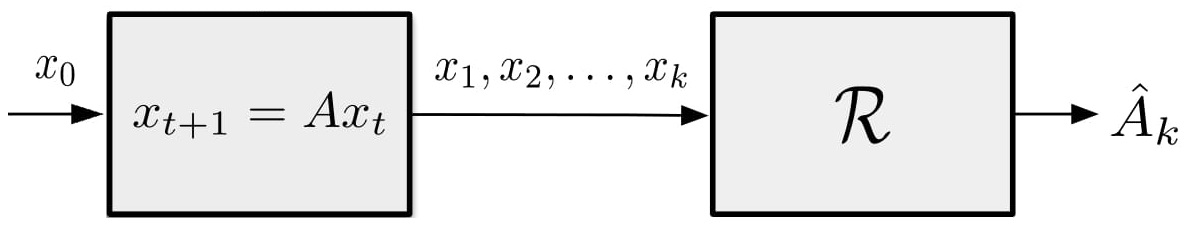
Figure 1: Estimating the underlying dynamics $A$ after $k$ data snapshots using the model regression ${\cal R}$

The focus of this paper is on the analysis of the error $\|A-\hat{A}_{k}\|$, i.e., the non-asymptotic error between the original and estimated models, using linear regression when ${\textit{\bf rank}}(X_{k})<~{}n$. Our work considers an online estimation of the model $A$, where each new data snapshot is added to the previously collected set. At any time-step $k$, an estimate for $A$ is found based on the received data up to $k$. The resulting data-driven recursive minimization is depicted in Fig. 1. Although not discussed further in this paper, we note that diagram in Fig. 1 can -in principle- be augmented with a model-based control or filtering scheme that utilizes $\hat{A}_{k}$ after a suitable number of steps. In §IV, we first introduce an upper bound on the estimation error as a function of the system dynamics $A$, the iteration count $k$, dimension of the system $n$, and the initial conditions $\mathbf{x}_{0}$. In particular, we show that for each time-step, the left-singluar vectors of the SVD of the data matrix dictate the estimation error bound. Next, we focus on symmetric system matrices. In this case, it is shown that the model regression error can be characterized by the multiplicities in the spectrum of the underlying system.

IV Non-asymptotic Error Analysis

In this section, we examine the error bound for the linear system regression in (1) based on the system characteristics and the observed data snapshots. We assume that $k<n$, i.e., the number of data snapshots is less than the size of the system. The next results, characterizes the regression estimation error as a function of the time step $k$.

Theorem 1

Consider the system in (1) and the corresponding data matrix. Let $X_{k}={U}_{k}\Sigma_{k}{V}_{k}^{\top}$ be the SVD of $X_{k}$. Then the model estimate at time-step $k$ is given by $\hat{A}_{k}=A(I-E_{k})$ where,

$$E_{k}=\left(I-\frac{S_{k}P_{k}}{\textit{\bf Tr}{(S_{k}P_{k})}}\right)S_{k}\,,$$ (3)

with,

$$S_{k}=I-{U}_{k-1}{U}_{k-1}^{\top},\quad P_{k}=\mathbf{x}_{k}\mathbf{x}_{k}^{\top}=A^{k}\mathbf{x}_{0}\mathbf{x}_{0}^{\top}A^{k^{\top}}\,.$$ (4)

Moreover,

$$\|E_{k}\|_{2}\leq\left\|I-\frac{S_{k}P_{k}}{\textit{\bf Tr}{(S_{k}P_{k})}}\right\|_{2}.$$ (5)

Proof:

From (2), $X_{k}=\begin{bmatrix}X_{k-1}&A^{k}\mathbf{x}_{0}\end{bmatrix}$, and $Y_{k}=AX_{k}=A\begin{bmatrix}X_{k-1}&A^{k}\mathbf{x}_{0}\end{bmatrix}$. Then the estimate of the system matrix after the $k$-th snapshot is given by $\hat{A}_{k}=Y_{k}X_{k}^{\dagger}$, where $\hat{A}_{k}$ is the least-squares solution to $AX_{k}=Y_{k}$. Thus,

$$\hat{A}_{k}=Y_{k}X_{k}^{\dagger}=AX_{k}X_{k}^{\dagger}=A\begin{bmatrix}X_{k-1}&A^{k}\mathbf{x}_{0}\end{bmatrix}X_{k}^{\dagger}\ .$$ (6)

Hence we need to characterize $X_{k}^{\dagger}$. To this end, we start from $X_{k}^{\dagger}=\left(X_{k}^{\top}X_{k}\right)^{-1}X_{k}^{\top}$. We first note that,

$$X_{k}^{\top}X_{k} =\begin{bmatrix}X_{k-1}^{\top}\\ \mathbf{x}_{0}^{\top}A^{k^{\top}}\end{bmatrix}\begin{bmatrix}X_{k-1}&A^{k}\mathbf{x}_{0}\end{bmatrix}$$

$$=\begin{bmatrix}X_{k-1}^{\top}X_{k-1}&X_{k-1}^{\top}A^{k}\mathbf{x}_{0}\\ \mathbf{x}_{0}^{\top}A^{k^{\top}}X_{k-1}&\mathbf{x}_{0}^{\top}A^{k^{\top}}A^{k}\mathbf{x}_{0}\end{bmatrix}\,.$$

Then

$$\left(X_{k}^{\top}X_{k}\right)^{-1}=\frac{1}{\zeta}\begin{bmatrix}\Phi&-X_{k-1}^{\dagger}A^{k}\mathbf{x}_{0}\\ -\mathbf{x}_{0}^{\top}A^{k^{\top}}X_{k-1}^{{\dagger}^{\top}}&1\end{bmatrix},$$

where

$$\Phi =\left(X_{k-1}^{\top}X_{k-1}\right)^{-1}\left[\zeta I+X_{k-1}^{\top}A^{k}\mathbf{x}_{0}\mathbf{x}_{0}^{\top}A^{k^{\top}}X_{k-1}^{{\dagger}^{\top}}\right],$$

$$\zeta =\mathbf{x}_{0}^{\top}A^{k^{\top}}\left[I-X_{k-1}\left(X_{k-1}^{\top}X_{k-1}\right)^{-1}X_{k-1}^{\top}\right]A^{k}\mathbf{x}_{0}$$

$$=-\mathbf{x}_{0}^{\top}A^{k^{\top}}\left[X_{k-1}X_{k-1}^{\dagger}-I\right]A^{k}\mathbf{x}_{0}\ .$$

In the meantime, $X_{k}^{\dagger}=\left(X_{k}^{\top}X_{k}\right)^{-1}X_{k}^{\top}\begin{bmatrix}\Psi_{1}\\ \Psi_{2}\end{bmatrix}$, with,

$$\Psi_{1} =X_{k-1}^{\dagger}+\frac{1}{\zeta}X_{k-1}^{\dagger}A^{k}\mathbf{x}_{0}\mathbf{x}_{0}^{\top}A^{k^{\top}}\left({U}_{k-1}{U}_{k-1}^{\top}-I\right),$$

$$\Psi_{2} =-\frac{1}{\zeta}\mathbf{x}_{0}^{\top}A^{k^{\top}}\left({U}_{k-1}{U}_{k-1}^{\top}-I\right),$$

where we have used the fact $X_{k-1}X_{k-1}^{\dagger}={U}_{k-1}{U}_{k-1}^{\top}$. Thereby, we can expand $\hat{A}_{k}$ from (6) as,

$$\hat{A}_{k}=AX_{k}X_{k}^{\dagger}=A\left({U}_{k-1}{U}_{k-1}^{\top}\right)$$

$$+A\left(\frac{1}{\zeta}\left({U}_{k-1}{U}_{k-1}^{\top}-I\right)A^{k}\mathbf{x}_{0}\mathbf{x}_{0}^{\top}A^{k^{\top}}\left({U}_{k-1}{U}_{k-1}^{\top}-I\right)\right)$$

$$=A\left({U}_{k-1}{U}_{k-1}^{\top}\right)$$

$$-A\left(\frac{\left({U}_{k-1}{U}_{k-1}^{\top}-I\right)A^{k}\mathbf{x}_{0}\mathbf{x}_{0}^{\top}A^{k^{\top}}\left({U}_{k-1}\mathcal{U}_{k-1}^{\top}-I\right)}{\mathbf{x}_{0}^{\top}A^{k^{\top}}\left({U}_{k-1}{U}_{k-1}^{\top}-I\right)A^{k}\mathbf{x}_{0}}\right)\,,$$

and from (4), the estimated model $\hat{A}_{k}$ at time-step $k$ is given by $\hat{A}_{k}=A\left(I-E_{k}\right)$ with,

$$E_{k} =\frac{\Big{(}\textit{\bf Tr}{(S_{k}P_{k})}I-S_{k}P_{k}\Big{)}S_{k}}{\textit{\bf Tr}{(S_{k}P_{k})}}=\left(I-\frac{S_{k}P_{k}}{\textit{\bf Tr}{(S_{k}P_{k})}}\right)S_{k}.$$

The magnitude of this error simplifies for the case of the spectral norm as,

$$\|E_{k}\|_{2}=\left\|\left(I-\frac{S_{k}P_{k}}{\textit{\bf Tr}{(S_{k}P_{k})}}\right)S_{k}\right\|_{2}\leq\left\|I-\frac{S_{k}P_{k}}{\textit{\bf Tr}{(S_{k}P_{k})}}\right\|_{2},$$

since $\|S_{k}\|_{2}=1$ for $k<n$. Lastly, we note that $S_{k}$ is the projection onto the null space of $X_{k-1}$ and $P_{k}$ is the covariance matrix of the data at time-step $k$; as such both matrices are positive-semidefinite. ∎

We note that the relation (3) captures -in a succinct way- the dependency of the model regression error on how new modes are revealed by the data stream over time.

IV-A Non-asymptotic Error Analysis for Symmetric Systems

In this section, we consider linear systems with symmetric dynamics with the aim of characterizing fundamental bounds on the regression error in terms of the spectral properties of the system. This insight into the regression error is achieved through the spectral decomposition of the system matrix,

$$A=Q\Lambda Q^{\top}=\sum_{i=1}^{r}\lambda_{i}\mathbf{q}_{i}\mathbf{q}_{i}^{\top},$$ (7)

where $Q$ is the unitary matrix containing the eigenvectors corresponding to nonzero eigenvalues of $A$, $\Lambda$ is the diagonal matrix of nonzero eigenvalues, and $r=\textbf{rank}(A)$. Symmetric system matrices appear in a wide range of applications where interactions leading to the dynamics is bidirectional; such systems are of interest in biological networks [16], social interactions [17], robotic swarms [18], and networks security [19]. Using this spectral decomposition of symmetric systems, we show that the regression error is dependent on the multiplicity of eigenvalues in $A$. In particular, we show that if $m(\lambda)=1,\forall\lambda\in\mathbf{\Lambda}(A)$, then the upper bound (5) is a function of the largest and smallest singular values of the system matrix as well as its rank. Otherwise, the regression error is $\max_{i:m(\lambda_{i})>1}|\lambda_{i}|$. We provide the details of the approach for each case.

IV-A1 Simple Eigenvalues

We first consider the case when the symmetric system matrix has simple eigenvalues and rank $r$. In reference to (7), consider the entire set of eigenvectors of $A$ consisting of $Q=[\mathbf{q}_{1}\ \cdots\ \mathbf{q}_{r}]$ and $\bar{Q}=[\bar{\mathbf{q}}_{r+1}\ \cdots\ \bar{\mathbf{q}}_{n}]$, where $\{\mathbf{q}_{1},\cdots,\mathbf{q}_{r},\bar{\mathbf{q}}_{r+1},\cdots,\bar{\mathbf{q}}_{n}\}$ forms a basis for the entire $\mathbb{R}^{n}$. Then the nonzero random initial state $\mathbf{x}_{0}$ can be written as,

$$\mathbf{x}_{0}=Q\nu+\bar{Q}\mu=\sum_{i=1}^{r}\nu_{i}\mathbf{q}_{i}+\sum_{i=r+1}^{n}\mu_{i}\bar{\mathbf{q}}_{i}\quad\quad\mathbf{\nu}\neq 0.$$ (8)

Lemma 1

For the symmetric linear system decomposed as (7), we have, $A-\hat{A}_{k}=A\Big{(}I-\frac{S_{k}Q\Lambda^{k}\nu\nu^{\top}\Lambda^{k}Q^{\top}}{\|S_{k}Q\Lambda^{k}\nu\|^{2}}\Big{)}S_{k}$.

Proof:

From (8) and (4) we have, $P_{k}=A^{k}\mathbf{x}_{0}\mathbf{x}_{0}^{\top}A^{k^{\top}}$

$$=(Q\Lambda^{k}Q^{\top})(Q\nu+\bar{Q}\mu)(Q\nu+\bar{Q}\mu)^{\top}(Q\Lambda^{k}Q^{\top})$$

$$=Q\Lambda^{k}\nu\nu^{\top}\Lambda^{k}Q^{\top},$$

and, $\textit{\bf Tr}(S_{k}P_{k})=\textit{\bf Tr}(S_{k}Q\Lambda^{k}\nu\nu^{\top}\Lambda^{k}Q^{\top})=\|S_{k}Q\Lambda^{k}\nu\|^{2}$, where we have used that $S_{k}$ is a symmetric projection. Substituting these in (3) completes the proof. ∎

We now show that when $k<n$, the error depends on the largest and smallest eigenvalues of $A$.

Theorem 2

Consider the linear dynamical system with symmetric system matrix $A$ as in (7) and the initial state $x_{0}$ as in (8). If $k<n$, then

$$\|A-\hat{A}_{k}\|_{F}^{2}\leq\Big{(}n-\min\{k,|\nu|+\min\{|\mu|,1\}\}\Big{)}\lambda_{1}^{2}-\lambda_{n}^{2}\,,$$

where $\lambda_{n}=\lambda_{\min}(A),$ $\lambda_{1}=\lambda_{\max}(A),$ and $|\nu|$ and $|\mu|$ are the number of nonzero $\nu_{i}$’s and $\mu_{i}$’s, respectively.

Proof:

From Lemma 1 we observe that,

$$\|A-\hat{A}_{k}\|_{F}^{2}=\textit{\bf Tr}\Big{(}(A-\hat{A}_{k})^{\top}(A-\hat{A}_{k})\Big{)}$$

$$=\textit{\bf Tr}(\Lambda^{2}Q^{\top}S_{k}Q)-\frac{\nu^{\top}\Lambda^{k}Q^{\top}S_{k}Q\Lambda^{2}Q^{\top}S_{k}Q\Lambda^{k}\nu}{\nu^{\top}\Lambda^{k}Q^{\top}S_{k}Q\Lambda^{k}\nu}$$

$$=\|AS_{k}\|^{2}-\frac{\|AS_{k}Q\Lambda^{k}\nu\|^{2}}{\|S_{k}Q\Lambda^{k}\nu\|^{2}}\,.$$

In the meantime,

$$\|AS_{k}\|_{F}^{2} \leq\text{\bf rank}(S_{k})\|AS_{k}\|^{2}_{2}$$

$$\leq\text{\bf rank}(S_{k})\|A\|_{2}^{2}\|S_{k}\|_{2}^{2}=\text{\bf rank}(S_{k})\lambda_{1}^{2}(A);$$

moreover, since $\lambda_{n}(A)=\inf\limits_{y\neq 0}{\|Ay\|_{2}}/{\|y\|_{2}}$, we have

$$\frac{\|AS_{k}Q\Lambda^{k}\nu\|^{2}}{\|S_{k}Q\Lambda^{k}\nu\|^{2}}\geq\lambda_{n}^{2}(A).$$

Since $A\mathbf{q}_{i}=\lambda_{i}\mathbf{q}_{i}$ and $A\bar{\mathbf{q}}_{i}=0$, we have,

$$X_{k-1}=[\mathbf{x}_{0}\quad\mathbf{x}_{1}\quad\cdots\quad\mathbf{x}_{k-1}]$$

$$=\begin{bmatrix}\sum\limits_{i=1}^{r}\nu_{i}\mathbf{q}_{i}+\sum\limits_{i=r+1}^{n}\mu_{i}\bar{\mathbf{q}}_{i}&\sum\limits_{i=1}^{r}\lambda_{i}\nu_{i}\mathbf{q}_{i}&\cdots&\sum\limits_{i=1}^{r}\lambda_{i}^{k-1}\nu_{i}\mathbf{q}_{i}\end{bmatrix}\,.$$

Thus,

$$\text{\bf rank}(X_{k-1})=\min\{k,|\nu|+\min\{|\mu|,1\}\}\,,$$ (9)

and,

$$\text{\bf rank}(S_{k})=n-\text{\bf rank}(X_{k-1})=n-\min\{k,|\nu|+\min\{|\mu|,1\}\}\,.$$

Hence,

$$\|A-\hat{A}_{k}\|_{F}^{2}\leq\Big{(}n-\min\{k,|\nu|+\min\{|\mu|,1\}\}\Big{)}\lambda_{1}^{2}-\lambda_{n}^{2},$$

which completes the proof. ∎

IV-B Effect of Eigenvalues Multiplicity on the Regression Error

In this section, we consider the symmetric systems whose eigenvalues are not necessary simple. We will see that for such systems, the regression error $\|E_{k}\|$ converges to the largest eigenvalue with multiplicity greater than one, i.e., $\|E_{k}\|=\max_{i:m(\lambda_{i})>1}|\lambda_{i}|$ for $k\geq n$.

In order to show this, we will pursue the convention adopted in (2), (7), and (8). As in § IV-A, let $r=\text{rank}(A)$ and define $\tilde{Q}=[Q\ |\ \bar{Q}]=[\mathbf{q}_{1}\ \dots\ \mathbf{q}_{r}\ \ \bar{\mathbf{q}}_{r+1}\ \dots\ \bar{\mathbf{q}}_{n}]$, where the columns of $\tilde{Q}$ span the entire $\mathbb{R}^{n}$. Furthermore, let $\alpha=[\nu^{\top}\ \mu^{\top}]^{\top}$, where $\alpha$ and $\mu$ are from (8). The data matrix can now be re-written as,

$$X_{k} =[\mathbf{x}_{0}\quad A\mathbf{x}_{0}\quad A^{2}\mathbf{x}_{0}\quad\dots\quad A^{k}\mathbf{x}_{0}]$$ (10)

$$=\tilde{Q}\ [\tilde{Q}^{\top}\mathbf{x}_{0}\quad\Lambda\tilde{Q}^{\top}\mathbf{x}_{0}\quad\dots\quad\Lambda^{k}\tilde{Q}^{\top}\mathbf{x}_{0}].$$

From (8) and the fact that the columns of $\tilde{Q}$ are orthonormal, we have $\tilde{Q}^{\top}\mathbf{x}_{0}=[\alpha_{1}\ \alpha_{2}\ \dots\ \alpha_{n}]^{\top}$ and $\Lambda^{j}\tilde{Q}^{\top}\mathbf{x}_{0}=[\alpha_{1}\lambda_{1}^{j}\quad\alpha_{2}\lambda_{2}^{j}\quad\dots\quad\alpha_{n}\lambda_{n}^{j}]^{\top}$. Moreover, in light of (10) we can decompose the data matrix into $X_{k}=\tilde{Q}\Gamma V$ where,

$$\Gamma=\begin{bmatrix}\alpha_{1}&0&\dots&0\\ 0&\alpha_{2}&\dots&0\\ \vdots&\vdots&\ddots&\vdots\\ 0&0&\dots&\alpha_{n}\end{bmatrix},\quad V=\begin{bmatrix}1&\lambda_{1}&\dots&\lambda_{1}^{k}\\ 1&\lambda_{2}&\dots&\lambda_{2}^{k}\\ \vdots&\vdots&\ddots&\vdots\\ 1&\lambda_{n}&\dots&\lambda_{n}^{k}\end{bmatrix}.$$ (11)

The matrix $[V]_{ij}=\lambda_{i}^{j-1}$ is the Vandermonde matrix formed by the eigenvalues of $A$ and $\Gamma=\text{\bf Diag}([\alpha_{i}]_{i=1}^{n})$. Assume now that the system matrix $A$ contains $s$ distinct eigenvalues and let $\mathbf{\Lambda}^{*}(A)=\{\lambda_{t_{1}},\lambda_{t_{2}},\dots,\lambda_{t_{s}}\}$ be the set of these eigenvalues; as such, the other $n-s$ eigenvalues are repetitions of the elements in $\mathbf{\Lambda}^{*}(A)$.

For our subsequent error analysis, we will use the rank of $X_{k}$ at each time-step. The next result characterizes the rank of $X_{k}$ based on the number of the collected data.

Lemma 2

Given $k<s$, the $s\times k$ Vandermonde matrix defined by $[V_{s}]_{ij}=\lambda_{i}^{j-1},\ i\in\{1,\dots,s\},\ j\in\{1,\dots,k\}$, formed by the elements of $\mathbf{\Lambda}^{*}(A)$, has full-rank.

Proof:

Let $v_{i}$ be the $i$th column of $V_{s}$ and assume that $c_{1}v_{1}+c_{2}v_{2}+\dots+c_{k}v_{k}=0$. Consider row $p$ of the equation $c_{1}+c_{2}\lambda_{p}+\dots+c_{k}\lambda_{p}^{k}=0$. Since $\lambda_{i}\neq\lambda_{j}$ for $i\neq j$, there exist $s$ solutions to the $k$-degree polynomial,

$$P(x)=c_{0}+c_{1}x+\dots+c_{k}x^{k}=0.$$

Hence $c_{1}=c_{2}=\dots=c_{k}=0$ and $v_{i}$’s are linearly independent and since $k<s$, $V_{s}$ has full-rank. ∎

Theorem 3

Let $k$ be the number of collected data snapshots and $s=|\mathbf{\Lambda}^{*}(A)|$. Then $\text{\bf rank}(X_{k})=k$ when $k<s$ and $\text{\bf rank}(X_{k})=s$ when $k\geq s$.

Proof:

For $k<s$, it is straightforward to show that from Lemma 2, $\text{\bf rank}(X_{k})=\text{\bf rank}(V)=\text{\bf rank}(V_{s})=k$. For $k\geq s$, we know that $\text{\bf rank}(V)=\text{\bf rank}(V_{s})$, where $[V_{s}]_{ij}=\lambda_{i}^{j-1},\ i\in\{1,\dots,s\},\ j\in\{1,\dots,k+1\}$. Since $V_{s}$ has full-rank (this can be shown using the nonzero sub-matrix determinants for the first $s\times s$ block), we get $\text{\bf rank}(X_{k})=\text{\bf rank}(V)=\text{\bf rank}(V_{s})=s$. ∎

Let $k\geq s$ and $X_{k}={U}\Sigma V^{\top}$ be the SVD of $X_{k}$ where,

$$X_{k}=[{U}_{1}\quad{U}_{2}]\begin{bmatrix}\Sigma_{1}&\mathbf{0}_{s\times(k-s)}\\ \mathbf{0}_{(n-s)\times s}&\mathbf{0}_{(n-s)\times(k-s)}\end{bmatrix}\begin{bmatrix}{V}_{1}&{V}_{2}\end{bmatrix}^{\top},$$ (12)

with ${U}_{1}\in\mathbb{R}^{n\times s},\ {U}_{2}\in\mathbb{R}^{n\times(n-s)},\ \Sigma_{1}\in\mathbb{R}^{s\times s},\ {V}_{1}\in\mathbb{R}^{k\times s},\ {V}_{2}\in\mathbb{R}^{k\times(k-s)}$. The existence of ${U}_{2}$ and ${V}_{2}$ is due to the fact that $X_{k}$ is degenerate. Without loss of generality, we re-arrange the columns of $\tilde{Q}$ and $\Lambda$ such that,

$$\Lambda_{R}=\left[\begin{array}[]{c|c}\Lambda_{1}&\mathbf{0}\\ \hline\cr\mathbf{0}&\Lambda_{2}\end{array}\right]\quad,\quad\tilde{Q}_{R}=\left[\begin{array}[]{c|c}\tilde{Q}_{1}&\tilde{Q}_{2}\end{array}\right],$$ (16)

where $\Lambda_{1}=\text{\bf Diag}([\lambda_{t_{1}}\quad\lambda_{t_{2}}\quad\dots\quad\lambda_{t_{s}}])$ contains the element of $\mathbf{\Lambda}^{*}(A)$ with the corresponding eigenvectors in $\tilde{Q}_{1}\in\mathbb{R}^{n\times s}$. The remaining eigenvalues and the corresponding eigenvectors are stacked in $\Lambda_{2}\in\mathbb{R}^{(n-s)\times(n-s)}$ and $\tilde{Q}_{2}\in\mathbb{R}^{n\times(n-s)}$, respectively.

A crucial term in our analysis is ${U}_{2}^{\top}\tilde{Q}_{R}\in\mathbb{R}^{(n-s)\times n}$. This matrix multiplication combines a submatrix of ${U}$ corresponding to the repeated eigenvalues, with the orthonormal eigenvectors of the system. In the next result, we show that this term has a specific row structure.

Lemma 3

Given the convention in (16), we have ${U}_{2}^{\top}\tilde{Q}_{1}=0$, i.e., ${U}_{2}^{\top}\tilde{Q}_{R}={U}_{2}^{\top}\big{[}\tilde{Q}_{1}\mid\tilde{Q}_{2}\big{]}=\big{[}\ \mathbf{0}_{(n-s)\times s}\mid{U}_{2}^{\top}\tilde{Q}_{2}\ \big{]}$.

Proof:

From (12) we have ${U}_{2}^{\top}X_{k}=0$. Then,

$${U}_{2}^{\top}X_{k} ={U}_{2}^{\top}\tilde{Q}\tilde{Q}^{\top}X_{k}={U}_{2}^{\top}\tilde{Q}\tilde{Q}^{\top}[x_{0}\quad Ax_{0}\quad\dots\quad A^{k}x_{0}]$$

$$={U}_{2}^{\top}\tilde{Q}\big{[}\tilde{Q}^{\top}x_{0}\quad\Lambda\tilde{Q}^{\top}x_{0}\quad\dots\quad\Lambda^{k}\tilde{Q}^{\top}x_{0}\big{]}$$

$$={U}_{2}^{\top}\tilde{Q}\Gamma V=0,$$

with $\Gamma$ and $V$ defined as in (11). Define $B={U}_{2}^{\top}\tilde{Q}$ and let $\mathbf{b}_{i}=[\mathbf{b}_{i_{1}}\quad\mathbf{b}_{i_{2}}\quad\dots\quad\mathbf{b}_{i_{n}}]$ and $\mathbf{v}_{i}=[1\quad\lambda_{i}\quad\dots\quad\lambda_{i}^{k}]$ be the $i$’th rows of $B$ and $V$, respectively. Then for all $i\in\{1,2,\dots,n-s\}$ we have $B\Gamma V=0$ implying that $\mathbf{b}_{i}\Gamma V=0$; as such, $\sum_{j=1}^{n}\mathbf{b}_{i_{j}}\alpha_{j}\mathbf{v}_{j}=0$ implies that $\sum_{t=1}^{s}\mathbf{c}_{t}\mathbf{v}_{t}^{*}=0$, where $\mathbf{v}_{t}^{*}$’s are the rows of $V$ corresponding to $s$ distinct eigenvalues and $\mathbf{c}_{t}$’s are some combinations of $\mathbf{b}_{i_{j}}\alpha_{j}$’s. Since the vectors $\mathbf{v}_{t}^{*}$’s are linearly independent, we get $\mathbf{c}_{i}=0$ for all $i=1,2,\dots,s$. Considering that $\mathbf{c}_{i}=\mathbf{b}_{i_{j}}$ for the elements with simple eigenvalues, the result implies that for any row $\mathbf{v}_{j}$ corresponding to a simple eigenvalue $\lambda_{j}$ the corresponding coefficient $\mathbf{b}_{i_{j}}=0$. Hence, the structure $\big{[}\ \textbf{0}_{(n-s)\times s}\mid{U}_{2}^{\top}\tilde{Q}_{2}\ \big{]}$ follows, implying that ${U}_{2}^{\top}\tilde{Q}_{1}=0$. ∎

Definition 1

Define ${U}_{2}^{\prime}$ by permuting the columns of ${U}_{2}$ such that we obtain block diagonal matrix ${U}_{2}^{\prime\top}\tilde{Q}_{2}=\text{\bf Diag}([P_{1},P_{2},\dots,P_{\ell}])$, where $\ell$ is the number of eigenvalues $\lambda$ with $m(\lambda)>1$ and $P_{i}={U}_{2}^{{}^{\prime}i^{\top}}\tilde{Q}_{2}^{i}\in\mathbb{R}^{(m(\lambda_{i})-1)\times m(\lambda_{i})}$; as such ${U}_{2}^{{}^{\prime}i}\in\mathbb{R}^{n\times(m(\lambda_{i})-1)}$ is the matrix containing vectors in ${U}_{2}^{\prime}$ corresponding to $\lambda_{i}$ and $\tilde{Q}_{2}^{i}\in\mathbb{R}^{n\times m(\lambda_{i})}$ is the matrix of eigenvectors corresponding to $\lambda_{i}$.

Remark 1

To justify the existence of such a matrix ${U}_{2}^{\prime}$, notice that the SVD factorization in terms of ${U}$ and ${V}$ are not unique and for any such factorization, ${U}_{1}\perp{U}_{2}$.

We are now well positioned to prove the main theorem of this section.

Theorem 4

Consider the dynamics represented by (1) and (2). Let $s=|\mathbf{\Lambda}^{*}(A)|$ be the number of distinct eigenvalues of $A$. Assume that $k\geq s$ and let $\lambda^{*}=\max_{i:m(\lambda_{i})>1}|\lambda_{i}|$ be the largest eigenvalue of $A$ with multiplicity greater than one. Then $\|E_{k}\|_{2}=\|A-\hat{A}_{k}\|_{2}=\lambda^{*}$.

Proof:

We will show that $\mathbf{\Lambda}(E_{k})=\mathbf{\Lambda}(A)\backslash\mathbf{\Lambda}^{*}(A)$. The error can then be re-written as,

$$\| E_{k}\|_{2}$$

$$=\|A-\hat{A}_{k}\|_{2}=\|A-AX_{k}X_{k}^{\dagger}\|_{2}=\|A(I-X_{k}X_{k}^{\dagger})\|_{2}$$

$$=\left\|A\Big{(}I-{U}_{1}\Sigma_{1}{V}_{1}^{\top}{V}_{1}\Sigma_{1}^{-1}{U}_{1}^{\top}\Big{)}\right\|_{2}=\|A(I-{U}_{1}{U}_{1}^{\top})\|_{2}$$

$$=\|A{U}_{2}^{\prime}{U}_{2}^{\prime\top}\|_{2}=\|\tilde{Q}\Lambda\tilde{Q}^{\top}{U}_{2}^{\prime}{U}_{2}^{\prime\top}\|_{2}=\|\Lambda\tilde{Q}^{\top}U_{2}^{\prime}{U}_{2}^{\prime\top}\tilde{Q}\|_{2}$$

$$=\|\Lambda({U}_{2}^{\prime\top}\tilde{Q})^{\top}({U}_{2}^{\prime\top}\tilde{Q})\|_{2},$$

where ${U}_{2}^{\prime}$ pertains to definition 1 and $I-{U}_{1}{U}_{1}^{\top}={U}_{2}^{\prime}{U}_{2}^{\prime\top}$ is the projection matrix onto ${\cal N}(X_{k}^{\top})$. Note that since the columns of ${U}_{2}^{\prime}$ are linearly independent, we have $\text{\bf rank}(E_{k})=\text{\bf rank}(A{U}_{2}^{\prime}{U}_{2}^{\prime\top})=n-s$. From Lemma 3,

$$\Lambda({U}_{2}^{\prime\top}\tilde{Q})^{\top}({U}_{2}^{\prime\top}\tilde{Q})=\Lambda\begin{bmatrix}\mathbf{0}\\ ({U}_{2}^{\prime\top}\tilde{Q}_{2})^{\top}\end{bmatrix}\begin{bmatrix}\mathbf{0}&{U}_{2}^{\prime\top}\tilde{Q}_{2}\end{bmatrix}$$ (17)

$$=\left[\begin{array}[]{c|c}\mathbf{0}_{s\times s}&\mathbf{0}_{s\times(n-s)}\\ \hline\cr\mathbf{0}_{(n-s)\times s}&\Lambda_{2}({U}_{2}^{\prime\top}\tilde{Q}_{2})^{\top}({U}_{2}^{\prime\top}\tilde{Q}_{2})\end{array}\right].$$

Then from definition 1, $\Lambda_{2}({U}_{2}^{\prime\top}\tilde{Q}_{2})^{\top}({U}_{2}^{\prime\top}\tilde{Q}_{2})=\text{\bf Diag}([\lambda_{1}P_{1}^{\top}P_{1}\ ,\ \lambda_{2}P_{2}^{\top}P_{2}\ ,\ \dots\ ,\ \lambda_{\ell}P_{\ell}^{\top}P_{\ell}])$. Consider the $i$th block $\lambda_{i}P_{i}^{\top}P_{i}$. Notice that from definition $\text{\bf rank}(P_{i}^{\top}P_{i})=m(\lambda_{i})-1$, and since ${U}_{2}^{{}^{\prime}i^{\top}}$ and $\tilde{Q}_{2}^{i}$ are orthonormal, $\lambda_{i}P_{i}^{\top}P_{i}=\lambda_{i}\tilde{Q}_{2}^{i^{\top}}{U}_{2}^{{}^{\prime}i}{U}_{2}^{{}^{\prime}i^{\top}}\tilde{Q}_{2}^{i}$ has the spectrum $\mathbf{\Lambda}(\lambda_{i}P_{i}^{\top}P_{i})=\{0,\lambda_{i},\dots,\lambda_{i}\}$. Then having $\ell$ of these blocks $\mathbf{\Lambda}(E_{k})=\mathbf{\Lambda}(A)\backslash\mathbf{\Lambda}^{*}(A)$, i.e., the spectrum of $E_{k}$ contains all repeated eigenvalues of $A$.

Since both $\Lambda$ and $({U}_{2}^{\prime\top}\tilde{Q})^{\top}({U}_{2}^{\prime\top}\tilde{Q})$ are symmetric square block diagonal matrices, the product $\Lambda({U}_{2}^{\prime\top}\tilde{Q})^{\top}({U}_{2}^{\prime\top}\tilde{Q})$ is symmetric and therefore $\|E_{k}\|_{2}=\|\Lambda({U}_{2}^{\prime\top}\tilde{Q})^{\top}({U}_{2}^{\prime\top}\tilde{Q})\|_{2}=\max\limits_{i=1,\dots,\ell}\lambda_{i}=\lambda^{*}$. ∎

V Model Regression on Networks

We now provide an example to demonstrate the applicability of the error bounds on networked systems. Consider the Petersen graph on 10 nodes and 15 edges as shown in Fig. 2. We use the weighted version of this specific structure to find error bounds on a system with simple eigenvalues. The dynamics of this system is defined using the graph Laplacian, defined as $\mathcal{L}=D-A$, where $A$ is the adjacency matrix that defines the connections in the network and $D$ is the degree matrix defined as $D_{ii}=\sum_{j}|W_{ij}|$; in this case $W_{ij}$ is the weight of the edge between nodes $i$ and $j$. Network symmetries typically induce eigenvalue multiplicities in the corresponding adjacency and Laplacian matrices. Hence to make the system more generic, we add weights $w_{1,6}=1$, $w_{2,7}=2$, $w_{3,8}=3$, $w_{4,9}=4$, and $w_{5,10}=5$ and for all other weights we have $w_{i,j}=1$. For each component $i$ the dynamics depend on the adjacent nodes in the graph $\dot{x}_{i}=\sum_{j}|W_{ij}|(x_{i}-x_{j})$. Then the overall dynamics can be written as $\dot{x}=-\mathcal{L}x$. The model regression algorithm discussed in this paper leads to the error shown in Fig. 2. For this simulation, the initial condition has been chosen as a (normalized) random vector $x_{0}\in\mathbb{R}^{10}$. The upper subfigure shows the comparison of the bound for general case using the spectral norm and the lower subfigure demonstrates the same setup for IV-A. It can be seen that the error converges to zero after $k=10$ steps, since the system matrix has simple eigenvalues.

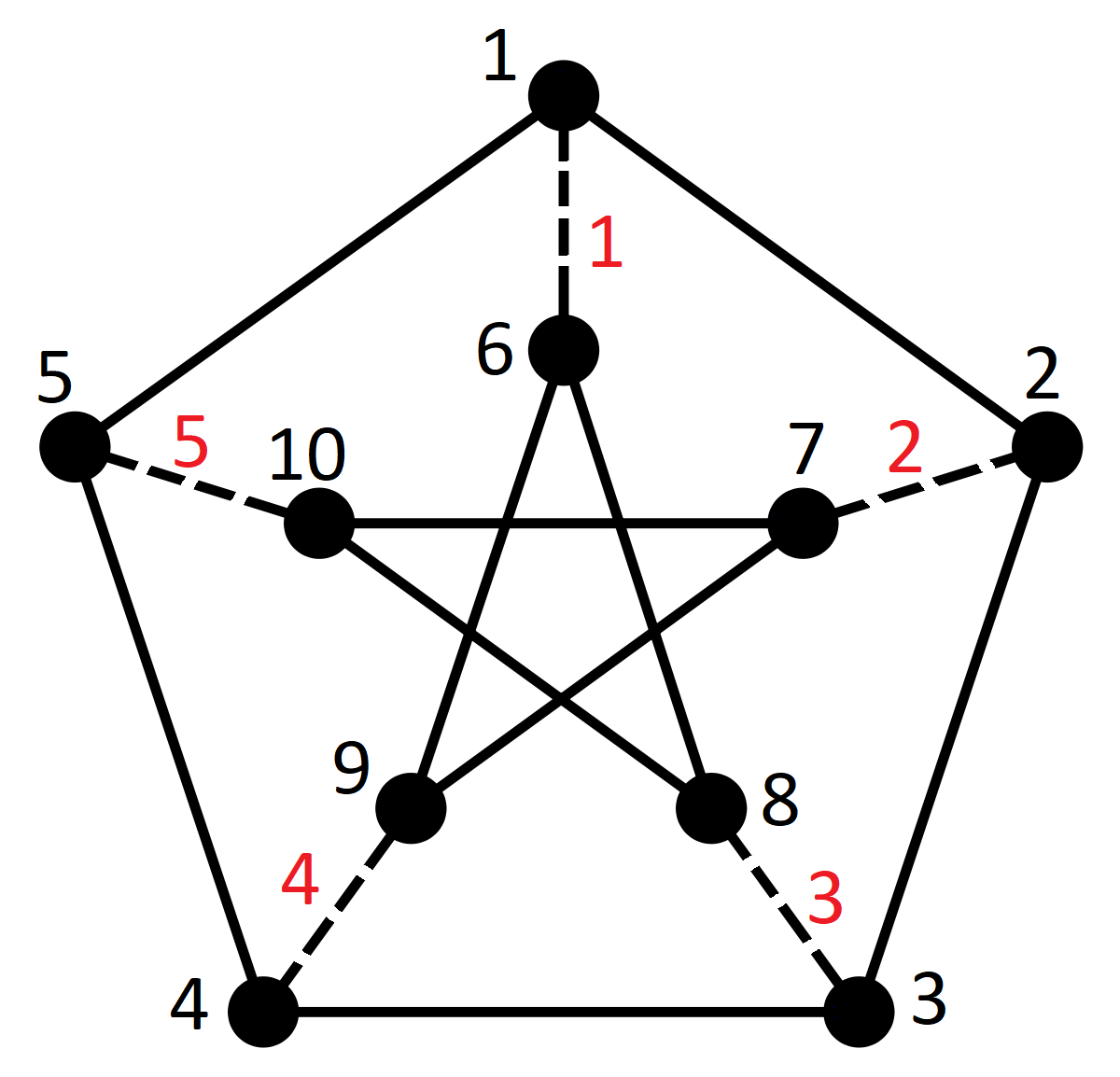
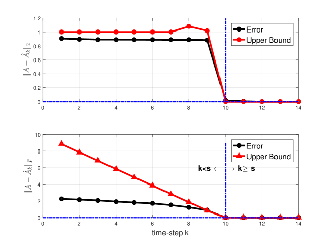
Figure 2: (left) weighted Petersen graph; (right): model regression error the corresponding theoretical error bound

VI CONCLUSION

In this paper we consider the regression approach for learning linear time-invariant dynamic models from time-series data. In particular, we showed how the richness in the data as well as spectral properties of the model, dictate fundamental bounds on the error obtained from the streaming model regression. Our subsequent works will utilize these insights to provide an active learning mechanism that has the dual role of reducing the regression error in addition to achieving auxiliary control objectives.

References

- [1] L. Ljung, “System identification,” in Signal analysis and prediction, pp. 163–173, Springer, 1998.
- [2] M. Hardt, T. Ma, and B. Recht, “Gradient descent learns linear dynamical systems,” arXiv preprint arXiv:1609.05191, 2016.
- [3] M. C. Campi and E. Weyer, “Finite sample properties of system identification methods,” IEEE Transactions on Automatic Control, vol. 47, no. 8, pp. 1329–1334, 2002.
- [4] S. Oymak and N. Ozay, “Non-asymptotic identification of lti systems from a single trajectory,” arXiv preprint arXiv:1806.05722, 2018.
- [5] S. Dean, H. Mania, N. Matni, B. Recht, and S. Tu, “On the sample complexity of the linear quadratic regulator,” arXiv preprint arXiv:1710.01688, 2017.
- [6] M. Simchowitz, H. Mania, S. Tu, M. I. Jordan, and B. Recht, “Learning without mixing: Towards a sharp analysis of linear system identification,” arXiv preprint arXiv:1802.08334, 2018.
- [7] B. Boots, “Learning stable linear dynamical systems,” Online]. Avail.: https://www. ml. cmu. edu/research/dap-papers/dap_boots. pdf, 2009.
- [8] Y. Abbasi-Yadkori and C. Szepesvári, “Regret bounds for the adaptive control of linear quadratic systems,” in Proceedings of the 24th Annual Conference on Learning Theory, pp. 1–26, 2011.
- [9] A. Mauroy and J. Goncalves, “Linear identification of nonlinear systems: A lifting technique based on the koopman operator,” in 55th Conference on Decision and Control, pp. 6500–6505, IEEE, 2016.
- [10] M. H. de Badyn, S. Alemzadeh, and M. Mesbahi, “Controllability and data-driven identification of bipartite consensus on nonlinear signed networks,” in 56th Conference on Decision and Control, pp. 3557–3562, IEEE, 2017.
- [11] S. L. Brunton, B. W. Brunton, J. L. Proctor, and J. N. Kutz, “Koopman invariant subspaces and finite linear representations of nonlinear dynamical systems for control,” PloS one, vol. 11, no. 2.
- [12] C.-N. Fiechter, “PAC adaptive control of linear systems,” in Conference on Computational learning theory, pp. 72–80, ACM, 1997.
- [13] B. Parsa, K. Rajasekaran, F. Meier, and A. G. Banerjee, “A hierarchical bayesian linear regression model with local features for stochastic dynamics approximation,” arXiv preprint arXiv:1807.03931, 2018.
- [14] S. Alemzadeh and M. Mesbahi, “Influence models on layered uncertain networks: A guaranteed-cost design perspective,” arXiv preprint arXiv:1807.06612, 2018.
- [15] J. H. Tu, C. W. Rowley, D. M. Luchtenburg, S. L. Brunton, and J. N. Kutz, “On dynamic mode decomposition: theory and applications,” arXiv preprint arXiv:1312.0041, 2013.
- [16] M. S. Yeung, J. Tegnér, and J. J. Collins, “Reverse engineering gene networks using singular value decomposition and robust regression,” Proceedings of the National Academy of Sciences, vol. 99, no. 9, pp. 6163–6168, 2002.
- [17] S. Alemzadeh, M. H. de Badyn, and M. Mesbahi, “Controllability and stabilizability analysis of signed consensus networks,” in Conference on Control Technology and Applications (CCTA), pp. 55–60, IEEE, 2017.
- [18] F. Bullo, J. Cortes, and S. Martinez, Distributed control of robotic networks: a mathematical approach to motion coordination algorithms, vol. 27. Princeton University Press, 2009.
- [19] A. Alaeddini, K. Morgansen, and M. Mesbahi, “Adaptive communication networks with privacy guarantees,” in American Control Conference (ACC), pp. 4460–4465, May 2017.