Abstract.

We study the Hele-Shaw immiscible displacements when all surfaces tensions on the interfaces are zero. The Saffman-Taylor instability occurs when a less viscous fluid is displacing a more viscous one, in a rectangular Hele-Shaw cell. We prove that an intermediate liquid with a variable viscosity can almost suppress this instability. On the contrary, a large number of constant viscosity liquid-layers inserted between the initial fluids gives us boundless growth rates with respect to the wave numbers of perturbations. The same amount of intermediate liquid is used in both cases.

AMS Subject Classification: 34B09; 34D20; 35C09; 35J20; 76S05.

Key Words: Hele-Shaw immiscible displacement; Hydrodynamic linear stability; Zero surface tension.

1. Introduction

We consider a Stokes flow in a Hele-Shaw cell (see [1]) parallel with the plane $xOy$. The thickness of the gap between the cell plates is $b$. The gravity effects are neglected. The viscosity, velocity and pressure are denoted by $\nu,{\bf u}=(u,v,w),p$. As $b$ is very small, we neglect $w$. The flow equations are

$$p_{x}=-\frac{b^{2}}{12\nu}<u>,\quad p_{y}=-\frac{b^{2}}{12\nu}<v>,\quad p_{z}=0,$$ (1)

$$u_{x}+v_{y}=0,$$

where the lower indices $x,y,z$ are denoting the partial derivatives and $<F>=(1/b)\int_{0}^{b}Fdz$. The above equations are similar to the Darcy’s law for the flow in a porous medium with the permeability $(b^{2}/12)$ - see  [2], [3].

A sharp interface exists between two immiscible displacing fluids in a Hele-Shaw cell. This flow-model can be used to study the secondary oil-recovery process: the oil (with low pressure) contained in a porous medium is obtained by pushing it with a second displacing fluid. Saffman and Taylor  [4] proved the well know result: the interface is unstable when the displacing fluid is less viscous. Moreover, the fingering phenomenon appears in this case - see also  [5],  [6]. The Saffman - Taylor growth constant is unbounded in terms of the wave numbers if the surface tension on the interface is missing. On the contrary, a surface tension on the interface is limiting the range of disturbances which are unstable - see the formula (11) in [4].

The optimization of displacements in porous media were studied in  [7],  [8],  [9],  [10],  [11].

An intermediate fluid with a variable viscosity in a middle layer between the displacing fluids can minimize the Saffman-Taylor instability, when the surface tensions acting on interfaces are not zero - see the experimental and numerical results given in [12],  [13],  [14],  [15],  [16],  [17]. A linear stability analysis of such three-layer Hele-Shaw flow was performed in  [18],  [19],  [20] and exact formulas of the growth constants were given, for variable and constant intermediate viscosities. Due to the surface tensions on the interfaces, the obtained growth constant are bounded in terms of the wave numbers.

The Hele-Shaw displacement with $N$ intermediate layers (the multi-layer Hele - Shaw model) when all surface tensions are different from zero was studied in  [21],  [22], [23] , [24]. Only upper bounds of the growth rates were obtained in terms of the problem data. In the case of intermediate viscosities with positive jumps in the flow direction, in  [21] was proved that the corresponding growth rates tend to zero when the number of the intermediate layers is very large and the surface tensions verify some conditions.

In this paper we point out a paradox concerning the stability of Hele-Shaw displacements without surface tensions on the interfaces. For this, we study the following two “scenarios”.

First, we consider a large number of constant viscosity liquid-layers inserted in the intermediate region, with positive viscosity jumps in the flow direction. We get inferior limits for growth constants, unbounded as functions of the wave numbers. Therefore the multi-layer Hele-Shaw model studied in  [21],  [22], [23] , [24] is useless when all surface tensions on the interfaces are zero - the displacement is unstable.

In the second case, a liquid with a continuous linear increasing viscosity is considered between the less viscous displacing fluid and the displaced one. We obtain an upper bound of the growth rate of perturbations, independent of the wave numbers. The flow is almost stable if the intermediate region is is long enough.

It is important to underline that we use the same amount of intermediate liquid in both cases.

The paper is laid as follows. In section 2 we describe the three-layer Hele-Shaw model introduced in [13]. In section 3 we get lower and upper estimates of the growth rates corresponding to an intermediate fluid with constant viscosity. In section 4 we use this result for a model with $N$ intermediate layers with constant viscosities and we prove the flow instability. In section 5 we get an intermediate linear viscosity profile which can almost suppress the Saffman-Taylor instability. We conclude in section 6.

The three-layer Hele-Shaw flow with variable intermediate viscosity was first described in  [13] and studied also in  [14]. We recall here the basic elements.

A polymer solute with a variable concentration $c$ and variable viscosity $\nu$ is injected with the positive velocity $U$ in a rectangular Hele-Shaw cell saturated with oil of viscosity $\nu_{O}$, during a time interval $TI$. As in  [13], adsorption, dispersion and diffusion of the solute in the equivalent porous medium are neglected. The expression of the intermediate viscosity $\nu$ in terms of $c$ is

$$\nu(c)=a_{0}+a_{1}c+a_{2}c^{2}+....$$ (2)

where $a_{i}$ are some coefficients which can depend on $x,y$ - see  [12],  [25]. In the case of a dilute solute, which is studied here, we have $\nu=a_{0}+a_{1}c$, then $\nu$ is invertible in terms of $c$. The continuity equation for the solute is $Dc/Dt=0$, then we have $D\nu/Dt=0$. That means

$$\nu_{t}+u\nu_{x}+v\nu_{y}=0.$$ (3)

At the end of the time interval $TI$, a displacing fluid with viscosity $\mu_{W}$ is injected in the porous medium, with the same velocity $U$.

We consider incompressible fluids, then the amount of fluid between the two interfaces cannot change, according to the principle of mass conservation. Therefore an arbitrary (small) movement of one interface must induce a movement with the same velocity of the other interface.

However, it is well known - see [4] - that interfaces change over time and turn into fingers of fluid (or polymer solute). We study the evolution of perturbations only in a small time interval after $TI$ and believe that the initial shape of interfaces has not changed so much. On this way we obtain an intermediate fluid layer, moving with the velocity $U$, where the viscosity is variable. Consider $u=U,v=0$, then from (3) we get

$$\nu=\nu(x-Ut).$$

An intermediate polymer-solute with an exponentially- decreasing (from the front interface) viscosity $\nu(x-Ut)$ was used by Mungan  [26] and the instability was almost suppressed. The displacements with variable viscosity in Hele-Shaw cells and porous media are studied in  [27],  [28].

It is possible to inject several polymer-solutes with constant-concentrations

$$c_{1},c_{2},...,c_{N}$$

during the time intervals

$$TI_{1},TI_{2},...,TI_{N}.$$

Then we obtain a steady flow of $N$ thin layers of immiscible fluids with constant viscosities $\nu_{i},\quad i=1,2,...,N$. This is the multi-layer model studied in  [21],  [22], [23] , [24].

In this paper, the displacing fluid is denoted with the lower index _W and the displaced one with the lower index _O.

Suppose the intermediate region is the interval

$$Ut-Q<x<Ut,$$

moving with the constant velocity $U$ far upstream. We have three incompressible fluids with viscosities $\nu_{W}$ (displacing fluid), $\nu$ (intermediate layer) and $\nu_{O}$ (displaced fluid). The flow is governed by the Darcy’s equations:

$$p_{x}=-\mu_{d}u;\quad p_{y}=-\mu_{d}v;\quad p_{z}=0;$$

$$u_{x}+v_{y}=0;$$ (4)

$$\mu_{d}=\mu_{W},\quad x<Ut-Q;$$

$$\mu_{d}=\mu,\quad x\in(Ut-Q,Ut);$$

$$\mu_{d}=\mu_{O},\quad x>Ut;$$

$$\mu_{W}=12\nu_{W}/b^{2};\quad\mu=12\nu/b^{2};$$

$$\mu_{O}=12\nu_{O}/b^{2}.$$ (5)

The basic velocity and interfaces are

$$u=U,\,\,v=0;\quad\quad x=Ut-Q,\,\,x=Ut.$$

On the interfaces we consider the Laplace’s law: the pressure jump is given by the surface tension multiplied with the interfaces curvature and the component $u$ of the velocity is continuous. Moreover, the interface is a material one. The basic interfaces are straight lines, then the basic pressure $P$ is continuous (but his gradient is not) and

$$P_{x}=-\mu_{d}U,\quad P_{y}=0.$$ (6)

We use the equation (3), then the basic (unknown) viscosity $\mu$ in the middle layer verifies the equation

$$\mu_{t}+U\mu_{x}=0.$$ (7)

We introduce the moving reference frame

$${\overline{x}}=x-Ut,\quad\tau=t.$$ (8)

The equation (7) leads to $\mu_{\tau}=0$, then $\mu=\mu({\overline{x}})$. The middle region in the moving reference frame is the segment $-Q<{\overline{x}}<0$. However, we still use the notation $x,\,\,t$ instead of ${\overline{x}},\tau$.

The perturbations of the basic velocity, pressure and viscosity are denoted by $u^{\prime},v^{\prime},p^{\prime},\mu^{\prime}$. We insert the perturbations in the equations (4), (7). As in  [13], we obtain the linear stability equations which governs the small perturbations:

$$p^{\prime}_{x}=-\mu u^{\prime}-\mu^{\prime}U,\quad p^{\prime}_{y}=-\mu v^{\prime},$$

$$u^{\prime}_{x}+v^{\prime}_{y}=0,$$ (9)

$$\mu^{\prime}_{t}+u^{\prime}\mu_{x}=0.$$ (10)

A Fourier decomposition for the perturbation $u^{\prime}$ is used:

$$u^{\prime}(x,y,t)=$$

$$f(x)[\cos(ky)+\sin(ky)]e^{\sigma t},\,\,k\geq 0,$$ (11)

where $f(x)$ is the amplitude, $\sigma$ is the growth constant and $k$ are the wave numbers.The dimension of $f$ is (space)/(time).

As the velocity along the axis $Ox$ is continuous, the amplitude $f(x)$ is continuous. From $\eqref{ZT005A}_{3}$, $\eqref{ZT005A}_{2}$, (10), (11) we get the Fourier decompositions for the perturbations $v^{\prime},p^{\prime},\mu^{\prime}$:

$$v^{\prime}=(1/k)f_{x}[-\sin(ky)+\cos(ky)]e^{\sigma t},$$

$$p^{\prime}=(\mu/k^{2})f_{x}[-\cos(ky)-\sin(ky)]e^{\sigma t},$$

$$\mu^{\prime}=(-1/\sigma)\mu_{x}f[\cos(ky)+\sin(ky)]e^{\sigma t}.$$ (12)

The cross derivation of the relations $\eqref{ZT005A}_{1},\eqref{ZT005A}_{2}$ leads us to

$$\mu u^{\prime}_{y}+\mu^{\prime}_{y}U=\mu_{x}v^{\prime}+\mu v^{\prime}_{x}.$$

Then from $\eqref{FOURIER-U},\eqref{ZT007}_{1},\eqref{ZT007}_{3}$ we get the equation which governs the amplitude $f$:

$$-(\mu f_{x})_{x}+k^{2}\mu f=\frac{1}{\sigma}Uk^{2}f\mu_{x},\quad\forall x\notin\{-Q,0\}.$$ (13)

The viscosity is constant outside the intermediate region, then (13) becomes

$$-f_{xx}+k^{2}f=0,\quad x\notin(-Q,0).$$

The perturbations must decay to zero in the far field and $f$ is continuous and we have

$$f(x)=f(-Q)e^{k(x+Q)},\,\,\forall x\leq-Q;$$

$$f(x)=f(0)e^{-kx},\,\,\forall x\geq 0.$$ (14)

We now describe the Laplace law in a point $a$ where a a viscosity jump exists. The amplitude $f$ is continuous in $a$ but we have a jump of $f_{x}$. The perturbed interface near $a$ is denoted by $\eta(a,y,t)$. In the first approximation we have $\eta_{t}=u$, therefore

$$\eta(a,y,t)=$$

$$(1/\sigma)f(a)[\cos(ky)+\sin(ky)]e^{\sigma t}.$$ (15)

We search for the right and left limit values of the pressure in the point $a$, denoted by $p^{+}(a),\quad p^{-}(a)$. For this we use the basic pressure $P$ in the point $a$, the Taylor first order expansion of $P$ near $a$ and the expression $\eqref{ZT007}_{2}$ of $p^{\prime}$ in $a$. From (6) it follows $P_{x}^{+,-}(a)=-\mu^{+,-}(a)U$ then we get

$$p^{+}(a)=P^{+}(a)+P^{+}_{x}(a)\eta+p^{\prime+}(a)=P^{+}(a)$$

$$-\mu^{+}(a)\{\frac{Uf(a)}{\sigma}+\frac{f_{x}^{+}(a)}{k^{2}}\}[\cos(ky)+\sin(ky)]e^{\sigma t},$$ (16)

$$p^{-}(a)=P^{-}(a)+P^{-}_{x}(a)\eta+p^{\prime-}(a)=P^{-}(a)$$

$$-\mu^{-}(a)\{\frac{Uf(a)}{\sigma}+\frac{f_{x}^{-}(a)}{k^{2}}\}[\cos(ky)+\sin(ky)]e^{\sigma t},$$ (17)

The Laplace’s law is

$$p^{+}(a)-p^{-}(a)=T(a)\eta_{yy},$$ (18)

where $T(a)$ is the surface tension acting in the point $a$ and $\eta_{yy}$ is the approximate value of the curvature of the perturbed interface. As $P^{-}(a)=P^{+}(a)$, from the equations (16) - (18) we get the relationship between $f_{x}^{-}(a)$, $f_{x}^{+}(a)$ and $\sigma$:

$$-\mu^{+}(a)[\frac{Uf(a)}{\sigma}+\frac{f_{x}^{+}(a)}{k^{2}}]+$$

$$\mu^{-}(a)[\frac{Uf(a)}{\sigma}+\frac{f_{x}^{-}(a)}{k^{2}}]=$$

$$-\frac{T(a)}{\sigma}f(a)k^{2}.$$ (19)

The growth constant for three-layer case is obtained as follows. We multiply with $f$ in the amplitude equation (13), we integrate on $(-Q,0)$ and obtain

$$-\int_{-Q}^{0}(\mu f_{x}f)_{x}+\int_{-Q}^{0}\mu f_{x}^{2}+k^{2}\int_{-Q}^{0}\mu f^{2}=$$

$$\frac{k^{2}U}{\sigma}\int_{-Q}^{0}\mu_{x}f^{2},$$

therefore

$$\mu^{+}(-Q)f_{x}^{+}(-Q)f(-Q)-\mu^{-}(0)f_{x}^{-}(0)f(0)+$$

$$\int_{-Q}^{0}\mu f_{x}^{2}+k^{2}\int_{-Q}^{0}\mu f^{2}=\frac{k^{2}U}{\sigma}\int_{-Q}^{0}\mu_{x}f^{2}.$$ (20)

From the relations (14) we have

$$f_{x}^{-}(-Q)=kf_{1}\,\,f_{x}^{+}(0)=-kf_{0},$$

$$f_{1}=f(-Q),\quad f_{0}=f(0)$$ (21)

Recall $\mu^{-}(-Q)=\mu_{W},\,\,\mu^{+}(0)=\mu_{O}$, then from (19), (20), (21) it follows

$$\sigma=\frac{S_{0}f_{0}^{2}+S_{1}f_{1}^{2}+k^{2}U\int_{-Q}^{0}\mu_{x}f^{2}}{\mu_{O}kf^{2}_{0}+\mu_{W}kf^{2}_{1}+I},$$

$$S_{0}=k^{2}U(\mu^{+}-\mu^{-})_{0}-k^{4}T_{0},$$

$$S_{1}=k^{2}U(\mu^{+}-\mu^{-})_{-Q}-k^{4}T_{1},$$

$$I=\int_{-Q}^{0}[\mu f_{x}^{2}+k^{2}\mu f^{2}],$$ (22)

where $T_{0},T_{1}$ are the surface tensions in $x=0,x=-Q$. The viscosity jumps in the above expression are

$$(\mu^{+}-\mu^{-})_{0}=\mu_{O}-\mu^{-}(0),$$

$$(\mu^{+}-\mu^{-})_{-Q}=\mu^{+}(-Q)-\mu_{W}.$$

We have to find the basic viscosity $\mu$ which minimizes the growth constant $\sigma$.

Remark 1. We suppose that in $x=a$ exist:

i) a viscosity jump $(\mu_{O}-\mu_{W})$;           ii) a surface tension $T(a)$.           Then

$$-f_{xx}+k^{2}f=0,\,\,x\neq a;\quad f(x)=f(a)e^{k(x-a)},\,x\leq a;\,f(x)=f(a)e^{-k(x-a)},\,x\geq a$$

and from (19) we recover the SaffmanTaylor formula

$$\sigma_{ST}=\frac{kU(\mu_{O}-\mu_{W})-T(a)k^{3}}{\mu_{O}+\mu_{W}}.$$ (23)

If $\mu_{O}>\mu_{W}$, then $\sigma_{ST}>0$ in the range

$$k^{2}<U(\mu_{O}-\mu_{W})/T(a)$$

and the flow is unstable. We also have

$$T(a)=0\quad\Rightarrow\sigma_{ST}=kU\frac{(\mu_{O}-\mu_{W})}{\mu_{O}+\mu_{W}}.$$ (24)

$\hfill\square$

3. The three-layer case with constant viscosities and zero surface tensions

We consider a constant intermediate viscosity $\mu_{1}\in(\mu_{W},\mu_{O})$. The corresponding growth rate is denoted by $\sigma_{1}$. The formula (22) with $T_{0}=T_{-Q}=0$ and notations (21) becomes

$$\sigma_{1}=k^{2}{\color[rgb]{1,0,0}U}\frac{(\mu_{1}-\mu_{W})f^{2}_{1}+(\mu_{O}-\mu_{1})f^{2}_{0}}{\mu_{W}kf^{2}_{1}+\mu_{O}kf^{2}_{0}+I_{1}},$$

$$I_{1}=\mu_{1}\int_{-Q}^{0}(f_{x}^{2}+k^{2}f^{2}).$$ (25)

In this section we prove that $\sigma_{1}\rightarrow\infty$ for large $k$.

Lemma 1. If

$$-f_{xx}+k^{2}f=0,\quad\forall x\in(a,c),$$

$$I(a,c)=\int_{a}^{c}(f_{x}^{2}+k^{2}f^{2}),$$ (26)

then

$$\quad k\frac{e^{k(c-a)}-1}{e^{k(c-a)}+1}[f^{2}(a)+f^{2}(c)]\leq I(a,c)\leq$$

$$k\frac{e^{k(c-a)}+1}{e^{k(c-a)}-1}[f^{2}(a)+f^{2}(c)].$$ (27)

Proof. The solution of the equation $\eqref{I001}_{1}$ is given by $f(x)=Ae^{kx}+Be^{-kx}$, where $A,B$ are constant with respect to $x$. We multiply the equation $\eqref{I001}_{1}$ with $f$ and get

$$f_{x}^{2}+k^{2}f^{2}=(f_{x}f)_{x},$$

then from $\eqref{I001}_{2}$ it follows

$$I(a,c)=(f_{x}f)(c)-(f_{x}f)(a)=$$

$$k(Ae^{kc}-Be^{-kc})(Ae^{kc}+Be^{-kc})$$

$$-k(Ae^{ka}-Be^{-ka})(Ae^{ka}+Be^{-ka})=$$

$$k[A^{2}e^{2kc}-B^{2}e^{-2kc}-A^{2}e^{2ka}+B^{2}e^{-2ka}]=$$

$$k\frac{e^{2kc}-e^{2ka}}{e^{2k(a+c)}}[A^{2}e^{2k(a+c)}+B^{2}].$$ (28)

Therefore we have

$$I(a,c)=k\frac{e^{2kc}-e^{2ka}}{e^{2k(a+c)}}D,$$

$$D=A^{2}e^{2k(a+c)}+B^{2}.$$ (29)

We use the notation

$$f_{0}=f(c),\quad f_{1}=f(a)$$

and get

$$A=\frac{f_{0}e^{kc}-f_{1}e^{ka}}{e^{2kc}-e^{2ka}},$$

$$B=\frac{-f_{0}e^{ka}+f_{1}e^{kc}}{e^{2kc}-e^{2ka}}e^{k(a+c)},$$

therefore the relation $\eqref{IN004A}_{2}$ gives us

$$D=C\frac{e^{2k(a+c)}}{(e^{2kc}-e^{2ka})^{2}},$$

$$C=(f_{0}^{2}+f_{1}^{2})(e^{2kc}+e^{2ka})-4f_{0}f_{1}e^{k(a+c)}.$$ (30)

In the expression $\eqref{IN004A1}_{1}$ we add and subtract $2(f_{0}^{2}+f_{1}^{2})e^{k(a+c)}$, then $C$ becomes

$$C=(f_{0}^{2}+f_{1}^{2})(e^{kc}-e^{ka})^{2}+$$

$$2(f_{0}^{2}+f_{1}^{2}-2f_{0}f_{1})e^{k(a+c)}.$$

We have $(f_{0}^{2}+f_{1}^{2}-2f_{0}f_{1})\geq 0$, then the formulas $\eqref{IN004A1}$ give us

$$D\geq{{}\frac{e^{2k(a+c)}}{(e^{2kc}-e^{2ka})^{2}}}(e^{kc}-e^{ka})^{2}(f_{0}^{2}+f_{1}^{2}).$$ (31)

On the other hand we have

$$-4f_{0}f_{1}e^{k(a+c)}\leq 2(f_{0}^{2}+f_{1}^{2})e^{k(a+c)}$$

and by using this inequality in $\eqref{IN004A1}_{2}$ we get

$$D\leq{{}\frac{e^{2k(a+c)}}{(e^{2kc}-e^{2ka})^{2}}}(e^{kc}+e^{ka})^{2}(f_{0}^{2}+f_{1}^{2}).$$ (32)

The estimates (31), (32) and the formulas (29) - (30) are giving us the inequalities (27).

$\hfill\square$

We use Lemma 1 with $a=-Q,c=0$, then for large enough $k$ we obtain

$$I(-Q,0)\approx k[f^{2}_{1}+f^{2}_{0}].$$ (33)

Let $m,x,n,y,M,N>0$. We have the inequalities

$$min\{\frac{M}{m},\frac{N}{n}\}\leq\frac{Mx+Ny}{mx+ny}\leq$$

$$max\{\frac{M}{m},\frac{N}{n}\}.$$ (34)

From (25), (27), (33), (34) with

$$m=(\mu_{1}+\mu_{W}),\,n=(\mu_{O}+\mu_{1}),\,\,\,x=f^{2}_{1},\,y=f^{2}_{0},$$

$$M=(\mu_{1}-\mu_{W}),\,\,N=\mu_{O}-\mu_{1},$$

we get a formula somewhat similar to (24):

$$\sigma_{1}\geq k{\color[rgb]{1,0,0}U}min\{\frac{\mu_{1}-\mu_{w}}{\mu_{1}+\mu_{W}},\,\,\frac{\mu_{O}-\mu_{1}}{\mu_{O}+\mu_{1}}\}.$$ (35)

Therefore we obtain the following

Proposition 1. The growth rate corresponding to the constant intermediate viscosity $\mu_{1}$ is unbounded with respect to the wave numbers $k$ of perturbations.

$\hfill\square$

4. The $N$-layers Hele-Shaw model with constant viscosities

We consider $N>1$ and we divide the middle region in $N$ small intervals (layers) $(x_{i+1},x_{i})$ of length $(Q/N)$, where

$$x_{i}=-iQ/N,\quad i=0,1,...N,$$ (36)

are the interfaces between the layers. All surface tensions on interfaces are zero. On each small interval, for $i=1,2,...,N$ we have the constant viscosities

$$\mu_{i}=\mu_{O}-i(\mu_{O}-\mu_{W})/(N+1),$$ (37)

and the amplitude equations

$$-\mu_{i}f_{xx}+\mu_{i}k^{2}f=0.$$ (38)

The corresponding growth constants are denotd by $\sigma_{N}$. In this section we prove that

$$\sigma_{N}\rightarrow{\infty}\quad\mbox{ for large }\quad k.$$

We multiply with $f$ in all equations (38) and use the boundary conditions (19) in each point $a=x_{i}$ where a viscosity jump exists. We integrate on $(-Q,0)$. The method used in section 2 gives us the following formula of the growth constant denoted by $\sigma_{N}$ (see also the corresponding expression in  [21] with all surface tensions zero):

$$\sigma_{N}=\frac{\sum_{i=0}^{i=N}k^{2}U(\mu^{+}-\mu^{-})_{i}f_{i}^{2}}{k\mu_{W}f_{N}^{2}+k\mu_{O}f_{0}^{2}+\sum_{i=1}^{i=N}I_{i}},$$

$$I_{i}=\int_{x_{i}}^{x_{(i-1)}}\mu_{i}(f_{x}^{2}+k^{2}f^{2}),\quad f_{i}=f(x_{i}),$$

$$(\mu^{+}-\mu^{-})_{i}=\mu_{i}-\mu_{i+1}=$$

$$(\mu_{O}-\mu_{W})/{{}(N+1).}$$ (39)

Proposition 2 . For large enough $k$ we have

$$\sigma_{N}\geq kU\frac{(\mu_{O}-\mu_{W})}{(2N+1)\mu_{O}+\mu_{W}}.$$ (40)

Proof. We recall the notations (36), (37), (39) and consider

$$a_{i}=x_{i+1},\quad c_{i}=x_{i}$$

then

$$f_{i+1}=f(a_{i}),\quad f_{i}=f(c_{i}).$$

We have $c_{i}-a_{i}=Q/N$, then from Lemma 1 we get

$$\int_{a_{i}}^{c_{i}}(f_{x}^{2}+k^{2}f^{2})\leq k\Theta(k)[f_{i+1}^{2}+f_{i}^{2}],$$

$$\Theta(k)=\frac{e^{kQ/N}+1}{e^{kQ/N}-1}.$$ (41)

The next inequalities can be easily verified:

$$A_{i},B_{i},x_{i}>0,\quad i=0,1,...,N\Rightarrow$$

$$min\frac{A_{i}}{B_{i}}\leq\frac{\sum_{i=0}^{i=N}A_{i}x_{i}}{\sum_{i=0}^{i=N}B_{i}x_{i}}\leq max\frac{A_{i}}{B_{i}}.$$ (42)

From $\eqref{SIG00N}_{1}$, (41), (42) we obtain

$$\sigma_{N}\geq kU\frac{\mu_{O}-\mu_{W}}{(N+1)}Min\{G_{1},G_{i},G_{N}\},$$

$$G_{1}=\frac{1}{\mu_{O}+\mu_{1}\Theta(k)},$$

$$G_{i}=\frac{1}{\Theta(k)[\mu_{i+1}+\mu_{i}]},$$

$$G_{N}=\frac{1}{\mu_{W}+\mu_{N}\Theta(k)}.$$ (43)

The equation $\eqref{SIGMA00N2}_{2}$ for large $k$ is giving $\Theta(k)\approx 1$, then

$$Min\{G_{1},G_{i},G_{N}\}=\frac{1}{\mu_{O}+\mu_{1}},$$

and the above estimate $\eqref{SIGMA00NA2}_{1}$ leads to

$$\sigma_{N}\geq kU\frac{\mu_{O}-\mu_{W}}{{{}(N+1)}}\times\frac{1}{\mu_{O}+\mu_{1}}.$$ (44)

We obtain $\mu_{1}$ from (37) and the inequality (40) follows from the estimate (44).

$\hfill\square$

If all involved surface tensions are not zero and verify some conditions, then the growth constants corresponding to the $N$ -layer model with the intermediate viscosities (37) can be arbitrary small (positive) if $N$ is large enough - see  [21],  [22].

Remark 2. We consider the case when the intervals $(x_{i+1},x_{i})$ are not equals and $\mu_{i}$ are verifying $\mu_{O}>\mu_{1}>\mu_{2}>...\mu_{N}>\mu_{W}.$ The corresponding growth constant is denoted by $\sigma_{Nneq}$. Lemma 1, (39) and (42) lead us to the following estimate

$$\sigma_{Nneq}\geq kUMin\{H_{0},H_{i},H_{1}\},$$ (45)

$$H_{0}=\frac{\mu_{O}-\mu_{1}}{\mu_{O}+\mu_{1}\Gamma_{1}(k)},$$

$$H_{i}=\frac{(\mu_{i}-\mu_{i+1})}{\Gamma_{i}(k)\mu_{i}+\Gamma_{i+1}(k)\mu_{i+1}},$$

$$H_{N}=\frac{\mu_{N}-\mu_{W}}{\mu_{N}\Gamma_{N}(k)+\mu_{W}},$$ (46)

$$\Gamma_{i}(k)=\frac{e^{k(x_{i-1}-x_{i})}+1}{e^{k(x_{i-1}-x_{i})}-1}.$$

$\hfill\square$

5. The three-layers model with linear intermediate viscosity

We consider the formula (22) with $T_{0}=T_{1}=0$ and the viscosity profiles plotted in the Figures 1 a) - d) below, therefore

$$(\mu^{+}-\mu^{-})_{0}\leq 0,\,\,(\mu^{+}-\mu^{-})_{-Q}\leq 0.$$ (47)

We prove that the corresponding growth constants (denoted by $\sigma_{L})$ are bounded with respect to $k$, even if both surface tensions are zero. In the formula (22), we neglect the viscosity jumps in the numerator, the positive terms $\mu_{O}kf^{2}_{0},\,\,\mu_{W}kf^{2}_{-Q},\,\,\int_{-Q}^{0}\mu f_{x}^{2}$ in the denominator and obtain the upper estimate below:

$$\sigma_{L}\leq\frac{k^{2}U\int_{-Q}^{0}\mu_{x}f^{2}}{{{}\int_{-Q}^{0}k^{2}\mu f^{2}}}=U\frac{\int_{-Q}^{0}\mu_{x}f^{2}}{\int_{-Q}^{0}\mu f^{2}}.$$ (48)

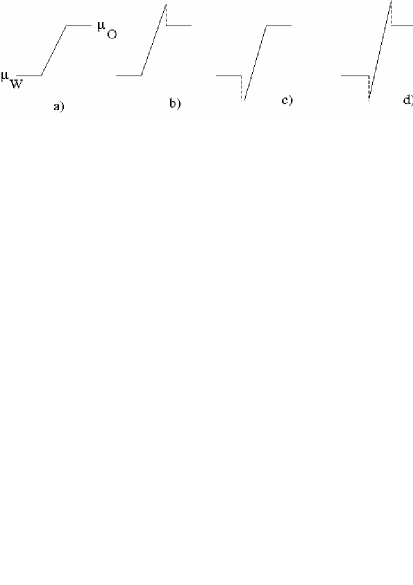
Figure 1: a) continuous linear viscosity between displacing fluid and oil; b), c), d): discontinuous linear viscosities with negative jumps in $x=0$ or (and) $x=-Q$.

Let $\mu_{min}$ be the smallest value of $\mu$ in the intermediate region, which can be less than $\mu_{W}$, as in Figures 1 c) - d). We have $\mu_{x}>0$, and from (48) we get

$$\sigma_{L}\leq U\frac{Max_{x}(\mu_{x})}{\mu_{min}}.$$ (49)

The above upper bound is not depending on the maximum value of the viscosity, but only on the maximum value of his derivative and on $\mu_{min}$.

Remark 3. The total (dimensional) amount $TA$ of liquid introduced in intermediate region is given by (see [13])

$$TA=\int_{-Q}^{0}\mu(x)dx.$$ (50)

We prove that $TA$ is the same for the viscosity profile given in Figure 1 a) and for the $N$ layer flow described by the formulas (36) - (37). For the linear profile the Figure 1a) we have

$$\int_{-Q}^{0}\mu(x)dx=(\mu_{W}+\mu_{O})Q/2$$

and for the $N$ layer viscosity profile (36) - (37) we obtain the same result:

$$\int_{-Q}^{0}\mu(x)dx=Q\mu_{O}-\sum_{i=N}^{i=1}i(\frac{\mu_{O}-\mu_{W}}{N+1})\frac{Q}{N}.$$

Remark 4. The linear continuous viscosity profile plotted in the Figure 1a) and the estimate (49) give us

$$\sigma_{LC}\leq U\frac{\mu_{O}-\mu_{W}}{Q\mu_{W}}.$$ (51)

Therefore we get an arbitrary small positive growth constant if $Q$ is large enough, even if both surface tensions in $x=-Q,\quad x=0$ are zero.

$\hfill\square$

We mention here that on the page 3 of  [29] is considered a linear viscosity profile in a porous medium.

6. Conclusions

The interface between two Newtonian immiscible fluids in a rectangular Hele-Shaw cell is unstable when the displacing fluid is less viscous. If the surface tension on the interface is zero, then the Saffman-Taylor growth constant of the linear perturbations is boundless with respect to the wave numbers $k$ - see the formula (24).

An intermediate fluid with a variable viscosity between the displacing fluid and oil can minimize the Saffman-Taylor instability when the surface tensions are different from zero - see the papers [12],  [13],  [14],  [15],  [16],  [17].

The multi-layer Hele-Shaw model, consisting of $N$ intermediate fluids with constant viscosities was studied in  [21],  [22], [23] , [24] and upper bounds of the growth rates were obtained. If all surface tensions are different from zero and verify some conditions, an arbitrary small (positive) upper bound of the growth rates can be obtained, if $N$ is large enough. This model is useless when all surface tensions on the interfaces are zero.

In this paper we study the Hele-Shaw displacement in rectangular cells, when all surface tensions on the interfaces are zero.

We point out a significant difference between the displacement with constant intermediate viscosities and the displacement with a single variable intermediate viscosity. In the first case, if the viscosity-jumps are positive in the flow direction, then the displacement process is unstable - see Proposition 2. In the second case we can almost suppress the Saffman-Taylor instability.

We get lower bounds of the growth rates in the three-layer case with constant intermediate viscosity - see Lemma 1 in section 3. We use this result for the case of $N$ intermediate constant-viscosity layers and get the lower bounds (40) and (45). Therefore the growth rates are unbounded with respect to the wave numbers of perturbations, as in the Saffman-Taylor case without surface tension.

In section 5 we study the three-layer case without surface tensions. An intermediate fluid with a linear increasing viscosity gives us arbitrary small (positive) growth constants if the middle region is large enough - see the formula (51).

The total amount of intermediate liquid for the $N$ layer flow given by (36), (37) and for the variable linear viscosity-profile given in Figure 1a) is the same - see Remark 3.

Our main conclusion is following. When all surface tensions are zero, the best strategy to minimize the Saffman-Taylor instability is to use an intermediate liquid with a suitable variable viscosity. On this way we can almost suppress the instability.

References

[1]
H. S. Hele-Shaw, Investigations of the nature of surface resistence of
water and of streamline motion under certain experimental conditions,
Inst. Naval Architects Transactions 40(1898), 21-46.
[2]H. Lamb, Hydrodynamics, Dower Publications, New York, 1933.
[3]
J. Bear, Dynamics of Fluids in Porous Media, Elsevier, New York, 1972.
[4]P.G. Saffman and G.I. Taylor, The penetration of a fluid in a porous medium
or Helle-Shaw cell containing a more viscous fluid, Proc. Roy. Soc.
A, 245 (1958), 312-329.
[5]P.G. Saffman, Viscous fingering in Hele-Shaw cells, J. Fl. Mech.,
173 (1986), 73-94.
[6]G.M. Homsy, Viscous fingering in porous media, Ann. Rev. Fluid Mech.,
19 (1987), 271-311.
[7]T. T. Al-Housseiny, P. A. Tsai, H. A. Stone,
Control of interfacial instabilities using flow geometry,
Nature Physics Letters, 8 (2012), 747–750.
[8]T. T. Al-Housseiny and H. A. Stone,
Controlling viscous fingering in Hele-Shaw cells,
Physics of Fluids, 25 (2013), pp. 092102.
[9]C.-Yao Chen, C.-W. Huang, L.-C. Wang, and José A. Miranda,
Controlling radial fingering patterns in miscible confined flows,
Phys. Rev. E, 82 (2010), pp. 056308.
[10]E.O. Diaz, A. Alvaez-Lacalle, M.S. Carvalho, Jose A. Miranda,
Minimization of viscous fluid fingering: a variational scheme for optimal flow rates,
Physical Review Letters, PRL 109 (2012), pp. 144502.
[11]B. Sudaryanto and Y. C. Yortsos,
Optimization of Displacements in Porous Media Using Rate Control,
Society of Petroleum Engineers,
Annual Technical Conference and Exhibition, 30 September-3 October, New Orleans, Louisiana
(2001).
[12]E. Gilje, Simulations of viscous instabilities in miscible and immiscible
displacement, Master Thesis in Petroleum Technology, University of
Bergen, 2008.
[13]S.B. Gorell and G.M. Homsy, A theory of the optimal policy of oil recovery by
secondary displacement process, SIAM J. Appl. Math.43 (1983),
79-98.
[14]S.B. Gorell and G. M. Homsy,
A theory for the most stable variable viscosity profile in graded mobility
displacement process, AIChE Journal, 31 (1985), 1598-1503.
[15]G. Shah and R. Schecter, eds., Improved Oil Recovery by Surfactants and
Polymer Flooding, Academic Press, New York, 1977.
[16]R.L. Slobod and S.J. Lestz, Use of a graded viscosity zone to reduce fingering
in miscible phase displacements, Producers Monthly, 24 (1960), 12-19.
[17]A.C. Uzoigwe, F.C. Scanlon, R.L. Jewett, Improvement in polymer flooding: The
programmed slug and the polymer-conserving agent, J. Petrol. Tech., 26 (1974),
33-41.
[18]P. Daripa and G. Pasa, On the growth rate of three-layer Hele-Shaw
flows - variable and constant viscosity cases, Int. J. Engng. Sci.,43 (2004), 877-884.
[19]P. Daripa and G. Pasa, New bounds for stabilizing Hele-Shaw flows,
Appl. Math. Lett., 18 (2005), 12930-1303.
[20]P. Daripa and G. Pasa, A simple derivation of an upper bound in the
presence of viscosity gradient in three-layer Hele-Shaw flows, J. Stat.
Mech., P 01014 (2006).
[21]P. Daripa, Hydrodynamic stability of multi-layer Hele-Shaw flows,
J. Stat. Mech., Art. No. P12005 (2008).
[22]P. Daripa and X. Ding, Universal stability properties for Multi-layer Hele-Shaw
flows and Applications to Instability Control, SIAM J. Appl. Math.,
72 (2012), 1667-1685.
[23]P. Daripa and X. Ding, A Numerical Study of Instability Control for the Design of an
Optimal Policy of Enhanced Oil Recovery by Tertiary Displacement Processes,
Tran. Porous Media93(2012), 675-703.
[24]P. Daripa, Some Useful Upper Bounds for the Selection of Optimal Profiles,
Physica A: Statistical Mechanics and its Applications391 (2012). 4065-4069.
[25]P.J. Flory, Principles of Polymer Chemistry, Ithaca, New York, Cornell
University Press, 1953.
[26]N. Mungan, Improved waterflooding through mobility control,
Canad J. Chem. Engr., 49 (1971), 32-37.
[27]L. Talon , N. Goyal and E. Meiburg,
Variable density and viscosity, miscible displacements in horizontal
Hele-Shaw cells. Part 1. Linear stability analysis,
J. Fluid Mech, 721 (2013), 268-294.
[28]D. Loggia, N. Rakotomalala, D. Salin and Y. C. Yortsos,
The effect of mobility gradients on viscous instabilities in miscible
flows in porous media, ̵́
Physics of Fluids, 11 (1999), 740-742.
[29]U. S. Geological Survey, Applications of SWEAT to select Variable-Density and Viscosity
Problems, U. S Department of the Interior, Specific Investigations Report 5028 (2009).