Comparison of RNN Encoder-Decoder Models for Anomaly Detection

Abstract

In this paper, we compare different types of Recurrent Neural Network (RNN) Encoder-Decoders in anomaly detection viewpoint. We focused on finding the model that can learn the same data more effectively. We compared multiple models under the same conditions, such as the number of parameters, optimizer, and learning rate. However, the difference is whether to predict the future sequence or restore the current sequence. We constructed the dataset with simple vectors and used them for the experiment. Finally, we experimentally confirmed that the model performs better when the model restores the current sequence, rather than predict the future sequence.

1 Introduction

Currently, the Recurrent Neural Network (RNN) used to generating sequence based on the input sequence. The sequence generation model based on RNN generally called sequence to sequence RNN or RNN Encoder-Decoder (RED) [1, 2]. In this paper, our purpose is finding the model that can learn the same data more effectively. We assumed the RED will be used for anomaly detection such as previous researches [3, 4, 5]. In their research, they were presented the model of predicting the future sequence from the current sequence. We wondered whether it is the best way to using future prediction model for anomaly detection. Because, we think restoring the current sequence is easier than predicting the future.

We compared three RED models. The first model is the future prediction model. The second model is modified model of the future prediction model to restoring current sequence. The last model is an intermediate model of the previous two models. The detail of each model is described in Section 2. In Section 3, we present our dataset and experimental result and conclude in the final section.

2 RNN Encoder-Decoder

The RNN Encoder-Decoder (RED) have similarities with Auto-Encoder (AE) that generate the output from the inputs. The RED used to predict the next sequences in general. For example, Sucheta Chauhan et al. used RED for anomaly detection in Electrocardiography (ECG) [3]. Their RED was trained to predict the next (future) $L$ sequences from the input sequences. The ECG consists by $P$, $Q$, $R$, $S$ and $T$ waveforms with repeating. Each waveform has the one-to-one correspondence in ECG. That means only the wave $Q$ wave can appear after the $P$. So, there is no problem for training or predicting with previous RED. However, if the next wave of wave $P$ is not only $Q$ but also $R$, $S$ and $T$ appears directly (one-to-many correspondence), it makes confusing to learning. The RED derives the output by causality shown in Equation 1 to 5. When the model receives input sequence that starting with $P$, RED becomes confused to select output among various options. Because the first vector of the output sequence is determined only by the first vector of the input sequence without the prior information. We experimented with the above attributes of RED.

$$i_{t}=\sigma(W_{i}x_{t}+U_{i}h_{t-1}+b_{i})$$ (1)

$$o_{t}=\sigma(W_{o}x_{t}+U_{o}h_{t-1}+b_{o})$$ (2)

$$f_{t}=\sigma(W_{f}x_{t}+U_{f}h_{t-1}+b_{f})$$ (3)

$$c_{t}=f_{t}\circ c_{t-1}+i_{t}\circ tanh(W_{c}x_{t}+U_{c}h_{t-1}+b_{c})$$ (4)

$$h_{t}=o_{t}\circ tanh(c_{t})$$ (5)

2.1 Models for comparison

In the RED, each RNN cell can be selectively used among vanilla RNN [6], Long-short Term Memory (LSTM) [7] and Gated Recurrent Unit (GRU) [8]. The vanilla RNN has vanishing gradient problem when the length of the sequence becomes long. However, LSTM and GRU solved vanishing gradient problem.

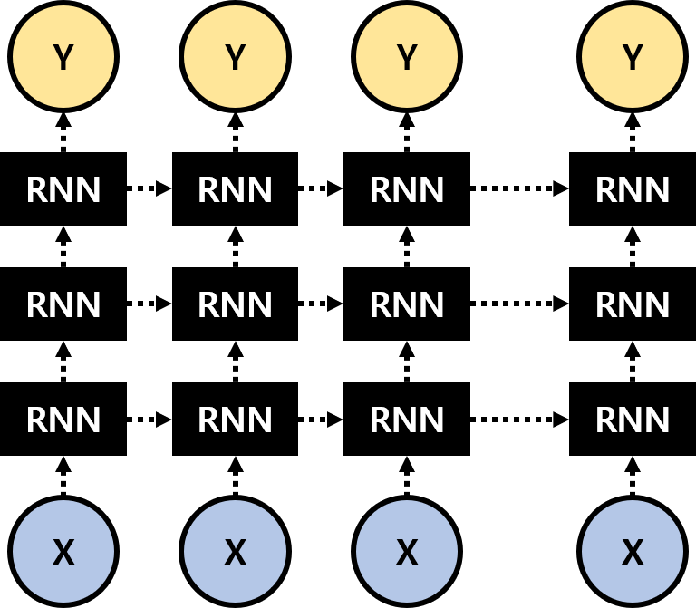
Figure 1: The RED architecture. It generates sequential output from sequential input.

We construct REDs using LSTM shown as Figure 1. Because, there is no superiority between LSTM and GRU that Chung et al. have already confirmed [9]. The relationship of input and output sequence can be adjusted for purpose. The relationship between the input and output was current $L$ sequence and future $L$ sequence in previous researches. In that case, RED learned to generate (predict) the future sequence from the current sequence.

$$p(\mathbf{Y}|\mathbf{X})\propto{p(\mathbf{X}|\mathbf{Y})p(\mathbf{Y})}$$ (6)

In the Equation 6, $\mathbf{X}$ and $\mathbf{Y}$ are input and output sequence respectively. The $p(\mathbf{Y}|\mathbf{X})$ is the uncertainty, $p(\mathbf{X}|\mathbf{Y})$ is likelihood and $p(\mathbf{Y})$ is prior knowledge. The RED will be learned $p(\mathbf{X}|\mathbf{Y})$ by the maximum likelihood estimation in the training process. If $\mathbf{X}$ and $\mathbf{Y}$ are almost the same, it will be easier to learn likelihood, but vice versa. Because, it is easier to get the $A^{\prime}$ than to get $B$ from the information $A$.

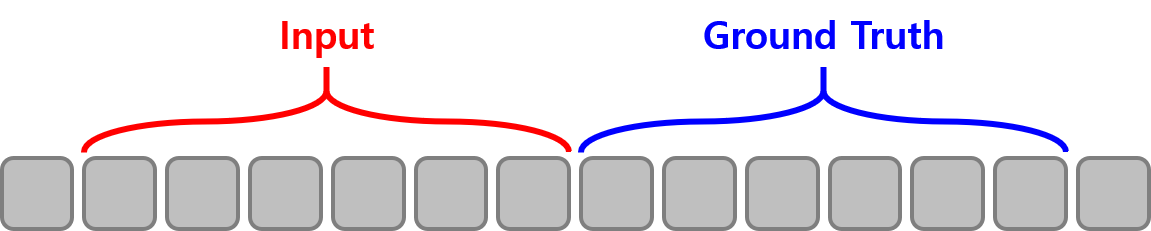
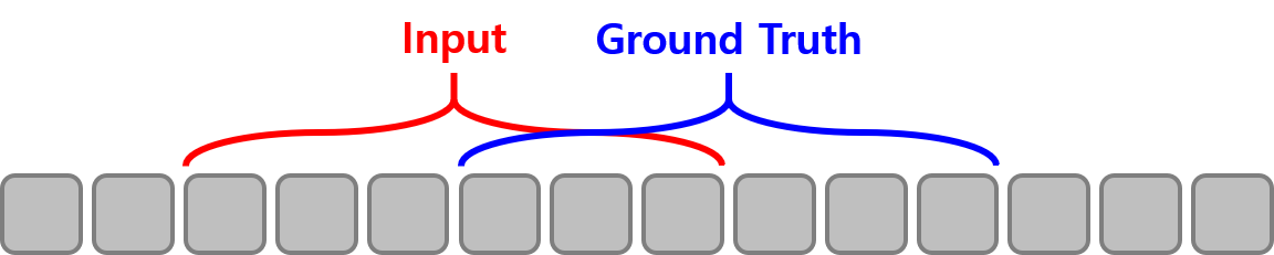
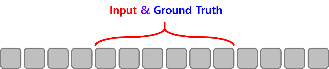
Figure 2: The RED models for comparison. We call these Model-A, Model-B and Model-C from the top.

We construct three models for experiment. Model-A is future prediction model that same as the model in the previous researches [3, 4, 5]. Model-C is restoration model that generates output sequence same as input sequence. Model-B is an intermediate model of Model-A and Model-C. We assume that the Model-C will be better to train when the dataset has one-to-many correspondence as mentioned earlier.

3 Experiment

In this section, we experimentally compare the three RED models. We constructed the simple sequential dataset for the experiment that described in Section 3.1.

3.1 Dataset

We constructed the dataset with 15 simple vectors. We called each vector $A$ (Alpha) to $O$ (Oscar) in North Atlantic Treaty Organization (NATO) phonetic alphabet and converted it to the one-hot encoded vector shown as Equation 7.

$$\begin{bmatrix}A\\ B\\ C\\ \vdots\\ O\end{bmatrix}=\begin{bmatrix}1&0&0&0&\dots&0\\ 0&1&0&0&\dots&0\\ 0&0&1&0&\dots&0\\ \vdots&&&&\ddots&\vdots\\ 0&0&0&0&\dots&1\\ \end{bmatrix}$$ (7)

We constructed three datasets with 15 vectors shown in Equation 7. One of the datasets consists of 5 vectors between $A$ to $E$ (Echo) and other datasets are consisting of whole 15 vectors. The pattern of each dataset is shown in Table 1. The patterns of each dataset are shown in Table 1 repeated for a length of 3000. The notable point of three datasets in Table 1 is Alpha symbol of Set-C. The symbol Alpha appears in front of symbol $B$ (Bravo), $D$ (Delta), $F$ (Foxtrot), $H$ (Hotel) and $J$ (Juliett). That makes confusing when training the pattern to RED because RED cannot generate the output correctly when the sequence started with Alpha.

Table 1: Three datasets for training process. Each pattern is repeating itself.

Dataset	Pattern	Length
Set-A	ABCDE	5
Set-B	ABCDEFGHIJKLMNO	15
Set-C	ABCADEAFGAHIAJK	15

Each dataset is subdivided into four types. One of subset consists of the same pattern as Table 1 and another one is added random noise to the original pattern with. Also, the dataset contains the new pattern that has not seen in Table 1 and added noise to them. We call each subset as ’Clear’, ’Noise’, ’Abnormal’ and ’Abnoise’ (abnormal with noise). Subset ’Clear’ and ’Noise’ is normal class and others are abnormal class. We use only one normal class subset of the all subsets for training. The test process uses all subsets.

3.2 Comparison

We compared the three models with three datasets. We trained each model with subset ’Clear’ and ’Noise’ respectively. We defined the synchronous case when the length of the pattern and the sequence length are equal or integer multiple. And other cases to asynchronous. We experimented with three synchronous cases and three asynchronous cases. Loss graphs of training process is shown in A. We evaluated three models with training set to confirm they learned well about the training set. Table 2 and 3 shows the result of evaluation. The lower loss means the model generates output more correctly. Model-C has lower loss than other models for all the training set.

Table 2: Loss matrix with training set. Each model trained with subset ’clear’.

Dataset (Subset)	Model-A	Model-B	Model-C
Set-A (Clear)	3.291	3.440	2.484
Set-B (Clear)	2.680	2.974	2.377
Set-C (Clear)	2.851	3.019	2.672

Table 3: Loss matrix with training set. Each model trained with subset ’noise’.

Dataset (Subset)	Model-A	Model-B	Model-C
Set-A (Noise)	5.253	5.380	4.771
Set-B (Noise)	4.615	4.888	4.378
Set-C (Noise)	4.781	4.844	4.499

We also evaluated three models with the test set shown as Table 4 and 5. Tables are presented the average loss for each class and model. The loss was measured by a divided normal set and abnormal set in each the test set. The lower loss for the normal set is better same as evaluation with the training set and for the abnormal set is vice versa.

Table 4: Loss matrix with test set. Each model trained with subset ’Clear’.

Dataset	Class	Model-A	Model-B	Model-C
Set-A	Normal	4.046	4.184	3.339
	Abnormal	5.180	5.238	4.484
Set-B	Normal	3.482	3.698	3.170
	Abnormal	4.351	4.554	3.955
Set-C	Normal	3.534	3.704	3.392
	Abnormal	4.929	4.905	4.116

Table 5: Loss matrix with test set. Each model trained with subset ’Noise’.

Dataset	Class	Model-A	Model-B	Model-C
Set-A	Normal	4.012	4.198	3.452
	Abnormal	5.169	5.353	4.571
Set-B	Normal	3.544	3.825	3.285
	Abnormal	4.365	4.603	3.285
Set-C	Normal	3.691	3.752	3.392
	Abnormal	4.961	4.874	4.103

Since confirming the superiority only with the loss value is difficult, we also checked the generated sequence. We present the part of the test case in Table 6 and 7. We provide the whole test result in our Github repository .

Table 6: The part of test result with Set-A. The sequence length is 3 (asynchronous case) and each model trained with subset ’Clear’.

Model	Subset	Input	Output	Ground-Truth	Loss
Model-A	Clear	ABC	DEA	DEA	0.244
	Noise	DEA	BCD	BCD	1.480
	Abnormal	BDE	EAB	ACC	2.106
	Abnoise	BBC	EAA	DEB	1.926
Model-B	Clear	ABC	BCD	BCD	0.244
	Noise	DEA	EAB	EAB	1.104
	Abnormal	BDE	CDA	DEA	1.794
	Abnoise	BBC	CDE	BCD	2.283
Model-C	Clear	ABC	ABC	ABC	0.244
	Noise	DEA	DEA	DEA	1.261
	Abnormal	BDE	BCD	BDE	1.707
	Abnoise	BBC	BCC	BBC	1.747

Table 7: The part of test result with Set-C. The sequence length is 8 (asynchronous case) and each model trained with subset ’Clear’.

Model	Class	Input	Output	Ground-Truth	Loss
Model-A	Clear	ABCADEAF	EAHIAJKA	GAHIAJKA	0.913
	Noise	AFGAHIAJ	DABCADEA	KABCADEA	2.169
	Abnormal	JKBBBADE	AFGAHIAJ	AFGAHIAJ	0.243
	Abnoise	AKKKBCAD	DAFGAHIA	EAFGAHIK	2.468
Model-B	Clear	ABCADEAF	BEAFGAHI	DEAFGHAI	0.917
	Noise	AFGAHIAJ	JIAJKABC	HIAJKAVC	2.100
	Abnormal	JKBBBADE	CADEAAGA	BADEAFGA	1.944
	Abnoise	AKKKBCAD	JAAAEAJA	BCADEAFG	3.119
Model-C	Clear	ABCADEAF	ABCADEAF	ABCADEAF	0.241
	Noise	AFGAHIAJ	AFGAHIAJ	AFGAHIAJ	1.673
	Abnormal	JKBBBADE	JKABBADE	JKBBBADE	1.268
	Abnoise	AKKKBCAD	AKAKBCAD	AKKKBCAD	2.818

Each model generates the output sequences correctly when it received normal sequences, but it cannot generate the output correctly when it received abnormal sequences as shown in Table 6. We use this property for anomaly detection. However, we confirmed in Table 7, Model-A did not correctly predict the next sequence when using Set-C whether the input was normal or abnormal. Model-A may be performing a high recall for anomaly detection, but it can be always decided the state to abnormal. Model-C correctly restore the input sequence as output when it receipted normal sequences.

Table 8: The part of test result with Set-C. The sequence length is 8 (asynchronous case) and each model trained with subset ’Noise’.

Model	Class	Input	Output	Ground-Truth	Loss
Model-A	Clear	ABCADEAF	CAHIAJKA	GAHIAJKA	1.986
	Noise	AFGAHIAJ	CABCADEA	KABCADEA	0.858
	Abnormal	JKBBBADE	AFGAHIAJ	AFGAHIAJ	1.794
	Abnoise	AKKKBCAD	CFFGAHIA	EAFGAHIK	2.006
Model-B	Clear	ABCADEAF	JEAFGAHI	DEAFGHAI	2.018
	Noise	AFGAHIAJ	FIAJKABC	HIAJKAVC	0.900
	Abnormal	JKBBBADE	CADEAFGA	BADEAFGA	2.412
	Abnoise	AKKKBCAD	FAAADAFG	BCADEAFG	2.263
Model-C	Clear	ABCADEAF	ABCADEAF	ABCADEAF	1.996
	Noise	AFGAHIAJ	AFGAHIAJ	AFGAHIAJ	0.283
	Abnormal	JKBBBADE	JKABBIDE	JKBBBADE	2.699
	Abnoise	AKKKBCAD	AKKKACAD	AKKKBCAD	1.213

Table 8 shows part of the test results when each model trained with subset ’Noise’. Model-A and Model-B cannot predict the next sequences correctly when using the subset ’Clear’ unlike Table 7, but Model-C is not. Model-A constructed for focused on predicting future sequences rather than current key features. However, since Model-C constructed to restore current sequences, it can concentrate on learning key features in a given pattern. So, Model-C can get the robustness whether noise is added to the sequence.

4 Conclusion

We experimentally compared the three models of RED. We assume the RED are used for anomaly detection. The RED generates or predicts the next sequences in general. But we wondered whether the future predicting is the best way for anomaly detection. There is no difference in predicting future time $t$, determining anomalies, and restoring and immediately determining the current state. The only difference is the difficulty of the training process.

The model selection and setting of the sequence length are not important when the sequential vector has one-to-one correspondence property. But that case is a very ideal, and it is almost rare. There is a probability that various pattern appears randomly after the specific pattern like Set-C in reality. It is possible to get the correct result by an irregular pattern like Set-C by accident, but it is usually difficult.

We presented in the Section 3.2, Model-C learned the same data more easily and effectively than other models. We certain restoring the current sequence like Model-C is better than predicting the future sequence like Model-A and Model-C for anomaly detection. The smoother the training process means it can performing better, and we have confirmed it with experiment.

When using the Model-A for anomaly detection, it will face the problem of misjudging the normal state as abnormal. The Model-C does not make correct judgments absolutely, but at least it will perform much better than other models. Also, we expect the Model-C can be using other types of time series data generation problems and performing well.

5 References

Appendix A

A contains loss graphs of training process. Each process was performed with three models and three datasets respectively. Left side of each figure presents the synchronous case and the right side is the asynchronous case. Firstly, we show the results of the training process with subset ’Clear’. Last three figures are results of the training process with subset ’Noise’.

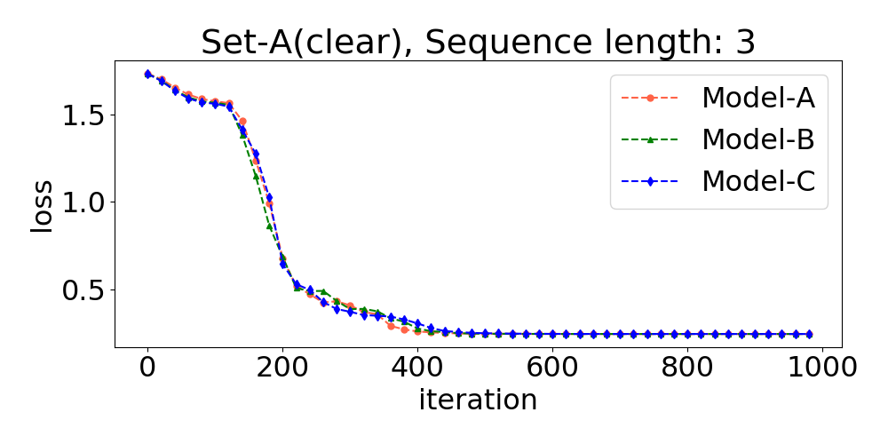
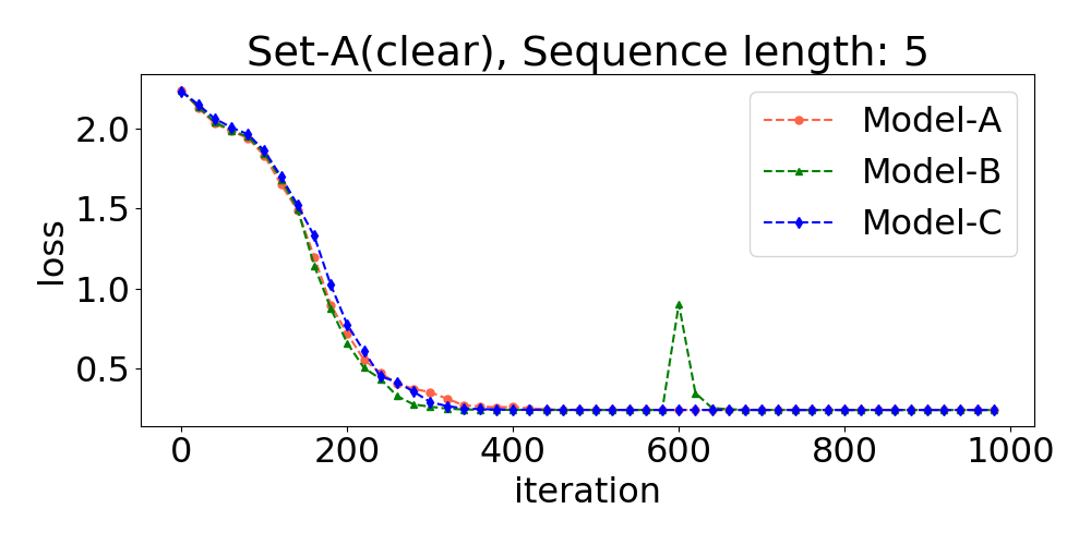
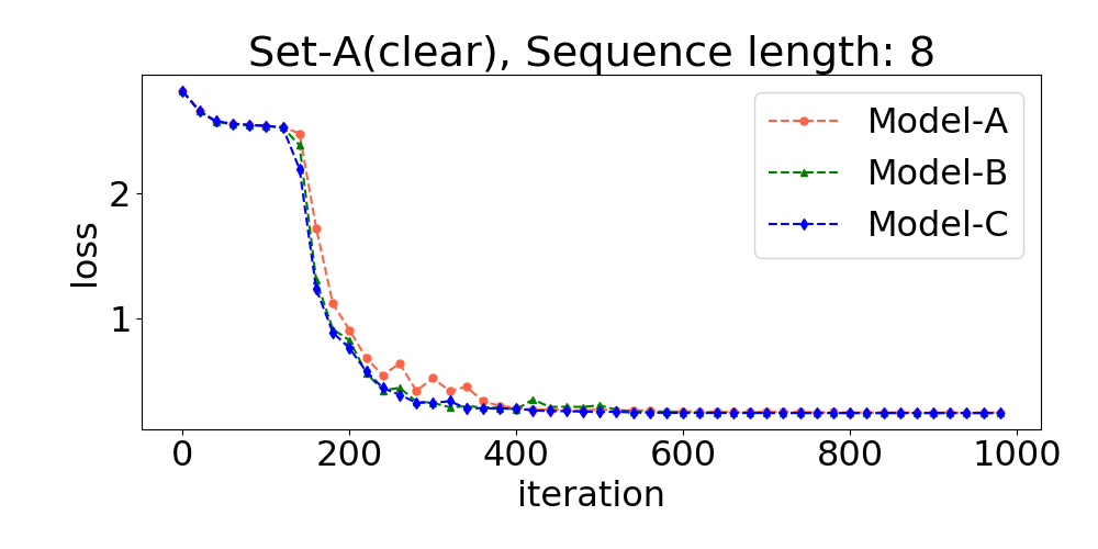
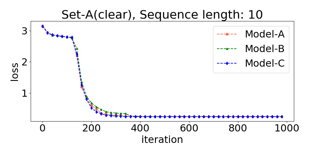
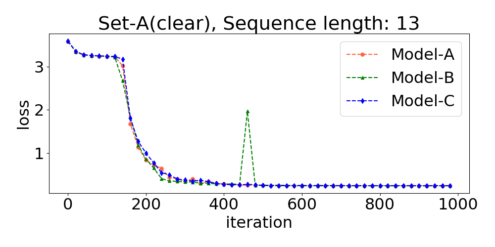
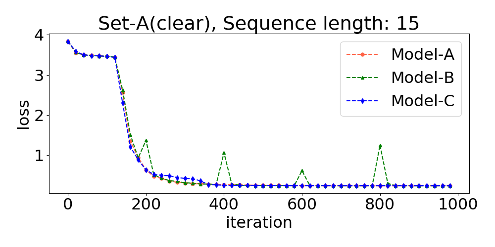
Figure 3: Loss graph of training process with subset ’Clear’ of the Set-A. Loss value of each model converged almost similar moment at each sequence length.

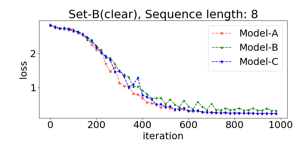
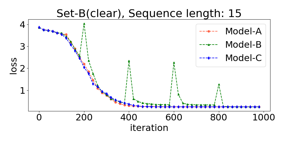
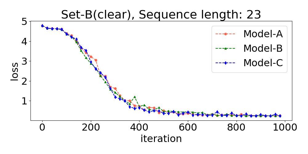
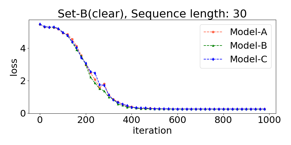
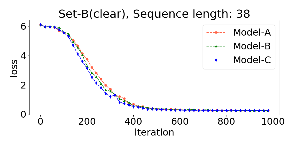
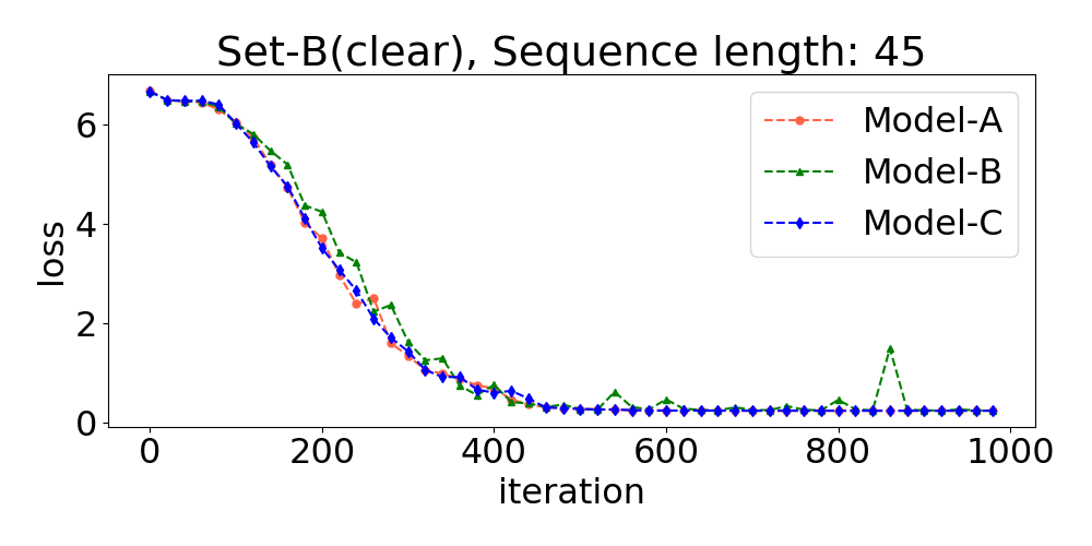
Figure 4: Loss graph of training process with subset ’Clear’ of the Set-B.

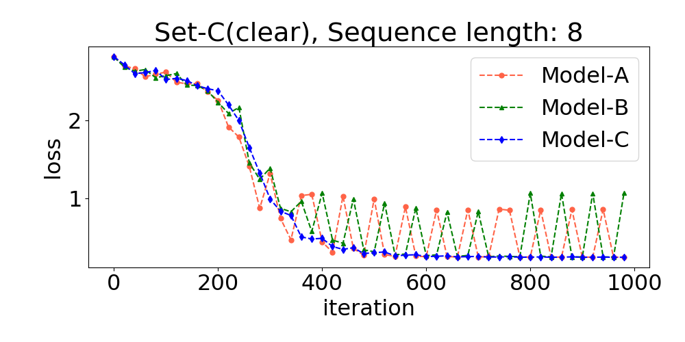
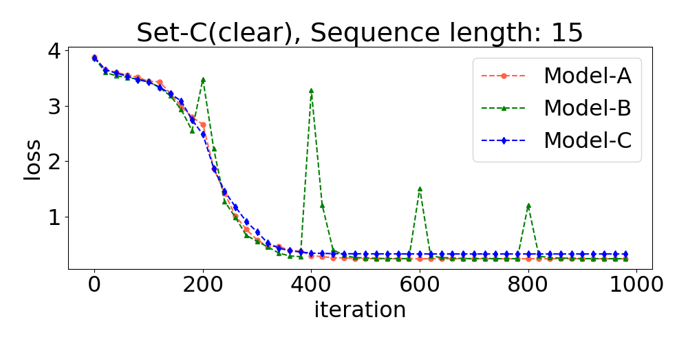
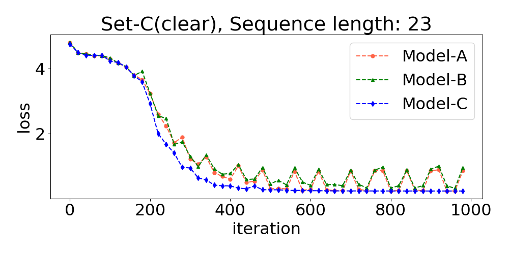
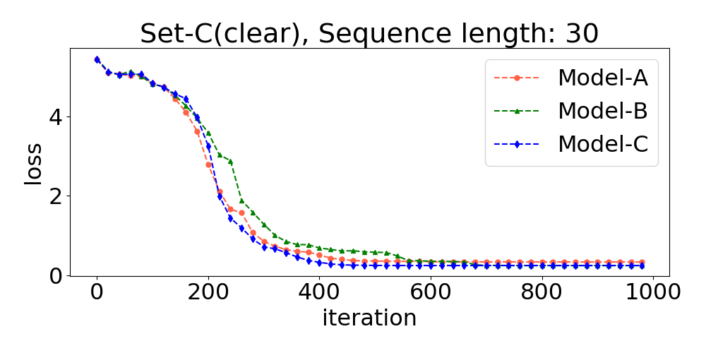
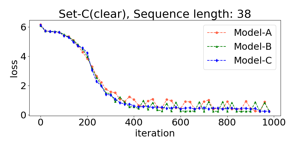
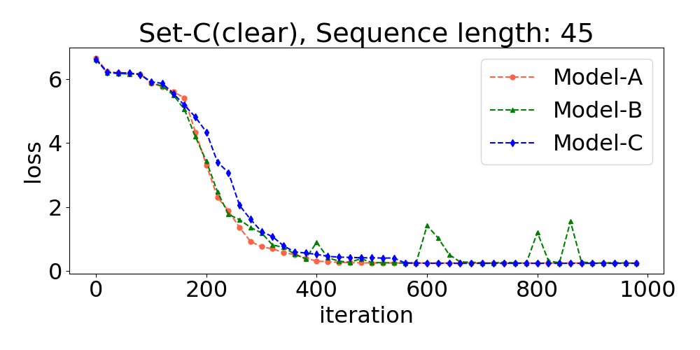
Figure 5: Loss graph of training process with subset ’Clear’ of the Set-C. The loss value of Model-A and Model-B oscillated in asynchronous cases but Model-C is not.

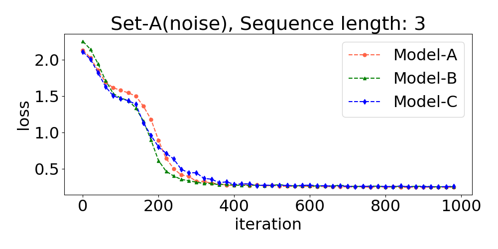
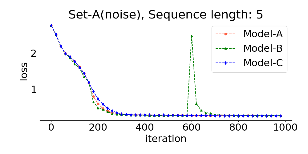
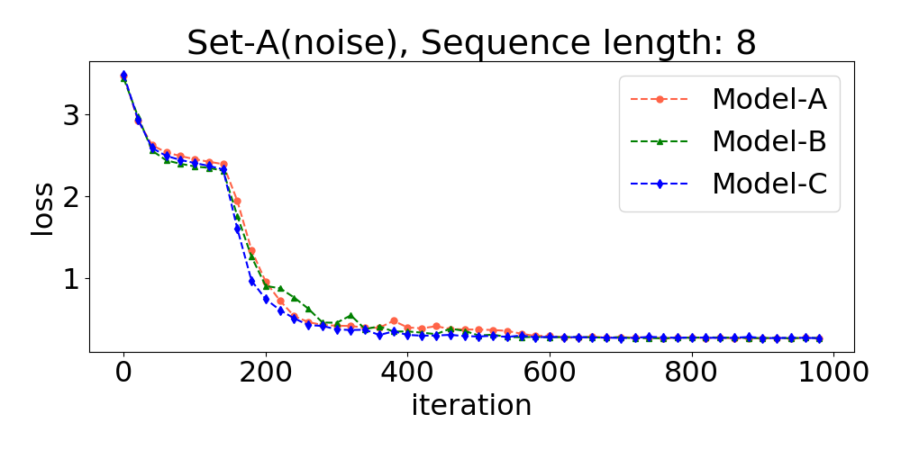
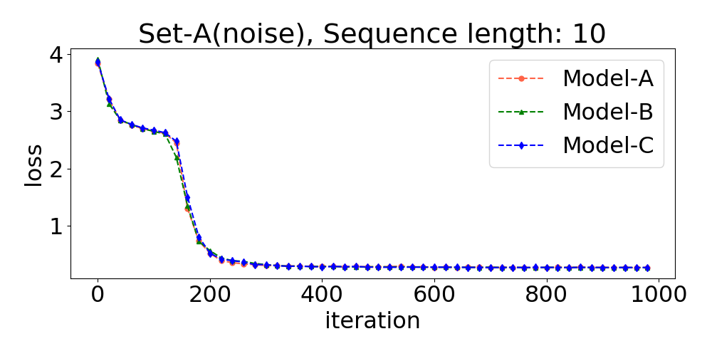
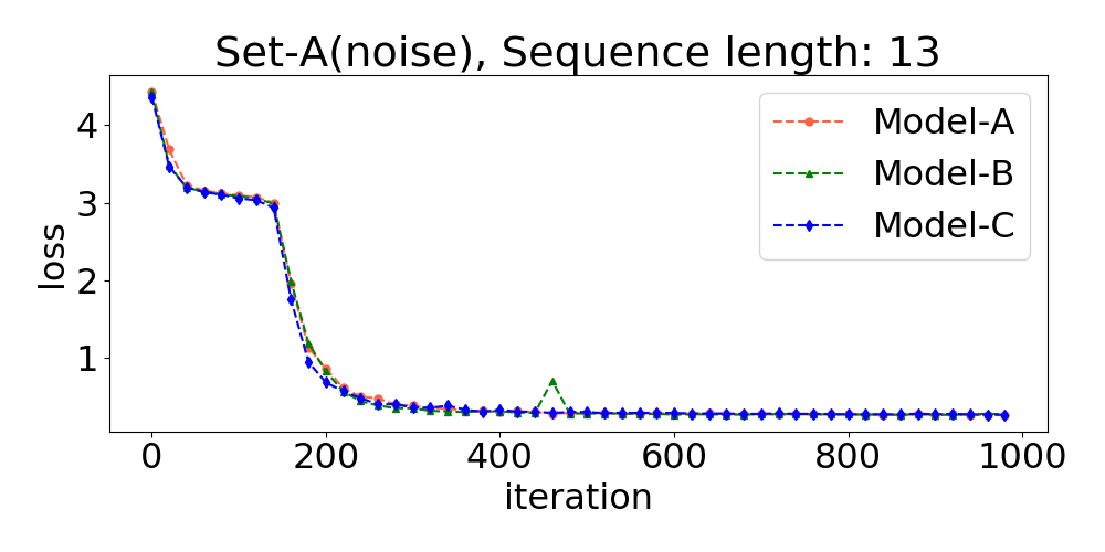
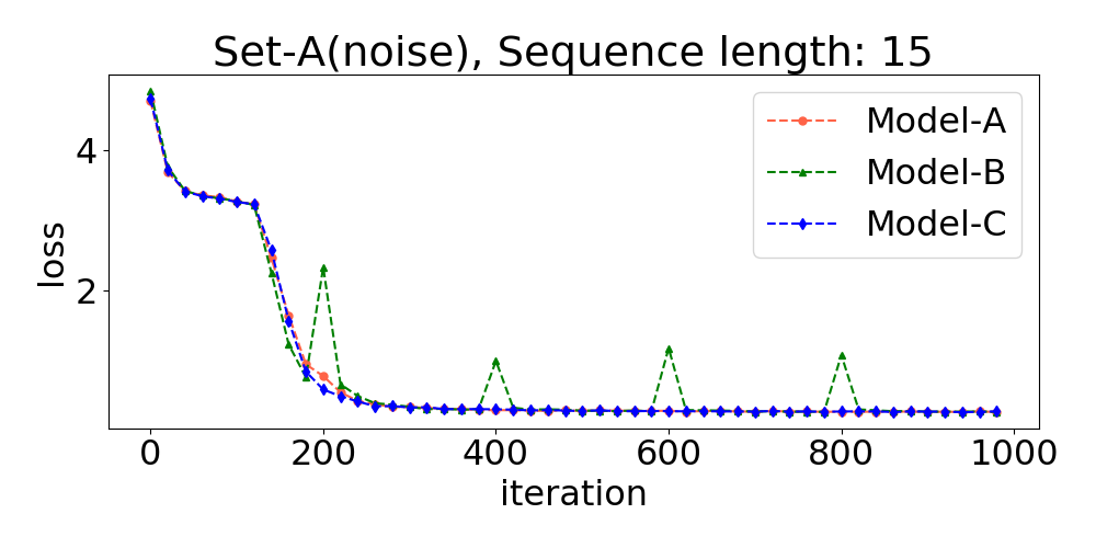
Figure 6: Loss graph of training process with subset ’Noise’ of the Set-A.

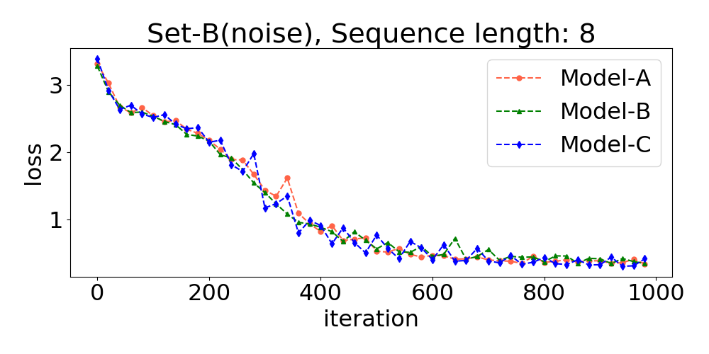
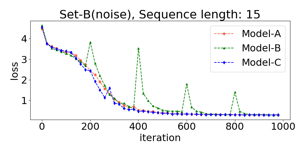
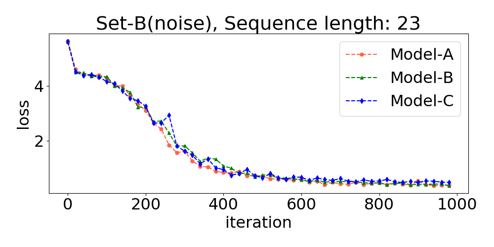
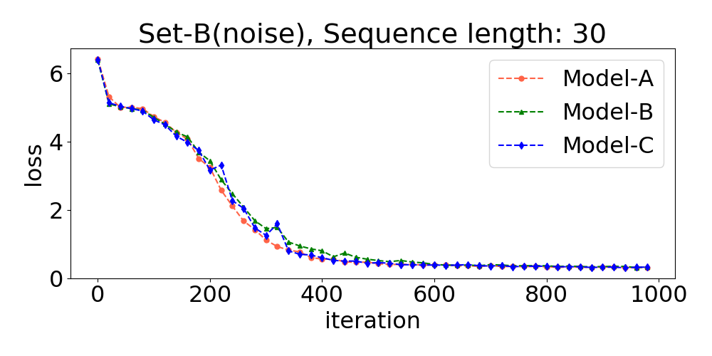
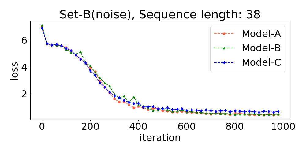
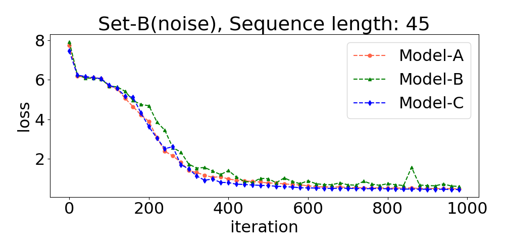
Figure 7: Loss graph of training process with subset ’Noise’ of the Set-B.

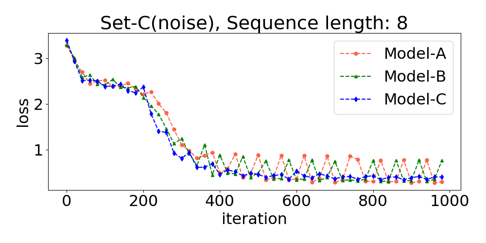
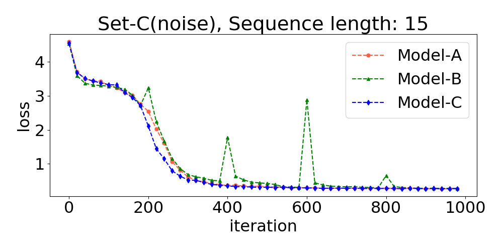
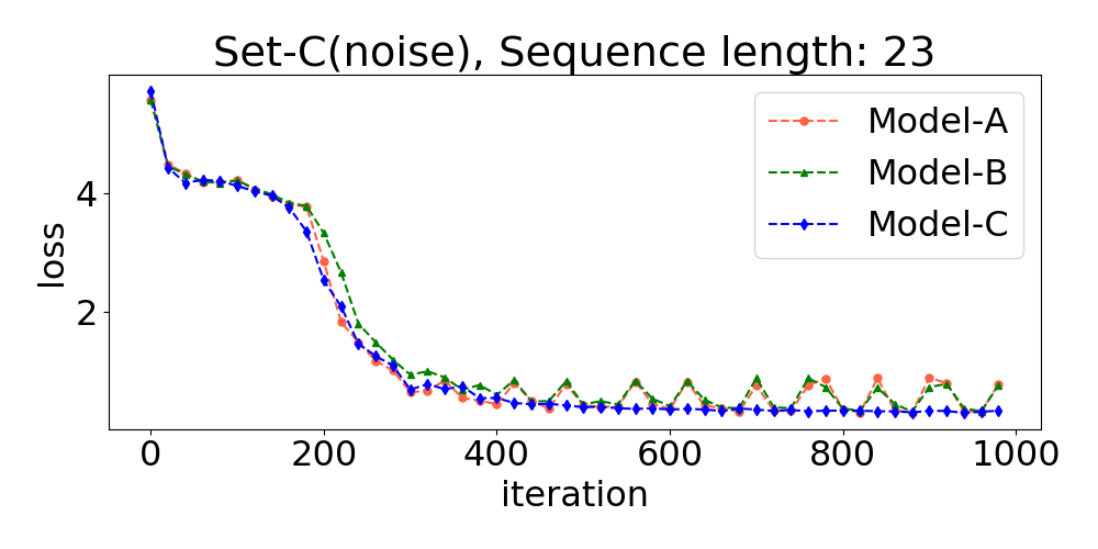
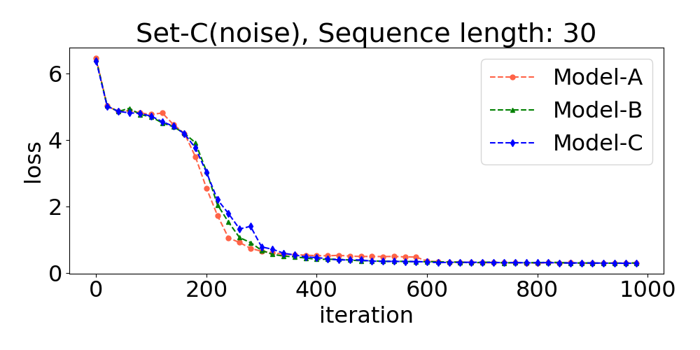
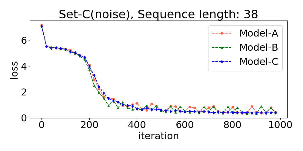
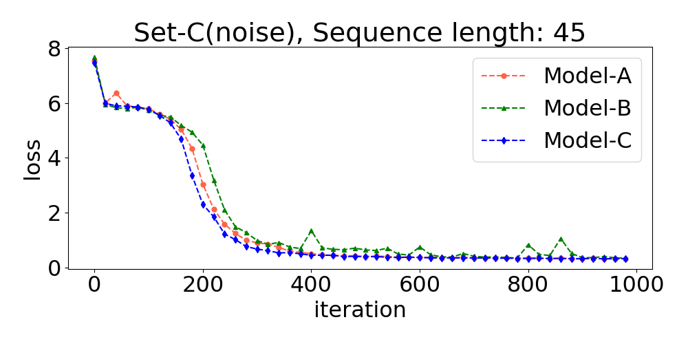
Figure 8: Loss graph of training process with subset ’Noise’ of the Set-C.

References

- [1] I. Sutskever, O. Vinyals, Q. V. Le, Sequence to sequence learning with neural networks, Advances in neural information processing systems pp. 3104-3112
- [2] K. Cho, B. Van Merriënboer, C. Gulcehre, D. Bahdanau, F. Bougares, H. Schwenk, Y. Bengio, Learning phrase representations using rnn encoder-decoder for statistical machine translation, arXiv preprint arXiv:1406.1078.
- [3] S. Chauhan, L. Vig, Anomaly detection in ECG time signals via deep long short-term memory networks, Data Science and Advanced Analytics (DSAA), 2015. 36678 2015. IEEE International Conference on, IEEE, pp. 1–7
- [4] P. Malhotra, L. Vig, G. Shroff, P. Agarwal, Long short term memory networks for anomaly detection in time series, in: Proceedings, Presses universitaires de Louvain, 2015, p. 89.
- [5] A. Nanduri, L. Sherry, Anomaly detection in aircraft data using Recurrent Neural Networks (RNN), Integrated Communications Navigation and Surveillance (ICNS), 2016, IEEE, pp. 5C2–1
- [6] T. Mikolov, M. Karafiát, L. Burget, J. Černockỳ, S. Khudanpur, Recurrent neural network based language model, in: Eleventh Annual Conference of the International Speech Communication Association
- [7] S. Hochreiter, J. urgen Schmidhuber, C. Elvezia, Long short-term memory, Neural Computation 9 (8) (1997) 1735–1780.
- [8] J. Chung, C. Gulcehre, K. Cho, Y. Bengio, Gated feedback recurrent neural networks, arXiv preprint arXiv:1502.02367.
- [9] J. Chung, C. Gulcehre, K. Cho, Y. Bengio, Empirical evaluation of gated recurrent neural networks on sequence modeling, arXiv preprint arXiv:1412.3555.