Using link and content over time for embedding generation in Dynamic Attributed Networks

Abstract

In this work, we consider the problem of creating an embedding combining link, content and temporal analysis for community detection and prediction in evolving networks. Such temporal and content-rich networks occur in many real-life settings, such as bibliographic networks and question answering forums. Most of the work in the literature (that uses both content and structure) deals with static snapshots of networks, and they do not reflect the dynamic changes occurring over multiple snapshots. Incorporating dynamic changes in the communities into the analysis can also provide useful insights about the changes in the network such as the migration of authors across communities. In this work, we propose Chimera, a shared factorization model that can simultaneously account for graph links, content, and temporal analysis. This approach works by extracting the latent semantic structure of the network in multidimensional form, but in a way that takes into account the temporal continuity of these embeddings. Such an approach simplifies temporal analysis of the underlying network by using the embedding as a surrogate. A consequence of this simplification is that it is also possible to use this temporal sequence of embeddings to predict future communities. We present experimental results illustrating the effectiveness of the approach.

I Introduction

Structural representations of data are ubiquitous in different domains such as biological networks, online social networks, information networks, co-authorship networks, and so on. The problem of community detection or graph clustering aims to identify densely connected groups of nodes in the network [10], one of the central tasks in network analysis. Examples of useful applications include that of finding clusters in protein-protein interaction networks [31] or groups of people with similar interests in social networks [39]. Recently, it has become easier to collect content-centric networks in a time-sensitive way, enabling the possibility of using tightly-integrated analysis across different factors that affect network structure. Aggregate topological and content information can enable more informative community detection, in which cues from different sources are integrated into more powerful models.

Another important aspect of complex networks is that such networks evolve, meaning that nodes may move from one community to another, making some communities grow, and others shrink. For example, authors that usually publish in the data mining community could move to the machine learning community. Furthermore, the temporal aspects of changes in community structure could interact with the content in unusual ways. For example, it is possible for an author in a bibliographic network to change their topic of work, preceding a corresponding change in community structure. The converse is also possible, with a change in community structure affecting content-centric attributes.

Matrix factorization methods are traditional techniques that allow us to reduce the dimensional space of network adjacency representations. Such methods have broad applicability in various tasks such as clustering, dimensionality reduction, latent semantic analysis, and recommender systems. The main point of matrix factorization methods is that they embed matrices in a latent space where the clustering characteristics of the data are often amplified. A useful variant of matrix factorization methods is shared matrix factorization, which factors two or more different matrices simultaneously. Shared matrix factorization is not new, and is used in various settings where different matrices define different parts of the data (e.g., links and content). This method could be used to embed link and content in a shared feature space, which is convenient because it allows the use of traditional clustering techniques, such as $k$-means. However, incorporating a temporal aspect to the shared factorization process adds some challenges concerning the adjustment of the shared factorization as data evolves.

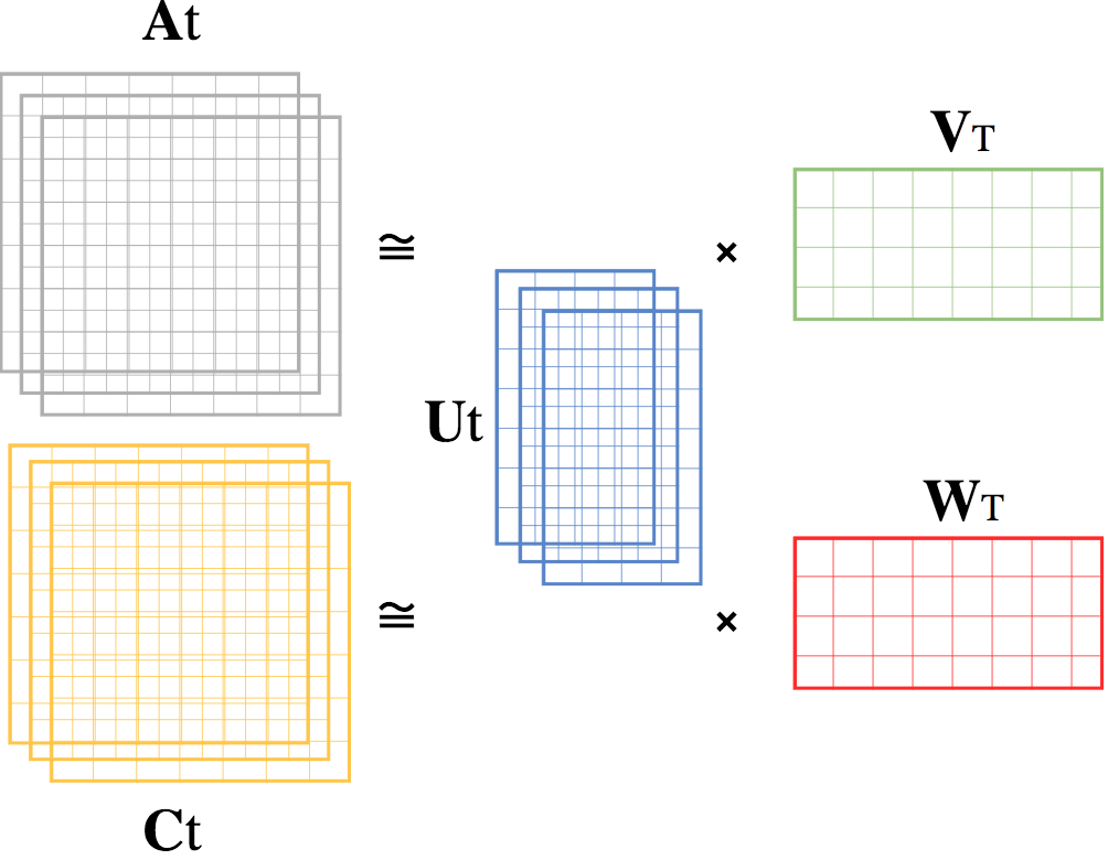
Figure 1: Graphical representation how shared factorization on Chimera works.

In Figure 1, we illustrate the broad principles of our approach. We factorize link and content over time at once. The matrix $U$ represents link and content in a shared dimension and each snapshot of time will have a different matrix $U$. These different values of the matrix $U$ provide insights at various temporal snapshots, and therefore they can be used for temporal community detection as shown in Figure 2.

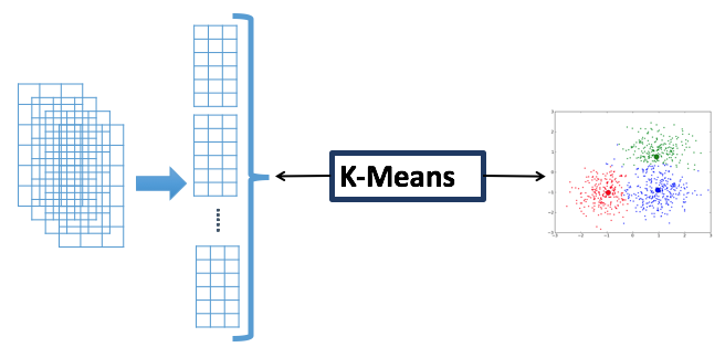
Figure 2: The different matrices corresponding to $U$ are condensed in one dataset to be clustered using the $k$-means algorithm.

Related to the problem of community detection is is that of community prediction, in which one attempts to predict future communities from previous snapshots of the network. It is notoriously difficult to predict future clustering structures from a complex combination of data types such as links and content. However, the matrix factorization methodology provides a nice abstraction, because one can now use the multidimensional representations created by sequences of matrices over different snapshots. The basic idea is that we can consider each of the entries in the latent space representation as a stream of evolving entries, which implicitly creates a time-series that can be used to predict future communities, as illustrated in Figure 3.

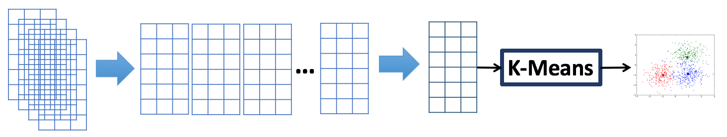
Figure 3: The different matrices corresponding to $U$ combine as a stream of data to predict future communities.

In this work, we present Chimera, a method that uses link and content from networks over time to detect and predict community structure. To the best of our knowledge, there is no work addressing these three aspects simultaneously for both detection and prediction of communities. The main contributions of this paper are:

• An efficient algorithm based on shared matrix factorization that uses link and content over time; the uniform nature of the embedding allows the use of any traditional clustering algorithm on the corresponding representation.

• A method for predicting future communities from embeddings over snapshots.

II Related Work

In this section, we review the existing work for community detection using link analysis, content analysis, temporal analysis and their combination. Since these methods are often proposed in different contexts (sometimes even by different communities), we will organize these methods into separate sections.

Topological Community Detection

These methods are based mainly on links among nodes. The idea is to minimize the number of edges across nodes belonging to different communities. Thus, the nodes inside the community should have a higher density (number of edges) with other nodes inside the community than with nodes outside the community. There are several ways of defining and quantifying communities based on their topology, modularity [4], conductance [22], betweeness [11], and spectral partition [1]. More can be found in [10].

Content-Centric Community Detection

Topic modeling is a common approach for content analysis and is often used for clustering, in addition to dimensionality reduction. PLSA-PHITS [15] and LDA [8] are the most traditional methods for content analysis, but they are susceptible to words that appear very few times. Extended methods that are more reliable are Link-PLSA-LDA [26] and Community-User-Topic model [43]. In most cases, the combination of link and content provides insights that are missing with the use of a single modality.

Link and Temporal Community Detection

A few authors address the problem of temporal community detection that aims to identify how communities emerge, grow, combine, and decay over time [23, 20], [6], [21], [38] use temporal Dirichlet processes to detect communities and track their evolution. [7] tackle the problem of overlapping temporal communities. [2] propose the detection of communities in temporal networks represented as multilayer networks. [30] identify clusters of nodes that are frequently connected for long periods of time, and such sets of nodes are referred to as temporal communities. [14] propose an algorithm for dynamic community detection in temporal networks, which takes advantage of community information at previous time steps. [42] present a model-based matrix factorization for link prediction and also for community prediction. However, their work uses only links for the prediction process.

Link and Content-Centric Community Detection

In recent years, some approaches were developed to use link and content information for community detection [33, 41, 24, 40]. Among them, probabilistic models have been applied to fuse content analysis and link analysis in a unified framework. Examples include generative models that combine a generative linkage model with a generative content-centric model through some shared hidden variables [9, 27]. A discriminative model is proposed by [41], where a conditional model for link analysis and a discriminative model for content analysis are unified. In addition to probabilistic models, some approaches integrate the two aspects from other directions. For instance, a similarity-based method [44] adds virtual attribute nodes and edges to a network, and computes the similarity based on the augmented network. [13] use matrix factorization to combine sources to improving tagging. It is evident that none of the aforementioned works combine all the three factors of link, content, and temporal information within a unified framework; caused in part by the fact that these modalities interact with one another in complex ways. Therefore, the use of latent factors is a particularly convenient way to achieve this goal.

Community Prediction

There has been a growing interest in the dynamics of communities in evolving social networks, with recent studies addressing the problem of building a predictive model for community detection. Most of the community prediction techniques described in these works are about community evolution prediction that aim to predict events such as growth, survival, shrinkage, splits and merges [19, 5, 28, 12, 37, 36, 34]. In [16, 18] the authors use ARIMA models to predict community events in a network without using any previous community detection method. [17] propose to use a small number of features to predict community events. [29] employ several structural and temporal features to represent communities and improve community evolution prediction.

The community prediction addressed in our work can predict not only community evolution but also a more accurate prediction about each node of the network, in which community the node will be and if its community will change or not. We do so by using topological characteristics and also content associated with nodes.

III Problem Definition

We assume we have $T$ graphs $G_{1}\ldots G_{T}$ that form a time-series. The graphs are defined over a fixed set of nodes $\mathcal{N}$ of cardinality $n$. In each timestamp, a different set of edges may exist over time. For example, in the case of a co-authorship network, the node set may correspond to the authors in the network, and the graph $G_{t}$ might correspond to the co-author relations among them in the $t$th year. These co-author relations are denoted by the $n\times n$ adjacency matrix $A_{t}$. Note that the entries in $A_{t}$ need not be binary, but might contain arbitrary weights. For example, in a co-authorship network, the entries might correspond to the number of publications between a pair of authors. For undirected graphs, the adjacency matrix $A_{t}$ is symmetric, while in directed graphs the adjacency matrix is asymmetric. Our approach can handle both settings. Hence, the graph $G_{t}$ is denoted by the pair $G_{t}=(\mathcal{N},A_{t})$.

We assume that for each timestamp $t$, we have an $n\times d$ content matrix $C_{t}$. $C_{t}$ contains one row for each node, and each row contains $d$ attribute values representing the content for that node at the $t$th timestamp. For example, in the case of the co-authorship network, $d$ might correspond to the lexicon size, and each row might contain the word frequencies of various keywords in the titles. Therefore, one can fully represent the content and structural pair at the $t$th timestamp with the triplet $(\mathcal{N},A_{t},C_{t})$.

In this paper, we study the problem of content-centric community detection in networks. We study two problems: temporal community detection, and community prediction. While the problem of temporal community detection has been studied in the literature, as presented in Section II, the problem of community prediction, as defined in this work, has not been studied to any significant extent. We define these problems as follows.

Definition 1 (Temporal Community Detection).

Given a sequence of snapshots of graphs $G_{1}\ldots G_{T}$, with $n\times n$ adjacency matrices $A_{1}\ldots A_{T}$, and $n\times d$ content matrices $C_{1}\ldots C_{T}$, create a clustering of the nodes into $k$ partitions at each timestamp $t\leq T$.

The clustering of the nodes at each timestamp $t$ may use only the graph snapshots up to and including time $t$. Furthermore, the clusters in successive timestamps should be temporally related to one another. Such a clustering provides better insights about the evolution of the graph. In this sense, the clustering of the nodes for each timestamp will be somewhat different from what is obtained using an independent clustering of the nodes at each timestamp.

Definition 2 (Temporal Community Prediction).

Given a sequence of snapshots of graphs $G_{1}\ldots G_{T}$ with $n\times n$ adjacency matrices $A_{1}\ldots A_{T}$, and $n\times d$ content matrices $C_{1}\ldots C_{T}$, predict the clustering of the nodes into $k$ partitions at future timestamp $T+r$.

The community prediction problem attempts to predict the communities at a future timestamp, before the structure of the network is known. To the best of our knowledge, this problem is new, and it has not been investigated elsewhere in the literature. Note that the temporal community prediction problem is more challenging than temporal community detection, because it requires us to predict the community structure of the nodes without any knowledge of the adjacency matrix at that timestamp.

Temporal prediction is generally a much harder problem in the structural domain of networks as compared to the multidimensional setting. In the multidimensional domain, one can use numerous time-series models such as the auto-regressive (AR) model to predict future trends. However, in the structural domain, it is far more challenging to make such predictions.

IV Mathematical Model

In this section, we discuss the optimization model for converting the temporal sequences of graphs and content to a multidimensional time-series. To achieve this goal, we use a non-negative matrix factorization framework. Although the non-negativity is not essential, one advantage is that it leads to a more interpretable analysis. Consider a setting in which the rank of the factorization is denoted by $k$. The basic idea is to use three sets of latent factor matrices in a shared factorization process, which is able to combine content and structure in a holistic way:

1. The matrix $U_{t}$ is an $n\times k$ matrix, which is specific to each timestamp $t$. Each row of the matrix $U_{t}$ describes the $k$-dimensional latent factors of the corresponding node at time stamp $t$, while taking into account both the structural and content information.

2. The matrix $V$ is an $n\times k$ matrix, which is global to all timestamps. Each row of the matrix $V$ describes the $k$-dimensional latent factors of the corresponding node over all time stamps, based on only the structural information.

3. The matrix $W$ is an $d\times k$ matrix, which is global to all timestamps. Each row of the matrix $W$ describes the $k$-dimensional latent factors of one of the $d$ keywords over all time stamps, based on only the content information.

The matrices $U_{1}\ldots U_{T}$ are more informative than the other matrices, because they contain latent information specific to the content and structure, and they are also specific to each timestamp. However, the matrices $V$ and $W$ are global, and they contain only information corresponding to the structure and the content in the nodes, respectively. This is a setting that is particularly suitable to shared matrix factorization, where the matrices $U_{1}\ldots U_{T}$ are shared between the factorization of the adjacency and content matrices.

Therefore, we would like to approximately factorize the adjacency matrices $A_{1}\ldots A_{T}$ as $A_{t}\approx U_{t}V^{T}$, for all $t\in\{1\ldots T\}$. Similarly, we would like to approximately factorize the content matrices $C_{1}\ldots C_{T}$ as $C_{t}\approx U_{t}W^{T}$. With this setting, we propose the following optimization problem:

$$J =\sum_{t=1}^{T}\left\|A_{t}-U_{t}V^{T}\right\|^{2}+\beta\sum_{t=1}^{T}\left\|C_{t}-U_{t}W^{T}\right\|^{2}$$ (1)

$$+\lambda_{1}\Omega(U_{t},V,W)\,\text{.}$$

Where $\beta$ is a balancing parameter, $\lambda_{1}$ is the regularization parameter, and $\Omega(U_{t},V,W)$ is a regularization term to avoid overfitting. The notation $\|\cdot\|^{2}$ denotes the Frobenius norm, which is the sum of the squares of the entries in the matrix. The regularization term is defined as

$$\Omega(U_{t},V,W)=\|V\|^{2}+\|W\|^{2}+\sum_{t=1}^{T}\left\|U_{t}\right\|^{2}\,\text{.}$$ (2)

We would also like to ensure that the embeddings between successive timestamps do not change suddenly because of random variations. For example, an author might publish together with a pair of authors every year, but might not be publishing in a particular year because of random variations. To ensure that the predicted values do not change suddenly, we add a temporal regularization term:

$$\Omega_{2}(U_{1}\ldots U_{T})=\sum_{t=1}^{T-1}\|U_{t+1}-U_{t}\|^{2}$$ (3)

This additional regularization term ensures the variables in any pair of successive years do not change suddenly. The additional regularization term is added to the objective function, after multiplying it with $\lambda_{2}$. The enhanced objective function is defined as

$$J =\sum_{t=1}^{T}\|A_{t}-U_{t}V^{T}\|^{2}+\beta\sum_{t=1}^{T}\|C_{t}-U_{t}W^{T}\|^{2}+$$ (4)

$$+\lambda_{1}\left(\|V\|^{2}+\|W\|^{2}+\sum_{t=1}^{T}\|U_{t}\|^{2}\right)+\lambda_{2}\sum_{t=1}^{T-1}\|U_{t+1}-U_{t}\|^{2}\,\text{.}$$

In order to ensure a more interpretable solution, we impose non-negativity constraints on the factor matrices

$$U_{t}\geq 0,V\geq 0,W\geq 0\,\text{.}$$ (5)

One challenge with this optimization model is that it can become very large. The main size of the optimization model is a result of the adjacency matrix. The content matrix is often manageable, because one can often reduce the keyword-lexicon in many real settings. However, the adjacency matrix scales with the square of the number of nodes, which can be onerous in real settings. An important observation here is that the adjacency matrix is sparse, and most of its values are zeros. Therefore, one can often use sampling on the zero entries of the adjacency matrix in order to reduce the complexity of the problem. This also has a beneficial effect of ensuring that the solution is not dominated by the zeros in the matrix.

IV-A Solving the Optimization Model

In this section, we discuss a gradient-descent approach for solving the optimization model. The basic idea is to compute the gradient of $J$ with respect to the various parameters. Note that $U_{t}V^{T}$ can be seen as the “prediction” of the value of $A_{t}$. Obviously, this predicted value may not be the same as the observed entries in the adjacency matrices. Similarly, while the product $U_{t}W^{T}$ predicts $C_{t}$, the predicted values may be different from the observed values. The gradient descent steps are dependent on the errors of the prediction. Therefore, we define the error for the structural and content-centric entries as $\Delta^{A}_{t}=A_{t}-U_{t}V^{T}$ and $\Delta^{C}_{t}=C_{t}-U_{t}W^{T}$. Also let $\Delta^{U}_{t}=U_{t}-U_{t+1}$, with $\Delta^{U}_{T}=0$, since the difference is not defined at this boundary value.

Our goal is to compute the partial derivative of $J$ with respect to the various optimization variables, and then use it to construct the gradient-descent steps. By computing the partial derivatives of (4) with respect to each of the decision variables, we obtain

$$\frac{\partial J}{\partial U_{t}} =2\lambda_{1}U_{t}-2\left(\Delta^{A}_{t}V+\beta\Delta^{C}_{t}W\right)+2\lambda_{2}\Delta^{U}_{t}\,,$$ (6)

$$\frac{\partial J}{\partial V_{t}} =2\lambda_{1}V_{t}-2\sum_{t=1}^{T}\left[\Delta^{A}_{t}\right]U_{t}$$ (7)

$$\frac{\partial J}{\partial W_{t}} =2\lambda_{1}W_{t}-2\beta\sum_{t=1}^{T}\left[\Delta^{C}_{t}\right]U_{t}\,.$$ (8)

The gradient-descent steps use these partial derivatives for the updates. The gradient-descent steps may be written as

$$U_{t} \leftarrow U_{t}-\alpha\frac{\partial J}{\partial U_{t}}\ \forall t\,,$$ (9)

$$V \leftarrow V_{t}-\alpha\frac{\partial J}{\partial V}\,,$$ (10)

$$W \leftarrow W_{t}-\alpha\frac{\partial J}{\partial W}\,.$$ (11)

Here, $\alpha>0$ is the step-size, which is a small value, such as 0.01. The matrices $U_{t}$, $V$, and $W$ are initialized to non-negative values in $(0,1)$, and the updates (9–11) are performed until convergence or until a pre-specified number of iterations is performed. Non-negativity constraints are enforced by setting an entry in these matrices to zero whenever it becomes negative due to the updates.

$\Delta^{A}_{t}$ is a sparse matrix, and should be stored using sparse data structures. As a practical matter, it makes sense to first compute those entries in $\Delta^{A}_{t}$ that correspond to non-zero entries in $A$, and then store those entries using a sparse matrix data structure. This is because a $n\times n$ matrix may be too large to hold using a non-sparse representation.

Combining equations (6–11), we obtain the following update rule:

$$U_{t} \leftarrow U_{t}(1-2\alpha\lambda_{1})+2\alpha\Delta^{A}_{t}V+2\alpha\beta\Delta^{C}_{t}W+2\lambda_{2}\Delta^{U}_{t}$$ (12)

$$V \leftarrow V(1-2\alpha\lambda_{1})+2\alpha\sum_{t=1}^{T}[\Delta^{A}_{t}]^{T}U_{t}$$

$$W \leftarrow W(1-2\alpha\lambda_{1})+2\alpha\beta\sum_{t=1}^{T}[\Delta^{C}_{t}]^{T}U_{t}\,.$$

The set of updates above are typically performed “simultaneously” so that the entries in $U_{t}$, $V$ and $W$ (on the right-hand side) are fixed to their values in the previous iteration during a particular block of updates. Only after the new values of $U_{t}$, $V$, and $W$ have been computed (using temporary variables), can they be used in the right-hand side in the next iteration.

IV-B Complexity Analysis

With the algorithm fully specified, we can now analyze its asymptotic complexity. Per gradient descent iteration, the computational cost of the algorithm is the sum of (i) the complexity of evaluating the objective function (4) and (ii) the complexity of the update step (12). Recall from section IV that $A_{t}$, $C_{t}$, $U_{t}$, $V$, and $W$ have dimensions $n\times n$, $n\times d$, $n\times k$, $n\times k$, and $d\times k$, respectively. Since matrix factorization reduces the dimensions of the data, we can safely assume $n\gg k$ and that $d\gg k$.

Assuming the basic matrix multiplication algorithm is used, the complexity of multiplying matrices of dimensions $m\times p$ and $p\times n$ is $O(mnp)$. Therefore, the complexity of computing $\|U_{t}V^{T}\|^{2}=O(n^{2}k)+O(n^{2})$, since the norm can be computed by iterating over all elements of the matrix, squaring and summing them. Hence, the complexity of evaluating the objective function (4) is

$$J= \,T\left[O(n^{2}k)+O(n^{2})+O(dkn)+O(dn)+O(kn)+O(kn)\right]$$

$$+\,O(kn)+O(dk)$$

$$= \,O(\max(n^{2}k,dkn))\,.$$

To obtain the asymptotic complexity of the updates, note that $\Delta^{A}_{t}=A_{t}-U_{t}V^{T}$, and $\Delta^{C}_{t}=C_{t}-U_{t}W^{T}$. Hence, $\Delta^{A}_{t}V=O(n^{2}k)$, $[\Delta^{A}_{t}]^{T}U_{t}=O(n^{2}k)$, $\Delta^{C}_{t}W=O(dkn)$, and $[\Delta^{C}_{t}]^{T}U_{t}=O(dkn)$. Therefore, the asymptotic complexity of the gradient descent update is $T[O(kn)+O(n^{2}k)+O(dkn)]=O(\max(n^{2}k,dkn))\,$.

V Applications to clustering

V-A Temporal Community Detection

The learned factor matrices can be used for temporal community detection. In this context, the matrix $U_{t}$ is very helpful in determining the communities at time $t$, because it accounts for structure, content, and smoothness constraints. The overall approach is:

1. Extract the $n\cdot T$ rows from $U_{1}\ldots U_{T}$, so that each of the $n\cdot T$ rows is associated with a timestamp from $\{1\ldots T\}$. This timestamp will be used in step 3 of the algorithm.

2. Cluster the $n\cdot T$ rows into $k$ clusters $\mathcal{C}_{1}\ldots\mathcal{C}_{k}$ using a $k$-means clustering algorithm.

3. Partition each $\mathcal{C}_{i}$ into its $T$ different timestamped clusters $\mathcal{C}^{1}_{i}\ldots\mathcal{C}^{T}_{i}$, depending on the timestamp of the corresponding rows.

In most cases, the clusters will be such that the $T$ different avatars of the $i$th row in $U_{1}\ldots U_{T}$ will belong to the same cluster. However, in some cases, rows may drift from one cluster to the other. Furthermore, some clusters may shrink with time, whereas others may increase with time. All these aspects provide interesting insights about the community structure in the network. Even though the data is clustered into $k$ groups, it is often possible for one or more timestamps to contain clusters without any members. This is likely when the number of clusters expands or shrinks with time.

V-B Temporal Community Prediction

This approach can also be naturally used for community prediction. The basic idea here is to treat $U_{1}\ldots U_{T}$ as a time-series of matrices, and predict how the weights evolve with time. The overall approach is as follows:

1. For each $(i,j)$ of the non-zero entries of matrix $A$, represent the time series $\mathcal{T}_{ij}$.

2. Use an autoregressive model on $\mathcal{T}_{ij}$ to predict $u_{ij}^{t+r}$ for each $(i,j)$ of the non-zero entries. Set all other entries in $U_{t+r}$ to 0.

3. Perform node clustering on the rows of $U_{t+r}$ to create the predicted node clusters at time $(t+r)$. This provides the predicted communities at a future timestamp.

Thus, Chimera can provide not only the communities in the current timestamp, but also the communities in a future timestamp.

Table I: Jaccard (J) and Purity (P) of the Synthetic 1 and Synthetic 2 dataset from all timestamps and methods. Chimera outperforms baseline methods in almost every year.

	Synthetic 1						Synthetic 2
	1		2		3		1		2		3
Algorithm	J	P	J	P	J	P	J	P	J	P	J	P
Louvain	0.4	1	0.2	1	0.4	1	0.2	1	0.2	1	0.2	1
GibbsLDA++	0.542	0.714	0.267	0.463	0.399	0.611	0.279	0.473	0.533	0.657	0.326	0.575
CPIP-PI	0.909	1	1	1	0.866	0.917	1	1	0.999	0.997	0.999	0.995
DCTN	0.4	1	0.2	1	0.2	1	0.2	1	0.2	1	0.2	1
Chimera	1	1	1	1	1	1	0.999	0.994	0.998	0.992	0.997	0.990

VI Experiments

This section describes the experimental results of the approach. We describe the datasets, evaluation methodology, and the results obtained.

A key point in choosing a dataset to evaluate algorithms such as Chimera is that there must be co-evolving interactions between network and content. In order to check our model’s consistency, and to have a fair comparison with other state-of-the-art algorithms, we generated a couple of synthetic dataset.

Synthetic dataset

The synthetic dataset was generated in the following way: first, we create the matrix $A_{1}$ with 5 groups. Then, we follow a randomized approach to rewire edges. According to some probability, we connect edges from one group to another. In this dataset, all link matrices ($A$) have 5,000 nodes and 20,000 edges. For the content matrices ($C$), we generate five groups of five words. As in the link case, we have a probability of a word being in more than one group. Due to the nature of its construction, all content matrices have 25 words. For transitioning between timestamps, we have another probability that defines whether a node changes group or not. The transitions are constrained to be at most 10% of the nodes. We generated 3 timestamps for each synthetic dataset. The rewire probabilities $1-p$ used in each synthetic dataset were $p=0.75$ (Synthetic 1) and $p=0.55$ (Synthetic 2).

Real dataset

We used the arXiv API to download information about preprints submitted to the arXiv system. We extracted information about 7107 authors during a period of five years (from 2013 to 2017). We used the papers’ titles and abstracts to build the author-content network with 10256 words, and we selected words with more than 25 occurrences after removal of stop words and stemming. Since every preprint submitted to the arXiv has a category, we used the category information as a group label. We selected 10 classes: cs.IT, cs.LG, cs.DS, cs.CV, cs.SI, cs.AI, cs.NI, cs, math, and stat. Authors were added to the set of authors if they published for at least three years in the five-year period we consider. In years without publications, we assume authors belong to the temporally-closest category.

There are several metrics for evaluating cluster quality. We use two well-known supervised metrics: the Jaccard index and cluster purity. Cluster purity [25] measures the quality of the communities by examining the dominant class in a given cluster. It ranges from 0 to 1, with higher purity values indicating better clustering performance.

We compared our approach with state-of-the-art algorithms in four categories: Content-only, Link-only, Temporal-Link-only and Link-Content-only. By following this approach, we are also able to isolate the specific effects of using data in different modalities.

Content-only method. We use GibbsLDA++ as a baseline for the content-only method. As input for this method, we considered that a document consists of the words used in the title and abstract of a paper.

Link-only method. For link we use the Louvain [4] method for community detection. Temporal-Link-only method. For temporal link-only method we used the work presented by [14], which we refer to as DCTN.

Combination of Link and Content For link and content combination, we used the work presented by [24], with algorithms CPRW-PI, CPIP-PI, CPRW-SI, CPIP-SI. Since all them perform very similarly and we have a space constraint we will report only the results obtained with CPIP-PI.

VI-A Evaluation Results

Table II: Purity (P) and Jaccard (J) Index obtained in the arXiv dataset for all years and methods. Chimera outperforms baseline methods in almost every year.

	2013		2014		2015		2016		2017
Algorithm	J	P	J	P	J	P	J	P	J	P
Louvain	0	0.041	0	0.062	0	0.073	0	0.100	0	0.086
GibbsLDA++	0.087	0.373	0.080	0.394	0.182	0.387	0.166	0.399	0.168	0.389
CPIP-PI	0.096	0.523	0.097	0.518	0.149	0.412	0.090	0.365	0.105	0.361
DCTN	0	0.039	0	0.052	0	0.069	0	0.077	0	0.085
Chimera	0.078	0.456	0.261	0.601	0.281	0.610	0.105	0.573	0.291	0.628

In this section, we present the results of our experiments.

The Louvain and DCTN methods are based on link structure and do not allow fixed numbers of clusters. They use topological structure to find the number of communities. All methods in the baseline were used in their default configuration.

First, we present the results with synthetic data we generated (Synthetic 1 and Synthetic 2) in Table I. In synthetic datasets we use $\alpha=0.00001$, $\beta=1000$, $\lambda=0.1$ and $\lambda_{2}=0.0001$ with $k=5$ and 1000 steps.

The only methods that are able to find the clusters in all datasets are CPIP-PI and Chimera, both using content and link information. In the synthetic data the changes between timestamps were small. Thus, CPIP-PI and Chimera performed similarly. However, Chimera displayed almost perfect performance in all datasets and timestamps. Louvain and DCTN, which use only link information, were not able to find the clusters. Despite the purity of 1, they cluster all the data into only one cluster. DCTN finds clusters only for the two first timestamps of synthetic 2, obtaining 3 and 4 clusters respectively. Louvain found 3 clusters in timestamps 1 and 3 of synthetic 2.

Table II presents the Jaccard and Purity metrics over all methods for the real dataset arXiv. In arXiv, the Louvain method found 3636, 2679, 2006, 1800 and 2190 communities respectively for each year. CDTN, which is based on Louvain has a very similar result with 3636, 2656, 1829, 1500 and 1791 communities respectively for each year. Since they are methods based on link, they consider specially disconnected nodes as isolated communities. Methods that combine link and content use content to aggregate such nodes in a community. Also, as we can note in Table II, our method can learn with time and improve its results in the following years. GibbsLDA++ presents a nice performance because the content was much more stable and had more quality over the years than the link information. This is another reason to combine various sources to achieve better performance.

To tune the hyperparameters of Chimera, we used Bayesian Optimization [3, 35] to perform a search in the hyperparameter space. Bayesian Optimization is the appropriate technique in this setting, because minimizing the model loss (4) does not necessarily translate into better performance. We defined an objective function that minimizes the mean silhouette coefficient [32] of the labels assigned by Chimera, as described in section V-A. We used Bayesian Optimization to determine the number of clusters as well. With this approach, the optimization process is completely unsupervised and, although we have access to the true labels, they were not used during optimization, a situation closer to reality. With Bayesian Optimization, our model was able to learn that the actual number of clusters was in the order of 10. The full set of hyperparameters and their ranges are shown in Table III, with best results shown in bold face.

Table III: Hyperparameters used for tuning Chimera with Bayesian Optimization. Elements in bold indicate the best parameter for that hyperparameter. The set of all elements in bold defines the hyperparameters used for training the model.

Hyperparameter	Values
$\alpha$	{$0.01,\mathbf{0.1}$}
$\beta$	{$0.1,0.25,0.5,0.75,\mathbf{0.9}$}
$\lambda_{1}$	{$\mathbf{1\times 10^{-5}},1\times 10^{-6}$}
$\lambda_{2}$	{$1\times 10^{-4},\mathbf{1\times 10^{-5}}$}
$K$	{$\mathbf{10},20,30,40,50$}
Clusters	{$2,4,8,\mathbf{10},16,18,32$}

Table IV: The Jaccard index and Purity of arXiv for prediction. In the “Original U’s” row, we used the original matrices to make the prediction in 2015, 2016 and 2017. Whereas in the “Predicted U’s” row, we used the output of Chimera to make the predictions. Hence, for 2016 we used the prediction for 2015, and for 2017 we used the predictions of both 2015 and 2016.

	2015		2016		2017
	J	P	J	P	J	P
Original U’s	0.0709	0.5180	0.2273	0.4395	0.1145	0.3766
Predicted U’s			0.0589	0.5177	0.0765	0.4981

In Table IV we show our results for prediction. Here, we will not compare our results with other methods that estimate or evaluate the size of each community. The idea here is to predict in which community an author will be in the future. One advantage of our method is that we can augment our time series with our predictions. Clearly, doing so will add noise to further predictions, but the results presented are very similar to the ones present in the original dataset. Chimera is the only one that allows us to do that kind of analysis in an easy way, since the embeddings create multidimensional representations of the nodes in the graph.

VI-B Performance evaluation

In section IV-B, we claimed our algorithm is $O(\max(n^{2}kT,dknT)$. In this section we evaluate the performance of the algorithm for datasets generated following the rules of generation of section VI.

We generated 15 datasets of increasing sizes (with $n$ ranging from 250 to 14,000). Since $d\ll n$ in these datasets, we expect Chimera’s asymptotic complexity to be $O(n^{2}k)$. To verify this, we measure the time it took to execute 1000 iterations of Chimera with $T=3$, $k=2$, $\alpha=0.001$, $\beta=0.001$, $\lambda=0.005$, $\lambda_{2}=0.001$. Being $T$ and $k$ small integers, it is expected the $n^{2}$ factor will dominate the growth of the algorithm. To know whether that is the case, we also fit the data to a degree two polynomial that minimizes the squared error. The obtained data is summarized in Figure 4. As can be seen from the figure, there is a good fit between the measured data and the fitted polynomial, indicating the order of growth is quadratic for datasets similar to the ones presented.

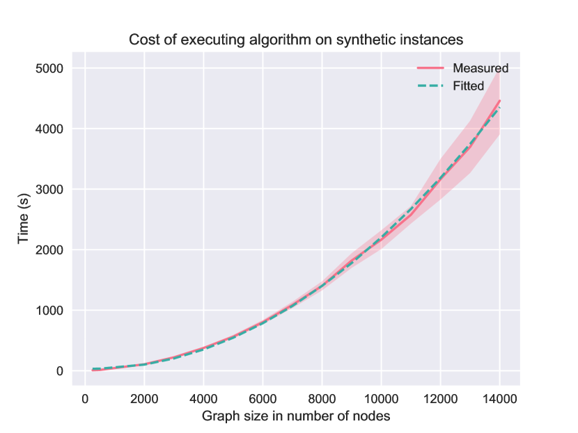
Figure 4: Performance of the proposed algorithm in synthetic datasets.

VII Conclusions

In this work, we presented Chimera a novel shared factorization overtime model that can simultaneously take the link, content, and temporal information of networks into account improving over the state-of-the-art approaches for community detection. Our approach model and solve in efficient time the problem of combining link, content and temporal analysis for community detection and prediction in network data. Our method extracts the latent semantic structure of the network in multidimensional form, but in a way that takes into account the temporal continuity of the embeddings. Such approach greatly simplifies temporal analysis of the underlying network by using the embedding as a surrogate. A consequence of this simplification is that it is also possible to use this temporal sequence of embeddings to predict future communities with good results. The experimental results illustrate the effectiveness of Chimera, since it outperforms the baseline methods. Our experiments also show that the prediction is efficient in using embeddings to predict near future communities, which opens a vast array of new possibilities for exploration.

VIII Acknowlegments

Charu C. Aggarwal’s research was sponsored by the Army Research Laboratory and was accomplished under Cooperative Agreement Number W911NF-09-2-0053. The views and conclusions contained in this document are those of the authors and should not be interpreted as representing the official policies, either expressed or implied, of the Army Research Laboratory or the U.S. Government. The U.S. Government is authorized to reproduce and distribute reprints for Government purposes notwithstanding any copyright notation here on.

References

- [1] Earl R. Barnes “An Algorithm for Partitioning the Nodes of a Graph” In SIAM Journal on Algebraic Discrete Methods 3.4, 1982, pp. 541–550 DOI: 10.1137/0603056
- [2] Marya Bazzi et al. “Community detection in temporal multilayer networks, with an application to correlation networks” In Multiscale Modeling & Simulation 14.1 SIAM, 2016, pp. 1–41
- [3] James Bergstra, Daniel Yamins and David Cox “Making a science of model search: Hyperparameter optimization in hundreds of dimensions for vision architectures” In International Conference on Machine Learning, 2013, pp. 115–123
- [4] Vincent D Blondel, Jean-Loup Guillaume, Renaud Lambiotte and Etienne Lefebvre “Fast unfolding of communities in large networks” In Journal of Statistical Mechanics: Theory and Experiment 2008.10, 2008, pp. P10008
- [5] B. Bringmann, M. Berlingerio, F. Bonchi and A. Gionis “Learning and Predicting the Evolution of Social Networks” In IEEE Intelligent Systems 25.4, 2010, pp. 26–35 DOI: 10.1109/MIS.2010.91
- [6] Deepayan Chakrabarti, Ravi Kumar and Andrew Tomkins “Evolutionary clustering” In Proceedings of the 12th ACM SIGKDD international conference on Knowledge discovery and data mining, 2006, pp. 554–560 ACM
- [7] Yudong Chen, Vikas Kawadia and Rahul Urgaonkar “Detecting overlapping temporal community structure in time-evolving networks” In arXiv preprint arXiv:1303.7226, 2013
- [8] David Cohn and Thomas Hofmann “The Missing Link: A Probabilistic Model of Document Content and Hypertext Connectivity” In Proceedings of the 13th International Conference on Neural Information Processing Systems, NIPS’00 Denver, CO: MIT Press, 2000, pp. 409–415 URL: http://dl.acm.org/citation.cfm?id=3008751.3008811
- [9] David Cohn and Thomas Hofmann “The missing link-a probabilistic model of document content and hypertext connectivity” In Advances in neural information processing systems MIT; 1998, 2001, pp. 430–436
- [10] Santo Fortunato “Community detection in graphs” In Physics reports 486.3 Elsevier, 2010, pp. 75–174
- [11] Michelle Girvan and Mark EJ Newman “Community structure in social and biological networks” In Proceedings of the national academy of sciences 99.12 National Acad Sciences, 2002, pp. 7821–7826
- [12] B. Gliwa et al. “Different approaches to community evolution prediction in blogosphere” In 2013 IEEE/ACM International Conference on Advances in Social Networks Analysis and Mining (ASONAM 2013), 2013, pp. 1291–1298 DOI: 10.1145/2492517.2500231
- [13] Sunil Kumar Gupta et al. “Nonnegative shared subspace learning and its application to social media retrieval” In Proceedings of the 16th ACM SIGKDD international conference on Knowledge discovery and data mining, 2010, pp. 1169–1178 ACM
- [14] Jialin He and Duanbing Chen “A fast algorithm for community detection in temporal network” In Physica A: Statistical Mechanics and its Applications 429, 2015, pp. 87 –94 DOI: http://dx.doi.org/10.1016/j.physa.2015.02.069
- [15] Jake M Hofman and Chris H Wiggins “Bayesian approach to network modularity” In Physical review letters 100.25 APS, 2008, pp. 258701
- [16] N. Ilhan and I. G. Ögüdücü “Community Event Prediction in Dynamic Social Networks” In 2013 12th International Conference on Machine Learning and Applications 1, 2013, pp. 191–196 DOI: 10.1109/ICMLA.2013.40
- [17] Nagehan İlhan and Şule Gündüz Öğüdücü “Feature identification for predicting community evolution in dynamic social networks” In Engineering Applications of Artificial Intelligence 55, 2016, pp. 202 –218 DOI: https://doi.org/10.1016/j.engappai.2016.06.003
- [18] Nagehan İlhan and Şule Gündüz Öğüdücü “Predicting Community Evolution Based on Time Series Modeling” In Proceedings of the 2015 IEEE/ACM International Conference on Advances in Social Networks Analysis and Mining 2015, ASONAM ’15 Paris, France: ACM, 2015, pp. 1509–1516 DOI: 10.1145/2808797.2808913
- [19] M. Jamali, G. Haffari and M. Ester “Modeling the Temporal Dynamics of Social Rating Networks Using Bidirectional Effects of Social Relations and Rating Patterns” In 2010 IEEE International Conference on Data Mining Workshops, 2010, pp. 344–351 DOI: 10.1109/ICDMW.2010.103
- [20] Vikas Kawadia and Sameet Sreenivasan “Sequential detection of temporal communities by estrangement confinement” In Scientific reports 2 Nature Publishing Group, 2012
- [21] Min-Soo Kim and Jiawei Han “A particle-and-density based evolutionary clustering method for dynamic networks” In Proceedings of the VLDB Endowment 2.1 VLDB Endowment, 2009, pp. 622–633
- [22] Jure Leskovec, Kevin J. Lang, Anirban Dasgupta and Michael W. Mahoney “Statistical Properties of Community Structure in Large Social and Information Networks” In Proceedings of the 17th International Conference on World Wide Web, WWW ’08 Beijing, China: ACM, 2008, pp. 695–704 DOI: 10.1145/1367497.1367591
- [23] Yu-Ru Lin et al. “Facetnet: a framework for analyzing communities and their evolutions in dynamic networks” In Proceedings of the 17th international conference on World Wide Web, 2008, pp. 685–694 ACM
- [24] Liyuan Liu, Linli Xu, Zhen Wangy and Enhong Chen “Community Detection Based on Structure and Content: A Content Propagation Perspective” In Data Mining (ICDM), 2015 IEEE International Conference on, 2015, pp. 271–280 IEEE
- [25] Christopher D. Manning, Prabhakar Raghavan and Hinrich Schütze “Introduction to Information Retrieval” New York, NY, USA: Cambridge University Press, 2008
- [26] Ramesh M. Nallapati, Amr Ahmed, Eric P. Xing and William W. Cohen “Joint Latent Topic Models for Text and Citations” In Proceedings of the 14th ACM SIGKDD International Conference on Knowledge Discovery and Data Mining, KDD ’08 Las Vegas, Nevada, USA: ACM, 2008, pp. 542–550 DOI: 10.1145/1401890.1401957
- [27] Ramesh M Nallapati, Amr Ahmed, Eric P Xing and William W Cohen “Joint latent topic models for text and citations” In Proceedings of the 14th ACM SIGKDD international conference on Knowledge discovery and data mining, 2008, pp. 542–550 ACM
- [28] B. Ngonmang and E. Viennet “Toward Community Dynamic through Interactions Prediction in Complex Networks” In 2013 International Conference on Signal-Image Technology Internet-Based Systems, 2013, pp. 462–469 DOI: 10.1109/SITIS.2013.81
- [29] M. E. G. Pavlopoulou, G. Tzortzis, D. Vogiatzis and G. Paliouras “Predicting the evolution of communities in social networks using structural and temporal features” In 2017 12th International Workshop on Semantic and Social Media Adaptation and Personalization (SMAP), 2017, pp. 40–45 DOI: 10.1109/SMAP.2017.8022665
- [30] Anna-Kaisa Pietilänen and Christophe Diot “Dissemination in Opportunistic Social Networks: The Role of Temporal Communities” In Proceedings of the Thirteenth ACM International Symposium on Mobile Ad Hoc Networking and Computing, MobiHoc ’12 Hilton Head, South Carolina, USA: ACM, 2012, pp. 165–174 DOI: 10.1145/2248371.2248396
- [31] Erzsébet Ravasz et al. “Hierarchical organization of modularity in metabolic networks” In science 297.5586 American Association for the Advancement of Science, 2002, pp. 1551–1555
- [32] Peter J Rousseeuw “Silhouettes: a graphical aid to the interpretation and validation of cluster analysis” In Journal of computational and applied mathematics 20 Elsevier, 1987, pp. 53–65
- [33] Yiye Ruan, David Fuhry and Srinivasan Parthasarathy “Efficient Community Detection in Large Networks Using Content and Links” In Proceedings of the 22Nd International Conference on World Wide Web, WWW ’13 Rio de Janeiro, Brazil: ACM, 2013, pp. 1089–1098 DOI: 10.1145/2488388.2488483
- [34] S. Saganowski “Predicting community evolution in social networks” In 2015 IEEE/ACM International Conference on Advances in Social Networks Analysis and Mining (ASONAM), 2015, pp. 924–925 DOI: 10.1145/2808797.2809353
- [35] Bobak Shahriari et al. “Taking the human out of the loop: A review of bayesian optimization” In Proceedings of the IEEE 104.1 IEEE, 2016, pp. 148–175
- [36] A. Sharma et al. “Predicting small group accretion in social networks: A topology based incremental approach” In 2015 IEEE/ACM International Conference on Advances in Social Networks Analysis and Mining (ASONAM), 2015, pp. 408–415 DOI: 10.1145/2808797.2808914
- [37] M. Takaffoli, R. Rabbany and O. R. Zaïane “Community evolution prediction in dynamic social networks” In 2014 IEEE/ACM International Conference on Advances in Social Networks Analysis and Mining (ASONAM 2014), 2014, pp. 9–16 DOI: 10.1109/ASONAM.2014.6921553
- [38] Xuning Tang and Christopher C Yang “Dynamic community detection with temporal dirichlet process” In Privacy, Security, Risk and Trust (PASSAT) and 2011 IEEE Third Inernational Conference on Social Computing (SocialCom), 2011 IEEE Third International Conference on, 2011, pp. 603–608 IEEE
- [39] Duncan J Watts, Peter Sheridan Dodds and Mark EJ Newman “Identity and search in social networks” In science 296.5571 American Association for the Advancement of Science, 2002, pp. 1302–1305
- [40] Han Xu, Eric Martin and Ashesh Mahidadia “Exploiting Paper Contents and Citation Links to Identify and Characterise Specialisations” In 2014 IEEE International Conference on Data Mining Workshop, 2014, pp. 613–620 IEEE
- [41] Tianbao Yang, Rong Jin, Yun Chi and Shenghuo Zhu “Combining Link and Content for Community Detection: A Discriminative Approach” In Proceedings of the 15th ACM SIGKDD International Conference on Knowledge Discovery and Data Mining, KDD ’09 Paris, France: ACM, 2009, pp. 927–936 DOI: 10.1145/1557019.1557120
- [42] Wenchao Yu, Charu C. Aggarwal and Wei Wang “Temporally Factorized Network Modeling for Evolutionary Network Analysis” In Proceedings of the Tenth ACM International Conference on Web Search and Data Mining, WSDM ’17 Cambridge, United Kingdom: ACM, 2017, pp. 455–464 DOI: 10.1145/3018661.3018669
- [43] Ding Zhou et al. “Probabilistic Models for Discovering e-Communities” In Proceedings of the 15th International Conference on World Wide Web, WWW ’06 Edinburgh, Scotland: ACM, 2006, pp. 173–182 DOI: 10.1145/1135777.1135807
- [44] Yang Zhou, Hong Cheng and Jeffrey Xu Yu “Graph clustering based on structural/attribute similarities” In Proceedings of the VLDB Endowment 2.1 VLDB Endowment, 2009, pp. 718–729