Probability of inflation in Loop Quantum Cosmology

Abstract

We discuss how initial conditions for cosmological evolution can be defined in Loop Quantum Cosmology with massive scalar field and how the presence of the bounce influences the probability of inflation in this theory, compared with General Relativity. The main finding of the paper is existence of an attractor in the contracting phase of the universe, which results in special probability distribution at the bounce, quite independent on the measure of initial conditions in the remote past, and hence very specific duration of inflationary stage with the number of e-foldings about $140$.

I introduction

The concept of inflation has been originally proposed guth1981inflationary ; linde1982anew ; albrecht1982cosmology ; linde1983chaotic as a solution for various cosmological fine tuning, essentially horizon, homogeneity and flatness problems. An attractive side of inflation is that it can naturally produce small density perturbations which permit formation of the observed large scale structure of the universe out of quantum fluctuations mukhanov1992theoryof2 . However, the question about initial conditions for inflation itself remains open. Since there is no observational information from the early universe, one has to consider all possible initial conditions and to draw conclusions about the probability of inflation. Qualitative analysis of cosmological solutions in the case of Friedmann-Lemaitre-Robertson-Walker (FLRW) metric and a massive scalar field $\phi$ performed in belinsky1985inflationary ; 1985PhLB..155..232B has indicated the presence of attractor-like trajectories associated with inflation, showing that inflationary phase in cosmological evolution is almost generic.

Often pursued idea, as introduced in gibbons1987anatural , is to define a Liouville’s measure on the phase space of the system, for instance for massive scalar field in the homogeneous universe, so called minisuperspace approximation. Despite existing criticism (see e.g schiffrin2012measure ), measure defined in this way is widely used, due to lack of information about initial conditions or physical preference for particular states of the universe. One of the objections has been the fact that the total measure diverges, as a result of unbounded volume variable hawking1988howprobable , that can be treated in different ways carroll2010unitary ; gibbons2008measure , possibly leading to different results, for a recent review see brandenberger2017initial . Attractor-like behavior found in belinsky1985inflationary seemed to contradict the Liouville’s theorem, which does not allow for attractor solutions remmen2013attractor . This issue has been clarified in ref. corichi2014inflationary , where the apparent attractor in the phase space $\left(\phi,\dot{\phi}\right)$, where $\dot{\phi}$ is time derivative of $\phi$, is associated with an exponential increase of the physical volume during inflation. There the measure is defined on a surface of constant Hubble rate $H$ and then, using Hamiltonian constraint, is reduced to the form

$$\varOmega=g\left(H,\phi\right)\mathrm{d}\phi\mathrm{d}v,$$ (1)

where $v$ is volume of the universe. Probability of some states is given by the ratio of the integrals of $\varOmega$ over a part of the phase space containing those states to the same integral taken over the whole phase space. Divergence in both integrals is avoided by imposing a cut-off in volume variable. Conclusion drawn from the analysis is that inflation is generically highly probable for various potentials and measures.

General relativity (GR) itself does not prescribe how to set up initial conditions, and it was proposed in belinsky1985inflationary that the boundary of applicability of classical solutions (defined from the equality of the energy density to Planck’s value) can be chosen as the place where initial conditions should be defined with equal probability in each point. The discussion on possible choices of the measure is given in 1987ZhETF..93..784B , where in particular choices made in belinsky1985inflationary and gibbons1987anatural are compared. The conserved measure $\mathcal{F}$ is defined by the vanishing divergence

$$\partial_{i}\left(\mathcal{F}v^{i}\right)=0,$$ (2)

where $v^{i}$ is Hamiltonian flow vector. The measure of the finite bundle is defined by the integral over the part of the hypersurface $\Delta S$ from which the bundle emanates

$$\mu=\int_{\Delta S}\mathcal{F}v^{i}ds_{i},$$ (3)

where $ds_{i}$ is the hypersurface element. The conservation of such a measure along the flow and the fact that it is independent of the choice of the initial hypersurface are ensured by Eq. (2). It is argued that each particular choice of the measure corresponds to a choice of a particular exact solution of Eq. (2) and there exists no indication on physical ground how this choice should be made. In other words, as such the choice of the measure is arbitrary and additional external arguments should be involved in order to specify it uniquely. In particular, the choice made in belinsky1985inflationary is based on the argument of inapplicability of classical dynamics beyond the quantum boundary.

Since the Liouville’e measure diverges for the flat $k=0$ cosmological models gibbons2008measure ; corichi2014inflationary , qualitatively different approach is introduced by Remmen and Carroll remmen2013attractor in context of massive scalar field in flat FLRW universe within GR. Instead of defining the measure on constant density surface they showed in which sense $\left(\phi,\dot{\phi}\right)$ space can be regarded as effective phase space. Considering the measure density $f$ in this effective phase space they demonstrated that such a measure exists for single scalar field cosmologies, and that apparent attractor behavior corresponds to the divergence of the measure $f$, which satisfies the same type of equation as Eq. (2) for the induced Hamiltonian flow vector $\mathbf{v}$.

Inflation, being very powerful idea in resolving several problems of the Big Bang cosmology, does not provide a solution for initial singularity problem borde2003inflationary , despite some set of nonsingular solutions within GR exists, e.g. page1984afractal . Loop quantum gravity thiemann2003lectures ; ashtekar2004background ; rovelli2004quantum is a nonperturbative background independent quantization of GR. Application of its techniques to homogeneous systems is called loop quantum cosmology (LQC) bojowald2008loopquantum . On the genuine quantum level as a sort of general regularity result one can consider a global boundedness of the matter energy density operator in LQC. In terms of trajectories the regularity and in particular the presence of the bounce has been established for several example models (varying in matter content and the topology of Cauchy slices), which include in particular the model of ashtekar2006quantum ; ashtekar2006quantum2 . More general results have been obtained on the level of the so called classical effective dynamics. In particular, for the model admitting a massive scalar field with quadratic potential the regularity has been shown in singh2006nonsingular . The closest to general statement in the context of isotropic LQC is the content of work 2009CQGra..26l5005S . Hence in LQC the quantum boundary is naturally replaced by a bounce on which the energy density of the universe reaches maximum. One may attempt to define the measure of inflationary solutions at the bounce. The first treatment of the measure problem in LQC along these lines is given in ashtekar2010loopquantum following the approach in corichi2014inflationary , but with different regularization of infinities. Allowing all possible initial conditions at the bounce and constructing dynamical trajectories numerically, it is found in ref. ashtekar2010loopquantum that the probability of inflation with more than 68 e-foldings (necessary to explain observations) is almost unity for massive scalar field in flat FLRW universe. Comparison of their result and explanation of the apparent contradiction with the corresponding one for GR, obtained in ref. gibbons2008measure , is given in ref. corichi2011measure . However, setting initial conditions at the bounce might look an artificial choice.

As the main feature of LQC cosmology with respect to GR is the presence of the bounce, the question about prebounce cosmological evolution, when the universe is contracting, arises. Generally speaking, one can expect that contracting universe is highly inhomogeneous and anisotropic 1989NYASA.571..249P . In absence of reliable description of such contracting phase, following linsefors2013duration ; bolliet_clarifications_2017 , we adopt the same cosmological equations of semiclassical LQC and study the possibility to set up initial conditions in the remote past of this cosmological model, namely in the contracting phase prior to the bounce, characterized by the oscillatory behavior of the scalar field, and analyze the consequences, in particular for the generality of inflation.

Our paper is organized as follows. In the next section we introduce the system and relevant equations, summarizing the effective dynamics in the LQC perspective. In Sec. III we discuss different choices of the measure on the set of initial conditions and explore three different choices of the initial probability distributions. We discuss and interpret obtained results in Sec. IV which also concludes the paper.

II Effective dynamics in LQC

In LQC the gravitational sector of the phase space is denoted by two conjugate variables, connection and the triad, which encode curvature and spatial geometry, respectively (see e.g. a review 2011CQGra..28u3001A ). In this work we consider only flat homogeneous and isotropic spacetime in which case the dynamical part of the connection is determined by a single quantity labeled $\mathfrak{c}$ and likewise the triad by a parameter $p$, related by the Poisson bracket $\left\{\mathfrak{c},p\right\}=8\pi G\gamma/3$, where $\gamma$ is the Immirzi parameter whose value $\gamma\thickapprox 0.2375$ is set by black hole entropy calculation thiemann2003lectures ; ashtekar2004background ; rovelli2004quantum ; ashtekar2006quantum ; domagala2004blackhole ; meissner2004blackhole . Relation with the usual GR scale factor $a$ is

$$\mathfrak{c}=\gamma\dot{a},\qquad p=a^{2}.$$ (4)

We set $c=1$ and use Planck units; Planck length $l_{\mathrm{{\scriptscriptstyle\textrm{P}l}}}=\sqrt{\hbar G}$ , mass $M_{\mathrm{{\scriptscriptstyle\textrm{P}l}}}=\sqrt{\hbar/G}$ and density $\rho_{\mathrm{{\scriptscriptstyle\textrm{P}l}}}=1/\hbar G^{2}$ .

While the gravitational variables $\mathfrak{c}$ and $p$ are directly related to the basic canonical pair in loop quantum gravity, the LQC equations are simpler in the coordinates

$$b=\frac{\mathfrak{c}}{\sqrt{|p|}}=\gamma H,\qquad\mathfrak{v}=\frac{|p|^{3/2}}{2\pi G\hbar\gamma}=\frac{a^{3}}{2\pi G\hbar\gamma},$$ (5)

related by the Poisson bracket $\left\{b,\mathfrak{v}\right\}=2/\hbar.$ $H=\dot{a}/a$ is the Hubble rate.

Up to a good approximation, the quantum dynamics of LQC can be described as an effective theory singh2005semiclassical ; taveras2008corrections ; banerjee2005discreteness generated by an effective Hamiltonian constraint

$$\mathcal{H}_{{\scriptscriptstyle\mathrm{eff}}}=-\frac{3\hbar}{4\gamma\lambda^{2}}\mathfrak{v}\sin^{2}\left(\lambda b\right)+\mathcal{H}_{{\scriptscriptstyle\mathrm{M}}},$$ (6)

here $\lambda^{2}=4\sqrt{3}\pi\gamma l_{\mathrm{{\scriptscriptstyle\textrm{P}l}}}^{2}$ is the ’area gap’, the lowest eigenvalue of the area operator in loop quantum gravity, and $\mathcal{H}_{{\scriptscriptstyle\mathrm{M}}}$ is the matter Hamiltonian. In our case of a massive scalar field $\phi$ with its canonical momentum $\Pi_{\phi}=\dot{\phi}a^{3}$ and potential $V\left(\phi\right),$ it is given by

$$\mathcal{H}_{{\scriptscriptstyle\mathrm{M}}}=\frac{1}{2}\frac{\Pi_{\phi}^{2}}{a^{3}}+a^{3}V\left(\phi\right)=a^{3}\rho.$$ (7)

Energy density and pressure of the scalar field are, as in the classical case, given by

$$\rho=\frac{1}{2}\dot{\phi}^{2}+V\left(\phi\right),\qquad p_{\phi}=\frac{1}{2}\dot{\phi}^{2}-V\left(\phi\right).$$ (8)

Using Hamilton’s equations for $\dot{\phi}$ and $\dot{\Pi}_{\phi}$ the equation for the scalar field is obtained

$$\ddot{\phi}+3H\dot{\phi}+V^{\prime}\left(\phi\right)=0,$$ (9)

where $V^{\prime}\left(\phi\right)=\partial V/\partial\phi$. Hamilton’s equation for $\mathfrak{v}$ is

$$\dot{\mathfrak{v}}=\left\{\mathfrak{v},\mathcal{H}_{{\scriptscriptstyle\mathrm{eff}}}\right\}=-\frac{2}{\hbar}\frac{\partial\mathcal{H}_{{\scriptscriptstyle\mathrm{eff}}}}{\partial b}=\frac{3}{\gamma\lambda}\mathfrak{v}\sin\left(\lambda b\right)\cos\left(\lambda b\right).$$ (10)

Using the definition for $\mathfrak{v}$ (5) we can rewrite $\dot{\mathfrak{v}}$ as

$$\dot{a}=\frac{a}{\gamma\lambda}\sin\left(\lambda b\right)\cos\left(\lambda b\right).$$ (11)

Now, combining (11) with the vanishing Hamiltonian constraint, $\mathcal{H}_{{\scriptscriptstyle\mathrm{eff}}}=0$, we get modified Friedmann equation singh2006nonsingular ; ashtekar2006quantum2

$$H^{2}=\frac{8\pi G}{3}\rho\left(1-\frac{\rho}{\rho_{c}}\right),$$ (12)

with the critical density

$$\rho_{c}=\frac{3}{8\pi G\gamma^{2}\lambda^{2}}=\frac{\sqrt{3}}{32\pi^{2}\gamma^{3}}\rho_{\mathrm{{\scriptscriptstyle\textrm{P}l}}}.$$ (13)

For $\gamma\thickapprox 0.2375$ we have $\rho_{c}\thickapprox 0.41\rho_{\mathrm{{\scriptscriptstyle\textrm{P}l}}},$ used in numerical calculation. We will consider scalar field with the mass $m$ and potential

$$V\left(\phi\right)=\frac{m^{2}}{2}\phi^{2}.$$ (14)

The main difference from the GR is realized as an additional term, quadratic in energy density of the scalar field, in Friedmann equation (12). It comes out that a quantum geometric effect is negligible for small density, and in the limit $\rho\ll\rho_{c}$ one recovers ordinary Friedmann equation. In fact, in this limit, where the analysis of belinsky1985inflationary is valid, $H$ can be expressed from (12) and substituted into (9) leaving only two independent variables: $\phi$ and $\dot{\phi}$. That is also possible to do in the bouncing cosmologies (with two independent $\phi-\dot{\phi}$ diagrams for both positive and negative values of $H$), see e.g. vereshchagin2003flatcosmological . However, a quantum geometric effect has a strong effect when density is comparable to the critical one, see Fig. 1. Both density and Hubble rate are bounded from above and, going back in time, instead of running into singularity with diverging physical variables, Hubble rate vanishes as density approaches the critical value and universe undergoes regular evolution through the bounce bojowald2001absence

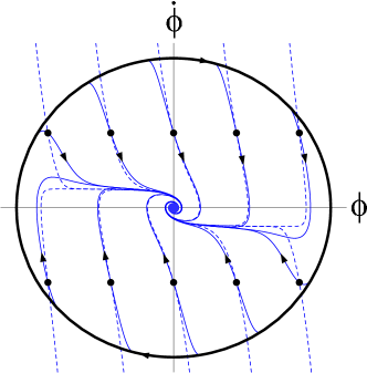
Figure 1: GR versus LQC inflationary solutions. Reproduced from Ref. singh2006nonsingular .

III Choices of the measure

As we pointed out in the introduction, LQC incorporates a regular evolution through the bounce and a description of the prebounce history. Thus, within LQC it is natural to set up initial conditions in the remote past linsefors2013duration , which in homogeneous and isotropic case corresponds to the contraction with oscillating scalar field. As there is no unique way to choose the measure on the initial surface, in what follows we consider three different choices of measure.

One may argue for the naturalness of the particular definition, as done in gibbons1987anatural for a measure obtained from the symplectic form of a phase space. This measure diverges for a flat universe, but the field variables completely specify the system, defining the effective two-dimensional phase space, and providing a way of finding on it the unique measure, conserved under the Hamiltonian flow vector. This is the approach developed in remmen2013attractor and is the base of our first choice of measure.

Another possibility is commonly assumed flat probability distribution. Particularly, we take the phase of the field on the initial surface as a natural random parameter, in accordance with the arguments in belinsky1985inflationary and assumed in linsefors2013duration with whom we compare our results. And, finally, the third distribution we consider is arbitrarily chosen step function in the angle variable.

III.1 Remmen and Carroll measure

In this subsection we introduce the notion of an effective phase space and probability measure defined on it, following Remmen and Carroll remmen2013attractor . The question they discuss is if $\left(\phi,\dot{\phi}\right)$ space could indeed be considered as an effective phase space and how, if at all, unique conserved measure can be defined on it. We present here the line of thought and main results, referring the reader to remmen2013attractor for the full derivation and accompanying discussion.

Being a $2n$-dimensional symplectic manifold, phase space $\Gamma$ has a closed two-form defined on it;

$$\omega=\sum_{i=1}^{n}\mathrm{d}p_{i}\wedge\mathrm{d}q^{i},$$ (15)

where $\left(q^{i},p_{i}\right)$ are canonical coordinates and their conjugate momenta. Liouville’s measure is then

$$\Omega=\frac{\left(-1\right)^{n(n-1)/2}}{n!}\omega^{n}.$$ (16)

Liouville’s theorem states that this measure is conserved along the Hamiltonian flow vector $X_{\mathcal{H}}$, that can be expressed by vanishing Lie derivative of $\Omega$, $\mathcal{L}_{X_{\mathcal{H}}}\Omega=0.$ In canonical formulation of GR Hamiltonian is seen as a constraint, i.e. trajectories are confined to a $\left(2n-1\right)$-dimensional hypersurface $C$ in $\Gamma,$

$$C=\Gamma/\left\{\mathcal{H}=const.\right\}.$$ (17)

Evolution of trajectories in $C$ is described by Hamiltonian flow vector $X_{\mathcal{H}}$ given by

$$X_{\mathcal{H}}=\frac{\partial\mathcal{H}}{\partial p_{i}}\frac{\partial}{\partial q^{i}}-\frac{\partial\mathcal{H}}{\partial q^{i}}\frac{\partial}{\partial p_{i}}.$$ (18)

Space of trajectories then can be defined as $M=C/X_{\mathcal{H}}.$ Unique (under some reasonable conditions) measure on $M$ for FLRW universe is obtained from the symplectic form $\omega$ by identifying the $n$th phase space coordinate as time $t$ gibbons1987anatural , $\omega=\tilde{\omega}+\mathrm{d}\mathcal{H}\wedge\mathrm{d}t.$ The corresponding measure is

$$\Theta=\frac{\left(-1\right)^{\left(n-1\right)(n-2)/2}}{\left(n-1\right)!}\tilde{\omega}^{n-1}.$$ (19)

We can think of $\left(\phi,\dot{\phi}\right)$ space as an effective phase space if it captures the entire dynamics of the system. Eliminating $a$ and $\dot{a}$ from the dynamics, possible only in flat FLRW model, and expressing $H$ as a function of $\phi$ and $\dot{\phi}$ by use of Friedmann equation, reduces Hamiltonian flow vector (18) to only two components, $\phi$ and $\dot{\phi}$. It means that if we consider the map $\chi:C\rightarrow K\cong\left(\phi,\dot{\phi}\right)$ defined by

$$\chi\left(a,\dot{a},\phi,\dot{\phi}\right)=\left(\phi,\dot{\phi}\right)$$ (20)

it represents a vector field invariant with respect to the Hamiltonian flow vector $X_{\mathcal{H}}$. Roughly speaking, we have unique (no intersecting trajectories) induced Hamiltonian vector field on $\left(\phi,\dot{\phi}\right)$, reflecting the behavior of the Hamiltonian vector field of the full phase space. All points in $3-$dimensional constrained surface $C$ with the same $\left(\phi,\dot{\phi},\,\textrm{sign}(H)\right)$ values are mapped into one point in $\left(\phi,\dot{\phi}\right)$ space. In GR the effective phase space is the entire $\phi-\dot{\phi}$ plane. In LQC the phase space is composed of two ellipsoidal sheets, one for each $\textrm{sign}(H)$, glued together at their boundaries, corresponding to $H=0$. On both sheets the phase space trajectories do not intersect. So the effective dynamics of LQC can be considered as a Hamiltonian flow on the reduced phase space of nontrivial topology.

We denote induced vector field as $\mathbf{v}$ and define $x=\phi,\,y=\dot{\phi}$. The measure on $\left(\phi,\dot{\phi}\right)$ is a two-form $\boldsymbol{\mathbf{\sigma}}$ that can be written as

$$\boldsymbol{\mathbf{\sigma}}=f\left(x,y\right)\mathrm{d}x\wedge\mathrm{d}y$$ (21)

for some function $f$. Conservation of the measure along $\mathbf{v}$ is provided by $\mathcal{L}_{\mathbf{v}}\boldsymbol{\mathbf{\sigma}}=0,$ which can be expressed as

$$\nabla\left(f\mathbf{v}\right)=0.$$ (22)

It was shown 1987ZhETF..93..784B ; remmen2013attractor that if there exist a function $f$ satisfying (22), it defines the measure on effective phase space uniquely, i.e.

$$\mathrm{d}\Pi_{\phi}\wedge\mathrm{d}\phi=f\mathrm{d}\dot{\phi}\wedge\mathrm{d}\phi,$$ (23)

where $\Pi_{\phi}$ is momentum conjugate to $\phi$ in $\left(\phi,\dot{\phi}\right)$ space. Equation (23) shows that the natural Liouville measure is equivalent to the measure $f\mathrm{d}\dot{\phi}\wedge\mathrm{d}\phi$ introduced by Remmen and Carroll remmen2013attractor .

The vector field $\mathbf{v}$ is given by

$$\mathbf{v}=\dot{\phi}\boldsymbol{\mathbf{\hat{\phi}}}+\ddot{\phi}\boldsymbol{\hat{\dot{\phi}}},$$ (24)

where $\ddot{\phi}$ is obtained from (9) and $H$ from (12). If we define the coordinates

$$x=\phi=\frac{r}{m}\cos\theta,\qquad y=\dot{\phi}=r\sin\theta,$$ (25)

we have

$$\rho=\frac{r^{2}}{2},\qquad H^{2}=\frac{4\pi Gr^{2}}{3}\left(1-\frac{r^{2}}{2\rho_{c}}\right),$$ (26)

and vector field $\mathbf{v}$ in polar coordinates:

$$\mathbf{v}=-3rH\sin^{2}\theta\mathbf{\hat{r}}-r\left(m+3H\sin\theta\cos\theta\right)\boldsymbol{\hat{\theta}},$$ (27)

where we have used standard transformation

$$\mathbf{\hat{x}}=m\cos\theta\mathbf{\hat{r}}-m\sin\theta\boldsymbol{\hat{\theta}},\quad\;\mathbf{\hat{y}}=\sin\theta\mathbf{\hat{r}}+\cos\theta\boldsymbol{\hat{\theta}}.$$ (28)

Constraint (22) on the measure density $f\left(r,\theta\right)$ then becomes partial differential equation

$$\frac{1}{r}\partial_{r}\left(Hr^{2}f\right)\sin^{2}\theta+\frac{m}{3}\partial_{\theta}f+H\partial_{\theta}\left(f\sin\theta\cos\theta\right)=0.$$ (29)

Inserting eq. (26) into eq. (29) one can derive the following result (the corresponding result within the general relativity is obtained in remmen2013attractor ),

$$f=A\left[\frac{1}{r^{3}\sqrt{1-\frac{r^{2}}{2\rho_{c}}}}+\frac{2\sqrt{3\pi G}\sin\theta\cos\theta}{mr^{2}}\right],\;A\epsilon\mathbb{R},$$ (30)

with the plus sign coming from the negative $H.$

A measure on the space of trajectories (as opposed to the effective phase space) can be constructed from the effective phase space measure on any surface transverse to those trajectories, by demanding that the physical result be independent of the chosen transverse curve remmen2014howmany . It can be any transverse slicing that evolves monotonically in time, so we will take $r\,\left(\propto\sqrt{\rho}\right)=const$ surface and parametrize it by the angular coordinate $\theta$. For a bundle of trajectories centered at the angle $\theta_{1}$ and spanned by $\textrm{d}\theta_{1}$ on initial surface at the radius $r,$ we can write its probability measure as $P\left(\theta_{1}\right)\textrm{d}\theta_{1}$ and let it evolve to another surface $r=r_{2}.$ Condition for the measure to be conserved is then

$$P\left(\theta_{1}\right)|_{r_{1}}\textrm{d}\theta_{1}=P\left(\theta_{2}\right)|_{r_{2}}\textrm{d}\theta_{2}.$$ (31)

Now, for a region $\textrm{d}\theta_{1}\textrm{d}r_{1}$ that evolves to $\textrm{d}\theta_{2}\textrm{d}r_{2}$, we have Liouville’s theorem for the effective phase space

$$f\left(r_{1},\theta_{1}\right)\textrm{d}\theta_{1}\textrm{d}r_{1}=f\left(r_{2},\theta_{2}\right)\textrm{d}\theta_{2}\textrm{d}r_{2},$$ (32)

i.e. $f$ satisfies (22). Comparing (31) and (32) we conclude that the probability distribution on the space of trajectories, $r=const$ surface, is $P\left(\theta\right)|_{r}\propto f\textrm{$\left(r,\theta\right)$d}r$. We could have first divide (32) by $\textrm{d}t$ (which we can do since $t$ evolves uniformly for all trajectories) thus obtaining

$$P\left(\theta\right)|_{r}\propto f\left(r,\theta\right)|\dot{r}|,$$ (33)

with the proportionality constant given by the normalization $\intop_{0}^{2\pi}P\left(\theta\right)|_{r}\textrm{d}\theta$=1. For (30) and

$$|\dot{r}|=\left|-\frac{3H}{r}\dot{\phi}^{2}\right|\simeq 2\sqrt{3\pi G}r^{2}\sin^{2}\theta$$ (34)

we finally obtain

$$P\left(\theta\right)|_{r}=\frac{\sin^{2}\theta}{\pi}+\sqrt{\frac{3G}{\pi}}\frac{2r\,\sin^{3}\theta\cos\theta}{m}.$$ (35)

This probability distribution of initial conditions is used below to infer the generality of inflation.

III.2 Linsefors and Barrau measure

Closely following Linsefors and Barrau linsefors2013duration , we define again $x=\phi,\,y=\dot{\phi}$ so that $\rho=\frac{1}{2}\left(m^{2}x^{2}+y^{2}\right)$ and equations of motion for $x,$$y$ and $\rho$ are

$$\dot{x}=y,\qquad\dot{y}=-3Hy-m^{2}x,\qquad\dot{\rho}=-3Hy^{2}.$$ (36)

Given the conditions for the prebounce oscillations,

$$\rho\ll\rho_{c},\qquad|H|\ll m;\qquad H\approx-\sqrt{\frac{8\pi G\rho}{3}},$$ (37)

we can approximate $x$ and $y$ by

$$x=\frac{\sqrt{\rho}}{m}\sin\left(mt+\delta\right),\qquad y=\sqrt{\rho}\cos\left(mt+\delta\right),$$ (38)

which gives

$$\dot{\rho}=\sqrt{24\pi G}\rho^{3/2}\cos^{2}\left(mt+\delta\right)$$ (39)

with the solution

$$\rho=\rho_{0}\left[1-\sqrt{\frac{3\pi G\rho_{0}}{2}}\left(t+\frac{1}{2m}\sin\left(2mt+2\delta\right)\right.\right.$$

$$\left.\left.-\frac{1}{2m}\sin\left(2\delta\right)\right)\right]^{-2}.$$ (40)

Note the presence of an additional term with respect to the corresponding Eq. $\left(8\right)$ in linsefors2013duration . In Fig. 2 we present phase space trajectories on the $\phi-\dot{\phi}$ plane near the origin, where Eq. (40) is valid. In the limit $t\rightarrow-\infty$ one keeps just the term proportional to $t^{-2}$ in (40) (see e.g. belinsky1985inflationary ) corresponding to the solutions shown in Fig. 2a, where the blue circle represents the constant density surface. Full expression for the density, on the other hand gives rise to a more complex structure shown in Fig. 2b.

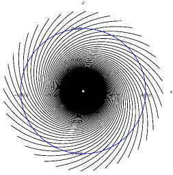
(a) Only the term $t^{-2}$ is kept. Blue circle shows the boundary $\rho_{0}$ where initial conditions are set.

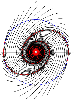
(b) Full asymptotic solution of the same equations corresponding to Eq. (40). Red curves denote repulsive separatrices.

Figure 2: Asymptotic solution of cosmological equations of LQC with massive scalar field in the limit $\rho\rightarrow 0$ corresponding to Eqs. (38) and (40). The origin is denoted by white circle.

The assumption on the measure in linsefors2013duration is that the probability of initial conditions does not depend on $\delta$, namely

$$P(\delta)=const.$$ (41)

For comparison with the previous subsection, notice $\delta=\pi/2-\theta|_{t=0}$.

Comparing Fig. 2 a) and b) one can understand the emergence of the separatrix at the contraction phase. This separatrix is repulsive, in contrast to the attractive inflationary separatrix at the expansion phase. It breaks down the symmetry of solution shown in Fig. 2a and introduce an additional dependence of the probability of solutions on the phase $\delta$ and on the mass $m$, see Eq. (40).

After the oscillatory phase ends most solutions do not follow this separatrix and this gives origin to the tendency of the trajectories to end up with high probability at the same point at the bounce. Although this has been observed in linsefors2013duration , the explanation was lacking.

III.3 Narrow distribution

As a third choice of the measure we adopt for the probability distribution two short intervals of widths equal to $\pi/20$, with constant probability within. This choice of the measure is not motivated by any physical arguments, it just represents a narrow distribution in angle variable and we intend to compare the probability distribution at the bounce with other choices of the measure discussed above.

III.4 Results

The set of initial probability density distributions is shown in Fig. 4a. For the probability distribution (41) we examine the dependence of the value of the field at the bounce on the mass, by choosing initial conditions at some $r_{0}\ll m$, evolving them up to the bounce and computing the mean $\left\langle...\right\rangle$ and the standard deviation $\sigma_{B}$ of the quantity $\phi_{B}\,\textrm{sign}\left(\dot{\phi}_{B}\right)$. Solutions at the bounce can be parametrized by $\phi_{B}$ and $\textrm{sign}\left(\dot{\phi}_{B}\right)$ but, as done in linsefors2013duration we project them to the physically relevant parameters. Repeating the calculation for different masses while keeping the ratio $r_{0}/m=0.005$, we obtain the result shown in Fig. 3, which can be reasonably fit with the formulas

$$\left\langle m\phi_{B}\,\textrm{sign}\left(\dot{\phi}_{B}\right)\right\rangle = m\left(0.32+0.16\,Log\left(\frac{1}{m}\right)\right),\>\;$$ (42)

$$\sigma_{B} = 0.16m.$$ (43)

These results imply that for $m\ll M_{\mathrm{{\scriptscriptstyle\textrm{P}l}}}$ for most trajectories the bounce occurs with $\sigma_{B}$ and $\phi_{B}\ll M_{\mathrm{{\scriptscriptstyle\textrm{P}l}}}$.

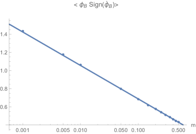
(a) Dependence of the peak of probability density distribution on scalar field mass.

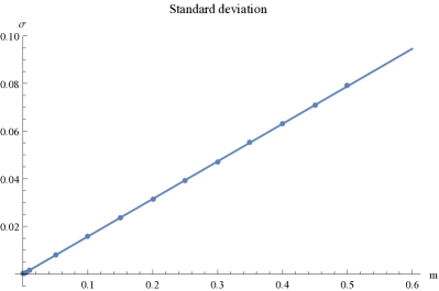
(b) Dependence of the standard deviation in the probability density distribution on scalar field mass.

Figure 3: Mass is given in Planck units.

We repeat the process of evolving trajectories and computing the mean of the field value at the bounce for all three choices of measure with the fixed mass $m=1.21\cdot 10^{-6}M_{\mathrm{{\scriptscriptstyle\textrm{P}l}}}$, chosen for comparison with linsefors2013duration . The obtained probability density distributions of the variable $\left\langle m\,\phi_{B}\,\textrm{sign}\left(\dot{\phi}_{B}\right)\right\rangle$ at the bounce are shown in Fig. 4b. For initial conditions with the probability (41) we find good agreement with the result of linsefors2013duration where the distribution is found to be sharply peaked around $3.55\cdot 10^{-6}M_{\mathrm{{\scriptscriptstyle\textrm{P}l}}}^{2}.$

Surprisingly, other very different probability distributions also result in a similar distributions at the bounce, despite so different choices of the measure in the remote past. The field variable $\left\langle\phi_{B}\,\textrm{sign}\left(\dot{\phi}_{B}\right)\right\rangle$ is narrowly distributed in the region $\dot{\phi}\ll M_{\mathrm{{\scriptscriptstyle\textrm{P}l}}}^{2}$ at the bounce for all cases considered. Thus, our results show that there exists a kind of attractor also in the contracting branch, and the field values on the bounce are virtually independent of the initial probability distribution, as long at it is smooth.

The number of e-folds during slow-roll inflation can be estimated following linsefors2013duration as

$$N=2\pi\textup{G}\phi_{max}^{2},$$ (44)

so knowing the maximum value of the scalar field reached after the bounce we can estimate the value of $N$. Since $\phi_{max}\approx 2\phi_{B}$ we find $N\approx 170$.

We calculate numerically the number of e-foldings corresponding to the mean field value at the bounce for the three cases, using

$$N=\int_{t_{in}}^{t_{end}}H\mathrm{d}t,$$ (45)

where $t_{in}$ and $t_{end}$ are the initial and ending time of the inflation, respectively. As the start of the inflation we take the time when field takes the maximum value after the bounce, and for the end we take the $|H|=m$ condition. Particularly, we do not include super-inflation phase into the number of e-folds calculation. We get $N\approx 143$ for the first two, and $N\approx 153$ for the third initial distribution.

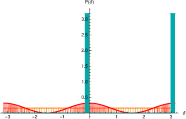
(a) Probability distributions for initial conditions in the remote past given by: Eq. (41) - orange, Eq. (35) - red, narrow distribution - blue. Vertical lines denote the values of $\delta$ variable used in the calculations.

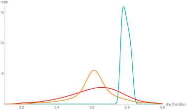
(b) Probability distribution of the rescaled field values at the bounce.

Figure 4: Initial probability distributions and probability distributions at the bounce for all three cases considered.

Therefore, it is the main result of this paper that the probability distribution at the bounce strongly depends on mass of the scalar field, but weakly depends on initial probability distribution in the remote past.

IV Discussion and conclusions

The main question arising from the results reported above is why most solutions originating from the oscillatory contracting phase end up at the bounce having very restricted values of the scalar field? This can be understood as a consequence of the presence of repulsive separatrix at the contraction phase, as well as small value of the mass of the scalar field, compared with the Planck mass, see Fig. 5.

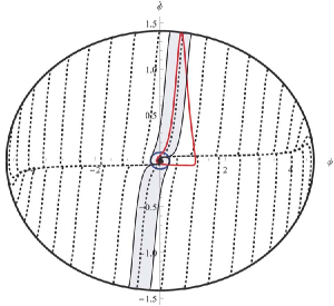
Figure 5: Solutions of the cosmological equations of LQC in the $\phi-\dot{\phi}$ diagram. All solutions start in the distant past in the origin, pass through oscillatory phase with increasing amplitude of oscillations and end up at the bounce shown by the thick external circle. Blue internal circle (obtained setting $H=m$) represents the region where most solutions deviate from the repulsive separatrix (located along the horizontal axis, at which the Hubble parameter is nearly constant). This region shrinks with decreasing mass (the value of the mass in this figure is $m=0.1M_{\mathrm{{\scriptscriptstyle\textrm{P}l}}}$ selected for better clarity). The red curve shows the complete most probable solution originating from the remote past (including both contraction and expansion phases). This solution has no exponential contraction phase, but it has a successful inflationary phase.

Due to repulsive nature of the separatrix, most solutions, starting at the origin, do not follow along it, and deviate from it as early as possible. The separatrix appears at small enough densities, see Fig. 2b above. However, all solutions are located between the pair of repulsive separatrices as long as the solution is oscillating near the origin $\rho=0$. This behavior breaks down when $H\sim m$, see Fig. 5. Then most solutions cannot propagate to large values of $\phi$ at the contraction phase and leave the region near the origin in the vertical direction (see shaded region in Fig. 5). This picture corresponds exactly to Fig. 4b.

Therefore, indeed as pointed out in linsefors2013duration , there is a preferred set of cosmological solutions in LQC, which have no exponential contraction phase, but possess a successful inflationary phase. This is a direct consequence of the prebounce evolution in LQC, specifically existence of the repulsive separatrix in contracting phase. In other words, one may say that there is an attractor behavior in LQC, which not only ensures the successful inflation, but also determines the prebounce evolution in LQC. This attractor is shown in Fig. 5 by the red curve.

Contrary to the assumptions made in previous literature,e.g. in ashtekar2010loopquantum ; corichi2011measure ; corichi2014inflationary , one consequence of our analysis is a well defined probability distribution for the scalar field at the bounce. This probability distribution is strongly peaked at some particular scalar field values, see Fig. 4b. This result hence impacts on the prediction of the duration of inflation, and it can be subject to precision tests, such as CMB anisotropy measurements.

The analysis of this paper was based on the simplest quadratic effective potential for the scalar field. Clearly, many inflationary potentials share qualitative features with such quadratic potential, see e.g. singh2006nonsingular , therefore we expect that obtained results are generic for inflationary scenarios in Loop Quantum Cosmology.

Acknowledgments: we thank both referees for their remarks, which allowed to improve presentation of our results.

References

- (1) A. H. Guth, Physical Review D 23, 347 (1981).
- (2) A. Linde, Physics Letters B 108, 389 (1982).
- (3) A. Albrecht and P. J. Steinhardt, Physical Review Letters 48, 1220 (1982).
- (4) A. Linde, Physics Letters B 129, 177 (1983).
- (5) V. F. Mukhanov, H. A. Feldman, and R. H. Brandenberger, Physics Reports 215, 203 (1992).
- (6) V. A. Belinskii, L. P. Grishchuk, I. M. Khalatnikov, and Y. B. Zeldovich, Sov. Phys. JETP 62, 195 (1985).
- (7) V. A. Belinsky, L. P. Grishchuk, I. M. Khalatnikov, and Y. B. Zeldovich, Physics Letters B 155, 232 (1985).
- (8) G. Gibbons, S. Hawking, and J. Stewart, Nuclear Physics B 281, 736 (1987).
- (9) J. S. Schiffrin and R. M. Wald, Physical Review D 86 (2012).
- (10) S. Hawking and D. N. Page, Nuclear Physics B 298, 789 (1988).
- (11) S. M. Carroll and H. Tam, arXiv:1007.1417 [astro-ph, physics:gr-qc, physics:hep-th] (2010), arXiv: 1007.1417.
- (12) G. W. Gibbons and N. Turok, Physical Review D 77 (2008).
- (13) R. Brandenberger, International Journal of Modern Physics D 26, 1740002 (2017).
- (14) G. N. Remmen and S. M. Carroll, Physical Review D 88 (2013).
- (15) A. Corichi and D. Sloan, Classical and Quantum Gravity 31, 062001 (2014).
- (16) V. A. Belinskii and I. M. Khalatnikov, Sov. Phys. JETP 66, 441 (1987).
- (17) A. Borde, A. H. Guth, and A. Vilenkin, Physical Review Letters 90 (2003).
- (18) D. N. Page, Classical and Quantum Gravity 1, 417 (1984).
- (19) T. Thiemann, Lectures on Loop Quantum Gravity, in Quantum Gravity, edited by R. Beig et al., volume 631, pages 41–135, Springer Berlin Heidelberg, Berlin, Heidelberg, 2003.
- (20) A. Ashtekar and J. Lewandowski, Classical and Quantum Gravity 21, R53 (2004).
- (21) C. Rovelli, Quantum Gravity, Cambridge University Press, Cambridge, 2004.
- (22) M. Bojowald, Living Reviews in Relativity 11 (2008).
- (23) A. Ashtekar, T. Pawlowski, and P. Singh, Physical Review D 74 (2006).
- (24) A. Ashtekar, T. Pawlowski, and P. Singh, Physical Review D 73 (2006).
- (25) P. Singh, K. Vandersloot, and G. V. Vereshchagin, Physical Review D 74 (2006).
- (26) P. Singh, Classical and Quantum Gravity 26, 125005 (2009).
- (27) A. Ashtekar and D. Sloan, Physics Letters B 694, 108 (2010).
- (28) A. Corichi and A. Karami, Physical Review D 83 (2011).
- (29) R. Penrose, Annals of the New York Academy of Sciences 571, 249 (1989).
- (30) L. Linsefors and A. Barrau, Phys. Rev. D87, 123509 (2013).
- (31) B. Bolliet, A. Barrau, K. Martineau, and F. Moulin, Classical and Quantum Gravity 34, 145003 (2017).
- (32) A. Ashtekar and P. Singh, Classical and Quantum Gravity 28, 213001 (2011).
- (33) M. Domagala and J. Lewandowski, Class. Quantum Grav. 21, 5233 (2004).
- (34) K. A. Meissner, Classical and Quantum Gravity 21, 5245 (2004).
- (35) P. Singh and K. Vandersloot, Physical Review D 72 (2005).
- (36) V. Taveras, Physical Review D 78 (2008).
- (37) K. Banerjee and G. Date, Class. Quantum Grav. 22, 2017 (2005).
- (38) G. V. Vereshchagin, International Journal of Modern Physics D 12, 1487 (2003).
- (39) M. Bojowald, Physical Review Letters 86, 5227 (2001).
- (40) G. N. Remmen and S. M. Carroll, Phys. Rev. D90, 063517 (2014).